Chapter 3. Lebesgue integral and the monotone convergence ...richardt/MA2224/MA2224-ch3.pdf ·...

Chapter 3. Lebesgue integral and the monotone convergencetheoremContents

3.1 Starting point — a σ-algebra and a measure . . . . . . . . . . . . . . . . . . . . 13.2 Measurable functions . . . . . . . . . . . . . . . . . . . . . . . . . . . . . . . . 33.3 Limits of measurable functions . . . . . . . . . . . . . . . . . . . . . . . . . . . 83.4 Simple functions . . . . . . . . . . . . . . . . . . . . . . . . . . . . . . . . . . 93.5 Positive measurable functions . . . . . . . . . . . . . . . . . . . . . . . . . . . 133.6 Integrable functions . . . . . . . . . . . . . . . . . . . . . . . . . . . . . . . . . 173.7 Functions integrable on subsets . . . . . . . . . . . . . . . . . . . . . . . . . . . 19

3.1 Starting point — a σ-algebra and a measureRemark 3.1.1. What we need to define integrals of R-valued functions, apart from a considerableamount of the terminology we have come across so far, is that

• we have R and the Borel σ-algebra on it; this will come in for the values of the functionswe consider;

• on the domain we need a measure, and a measure needs a σ-algebra. We will use (R,L , µ),where L is the σ-algebra of Lebesgue measurable sets and µ : L → [0,∞] is the measuregiven by µ(F ) = m∗(F ) for F ∈ L .

In fact, we could equally well have a more general domain X and we would need a σ-algebraΣ of subsets of X together with a measure µ : Σ → [0,∞]. That is we could treat

∫Xf dµ =∫

Xf(x) dµ(x), integrals of (certain) functions f : X → R with general domains X , provided we

have (X,Σ, µ), but we will mostly stick to f : R→ R where (X,Σ, µ) = (R,L , µ = m∗|L ).One advantage of sticking to domain X = R is that we can picture our functions as graphs

y = f(x) in R2. We could still have that advantage if we allowed X ⊆ R, for instance to define∫[a,b]

f dµ where f : [a, b] → R. Actually this case will be included rather easily, but anotherperspective is to generalise to multiple integrals, that is to integrals of functions f : Rn → R. Weare not ready for that because we only did m∗ as length outer measure on R. For R2, we wouldneed to do something similar to what we did with length to define area measure. The startingpoint would be areas of rectangles, and we would need to replace what we did with the intervalalgebra J by stuff about a ‘rectangle algebra’. Some of the details at the start would be a bitdifferent but many of the same proofs can be used in R2, and for volume outer measure in R3

and more generally for n-dimensional measure in Rn.However, what we do in this chapter can be done in considerable generality and we set out

the general definitions concisely.

Definition 3.1.2. If X is a set then a collection Σ ⊆ P(X) is called a σ-algebra (of subsets ofX) if it satisfies:

2 2017–18 Mathematics MA2224

(i) ∅ ∈ Σ

(ii) E ∈ Σ⇒ Ec ∈ Σ

(iii) E1, E2, . . . ∈ Σ⇒⋃∞n=1En ∈ Σ.

A pair (X,Σ) of a setX and a σ-algebra of subsets ofX is sometimes called a measurable space.

Definition 3.1.3. If Σ is a σ-algebra (of subsets of set X) and µ : Σ→ [0,∞] is a function, thenwe call µ a measure on Σ if it satisfies

(a) µ(∅) = 0

(b) µ is countably additive, that is whenever E1, E2, . . . ∈ Σ are disjoint, then µ (⋃∞n=1En) =∑∞

n=1 µ(En).

The combination (X,Σ, µ) is called a measure space and the subsets E ⊂ X with E ∈ Σ arecalled measurable subsets (with respect to the given Σ). If in addition µ(X) = 1, then µ is calleda probability measure and the combination (X,Σ, µ) is called a probability space. In the contextof probability, measurable subsets E ∈ Σ are called events and µ(E) ∈ [0, 1] the probability ofthe event E.

Examples 3.1.4.

1. Our primary focus will be (X,Σ, µ) = (R,L , µ) with µ = m∗|L being Lebesgue lengthmeasure on the σ-algebra L of Lebesgue measurable subsets of R.

2. If X ∈ L then we can define a σ-algebra Σ on X and a measure λ : Σ→ R by

Σ = {F ∩X : F ∈ L }

andλ(F ∩X) = µ(F ∩X) = m∗(F ∩X).

It may be helpful to have a notation LX for this Σ (though that is not a standard notation).

Proof. There is nothing difficult in this except perhaps that there is a possibility of confu-sion between two notions of complement. Perhaps this can be solved if we write R \E forthe complement of E ⊆ R and X \E for the complement of E ⊆ X as a subset of X . Thenotation we usually use of Ec for the complement of E is not very adaptable to more thanone meaning of complement.

Notice that, since X ∈ L , we could also say

Σ = {E ∈ L : E ⊆ X}

(because E ∈ L with E ⊆ X implies E = E ∩X , and on the other hand F ∈ L impliesthat E = F ∩X ∈ L and has E ⊆ X). So ∅ ∈ Σ, E ∈ Σ⇒ X \E = X ∩ (R \E) ∈ Σ.Moreover E1, E2, . . . ∈ Σ implies

⋃∞n=1En ∈ Σ.

The properties required for λ to be a measure are just true because we know µ is a measure.

Lebesgue integral 3

3. If X = [0, 1], then the previous example turns into an example of a probability space([0, 1],Σ, λ).

4. If (X,Σ, µ1) and (X,Σ, µ2) are two measure spaces with the same underlying set andσ-algebra, and if c1, c2 ≥ 0, then we can get a new measure µ = c1µ1 + c2µ2 on Σ bydefining

µ(E) = c1µ1(E) + c2µ2(E) (E ∈ Σ)

(This is easy to check and we can leave it as an exercise.)

3.2 Measurable functionsDefinition 3.2.1. A function f : R → R is called Lebesgue measurable (or measurable withrespect to the measurable space (R,L )) if for each a ∈ R

{x ∈ R : f(x) ≤ a} = f−1((−∞, a]) ∈ L .

Examples 3.2.2. (i) Continuous functions f : R→ R are always measurable, because (−∞, a]is a closed subset and so f−1((−∞, a]) is closed, hence in L .

If you prefer to think about open sets, (a,∞) is open, so f−1((a,∞)) is open, hence in L ,hence its (closed) complement (f−1((a,∞)))c = f−1((a,∞)c) = f−1((−∞, a]) is in L .

(ii) The characteristic function χQ of the rationals is measurable (but not continuous anywhere).

The reason is that the set Q ∈ L (it is a countable union of single point sets, hence aBorel set, hence in L ; another way is to use m∗(Q) = 0 to get Q ∈ L ) and so then is itscomplement R \Q ∈ L . For f = χQ, we can see that

f−1((−∞, a]) = {x ∈ R : f(x) ≤ a} =

∅ if a < 0

R \Q if 0 ≤ a < 1

R if a ≥ 1

and in all cases we get a set in L .

(iii) For a subset E ⊆ R, its characteristic function χE is a measurable function if and only ifE ∈ L (which means E is a measurable set). As in the previous case, for f = χE , we cansee that

f−1((−∞, a]) = {x ∈ R : f(x) ≤ a} =

∅ if a < 0

R \ E if 0 ≤ a < 1

R if a ≥ 1

Certainly ∅,R ∈ L and we have R \ E ∈ L ⇐⇒ E ∈ L .

Remark 3.2.3. Our aim will be to define integrals for all measurable functions, but we will notquite succeed in that.


Proposition 3.2.4. If f : R→ R is Lebesgue measurable, then

f−1(B) ∈ L

for each Borel set B.

Proof. LetΣf = {E ⊆ R : f−1(E) ∈ L }.

We claim that Σf is a σ-algebra.That is quite easy to verify.

(i) f−1(∅) = ∅ ∈ L ⇒ ∅ ∈ Σf

(ii) E ∈ Σf ⇒ f−1(E) ∈ L ⇒ f−1(Ec) = (f−1(E))c ∈ L ⇒ Ec ∈ Σf

(iii) E1, E2, . . . ∈ Σf ⇒ f−1(En) ∈ L for n = 1, 2, . . .. From this we have⋃∞n=1 f

−1(En) ∈L and so

f−1

(∞⋃n=1

En

)=∞⋃n=1

f−1(En) ∈ L ⇒∞⋃n=1

En ∈ Σf

As we know f is Lebesgue measurable, we have

(−∞, a] ∈ Σf (∀a ∈ R)

and that means that Σf contains the σ-algebra generated by {(−∞, a] : a ∈ R} — which weknow to be the Borel σ-algebra by Corollary 2.3.13.

Proposition 3.2.5. If f, g : R → R are Lebesgue measurable functions and c ∈ R, then thefollowing are also Lebesgue measurable functions

cf, f 2, f + g, fg, |f |,max(f, g)

The idea here is to combine functions by manipulating their values at a point. So fg : R→ Ris the function with value at x ∈ R given by (fg)(x) = f(x)g(x), and similarly for the otherfunctions.

Proof. cf : First if c = 0, cf is the zero function, which is measurable (very easy to check thatdirectly). Let h = cf (so that h(x) = cf(x)). For c > 0, then

h−1((−∞, a]) = {x ∈ R : cf(x) ≤ a} = {x ∈ R : f(x) ≤ a/c} ∈ L

and so h = cf is Lebesgue measurable. For c < 0,

h−1((−∞, a]) = {x ∈ R : f(x) ≥ a/c} = f−1([a/c,∞)) ∈ L

using Proposition 3.2.4 and the fact that [a/c,∞) is a Borel set.

Lebesgue integral 5

f 2: Here we say

{x ∈ R : f(x)2 ≤ a} =

{∅ if a < 0

f−1([−√a,√a]) if a ≥ 0

f + g: (This is perhaps the most tricky part.) Fix a ∈ R and we aim to show that {x ∈ R :f(x) + g(x) ≤ a} ∈ L . Taking the complement, this would follow from {x ∈ R :f(x) + g(x) > a} ∈ L .

For any x where f(x) + g(x) > a then f(x) > a − g(x) and there is a rational q ∈ Q sothat f(x) > q > a− g(x). Then g(x) > a− q. So

x ∈ Sq = f−1((q,∞)) ∩ g−1((a− q,∞))

for some q ∈ Q. On the other hand if f(x) > q and g(x) > a− q, then f(x) + g(x) > a,from which we conclude that

{x ∈ R : f(x) + g(x) > a} =⋃q∈Q

Sq.

By Proposition 3.2.4 Sq ∈ L for each q and hence {x ∈ R : f(x) + g(x) > a} ∈ L(because it is countable union of sets Sq ∈ L ).

fg: This follows from the previous parts because fg = ((f + g)2 − (f − g)2)/4.

|f |: This is easy as {x ∈ R : |f(x)| ≤ a} = ∅ if a < 0 but is f−1([−a, a]) if a ≥ 0.

max(f, g): {x ∈ R : max(f(x), g(x)) ≤ a} = f−1((−∞, a]) ∩ g−1((−∞, a]).

Remark 3.2.6. It is convenient to allow for functions that sometimes have the value ∞ andsometimes −∞. For that we need to introduce the extended real line [−∞,∞], which is Rwith two extra elements −∞ and +∞ added. This is similar to our earlier use of [0,∞].

We order [−∞,∞] so that −∞ < x < ∞ for each x ∈ R. We introduce arithmetic on[−∞,∞] in a similar way to what we did before for [0,∞] but we do not allow subtraction of∞from itself or −∞ from itself. We extend the usual arithmetic operations on R with the rules

x+∞ =∞+ x = ∞x+ (−∞) = (−∞) + x = (−∞) (for x ∈ R)

x∞ =∞x = ∞ = (−∞)(−x) = (−x)(−∞)

x(−∞) = (−∞)x = (−∞) = (−x)(∞) = (∞)(−x) (for 0 < x ∈ R)

0∞ =∞0 = 0

0(−∞) = (−∞)0 = 0

From the point of view of the ordering of [−∞,∞], there is a strictly monotone increasingbijection φ : R→ (−1, 1) given by

φ(x) =x

1 + |x|


and both φ and φ−1 are continuous (so that φ is a homeomorphism). We can extend φ to get anorder-preserving bijection Φ: [−∞,∞] → [−1, 1] by defining Φ(−∞) = −1, Φ(x) = φ(x) forx ∈ R and Φ(∞) = 1. Since we know that nonempty subsets of [−1, 1] have both a supremumand an infimum, it follows by applying Φ−1 that all nonempty subsets of [−∞,∞] also have asupremum (least upper bound) and infimum (greatest lower bound).

We define convergence on [−∞,∞] such that Φ becomes a homeomorphism onto [−1, 1](which means for example that limn→∞ xn = ` has the standard meaning if all the terms xn andthe limit ` are finite, but limn→∞ xn = ∞ means limn→∞Φ(xn) = Φ(∞) = 1 or that given anyM < ∞, there is N so that M < xn ≤ ∞ holds for all n > N ). It is also true that monotoneincreasing sequences (xn)∞n=1 in [−∞,∞] always converge (to supn xn in fact) and so also domonotone decreasing sequences always converge (to their infimum).

Definition 3.2.7. A function f : R → [−∞,∞] is called Lebesgue measurable (or measurablewith respect to the measurable space (R,L )) if for each a ∈ R

{x ∈ R : −∞ ≤ f(x) ≤ a} = f−1([−∞, a]) ∈ L .

Note that this definition agrees with the earlier Definition 3.2.1 if f(x) ∈ R always (becausethen f−1([−∞, a]) = f−1((−∞, a])).

Proposition 3.2.8. Let f : R → [−∞,∞] be a function and let A = {x ∈ R : f(x) = −∞} =f−1({−∞}), B = {x ∈ R : f(x) =∞} = f−1({∞}). Then the following are equivalent

(a) f is Lebesgue measurable

(b) A,B ∈ L and the function g : R→ R given by

g(x) =

{f(x) if −∞ < x <∞0 if x ∈ A ∪B

is Lebesgue measurable.

Proof. (a)⇒ (b): Note that

A =∞⋂n=1

f−1([−∞,−n]) ∈ L

(because σ-algebras are closed under the operation of taking countable intersections) and

R \B =∞⋃n=1

f−1([−∞, n]) ∈ L ⇒ B ∈ L

(countable unions and complements stay in L ).To show that g is measurable, note that

g−1((−∞, a]) =

{f−1([−∞, a]) ∪B if a ≥ 0

f−1([−∞, a]) \ A if a < 0

Lebesgue integral 7

So g−1((−∞, a]) ∈ L for each a.(b)⇒ (a): Note that

f−1([−∞, a]) =

{g−1((−∞, a]) \B if a ≥ 0

g−1((−∞, a]) ∪ A if a < 0

and so f−1([−∞, a]) ∈ L for each a (using (b)).

Remark 3.2.9. We can also define measurability of functions defined on Lebesgue measurablesubsets X ⊂ R, as follows. This would include for example the situation where X is an intervalof any kind, or any Borel set (which includes open subsets X of R, in particular).

Definition 3.2.10. If X ∈ L , then a function f : X → [−∞,∞] is called Lebesgue measurableon X if for each a ∈ R

{x ∈ X : −∞ ≤ f(x) ≤ a} = f−1([−∞, a]) ∈ L .

Proposition 3.2.11. Let X ∈ L and f : X → [−∞,∞]. Then the following are equivalent

(a) f is Lebesgue measurable on X

(b) the function g : R→ [−∞,∞] given by

g(x) =

{f(x) if x ∈ X0 if x ∈ R \X

is Lebesgue measurable on R.

Proof. For a ∈ R we have

g−1([−∞, a]) = {x ∈ R : −∞ ≤ g(x) ≤ a}

=

{(R \X) ∪ {x ∈ X : −∞ ≤ f(x) ≤ a} if a ≥ 0

{x ∈ X : −∞ ≤ f(x) ≤ a} if a < 0

So (a)⇒ (b). For the converse use

f−1([−∞, a]) =

{{x ∈ R : −∞ ≤ g(x) ≤ a} \ (R \X) if a ≥ 0

{x ∈ R : −∞ ≤ g(x) ≤ a} if a < 0

We can extend Proposition 3.2.5 to functions with values in [−∞,∞] except for one diffi-culty.

Proposition 3.2.12. If X ∈ L , c ∈ R and f, g : X → [−∞,∞] are Lebesgue measurablefunctions on X , then the following are also Lebesgue measurable functions (on X)

cf, f 2, fg, |f |,max(f, g)

If {x : f(x) =∞}∩{x : g(x) = −∞} = ∅ = {x : f(x) = −∞}∩{x : g(x) =∞}, then f + gis measurable (on X).

The proof (which we leave as an exercise) is to use Propositions 3.2.11, 3.2.8, and 3.2.5 forcf (c 6= 0), f 2, f + g, fg and |f |. For max(f, g) a similar proof can be used.


3.3 Limits of measurable functions

The next result shows that taking (pointwise) limits of sequence of measurable functions stillgive a measurable limit.

Definition 3.3.1. If fn : R → [−∞,∞] (n = 1, 2, . . .) is an infinite sequence of functions, thenwe say that f : R→ [−∞,∞] is the pointwise limit of the sequence (fn)n if we have

f(x) = limn→∞

fn(x)

for each x ∈ R.For any sequence fn : R→ [−∞,∞] we can define lim supn→∞ fn as the function with value

at x given by

lim supn→∞

fn(x) = limn→∞

(supk≥n

fk(x)

)(something that always makes sense because supk≥n fk(x) decreases as n increases — or at leastdoes not get any bigger as n increases).

Proposition 3.3.2. Let fn : R → [−∞,∞] (n = 1, 2, . . .) be Lebesgue measurable functions.Then

(a) the function x 7→ supn≥1 fn(x) is Lebesgue measurable;

(b) the function x 7→ infn≥1 fn(x) is Lebesgue measurable;

(c) lim supn→∞ fn is Lebesgue measurable; and

(d) if the pointwise limit function f : R→ [−∞,∞] exists, then f is Lebesgue measurable.

Proof. (a) If g(x) = supn≥1 fn(x), then g−1([−∞, a]) =⋂∞n=1 f

−1n ([−∞, a]) ∈ L (since the

σ-algebra L is closed under taking countable intersections).

(b) If g(x) = infn≥1 fn(x), then −g(x) = supn≥1(−fn(x)) is measurable by (a) and so then isg(x) measurable.

(c) We have lim supn→∞ fn(x) = infn≥1 gn(x) where gn(x) = supk≥n fk(x) is a decreasingsequence. But each gn is measurable by (b) and then lim supn→∞ fn(x) is measurable by(a).

(d) If the pointwise limit f(x) exists, then f(x) = lim supn→∞ fn(x), which is measurable by(c).

Lebesgue integral 9

3.4 Simple functionsDefinition 3.4.1. A function f : R → R is called a simple function if the range f(R) is a finiteset.

Note that we require finite values.

Proposition 3.4.2. Each simple function f : R→ R has a representation

f =n∑i=1

aiχEi

as a linear combination of finitely many characteristic functions of disjoint sets E1, E2, . . . , Enwith coefficients a1, a2, . . . , an ∈ R.

Moreover we can assume a1, a2, . . . , an are distinct values, that the Ej are all nonempty andthat

⋃nj=1Ej = R. With these assumptions the representation is called the standard representa-

tion and is unique apart from the order of the sum.A simple function is Lebesgue measurable if and only if the sets Ej in the standard represen-

tation are all in L .

Proof. Since f(R) is a finite set (and can’t be empty) we can list the elements f(R) = {y1, y2, . . . , yn}with n ≥ 1. Take Ej = f−1({yj}) = {x ∈ R : f(x) = yj} and then we get the standard repre-sentation f =

∑ni=1 yiχEi .

If f is measurable then Ej ∈ L for each j (because one point sets {aj} are Borel sets andwe can use Proposition 3.2.4).

Conversely, if each Ej is in L , then each χEj measurable, and then so is f measurable byProposition 3.2.5.

Notation 3.4.3. We will develop integration first for nonnegative measurable functions f : R →[0,∞].

To reduce the case of general (Lebesgue measurable) f : R → [−∞,∞] to the positive casewe will use the two associated functions f+ : R→ [0,∞] and f− : R→ [0,∞] given by

f+ = max(f, 0) =1

2(|f |+ f), f− = max(−f, 0) =

1

2(|f | − f),

both of which we know to be measurable. Notice that f = f+ − f− and |f | = f+ + f−.We call f+ the positive part of f and f− the negative part (but note that f− is positive also).

Definition 3.4.4. If f : R → [0,∞) is a nonnegative measurable simple function, with standardrepresentation f =

∑nj=1 ajχEj , then we define∫

Rf dµ =

n∑j=1

ajµ(Ej)

(where µ(Ej) means the Lebesgue measure ofEj). (Note that the integral makes sense in [0,∞].)


For E ∈ L , we define ∫E

f dµ =

∫RχEf dµ

(noting that χEf is also a nonnegative measurable simple function).

Examples 3.4.5. (i) For f = χ[0,1]+2χ[4,∞) the possible values are 0, 1 and 2, and the standardrepresentation is

f = χ[0,1] + 2χ[4,∞) + 0χ(−∞,0)∪(1,4)

so that∫Rf dµ = 1µ([0, 1]) + 2µ([4,∞)) + 0µ((−∞, 0) ∪ (1, 4)) = 1 +∞+ 0 =∞

(ii) For f = χQ, the standard representation is f = χQ + 0χR\Q and∫Rf dµ = 1µ(Q) + 0µ(R \Q) = 0 + 0 = 0

(iii) (Exercise) Show that if E ∈ L , then∫R χE dµ = µ(E).

Proposition 3.4.6. If f, g : R → [0,∞) are measurable simple functions and α ∈ [0,∞), thenαf , f + g are measurable simple functions and∫

Rαf dµ = α

∫Rf dµ,

∫R(f + g) dµ =

∫Rf dµ+

∫Rg dµ.

Proof. We know from Proposition 3.2.5 that αf , f + g are measurable.If α = 0, then 0f has standard representation 0 = 0χR and integral

∫R αf dµ =

∫R 0χR dµ =

0µ(R) = 0 = 0∫R f dµ = α

∫R f dµ. If α > 0 and f(R) = {a1, a2, . . . , an} let Fj = f−1({aj})

so that f has standard representation f =∑n

j=1 ajχFj , while αf has standard representationαf =

∑nj=1 αajχFj . So∫

Rαf dµ =

n∑j=1

(αaj)µ(Fj) = α

n∑j=1

ajµ(Fj) = α

∫Rf dµ.

To cope with h = f+g, let f(R) = {a1, a2, . . . , an}, Fj = f−1({aj}), g(R) = {b1, b2, . . . , bm},Gk = g−1({bk}). The range of h = f + g is certainly finite because it is contained in {aj + bk :1 ≤ j ≤ n, 1 ≤ k ≤ m}. So h is a simple function. Write h(R) = {c1, c2, . . . , cp} and then foreach 1 ≤ ` ≤ p we have

H` = h−1(c`) =⋃

{(j,k):aj+bk=c`}

Fj ∩Gk.

The sets making up H` are a disjoint union and so note that finite additivity of µ gives us

µ(H`) =∑

{(j,k):aj+bk=c`}

µ(Fj ∩Gk)

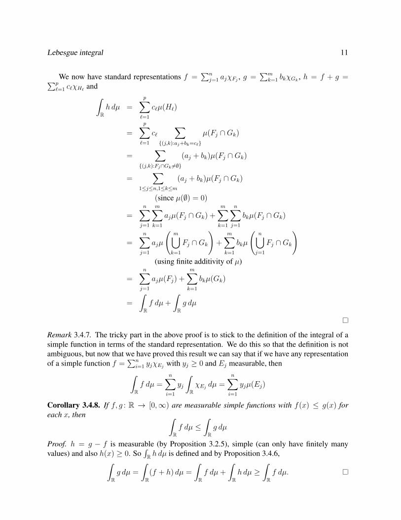
Lebesgue integral 11

We now have standard representations f =∑n

j=1 ajχFj , g =∑m

k=1 bkχGk , h = f + g =∑p`=1 c`χH` and∫

Rh dµ =

p∑`=1

c`µ(H`)

=

p∑`=1

c`∑

{(j,k):aj+bk=c`}

µ(Fj ∩Gk)

=∑

{(j,k):Fj∩Gk 6=∅}

(aj + bk)µ(Fj ∩Gk)

=∑

1≤j≤n,1≤k≤m

(aj + bk)µ(Fj ∩Gk)

(since µ(∅) = 0)

=n∑j=1

m∑k=1

ajµ(Fj ∩Gk) +m∑k=1

n∑j=1

bkµ(Fj ∩Gk)

=n∑j=1

ajµ

(m⋃k=1

Fj ∩Gk

)+

m∑k=1

bkµ

(n⋃j=1

Fj ∩Gk

)(using finite additivity of µ)

=n∑j=1

ajµ(Fj) +m∑k=1

bkµ(Gk)

=

∫Rf dµ+

∫Rg dµ

Remark 3.4.7. The tricky part in the above proof is to stick to the definition of the integral of asimple function in terms of the standard representation. We do this so that the definition is notambiguous, but now that we have proved this result we can say that if we have any representationof a simple function f =

∑ni=1 yjχEj with yj ≥ 0 and Ej measurable, then∫Rf dµ =

n∑i=1

yj

∫RχEj dµ =

n∑i=1

yjµ(Ej)

Corollary 3.4.8. If f, g : R → [0,∞) are measurable simple functions with f(x) ≤ g(x) foreach x, then ∫

Rf dµ ≤

∫Rg dµ

Proof. h = g − f is measurable (by Proposition 3.2.5), simple (can only have finitely manyvalues) and also h(x) ≥ 0. So

∫R h dµ is defined and by Proposition 3.4.6,∫

Rg dµ =

∫R(f + h) dµ =

∫Rf dµ+

∫Rh dµ ≥

∫Rf dµ.


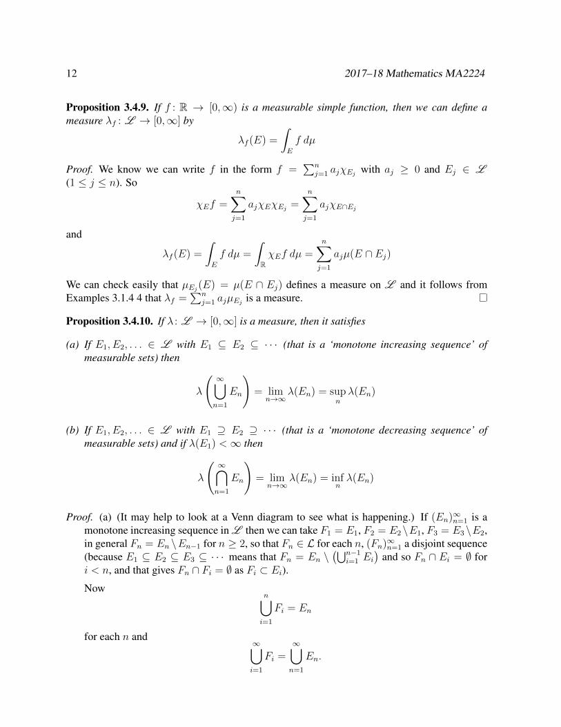
Proposition 3.4.9. If f : R → [0,∞) is a measurable simple function, then we can define ameasure λf : L → [0,∞] by

λf (E) =

∫E

f dµ

Proof. We know we can write f in the form f =∑n

j=1 ajχEj with aj ≥ 0 and Ej ∈ L(1 ≤ j ≤ n). So

χEf =n∑j=1

ajχEχEj =n∑j=1

ajχE∩Ej

and

λf (E) =

∫E

f dµ =

∫RχEf dµ =

n∑j=1

ajµ(E ∩ Ej)

We can check easily that µEj(E) = µ(E ∩ Ej) defines a measure on L and it follows fromExamples 3.1.4 4 that λf =

∑nj=1 ajµEj is a measure.

Proposition 3.4.10. If λ : L → [0,∞] is a measure, then it satisfies

(a) If E1, E2, . . . ∈ L with E1 ⊆ E2 ⊆ · · · (that is a ‘monotone increasing sequence’ ofmeasurable sets) then

λ

(∞⋃n=1

En

)= lim

n→∞λ(En) = sup

nλ(En)

(b) If E1, E2, . . . ∈ L with E1 ⊇ E2 ⊇ · · · (that is a ‘monotone decreasing sequence’ ofmeasurable sets) and if λ(E1) <∞ then

λ

(∞⋂n=1

En

)= lim

n→∞λ(En) = inf

nλ(En)

Proof. (a) (It may help to look at a Venn diagram to see what is happening.) If (En)∞n=1 is amonotone increasing sequence in L then we can take F1 = E1, F2 = E2\E1, F3 = E3\E2,in general Fn = En \En−1 for n ≥ 2, so that Fn ∈ L for each n, (Fn)∞n=1 a disjoint sequence(because E1 ⊆ E2 ⊆ E3 ⊆ · · · means that Fn = En \

(⋃n−1i=1 Ei

)and so Fn ∩ Ei = ∅ for

i < n, and that gives Fn ∩ Fi = ∅ as Fi ⊂ Ei).

Nown⋃i=1

Fi = En

for each n and∞⋃i=1

Fi =∞⋃n=1

En.


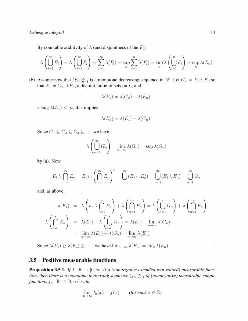
By countable additivity of λ (and disjointness of the Fi),

λ

(∞⋃i=1

Ei

)= λ

(∞⋃i=1

Fi

)=∞∑i=1

λ(Fi) = supn

n∑i=1

λ(Fi) = supnλ

(n⋃i=1

Fi

)= sup

nλ(En)

(b) Assume now that (En)∞n=1 is a monotone decreasing sequence in L . Let Gn = E1 \ En sothat E1 = Gn ∪ En, a disjoint union of sets on L, and

λ(E1) = λ(Gn) + λ(En).

Using λ(E1) <∞, this implies

λ(En) = λ(E1)− λ(Gn).

Since G1 ⊆ G2 ⊆ G3 ⊆ · · · we have

λ

(∞⋃n=1

Gn

)= lim

n→∞λ(Gn) = sup

nλ(Gn)

by (a). Now,

E1 \∞⋂n=1

En = E1 ∩

(∞⋂n=1

En

)c

=∞⋃n=1

(E1 ∩ Ecn) =

∞⋃n=1

(E1 \ En) =∞⋃n=1

Gn

and, as above,

λ(E1) = λ

(E1 \

∞⋂n=1

En

)+ λ

(∞⋂n=1

En

)= λ

(∞⋃n=1

Gn

)+ λ

(∞⋂n=1

En

)

λ

(∞⋂n=1

En

)= λ(E1)− λ

(∞⋃n=1

Gn

)= λ(E1)− lim

n→∞λ(Gn)

= limn→∞

λ(E1)− λ(Gn) = limn→∞

λ(En)

Since λ(E1) ≥ λ(E2) ≥ · · · , we have limn→∞ λ(En) = infn λ(En).

3.5 Positive measurable functionsProposition 3.5.1. If f : R → [0,∞] is a (nonnegative extended real valued) measurable func-tion, then there is a monotone increasing sequence (fn)∞n=1 of (nonnegative) measurable simplefunctions fn : R→ [0,∞) with

limn→∞

fn(x) = f(x) (for each x ∈ R)


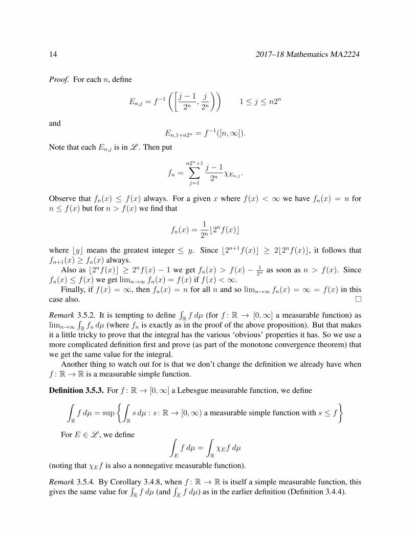
Proof. For each n, define

En,j = f−1([

j − 1

2n,j

2n

))1 ≤ j ≤ n2n

andEn,1+n2n = f−1([n,∞]).

Note that each En,j is in L . Then put

fn =n2n+1∑j=1

j − 1

2nχEn,j .

Observe that fn(x) ≤ f(x) always. For a given x where f(x) < ∞ we have fn(x) = n forn ≤ f(x) but for n > f(x) we find that

fn(x) =1

2nb2nf(x)c

where byc means the greatest integer ≤ y. Since b2n+1f(x)c ≥ 2b2nf(x)c, it follows thatfn+1(x) ≥ fn(x) always.

Also as b2nf(x)c ≥ 2nf(x) − 1 we get fn(x) > f(x) − 12n

as soon as n > f(x). Sincefn(x) ≤ f(x) we get limn→∞ fn(x) = f(x) if f(x) <∞.

Finally, if f(x) = ∞, then fn(x) = n for all n and so limn→∞ fn(x) = ∞ = f(x) in thiscase also.

Remark 3.5.2. It is tempting to define∫R f dµ (for f : R → [0,∞] a measurable function) as

limn→∞∫R fn dµ (where fn is exactly as in the proof of the above proposition). But that makes

it a little tricky to prove that the integral has the various ‘obvious’ properties it has. So we use amore complicated definition first and prove (as part of the monotone convergence theorem) thatwe get the same value for the integral.

Another thing to watch out for is that we don’t change the definition we already have whenf : R→ R is a measurable simple function.

Definition 3.5.3. For f : R→ [0,∞] a Lebesgue measurable function, we define∫Rf dµ = sup

{∫Rs dµ : s : R→ [0,∞) a measurable simple function with s ≤ f

}For E ∈ L , we define ∫

E

f dµ =

∫RχEf dµ

(noting that χEf is also a nonnegative measurable function).

Remark 3.5.4. By Corollary 3.4.8, when f : R → R is itself a simple measurable function, thisgives the same value for

∫R f dµ (and

∫Ef dµ) as in the earlier definition (Definition 3.4.4).


Lemma 3.5.5. For f, g : R→ [0,∞] Lebesgue measurable functions, we have

(a) if f ≤ g (pointwise) then ∫Rf dµ ≤

∫Rg dµ

(b) if E ⊂ F with E,F ∈ L , then ∫E

f dµ ≤∫F

f dµ

Proof. (a) if f ≤ g, then any simple function s : R→ [0,∞) with s ≤ f also has s ≤ g and so∫R s dµ ≤

∫R g dµ. Taking the supremum over all such s we get the result.

(b) Since E ⊂ F , we have χEf ≤ χFf and so∫E

f dµ =

∫RχEf dµ ≤

∫RχFf dµ =

∫F

f dµ

by (a).

Theorem 3.5.6 (Monotone Convergence Theorem). If fn : R→ [0,∞] is a monotone increasingsequence of (Lebesgue) measurable functions with pointwise limit f , then∫

Rf dµ = lim

n→∞

∫Rfn dµ

Proof. Notice that f(x) = limn→∞ fn(x) ∈ [0,∞] is guaranteed to exist as the sequence(fn(x))∞n=1 is monotone increasing. Moreover f is measurable (Proposition 3.3.2 (d)) and so∫R f dµ is defined by Definition 3.5.3.

From fn ≤ fn+1 we have fj(x) ≤ limn→∞ fn(x) = f(x) for each j. Hence∫R fj dµ ≤∫

R f dµ for each j by Lemma 3.5.5. Also∫R fn dµ ≤

∫R fn+1 dµ and so the sequence of integrals∫

R fn dµ is monotone increasing. That means limn→∞∫R fn dµ makes sense in [0,∞]. We have

limn→∞

∫Rfn dµ = sup

n≥1

∫Rfn dµ ≤

∫Rf dµ.

It remains to prove the reverse inequality.Fix a simple function s : R→ R with s(x) ≤ f(x) for all x ∈ R. We will show limn→∞

∫R fn dµ ≥∫

R s dµ and that will be enough because of the way∫R f dµ is defined.

To show this, fix α ∈ (0, 1) and consider

En,α = {x ∈ R : fn(x) ≥ αs(x)}

Notice that ∫En,α

αs dµ ≤∫En,α

fn dµ ≤∫Rfn dµ (1)


Because fn+1 ≥ fn we know En,α ⊂ En+1,α. For s(x) = 0, x ∈ En,α and for s(x) >0, limn→∞ fn(x) = f(x) ≥ s(x) > αs(x) implies x ∈ En,α when n is large enough. So⋃∞n=1En,α = R and Proposition 3.4.10 (with Proposition 3.4.9) tells us that∫

Rαs dµ = λαs(R) = λαs

(∞⋃n=1

En,α

)= lim

n→∞λαs(En,α) ≤ lim

n→∞

∫Rfn dµ

(using (1) at the last step). That gives us

α

∫Rs dµ =

∫Rαs dµ ≤ lim

n→∞

∫Rfn dµ.

As that is true for each α ∈ (0, 1), it follows that∫R s dµ ≤ limn→∞

∫R fn dµ, and so∫

Rf dµ = sup

{∫Rs dµ : s simple measureable, s ≤ f

}≤ lim

n→∞

∫Rfn dµ,

completing the proof.

Corollary 3.5.7. If f, g : R→ [0,∞] are (Lebesgue) measurable functions and α ≥ 0 then

(a)∫R αf dµ = α

∫R f dµ

(b)∫R(f + g) dµ =

∫R f dµ+

∫R g dµ

Proof. (a) By Proposition 3.5.1, there is a monotone increasing sequence (fn)∞n=1 of measurablesimple functions that converges pointwise to f . By the Monotone Convergence Theorem(3.5.6) we know that

∫R f dµ = limn→∞

∫R fn dµ. But also (αfn)∞n=1 is a sequence of mea-

surable simple functions that converges pointwise to αf and so we also have∫R αf dµ =

limn→∞∫R αfn dµ. Now from Proposition 3.4.6 we have

α

∫Rf dµ = lim

n→∞α

∫Rfn dµ = lim

n→∞

∫Rαfn dµ =

∫Rαf dµ

(b) Again by Proposition 3.5.1, there are monotone increasing sequences (fn)∞n=1 and (gn)∞n=1

of measurable simple functions with limn→∞ fn(x) = f(x) and limn→∞ gn(x) = g(x) foreach x ∈ R. By the Monotone Convergence Theorem (3.5.6) we know that

∫R f dµ =

limn→∞∫R fn dµ and

∫R g dµ = limn→∞

∫R gn dµ. But also (fn + gn)∞n=1 is a monotone

increasing sequence of measurable simple functions that converges pointwise to f + g andso we also have

∫R(f + g) dµ = limn→∞

∫R(fn + gn) dµ. From Proposition 3.4.6 we have∫

R(f + g) dµ = lim

n→∞

∫R(fn + gn) dµ

= limn→∞

(∫Rfn dµ+

∫Rgn dµ

)=

∫Rf dµ+

∫Rg dµ


Corollary 3.5.8. If f, g : R→ [0,∞] are (Lebesgue) measurable functions, α ≥ 0 and E ∈ L ,then ∫

E

(αf + g) dµ = α

∫E

f dµ+

∫E

g dµ

Proof. Apply Corollary 3.5.7 to χE(αf + g) = αχEf + χEg to get∫E

(αf + g) dµ =

∫RχE(αf + g) dµ

=

∫R(αχEf + χEg) dµ

= α

∫RχEf dµ+

∫RχEg dµ

= α

∫E

f dµ+

∫E

g dµ

3.6 Integrable functionsDefinition 3.6.1. If f : R → [−∞,∞] is measurable, then we say that f is Lebesgue integrableif ∫

Rf+ dµ <∞ and

∫Rf− dµ <∞.

For integrable f , we define ∫Rf dµ =

∫Rf+ dµ−

∫Rf− dµ

Lemma 3.6.2. If f : R→ [−∞,∞] is measurable, then f is Lebesgue integrable if and only if∫R|f | dµ <∞

Proof. If f is Lebesgue integrable, then |f | = f+ + f− is (Lebesgue) measurable and∫R|f | dµ =

∫Rf+ dµ+

∫Rf− dµ <∞.

Conversely, if f is Lebesgue integrable and∫R |f | dµ <∞, then f+ ≤ |f | (and we know f+

is measurable) and so ∫Rf+ dµ ≤

∫R|f | dµ <∞.

Similarly∫R f− dµ <∞.

Exercise 3.6.3. If f : R→ [−∞,∞] is (Lebesgue) integrable, show that∣∣∣∣∫Rf dµ

∣∣∣∣ ≤ ∫R|f | dµ

(an integral version of the triangle inequality).


Lemma 3.6.4. If g, h : R→ [0,∞] are (Lebesgue) measurable functions with both∫R g dµ <∞

and∫R h dµ <∞, and if

{x ∈ R : g(x) =∞} ∩ {x ∈ R : h(x) =∞} = ∅,

then f = g − h is integrable and∫Rf dµ =

∫Rg dµ−

∫Rh dµ.

Proof. We know that f(x) = g(x)−h(x) is defined everywhere and f is measurable (by Propo-sition 3.2.12). Also |f(x)| ≤ g(x) + h(x) and so (via Lemma 3.5.5)∫

R|f | dµ ≤

∫R(g + h) dµ =

∫Rg dµ+

∫Rh dµ <∞.

So f is integrable.From f = g − h = f+ − f− we have f− + g = f+ + h and so by Corollary 3.5.7 we get∫

Rf− dµ+

∫Rg dµ =

∫R(f− + g) dµ =

∫R(f+ + h) dµ =

∫Rf+ dµ+

∫Rh dµ

which gives us ∫Rf dµ =

∫Rf+ dµ−

∫Rf− dµ =

∫Rg dµ−

∫Rh dµ.

Theorem 3.6.5 (Linearity of the integral). If f, g : R → [−∞,∞] are (Lebesgue) integrablefunctions and α ∈ R then

(a) αf is integrable and∫R αf dµ = α

∫R f dµ

(b) if f(x) + g(x) is defined for each x ∈ R, then f + g is integrable and∫R(f + g) dµ =∫

R f dµ+∫R g dµ

Proof. (a) If α = 0, the result is easy. For α 6= 0, αf is measurable (by Proposition 3.2.5) and∫R |αf | dµ = |α|

∫R |f | dµ < ∞ so that αf is integrable. If α > 0 then (αf)+ = αf+,

(αf)− = αf−, which gives (using Corollary 3.5.7 (a))∫Rαf dµ =

∫Rαf+ dµ−

∫Rαf− dµ

= α

∫Rf+ dµ− α

∫Rf− dµ

= α

(∫Rf+ dµ−

∫Rf− dµ

)= α

∫Rf dµ


If α < 0, then (αf)+ = −αf− = |α|f−, (αf)− = −αf+ = |α|f+ and so αf = (αf)+ −(αf)− = |α|f− − |α|f+. Using Corollary 3.5.7 (a) we have∫

Rαf dµ =

∫R|α|f− dµ−

∫R|α|f+ dµ

= |α|(∫

Rf− dµ−

∫Rf+ dµ

)= α

(∫Rf+ dµ−

∫Rf− dµ

)= α

∫Rf dµ

(b) f + g is measurable (by Proposition 3.2.5). We know∫R f

+ dµ < ∞,∫R f− dµ < ∞,∫

R g+ dµ <∞ and

∫R g− dµ <∞. Also

f + g = (f+ − f−) + (g+ − g−) = (f+ + g+)− (f− + g−)

and from Lemma 3.6.4 (and Corollary 3.5.7 (b) too) we find∫R(f + g) dµ =

∫R(f+ + g+) dµ−

∫R(f− + g−) dµ

=

∫Rf+ dµ+

∫Rg+ dµ−

(∫Rf− dµ+

∫Rg− dµ

)=

∫Rf dµ+

∫Rg dµ

3.7 Functions integrable on subsets(Recall Definition 3.2.10.)

Definition 3.7.1. If X ∈ L and f : X → [−∞,∞] is measurable on X , then we say that f isintegrable on X if the function F : R→ [−∞,∞] given by

F (x) =

{f(x) if x ∈ X0 if x ∈ R \X

is integrable and in that case we define∫X

f dµ =

∫X

F dµ =

∫RχXF dµ

Remark 3.7.2. Recall from Proposition 3.2.11 that F must be (Lebesgue) measurable on R.It is an easy exercise to show that Theorem 3.6.5 remains true for functions integrable on

X ∈ L and∫X

in place of∫R.


Example 3.7.3. If X ∈ L has µ(X) <∞ and f : X → R is a constant function f(x) = c, thenf is integrable and ∫

X

f dµ =

∫RcχX dµ = c

∫RχX dµ = cµ(X).

Theorem 3.7.4. If f : [a, b] → R is continuous on a finite closed interval, then the Lebesgueintegral

∫[a,b]

f dµ exists and has the same value as the Riemann integral∫ baf(x) dx.

Proof. Since any such f is necessarily bounded, there is M ≥ 0 so that |f(x)| ≤M for a ≤ x ≤b. By considering f(x) +M in place of f , the proof can be reduced to the case where f(x) ≥ 0for all x ∈ [a, b]. Thus we assume f(x) ≥ 0.

For this proof we use step functions, rather than simple functions. A step function is a linearcombination

∑nj=1 λjχEj where λj ∈ R and the sets Ej are intervals. (We will only want finite

intervals here.)Consider the lower sums for f with respect to the partitions of [a, b] into 2n equal subintervals

of length (b− a)/2n. For 1 ≤ i ≤ 2n, let

Ln,i = inf

{f(x) : a+

b− a2n

(i− 1) ≤ x ≤ a+b− a

2ni

}so that the corresponding lower sum is

Ln(f) =2n∑i=1

Ln,ib− a

2n

We can make a step function sn(x) with integral equal to this sum by letting sn(x) = 0 forx /∈ [a, b] and

sn(x) = Ln,i for a+b− a

2n(i− 1) ≤ x < a+

b− a2n

i (1 ≤ i ≤ 2n)

(we can make sn(b) = Ln,2n to be careful). We have then sn(x) ≤ f(x) for x ∈ [a, b] and∫Rsn dµ = Ln(f).

From the way each partition is a refinement of the previous one, it follows that

Ln+1,2i ≥ Ln,i and Ln+1,2i−1 ≥ Ln,i.

Thus sn(x) ≤ sn+1(x) for each x ∈ R.From uniform continuity of f we can deduce that, given any ε > 0, for all n sufficiently large

supx∈[a,b]

|f(x)− sn(x)| = supx∈[a,b]

f(x)− sn(x) < ε


and

0 <

∫ b

a

f(x) dx− Ln(f) < (b− a)ε.

So we deduce that

limn→∞

sn(x) = F (x) =

{f(x) if x ∈ [a, b]

0 if x /∈ [a, b]

and

limn→∞

Ln(f) =

∫ b

a

f(x) dx

But by the monotone convergence theorem (remember we assumed f(x) ≥ 0)

limn→∞

Ln(f) = limn→∞

∫Rsn dµ =

∫RF dµ =

∫[a,b]

f dµ

which shows that the two integrals are the same.

R. Timoney March 12, 2018

Chapter 3. Lebesgue integral and the monotone convergence ...richardt/MA2224/MA2224-ch3.pdf ·...

Documents

Transcript of Chapter 3. Lebesgue integral and the monotone convergence ...richardt/MA2224/MA2224-ch3.pdf ·...