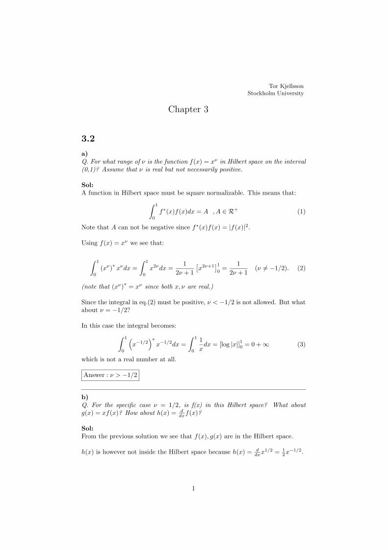
Tor KjellssonStockholm University

Chapter 3

3.2

a)Q. For what range of ν is the function f(x) = xν in Hilbert space on the interval(0,1)? Assume that ν is real but not necessarily positive.

Sol:A function in Hilbert space must be square normalizable. This means that:∫ 1

0

f∗(x)f(x)dx = A ,A ∈ R+ (1)

Note that A can not be negative since f∗(x)f(x) = |f(x)|2.

Using f(x) = xν we see that:

∫ 1

0

(xν)∗xνdx =

∫ 1

0

x2νdx =1

2ν + 1

[x2ν+1

]10

=1

2ν + 1(ν 6= −1/2). (2)

(note that (xν)∗

= xν since both x, ν are real.)

Since the integral in eq.(2) must be positive, ν < −1/2 is not allowed. But whatabout ν = −1/2?

In this case the integral becomes:∫ 1

0

(x−1/2

)∗x−1/2dx =

∫ 1

0

1

xdx = [log |x|]10 = 0 +∞ (3)

which is not a real number at all.

Answer : ν > −1/2

b)Q. For the specific case ν = 1/2, is f(x) in this Hilbert space? What aboutg(x) = xf(x)? How about h(x) = d

dxf(x)?

Sol:From the previous solution we see that f(x), g(x) are in the Hilbert space.

h(x) is however not inside the Hilbert space because h(x) = ddxx

1/2 = 12x−1/2.

1

3.3

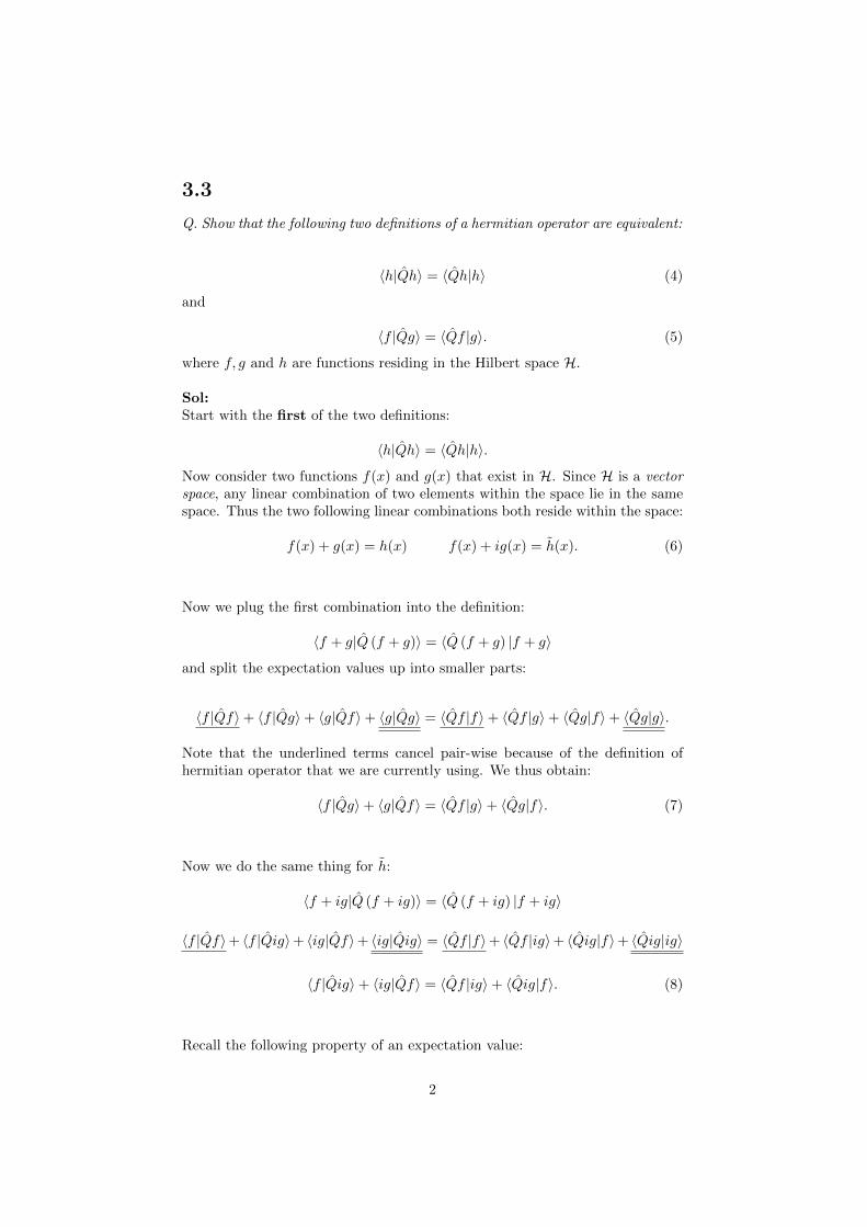
Q. Show that the following two definitions of a hermitian operator are equivalent:

〈h|Qh〉 = 〈Qh|h〉 (4)

and

〈f |Qg〉 = 〈Qf |g〉. (5)

where f, g and h are functions residing in the Hilbert space H.

Sol:Start with the first of the two definitions:

〈h|Qh〉 = 〈Qh|h〉.

Now consider two functions f(x) and g(x) that exist in H. Since H is a vectorspace, any linear combination of two elements within the space lie in the samespace. Thus the two following linear combinations both reside within the space:

f(x) + g(x) = h(x) f(x) + ig(x) = h(x). (6)

Now we plug the first combination into the definition:

〈f + g|Q (f + g)〉 = 〈Q (f + g) |f + g〉

and split the expectation values up into smaller parts:

〈f |Qf〉+ 〈f |Qg〉+ 〈g|Qf〉+ 〈g|Qg〉 = 〈Qf |f〉+ 〈Qf |g〉+ 〈Qg|f〉+ 〈Qg|g〉.

Note that the underlined terms cancel pair-wise because of the definition ofhermitian operator that we are currently using. We thus obtain:

〈f |Qg〉+ 〈g|Qf〉 = 〈Qf |g〉+ 〈Qg|f〉. (7)

Now we do the same thing for h:

〈f + ig|Q (f + ig)〉 = 〈Q (f + ig) |f + ig〉

〈f |Qf〉+ 〈f |Qig〉+ 〈ig|Qf〉+ 〈ig|Qig〉 = 〈Qf |f〉+ 〈Qf |ig〉+ 〈Qig|f〉+ 〈Qig|ig〉

〈f |Qig〉+ 〈ig|Qf〉 = 〈Qf |ig〉+ 〈Qig|f〉. (8)

Recall the following property of an expectation value:

2

〈f |cg〉 =

∫f∗(x)cg(x)dx = c

∫f∗(x)g(x)dx = c〈f |g〉

and

〈cf |g〉 =

∫(cf(x))

∗g(x)dx =

∫c∗f∗(x)g(x)dx = c∗

∫f∗(x)g(x)dx = c∗〈f |g〉

so

〈f |cg〉 = c〈f |g〉

〈cf |g〉 = c∗〈f |g〉(9)

Using this on eq.(8):

〈f |Qig〉+ 〈ig|Qf〉 = 〈Qf |ig〉+ 〈Qig|f〉

i〈f |Qg〉 − i〈g|Qf〉 = i〈Qf |g〉 − i〈Qg|f〉〈f |Qg〉 − 〈g|Qf〉 = 〈Qf |g〉 − 〈Qg|f〉. (10)

Recall now eq. (7): 〈f |Qg〉+ 〈g|Qf〉 = 〈Qf |g〉+ 〈Qg|f〉.

Adding eq. (7) to eq. (10) gives:

2〈f |Qg〉 = 2〈Qf |g〉

and hence we have arrived at the second definition of a hermitian operator:

〈f |Qg〉 = 〈Qf |g〉 (11)

and concluded that the two definitions must be equivalent.

3

3.4

a)Q. Show that the sum of two hermitian operators is also hermitian.

Sol:Let P and Q be two hermitian operators. By definition:

〈f |P f〉 = 〈P f |f〉 and 〈f |Qf〉 = 〈Qf |f〉.

Now we define K as the sum of these two operators: K = P + Q. Computingthe expectation value of K we obtain:

〈f |Kf〉 = 〈f |(P + Q)f〉 = 〈f |P f〉+ 〈f |Qf〉.

Using the hermiticity of P and Q we deduce:

〈f |Kf〉 = 〈P f |f〉+ 〈Qf |f〉 = 〈(P + Q)f |f〉 = 〈Kf |f〉 (12)

which shows that K is hermitian.

b)Q. Suppose Q is hermitian and α is a complex number. Under what conditionon α is the operator P = αQ hermitian?

Sol:Let f be a function in H. Recall that for a hermitian operator:

〈f |Qf〉 = 〈Qf |f〉.

Now we consider the left hand side (LHS) and right hand side (RHS) separatelyfor the operator P . If they are equal, then P is hermitian.

Starting with the LHS we obtain:

〈f |αQf〉 = α〈f |Qf〉 = α〈Qf |f〉. (13)

Continuing with the RHS:

〈αQf |f〉 = α∗〈Qf |f〉 = α∗〈f |Qf〉. (14)

We see that the two expressions are equal if and only if α = α∗.

The condition to put on α is that it needs to be real.

4

c)Q. When is the product of two hermitian operators hermitian?

Sol:Let P and Q be two hermitian operators, define their product as P Q = K andlet f be a function in H. Now consider the following:

〈f |Kf〉 = 〈f |P Qf〉 = 〈P f |Qf〉 = 〈QP f |f〉

so K is hermitian if and only if:

P Q = QP ⇐⇒ P Q− QP = 0 (15)

which is to say that the two operators P and Q must commute.

NoteIn general:

〈f |P g〉 = 〈P †f |g〉 (16)

where P † is called the hermitian conjugate of P . For a hermitian oper-ator we have that P † = P so what we have done until now is ok.

If you were satisfied by the solution above there is no need to read further. Forthose that however feel uneasy with the steps we include a detailed motivationbelow.

Detailed explanation on the manipulations:Since P and Q are hermitian operators the result of either of them acting on afunction f in H must also reside in H. That is to say:

Qf = g and P f = h

for some functions f,g and h in H. Therefore:

〈f |P Qf〉 = 〈f |P g〉 = 〈P f |g〉 = 〈P f |Qf〉 = 〈h|Qf〉 = 〈Qh|f〉 = 〈QP f |f〉.

5

d)Q. Show that the position operator x and the hamiltonian operator

H = − ~2

2md2

dx2 + V (x) are hermitian.

Sol:First a short remark on the position operator. When this operator acts on afunction f(x) in H it simply gives back the function multiplied by x:

xf(x) = xf(x).

Do not confuse the two things, one is the operator that does not do anythingunless it has something to operate on while the other is a unknown scalar.

Let us now check if 〈f |Qg〉 = 〈Qf |g〉:

Q = x:

〈f |xg〉 =

∫f∗(x)xg(x)dx =

∫f∗(x)xg(x)dx.

Now, a position must be real so x = x∗. Furthermore, the functions f and g arealso scalars and we know that scalar multiplication commutes (c1 · c2 = c2 · c1).Thus:∫f∗(x)xg(x)dx =

∫f∗(x)x∗g(x)dx =

∫x∗f∗(x)g(x)dx =

∫(xf(x))

∗g(x)dx

and we deduce that

〈f |xg〉 =

∫f∗(x)xg(x)dx =

∫(xf(x))

∗g(x)dx = 〈xf |g〉 (17)

so the position operator is hermitian.

Q = H:

〈f |(− ~2

2m

d2

dx2+ V (x)

)g〉 =

∫f∗(x)

(− ~2

2m

)d2

dx2g(x)dx︸ ︷︷ ︸

(1)

+

∫f∗(x)V (x)g(x)dx︸ ︷︷ ︸

(2)

In the last term, (2), if we assume the potential V (x) to be real1 we see:∫f∗(x)V (x)g(x)dx =

∫f∗(x)V ∗(x)g(x)dx =

∫(V (x)f(x))

∗g(x)dx.

that (2) is hermitian. What is left now is to check if (1) is hermitian as well.

1This is generally the case.

6

To check if (1) is hermitian we can omit the real constant factor2 to get:

〈f | d2

dx2g〉 =

∫f∗d2g

dx2dx.

To compute this we need to know the limits of the integral and since nothing isspecified we assume them to be ±∞.

Partial integration (twice) gives:

∫ ∞−∞

f∗d2g

dx2dx = f∗

dg

dx

∣∣∣∣∞−∞︸ ︷︷ ︸

0

−∫ ∞−∞

df∗

dx

dg

dxdx = − df∗

dxg

∣∣∣∣∞−∞︸ ︷︷ ︸

0

+

∫ ∞−∞

d2f∗

dx2gdx

where the underbraced terms are 0 because the functions must go to 0 at ±∞and the derivatives are finite there3. Hence we have proven that:

〈f | d2

dx2g〉 = 〈 d

2

dx2f |g〉 (18)

so the term (2) is hermitian. From 3.4a we know that the sum of two hermi-tian operators is also hermitian so the hamiltonian operator is hermitian!

Does this come as a surprise4?

2If you don’t understand why, keep the constant. After you have shown that (1) is hermi-tian, make sure you understand why the real constant factor was not important. What wouldthe case have been with an imaginary constant factor instead of a real one?

3This is the case for all physical functions at ±∞. For finite limits this need not be thecase.

4Think about what the eigenvalues of H represent.

7

3.5

The hermitian conjugate of an operator Q is the operator Q† such that:

〈f |Qg〉 = 〈Q†f |g〉 (19)

for all f and g in H. (For a hermitian operator it follows that Q† ≡ Q).

a)Q. Find the hermitian conjugates of x,i and d/dx.

Sol:Recall the following definition:

〈f |Qg〉 =

∫f∗(x)Qg(x)dx = c (20)

where c is any complex number. If an operator P has the following property:

〈P f |g〉 =

∫ (P f(x)

)∗g(x)dx = c = 〈f |Qg〉 (21)

we call it the hermitian conjugate of Q and write P ≡ Q†.

We will now use eq.(20) to look for the hermitian conjugates for the three cases.Note that the operator Q acts on g(x). The strategy is to use valid manipula-tions to remove any action on g(x) and put all on f(x) under the integral sign.Once we have managed to do so we have found, Q†.

For improved readability we drop the argument of all functions.

Q = x:

〈f |xg〉 =

∫f∗xg dx =

∫f∗xg dx =

∫(xf)

∗g dx. = 〈xf |g〉.

Here we used that x is real and that it commutes with any function.

x† = x .

Q = i:

〈f |ig〉 =

∫f∗ig dx =

∫(−if)

∗g dx. = 〈−if |g〉.

i† = −i .

8

Q = ddx:

In order to remove the derivative from g we use partial integration:⟨f

∣∣∣∣ ddxg⟩

=

∫ ∞−∞

f∗d

dxg dx = f∗g

∣∣∣∣∞−∞︸ ︷︷ ︸

0

−∫ ∞−∞

df∗

dxg dx

= −∫ ∞−∞

df∗

dxg dx =

∫ ∞−∞

(− d

dxf

)∗g dx =

⟨− d

dxf

∣∣∣∣g⟩(d

dx

)†= − d

dx

b)Q. Construct the hermitian conjugate of the harmonic oscillator raising operatora+. Recall the definition of the step operators of the harmonic oscillator:

a+ =1√

2~mω(−ip+mωx) (22)

a− =1√

2~mω(ip+mωx) (23)

Sol:Here we want to construct the hermitian conjugate of 1√

2~mω (−ip+mωx). Re-

call that:

1) The sum of two hermitian operators is also hermitian.2) We earlier proved that x is hermitian.3) −ip = −i · ~i

ddx = −~ d

dx

4)(ddx

)†= − d

dx .

From 4) it directly follows that(− ddx

)†= d

dx . We have thus found the hermitianconjugates of the two terms in a+ and therefore the hermitian conjugate of a+:

(a+)† =1√

2~mω(ip+mωx) = a− (24)

9

c)Show that (QR)† = R†Q†.

Sol:We move one operator at a time:

〈f |QRg〉 = 〈Q†f |Rg〉 (25)

and as we do that we have to exchange the operator with its hermitian conjugate(c.f problem 3.4c where we did this for hermitian operators). Now move theother operator:

〈Q†f |Rg〉 = 〈R†Q†f |g〉 (26)

and keep in mind that it has to stand all the way before everything in the bra.

From the definition of a hermitian conjugate:

〈f |QRg〉 ≡ 〈(QR)†f |g〉

and from eq.(25) and eq.(26) where we moved one operator at time:

〈f |QRg〉 = 〈R†Q†f |g〉

we see that indeed: (QR)† = R†Q†.

3.6

Q. Consider the operator Q = d2

dφ2 where φ is the azimuthal angle in polarcoordinates 0 ≤ φ ≤ 2π. The functions in H are subject to the conditionf(φ) = f(φ + 2π). Is Q hermitian? Find its eigenfunctions and eigenvalues.What is the spectrum? Is it degenerate?

Sol:Let f and g be functions in H defined on the interval (0, 2π). Let us first checkif the operator is hermitian by using partial integration to move the action fromg to f : ⟨

f

∣∣∣∣ d2dφ2 g⟩

=

∫ 2π

0

f∗d2g

dφ2dφ = f∗

dg

dφ

∣∣∣∣2π0

−∫ 2π

0

df∗

dφ

dg

dφdφ.

The first term is 0 if you assume that the derivatives are continuous, whichamounts to the condition that functions are differentiable twice. For all systemswe will consider this can be assumed and we proceed with evaluating the lastintegral:

10

⟨f

∣∣∣∣ d2dφ2 g⟩

= −∫ 2π

0

df∗

dφ

dg

dφdφ = − df∗

dφg

∣∣∣∣2π0︸ ︷︷ ︸

0

+

∫ 2π

0

d2f∗

dφ2g dφ =

⟨d2

dφ2f

∣∣∣∣g⟩

We have thus shown that our operator is hermitian.

To find its eigenfunctions and eigenvalues we now solve the eigenvalueequation for our operator:

Qf = qf

d2

dφ2f = qf

=⇒ f+ = e√qφ f− = e−

√qφ. (27)

Here f± is our eigenfunctions. The signs are used to emphasize that the func-tions are linearly independent. We will get back to this as soon as we havefound the eigenvalues q.

To find the allowed values for q we impose the boundary conditions on theeigenfunctions:

e±√qφ = e±

√q(φ+2π)

1 = e±√q(2π)

ein2π = e±√q(2π) ∀n ∈ Z (28)

This sets the condition on q:

q = −n2 ∀n ∈ Zq = 0,−1,−4,−9 . . .

The set of allowed values for q is called the spectrum of the operator. Fromeq.(27) we see that for each value of q except 0 there are two distincteigenfunctions, f+ and f− so for these values of q the spectrum is doubly de-generate.

For q = 0 we see that f+ = f− so there is no degeneracy in this case.

11

3.7

a)Q. Suppose that f(x) and g(x) are two eigenfunctions of an operator Q, withthe same eigenvalue q. Show that any linear combination of f and g is itself aneigenfunction of Q with the eigenvalue q.

Sol:We want to show that if the following is true:

Qf = qf and Qg = qg (29)

then for any complex numbers c1, c2 it follows that:

Q(c1f + c2g) = q(c1f + c2g).

This is very straightforward. Since c1, c2 are just numbers, Q has no effect onthem:

Q(c1f + c2g) = Qc1f + Qc2g = c1Qf + c2Qg

From (29) we see:

c1Qf + c2Qg = c1qf + c2qg = q(c1f + c2g)

and hence:

Q(c1f + c2g) = q(c1f + c2g)

12

b)Q. Check that f(x) = ex and g(x) = e−x are eigenfunctions of the operatord2/dx2, with the same eigenvalue. Construct two linear combinations of f andg that are orthogonal eigenfunctions on the interval (-1,1).

Sol:Apply the operator to the functions and you get:

d2

dx2e±x = e±x

so indeed they have the same eigenvalue (q = 1).

Now we want to construct two linear combination of these that are orthogonalon the interval (-1,1). If we name them:

h1 = a1ex + b1e

−x and h2 = a2ex + b2e

−x (30)

we have that they are orthogonal on the interval (-1,1) if:∫ 1

−1h∗1h2 dx = 0.∫ 1

−1a∗1a2e

2x + b∗1a2 + a∗1b2 + b∗1b2e−2x dx = 0

1

2a∗1a2(e2 − e−2) + 2(b∗1a2 + a∗1b2) +

1

2b∗1b2(e2 − e−2) = 0. (31)

For this equation to hold we need to put constraints on the coefficients a1, a2, b1and b2. Since we are only asked to give an example we can put whatever valueswe want5.

By this sneaky choice:a∗1a2 = −b∗1b2

we make the first and third term in eq.(31) kill each other. Thus we now have:

2(b∗1a2 + a∗1b2) = 0. (32)

To make our lives even easier we choose all coefficients to be real.

Our two choices thus far have now given us the following conditions that wemust obey:

a1a2 = −b1b2b1a2 = −a1b2.

(33)

From here there is no fancy thinking - any combination will do. One easy com-bination is a1 = a2 = b1 = 1 and b2 = −1.

With this choice h1, h2 become:

h1 = ex + e−x h2 = ex − e−x (34)

which are a multiples of the functions cosh(x) and sinh(x).

5You could in principle try to use the Gram-Schmidt, but don’t.

13

3.8

a)Q. Let H denote the Hilbert space of all functions subject to the conditionf(φ) = f(φ + 2π) and let 0 ≤ φ ≤ 2π. Check that the eigenvalues of thehermitian operator i ddφ are real. Also, show that the eigenfunctions for distincteigenvalues are orthogonal.

Sol:The eigenvalue equation for this is:

id

dφf = qf =⇒ f = Ae−iqφ (35)

which, like before, is the general solution of the differential equation. Just likethe previous problem we get a condition on the eigenvalues from the periodicityof the functions:

e−iqφ = e−iq(φ+2π) =⇒ −iq2π = 2πn ∀n ∈ Z =⇒ q = n ∀n ∈ Z

so the eigenvalues are indeed real.

Now we explicitly verify that two eigenfunctions, fa and fb, with distinct eigen-values a 6= b, are orthogonal:

〈fa|fb〉 =

∫ 2π

0

(e−iaφ

)∗e−ibφ dφ =

∫ 2π

0

ei(a−b)φ dφ =1

i(a− b)[ei(a−b)2π︸ ︷︷ ︸

1

−1]

= 0

where the last underbrace holds because both a and b are integers.

b)Q. Now do the same for the operator in Problem 3.6.

Sol:In problem 3.6 we saw that the eigenfunctions were:

f± = e±√qφ (36)

with eigenvalues:q = 0,−1,−4,−9 . . .

so we immeditely see that the eigenvalues are real. Furthermore, since√q = iα

for a (non-negative integer) α, these eigenfunctions are the same as in problem3.8a and any property proved there need not be proved again.

14

3.10

Q. Is the ground state of the infinite square well an eigenfunction of the mo-mentum operator? If so, what is its momentum? If not, why not?

Sol:If the ground state of the infinite square well:

ψ1(x) =

√2

asin(πxa

)(37)

is an eigenfunction of the momentum operator p, then pψ1(x) = A · ψ1(x) forsome complex constant A. Now we check if this is the case:

pψ1(x) = id

dxψ1(x) = i

π

a

√2

acos(πxa

).

so:pψ1(x) 6= Aψ1(x).

ψ1(x) is not an eigenfunction of the momentum operator.

15

3.13

a)Q. Prove the following commutator identity:

[AB, C] = A[B, C] + [A, C]B

Sol:We start by expanding the two commutators on the right hand side and forbrevity we drop the hats:

A[B,C] + [A,C]B = (ABC −ACB) + (ACB − CAB) =

A[B,C] + [A,C]B = ABC − CAB = [AB,C]

which is what we were asked to prove.

b) Q. Show that [xn, p] = i~nxn−1Sol:This problem can be solved either by:1) using the previous problem.2) using the technique with test functions, as in the next problem6.

In this solution we choose option (1). First expand the commutator [xn, p] usingthe rule you proved in the previous problem:

[xn, p] = [x · xn−1, p] = x[xn−1, p] + [x, p]xn−1 = x[xn−1, p] + i~xn−1

where we have used [xn, p] = i~. There will soon be an explanation to why thelast term is underlined.

Now we evaluate x[xn−1, p] by once again expanding the commutator:

x[xn−1, p] = x(x[xn−2, p] + [x, p]xn−2

)=

= x(x[xn−2, p] + i~xn−2

)= x2[xn−2, p] + i~xn−1

observe that we once again got a term i~xn−1.

Focus now on the first term. This term will obviously survive the same procedureuntil the commutator is 0:

[x0, p] = [1, p] = 0.

To reach this commutator starting from [xn, p] we see that we need to apply theprocedure n times. This means:

[xn, p] = x[xn−1, p] + i~xn−1 =

/iterate n times

/=

0 + i~xn−1 + . . .+ i~xn−1︸ ︷︷ ︸n elements

= i~nxn−1. �

6Thanks to Jonathan Klasen for highlighting this!

16

c)Q. Show more generally that

[f(x), p] = i~df

dx

for any function f(x).

Sol:Here we will need to use the explicit form of the momentum operator. When-ever you do this it is best to have a test function to work with, otherwise theprobability of creating a mess is high. Let g(x) be such a test function and letthe commutator work on it:

[f(x), p]g(x) = f(x)pg(x)− pf(x)g(x)

= f(x)

(~i

d

dx

)g(x)−

(~i

d

dx

)f(x)g(x)

=~i

[f(x)

dg

dx−(df

dxg(x) +

dg

dxf(x)

)]= −~

i

df

dxg(x)

Now that the test function g(x) has fulfilled its purpose it can be thrown away:

[f(x), p] = i~df

dx. (38)

3.14

Q. Prove the famous ”(your name) uncertainty principle”, relating the uncer-tainty in position (A = x) to the uncertainty in energy H = p2/2m+ V :

σxσH ≥~

2m|〈p〉|

For stationary states this doesn’t tell you much - why not?

Sol:Recall the generalized uncertainty principle (derived in section 3.5):

σ2Aσ

2B ≥

(1

2i〈[A, B]〉

)2

(39)

We would like to apply this to our two operators. To do this, we must firstevaluate the commutator [x, H]:

17

[x, H] = [x, p2/2m+ V (x)] = [x, p2/2m] + [x, V (x)]︸ ︷︷ ︸0

Here we have used:[A, B + C] = [A, B] + [A, C] (40)

which is easy to prove (do it as an exercise) and that x commutes with anyfunction of x, such as V (x).

Now we will focus on the first commutator and start by rewriting it7

[x, p2/2m] =1

2m[x, p2] = − 1

2m[p2, x]

and then expanding this using the result from 3.13a:

[x, p2/2m] = − 1

2m[p2, x] = − 1

2m(p[p, x] + [p, x]p) =

1

2m(2 (i~) p)

[x, p2/2m] = i~p

m. (41)

Taking the expectation value of eq.(41) and inserting it into eq.(39) gives:

σxσH ≥∣∣∣∣ 1

2ii~〈p〉m

∣∣∣∣ =~

2m|〈p〉|. (42)

Note: we dropped the hat in the last equality because in our notation 〈Q〉 = 〈Q〉

Finally, regarding the question of stationary states:1) For stationary states the spread in energy, σH , is zero.2) Since every expectation value is constant in time 〈x〉 is constant and hence

〈p〉 = md〈x〉dt = 0. From eq. (42) we then obtain: 0 ≥ 0.

7Here we are using two other properties: [αA, B] = [A, αB] = α[A, B] and [A, B] = −[A, B]which are easy to prove.

18

3.17

Q. Apply eq. (3.71) (the equation is a measure of how fast a system is changing):

d

dt〈Q〉 =

i

~〈[H, Q]〉+

⟨∂Q

∂t

⟩to the following special cases:a) Q = 1b) Q = Hc) Q = xd) Q = p.

In each case, comment on the result, with particular reference to eq. (1.27),(1.33), (1.38) and the discussion on the conservation of energy following eq.(2.39) in the textbook.

Sol:

a)

d

dt〈1〉 =

i

~〈[H, 1]〉︸ ︷︷ ︸

0

+

⟨∂1

∂t

⟩︸ ︷︷ ︸

0

(a scalar commutes with everything) so the left hand side must be 0. Recallthat:

〈1〉 = 〈Ψ|1|Ψ〉 =

∫ ∞−∞|Ψ|2dx (43)

so this is exactly the result in eq. (1.27) in the textbook:

d

dt

∫ ∞−∞|Ψ(x, t)|2dx︸ ︷︷ ︸〈1〉

= 0.

b)

d

dt〈H〉 =

i

~〈[H, H]〉︸ ︷︷ ︸

0

+

⟨∂H

∂t

⟩.

The first term on the right hand side is 0 because every operator commutes withitself. Assuming that the Hamiltonian is independent of time the last term isalso 0. Thus we read:

d

dt〈H〉 = 0. (44)

19

which is the statement of conservation of energy. (in the textbook this is pre-sented right after eq. (2.39)).

c)

d

dt〈x〉 =

i

~〈[H, x]〉+

⟨∂x

∂t

⟩︸ ︷︷ ︸

0

.

Recall that H = p2

2m + V (x) so:

[H, x] = −[x, H] = − i~pm

where we used the answer from problem 3.14.

Thus we get:

d

dt〈x〉 = − i

~

⟨i~pm

⟩=〈p〉m.

which is eq. (1.33) in the textbook.

d)

d

dt〈p〉 =

i

~〈[H, p]〉+

⟨∂p

∂t

⟩︸ ︷︷ ︸

0

where the last term is 0 since the momentum operator does not have a time-

dependence. Using H = p2

2m + V (x) and the fact that operators (and powers ofthem) commute with themselves we now obtain:

d

dt〈p〉 =

i

~〈[V (x), p]〉.

Focusing on the commutator and using the result in problem 3.13 c) we obtain:

[V (x), p] = i~dV

dx

so re-inserting this we get:

d

dt〈p〉 = −

⟨dV

dx

⟩which is eq. (1.38) in the textbook, an instance of Ehrenfest’s theorem (andso is the previous problem). This theorem states that expectation values followclassical laws. Do you recognize the equation above? (Hint: −dVdx = F )

20

3.22

Q. Consider a three-dimensional vector space spanned by an orthonormal basis|1〉, |2〉, |3〉. The two kets |α〉, |β〉 are given by:

|α〉 = i|1〉 − 2|2〉 − i|3〉 and |β〉 = i|1〉+ 2|3〉.

a)Q. Construct 〈α| and 〈β| in terms of the dual basis vectors 〈1|, 〈2|, 〈3|.

Sol:This is very easy, just remember that the constants are now given by the complexconjugate of the constants in front of the kets:

〈α| = −i〈1| − 2〈2|+ i〈3| (45)

〈β| = −i〈1|+ 2〈3| (46)

b)Q. Find 〈α|β〉 and 〈β|α〉 and confirm that 〈α|β〉 = 〈β|α〉∗.

Sol:

〈α|β〉 =(− i〈1| − 2〈2|+ i〈3|

)(i|1〉+ 2|3〉

)=

−i · i 〈1|1〉︸︷︷︸1

−i · 2 〈1|3〉︸︷︷︸0

−2 · i 〈2|1〉︸︷︷︸0

−2 · 2 〈2|3〉︸︷︷︸0

+i · i 〈3|1〉︸︷︷︸0

+i · 2 〈3|3〉︸︷︷︸1

= 1 + 2i

where the brakets are either 0 (orthonormal basis) or 1 (orthonormal basis).Now we do the same for 〈β|α〉:

〈β|α〉 =(− i〈1|+ 2〈3|

)(i|1〉 − 2|2〉 − i|3〉

)=

−i·i 〈1|1〉︸︷︷︸1

−i·(−2) 〈1|2〉︸︷︷︸0

−i·(−i) 〈1|3〉︸︷︷︸0

+2·i 〈3|1〉︸︷︷︸0

+2·(−2) 〈3|2〉︸︷︷︸0

+2·(−i) 〈3|3〉︸︷︷︸1

= 1−2i

and we indeed see that 〈α|β〉 = 〈β|α〉∗ as it should.

c)Q. Find all nine matrix elements of the operator A = |α〉〈β| in this basis andthen write A on matrix form. Is it hermitian?

Sol:In a given basis we find the matrix elements of an operator by computing:

Aab = 〈a|A|b〉

21

where a, b are labels of the basis vectors8. Before explicitly showing the stepsmake a short comment on the notation:

Aab = 〈a||α〉〈β||b〉

will be written asAab = 〈a|α〉〈β|b〉.

Let us now start computing the matrix elements, which at start will be shownin detail:

A11 = 〈1|α〉〈β|1〉 =

[〈1|(i|1〉 − 2|2〉 − i|3〉

)︸ ︷︷ ︸α

][ (− i〈1|+ 2〈3|

)︸ ︷︷ ︸β

|1〉]

we see that the matrix elements become products of two brakets. Rememberthat the basis is orthonormal, this saves you some time because 〈i|j〉 = 0 ifi 6= j. Thus:

A11 = 〈1|α〉〈β|1〉 =

[〈1|(i|1〉 − 2|2〉 − i|3〉

)︸ ︷︷ ︸α

][ (− i〈1|+ 2〈3|

)︸ ︷︷ ︸β

|1〉]

=

[i〈1|1〉

][− i〈1|1〉

]= i · (−i) = 1

(also, remember that the basis is normalized (orthonormal basis) so 〈i|i〉 = 1.)

Now we compute A12:

A12 = 〈1|α〉〈β|2〉 =

[〈1|(i|1〉 − 2|2〉 − i|3〉

)][(− i〈1|+ 2〈3|

)|2〉]

The first square bracket here is the same as before since it is only 〈1|α〉 whichwe computed before; 〈1|α〉 = i. Continuing with the algebra:

A12 = i

[(− i〈1|+ 2〈3|

)|2〉]

= i

[0

]= 0

where the second square bracket is 0 because the bras are 〈1| and 〈3| but theket is |2〉 so the products of these will be 0.

Now we do the same for A13:

A13 = 〈1|α〉〈β|3〉 =

[〈1|(i|1〉 − 2|2〉 − i|3〉

)][(− i〈1|+ 2〈3|

)|3〉]

= i

[(− i〈1|+ 2〈3|

)|3〉]

= i

[2〈3|3〉

]= 2i

8It is also common to write the basis kets as |ea〉, |eb〉 - don’t be fooled by the notation.

22

Computing the rest is really just the same algebraic steps all over again. There-fore we only list the results:

A21 = 〈2|α〉〈β|1〉 = −2·(−i), A22 = 〈2|α〉〈β|2〉 = −2·0, A23 = 〈2|α〉〈β|3〉 = −2·2

A31 = 〈3|α〉〈β|1〉 = −i·(−i), A32 = 〈3|α〉〈β|2〉 = −i·0, A33 = 〈3|α〉〈β|3〉 = −i·2

As you see, even if you have to compute nine matrix elements a lot of them havemuch in common. Now, writing this out in matrix form yields:

A =

1 0 2i2i 0 −4−1 0 −2i

.

To check if this is hermitian we need to see if A = A†. In this case it is nothard, you could just transpose it and then complex conjugate it to see that theresult is not A. But there is an even faster way - there cannot be any imaginarynumbers in the diagonal!9 So assume you had a 100× 100 matrix instead, thenyou definitely check the diagonal first.

9This is rooted in the definition of hermitian operators: the diagonal remains the sameafter computing the transpose so if there are imaginary numbers you can never get the samebefore and after the complex conjugation.

23

3.23

Q. The Hamiltonian for a certain two-level system is:

H = ε[|1〉〈1| − |2〉〈2|+ |1〉〈2|+ |2〉〈1|

]where |1〉, |2〉 forms an orthonormal basis and ε is a number with the dimensionof energy. Find its eigenvalues and eigenvectors (as linear combinations of |1〉and |2〉). What is the matrix representation H of H in this basis?

Sol:You could answer all questions by computing the matrix elements of H and thensolve the matrix eigenvalue equation. We will however first use a way that onlyuses Dirac notation and then after that present the solution using the matrixnotation.

Method 1: Using Dirac notation

We are asked to give the eigenvectors of the operator

H = ε[|1〉〈1| − |2〉〈2|+ |1〉〈2|+ |2〉〈1|

]which means that we want to solve the eigenvalue equation:

H|α〉 = λ|α〉

for some scalars λ and non-zero eigenvectors |α〉. To start with we define:

|α〉 = c1|1〉+ c2|2〉 c1, c2 ∈ C

which just means that we express the eigenvectors in the basis given.

Now we plug this into the eigenvalue equation:

H[c1|1〉+ c2|2〉

]= λ

[c1|1〉+ c2|2〉

]and insert H defined in terms of the basis:

ε[|1〉〈1| − |2〉〈2|+ |1〉〈2|+ |2〉〈1|

][c1|1〉+ c2|2〉

]= λ

[c1|1〉+ c2|2〉

].

The left hand side can be simplified in the following manner:

ε[|1〉〈1| − |2〉〈2|+ |1〉〈2|+ |2〉〈1|

][c1|1〉+ c2|2〉

]=

ε

[c1|1〉 〈1|1〉︸︷︷︸

1

−c1|2〉 〈2|1〉︸︷︷︸0

+c1|1〉 〈2|1〉︸︷︷︸0

+c1|2〉 〈1|1〉︸︷︷︸1

+

c2|1〉 〈1|2〉︸︷︷︸0

−c2|2〉 〈2|2〉︸︷︷︸1

+c2|1〉 〈2|2〉︸︷︷︸1

+c2|2〉 〈1|2〉︸︷︷︸0

]and we see that our eigenvalue equation now has taken the following form:

24

ε[c1|1〉+ c1|2〉 − c2|2〉+ c2|1〉

]= λ

[c1|1〉+ c2|2〉

]which gives the following system of equations:

ε(c1 + c2) = λc1ε(c1 − c2) = λc2

=⇒ c2 = c1(λε − 1)c2 = c1(λε + 1)−1

Equating the two rows we can find our eigenvalues:

λ

ε− 1 = (

λ

ε+ 1)−1

λ2

ε2− 1 = 1

λ2 = 2ε2

λ = ±√

2ε . (47)

Inserting the eigenvalues into our expression for the coefficients c1, c2 we ob-tain10:

c2 = c1(λ

ε− 1) = c1(

±√

2ε

ε− 1) = c1(±

√2− 1)

which gives us two eigenvectors:

|α±〉 = c1|1〉+ c1(±√

2− 1)|2〉 . (48)

If we also want to normalize the vectors we must choose11

c1 =1√

12 + (±√

2− 1)2.

10Any of the two lines work.11If you don’t see why, it is a good exercise to explicitly do this. You find c1 by computing〈α±|α±〉 and by requiring that this should be 1 you get what c1 must be.

25

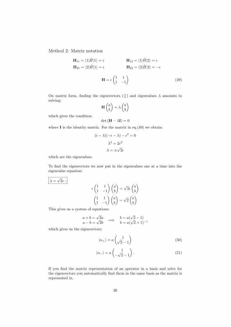
Method 2: Matrix notation

H11 = 〈1|H|1〉 = ε H12 = 〈1|H|2〉 = ε

H21 = 〈2|H|1〉 = ε H22 = 〈2|H|2〉 = −ε

H = ε

(1 11 −1

)(49)

On matrix form, finding the eigenvectors ( ab ) and eigenvalues λ amounts tosolving:

H

(ab

)= λ

(ab

)which gives the condition:

det (H− λI) = 0

where I is the identity matrix. For the matrix in eq.(49) we obtain:

(ε− λ)(−ε− λ)− ε2 = 0

λ2 = 2ε2

λ = ±√

2ε

which are the eigenvalues.

To find the eigenvectors we now put in the eigenvalues one at a time into theeigenvalue equation:

λ =√

2ε :

ε

(1 11 −1

)(ab

)=√

2ε

(ab

)(

1 11 −1

)(ab

)=√

2

(ab

)This gives us a system of equations:

a+ b =√

2a

a− b =√

2b=⇒ b = a(

√2− 1)

b = a(√

2 + 1)−1

which gives us the eigenvectors:

|α+〉 = a

(1√

2− 1

)(50)

|α−〉 = a

(1

−√

2− 1

). (51)

If you find the matrix representation of an operator in a basis and solve forthe eigenvectors you automatically find them in the same basis as the matrix isrepresented in.

26

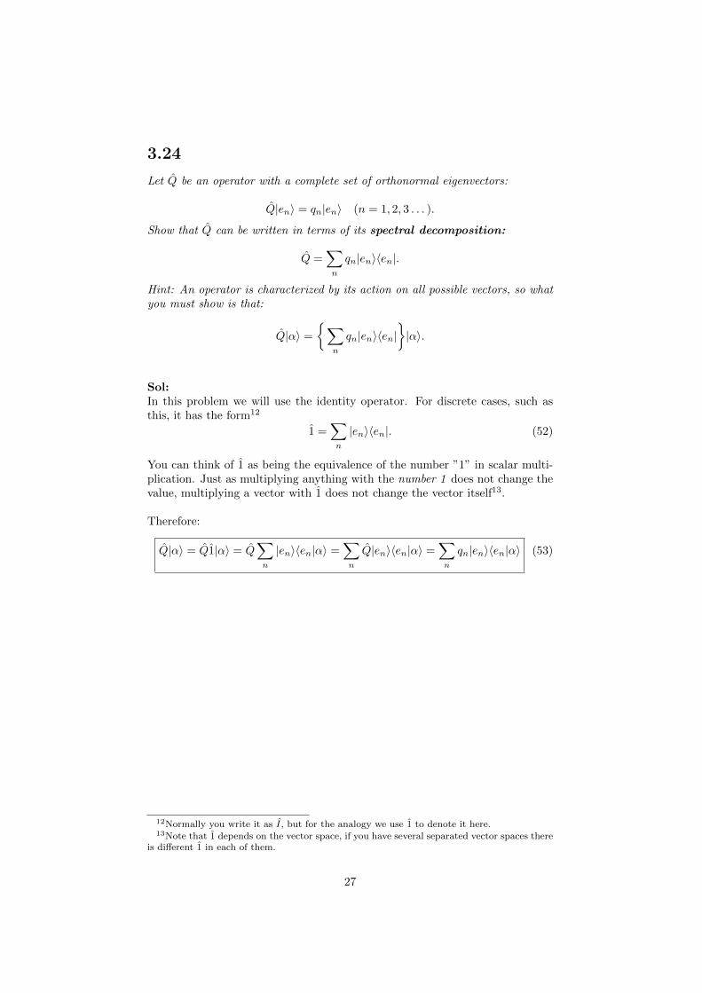
3.24

Let Q be an operator with a complete set of orthonormal eigenvectors:

Q|en〉 = qn|en〉 (n = 1, 2, 3 . . . ).

Show that Q can be written in terms of its spectral decomposition:

Q =∑n

qn|en〉〈en|.

Hint: An operator is characterized by its action on all possible vectors, so whatyou must show is that:

Q|α〉 =

{∑n

qn|en〉〈en|}|α〉.

Sol:In this problem we will use the identity operator. For discrete cases, such asthis, it has the form12

1 =∑n

|en〉〈en|. (52)

You can think of 1 as being the equivalence of the number ”1” in scalar multi-plication. Just as multiplying anything with the number 1 does not change thevalue, multiplying a vector with 1 does not change the vector itself13.

Therefore:

Q|α〉 = Q1|α〉 = Q∑n

|en〉〈en|α〉 =∑n

Q|en〉〈en|α〉 =∑n

qn|en〉〈en|α〉 (53)

12Normally you write it as I, but for the analogy we use 1 to denote it here.13Note that 1 depends on the vector space, if you have several separated vector spaces there

is different 1 in each of them.

27

3.27

Q. Sequential measurements. An operator A, representing observable A, hastwo normalized eigenstates ψ1 and ψ2, with eigenvalues a1 and a2 respectively.Operator B, representing the observable B, has two normalized eigenstates φ1and φ2, with eigenvalues b1 and b2. The eigenstates are related by:

ψ1 = (3φ1 + 4φ2)/5 and ψ2 = (4φ1 − 3φ2)/5. (54)

a)Q. Observable A is measured and the value a1 is obtained. What is the state ofthe system (immediately) after this measurement?

Sol:Before the measurement is done there is only a probability that the object willbe found in a certain eigenstate. When you perform the measurement and findit in a given state (by measuring the related observable) it will stay in thatstate until the wave function evolves. Since this evolution is not immediate the

answer is ψ1 .

b)Q. If B is measured now, what are the possible results and what are their prob-abilities?

Sol:The particle is in the state ψ1. If we measure B we can only obtain the eigen-values of B: b1 or b2.

To find the probabilities we must express ψ1 in terms of the eigenstates of B:

ψ1 = c1φ1 + c2φ2 =3

5φ1 +

4

5φ2. (55)

The probabilities to obtain b1 or b2 are given by |c1|2 and |c2|2:

Result Probabilityb1 9/25b2 16/25

28

c)Q. Right after the measurement of B, A is measured again. What is the proba-bility of getting a1? (Note that the answer would be quite different if you weretold what the measurement of B in the previous problem gave.)

Sol:Remember, the measurement of B put the state in one of the eigenstate of B:φ1 or φ2. If A is measured now, the probability to get a1 depends on which ofthese the state was put in:

If the state is in φ1:First we must express φ1 in terms of ψ1, ψ2. This is done by inverting eq.(54):

φ1 = (3ψ1 + 4ψ2)/5 (56)

If A is measured now, the probability to get a1 is: 925 .

If the state is in φ2:

φ2 = (4ψ1 − 3ψ2)/5. (57)

If A is measured now, the probability to get a1 is: 1625 .

The probability that we get a1 now if the previous measurement on Bgave b1 is:

P (b1, a1) =9

25· 9

25.

The probability that we get a1 now if the previous measurement on Bgave b2 is:

P (b2, a1) =16

25· 16

25

so the total probability of getting a1 if the previous measurement of B isunknown is:

Ptot(a1) = P (b1, a1) + P (b2, a1) ≈ 0.539

29

3.31

(The problem is split into three parts.)

Virial theorem. Apply:

d

dt〈Q〉 =

i

~〈[H, Q]〉+

⟨∂Q

∂t

⟩to show that:

d

dt〈xp〉 = 2〈T 〉 −

⟨xdV

dx

⟩. (58)

where T is the kinetic energy p2

2m .

Sol:Let us start with noting that there is no explicit time dependence in our oper-ator: Q = xp = x~

iddx : ⟨

∂Q

∂t

⟩=

⟨∂xp

∂t

⟩= 0

which gives:d

dt〈xp〉 =

i

~〈[H, xp]〉. (59)

Focus now on the commutator [H, xp]. In problem 3.13 we proved:

[AB, C] = A[B, C] + [A, C]B

which we will now use:

[H, xp] = −[xp, H] = −(x[p, H] + [x, H]p

)= x[H, p] + [H, x]p.

From problem 3.17 we read:

[H, x] = − i~pm

[H, p] =

[p2

2m+ V (x), p

]= −

[p2

2m, p

]︸ ︷︷ ︸

0

−[V (x), p] = −i~dVdx

Inserting this into eq. (59) gives:

d

dt〈xp〉 =

i

~〈[H, xp]〉 =

i

~

⟨− i~p2

m+ i~x

dV

dx

⟩=

⟨p2

m

⟩−⟨xdV

dx

⟩= 2〈T 〉 −

⟨xdV

dx

⟩

30

Q. Why isd

dt〈xp〉 = 0. (60)

in a stationary state?

Sol:In a stationary state every expectation value is constant in time.

Q. The relation:

2〈T 〉 =

⟨xdV

dx

⟩(61)

is called the virial theorem. Use it to prove that 〈T 〉 = 〈V 〉 for stationarystates of the harmonic oscillator and check that this is consistent with the re-sults you got in problems 2.11 and 2.12.

Sol:For the harmonic oscillator, the potential is given by:

V (x) =1

2mω2x2

so inserting this into eq. (58) gives:

d

dt〈xp〉 = 2〈T 〉 − 〈mω2x2〉 = 2〈T 〉 − 2〈V 〉. (62)

For any stationary state all expectation values are constant in time, so the leftside above is 0. Thus:

〈T 〉 = 〈V 〉 (63)

and we have just shown what we were asked to show.

The result is consistent with what was found in problem 2.11 c) and 2.12 where〈T 〉 and 〈V 〉 were explicitly computed.

31