Chapter 3 3 - Atomic Theorykjellsson/teaching/QMII/chapt3_sol_tor.pdf · Tor Kjellsson Stockholm...
35
Tor Kjellsson Stockholm University Chapter 3 3.2 a) Q. For what range of ν is the function f (x)= x ν in Hilbert space on the interval (0,1)? Assume that ν is real but not necessarily positive. Sol: A function in Hilbert space is always normalizable. This means that: Z 1 0 f * (x)f (x)dx = A (1) where A is a real number. Note also that this number can not be negative since f * (x)f (x)= |f (x)| 2 . Using this for our function we obtain: Z 1 0 x 2ν dx = 1 2ν +1 x 2ν+1 1 0 = 1 2ν +1 (2) under the assumption that ν 6= -1/2 which is a case that we have to study separately. Now, since the LHS of eq.(2) is non-negative we obtain: ν> -1/2. But what about ν = -1/2? In this case we obtain: Z 1 0 1 x dx = [log |x|] 1 0 =0+ ∞ (3) which is not normalizable. Answer : ν> -1/2 b) Q. For the specific case ν =1/2, is f(x) in this Hilbert space? What about g(x)= xf (x)? How about h(x)= d dx f (x)? Sol: f (x),g(x) are obviously in the Hilbert space since we proved that x ν for all ν> -1/2 reside in the space. h(x) however does not live inside the Hilbert space because h(x)= d dx x 1/2 = 1 2 x -1/2 and we earlier proved that this is not a normalizable function. 1
-
Upload
truongliem -
Category
Documents
-
view
240 -
download
0
Transcript of Chapter 3 3 - Atomic Theorykjellsson/teaching/QMII/chapt3_sol_tor.pdf · Tor Kjellsson Stockholm...
Tor KjellssonStockholm University
Chapter 3
3.2
a)Q. For what range of ν is the function f(x) = xν in Hilbert space on the interval(0,1)? Assume that ν is real but not necessarily positive.
Sol:A function in Hilbert space is always normalizable. This means that:∫ 1
0
f∗(x)f(x)dx = A (1)
where A is a real number. Note also that this number can not be negative sincef∗(x)f(x) = |f(x)|2.
Using this for our function we obtain:∫ 1
0
x2νdx =1
2ν + 1
[x2ν+1
]10
=1
2ν + 1(2)
under the assumption that ν 6= −1/2 which is a case that we have to studyseparately. Now, since the LHS of eq.(2) is non-negative we obtain: ν > −1/2.But what about ν = −1/2?
In this case we obtain: ∫ 1
0
1
xdx = [log |x|]10 = 0 +∞ (3)
which is not normalizable.
Answer : ν > −1/2
b)Q. For the specific case ν = 1/2, is f(x) in this Hilbert space? What aboutg(x) = xf(x)? How about h(x) = d
dxf(x)?
Sol:f(x), g(x) are obviously in the Hilbert space since we proved that xν for allν > −1/2 reside in the space. h(x) however does not live inside the Hilbertspace because h(x) = d
dxx1/2 = 1
2x−1/2 and we earlier proved that this is not a
normalizable function.
1
3.3
Q. Show that the following two definitions of a hermitian operator are equivalent:
〈h|Qh〉 = 〈Qh|h〉 (4)
and
〈f |Qg〉 = 〈Qf |g〉. (5)
where f, g and h are functions residing in Hilbert space H.
Sol:Start with the first of the two definitions:
〈h|Qh〉 = 〈Qh|h〉.
Now consider two functions f(x) and g(x) that exist in H. Since H is a vectorspace, any linear combination of two elements within the space lie in the samespace. Thus the two following linear combinations both reside within the space:
f(x) + g(x) = h(x) f(x) + ig(x) = h(x). (6)
Now we plug the first combination into the definition:
〈f + g|Q (f + g)〉 = 〈Q (f + g) |f + g〉
and split the expectation values up into smaller parts:
〈f |Qf〉+ 〈f |Qg〉+ 〈g|Qf〉+ 〈g|Qg〉 = 〈Qf |f〉+ 〈Qf |g〉+ 〈Qg|f〉+ 〈Qg|g〉.
Note that the underlined terms cancel pair-wise because of the definition ofhermitian operator that we are currently using. We thus obtain:
〈f |Qg〉+ 〈g|Qf〉 = 〈Qf |g〉+ 〈Qg|f〉. (7)
Now we do the same thing for h:
〈f + ig|Q (f + ig)〉 = 〈Q (f + ig) |f + ig〉
〈f |Qf〉+ 〈f |Qig〉+ 〈ig|Qf〉+ 〈ig|Qig〉 = 〈Qf |f〉+ 〈Qf |ig〉+ 〈Qig|f〉+ 〈Qig|ig〉
〈f |Qig〉+ 〈ig|Qf〉 = 〈Qf |ig〉+ 〈Qig|f〉. (8)
Recall the following property of an expectation value:
2
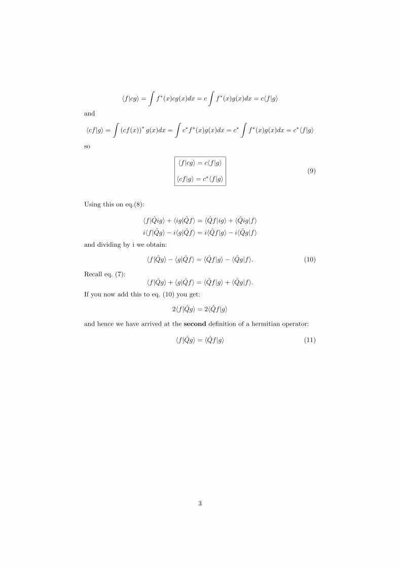
〈f |cg〉 =
∫f∗(x)cg(x)dx = c
∫f∗(x)g(x)dx = c〈f |g〉
and
〈cf |g〉 =
∫(cf(x))
∗g(x)dx =
∫c∗f∗(x)g(x)dx = c∗
∫f∗(x)g(x)dx = c∗〈f |g〉
so
〈f |cg〉 = c〈f |g〉
〈cf |g〉 = c∗〈f |g〉(9)
Using this on eq.(8):
〈f |Qig〉+ 〈ig|Qf〉 = 〈Qf |ig〉+ 〈Qig|f〉
i〈f |Qg〉 − i〈g|Qf〉 = i〈Qf |g〉 − i〈Qg|f〉
and dividing by i we obtain:
〈f |Qg〉 − 〈g|Qf〉 = 〈Qf |g〉 − 〈Qg|f〉. (10)
Recall eq. (7):〈f |Qg〉+ 〈g|Qf〉 = 〈Qf |g〉+ 〈Qg|f〉.
If you now add this to eq. (10) you get:
2〈f |Qg〉 = 2〈Qf |g〉
and hence we have arrived at the second definition of a hermitian operator:
〈f |Qg〉 = 〈Qf |g〉 (11)
3
3.4
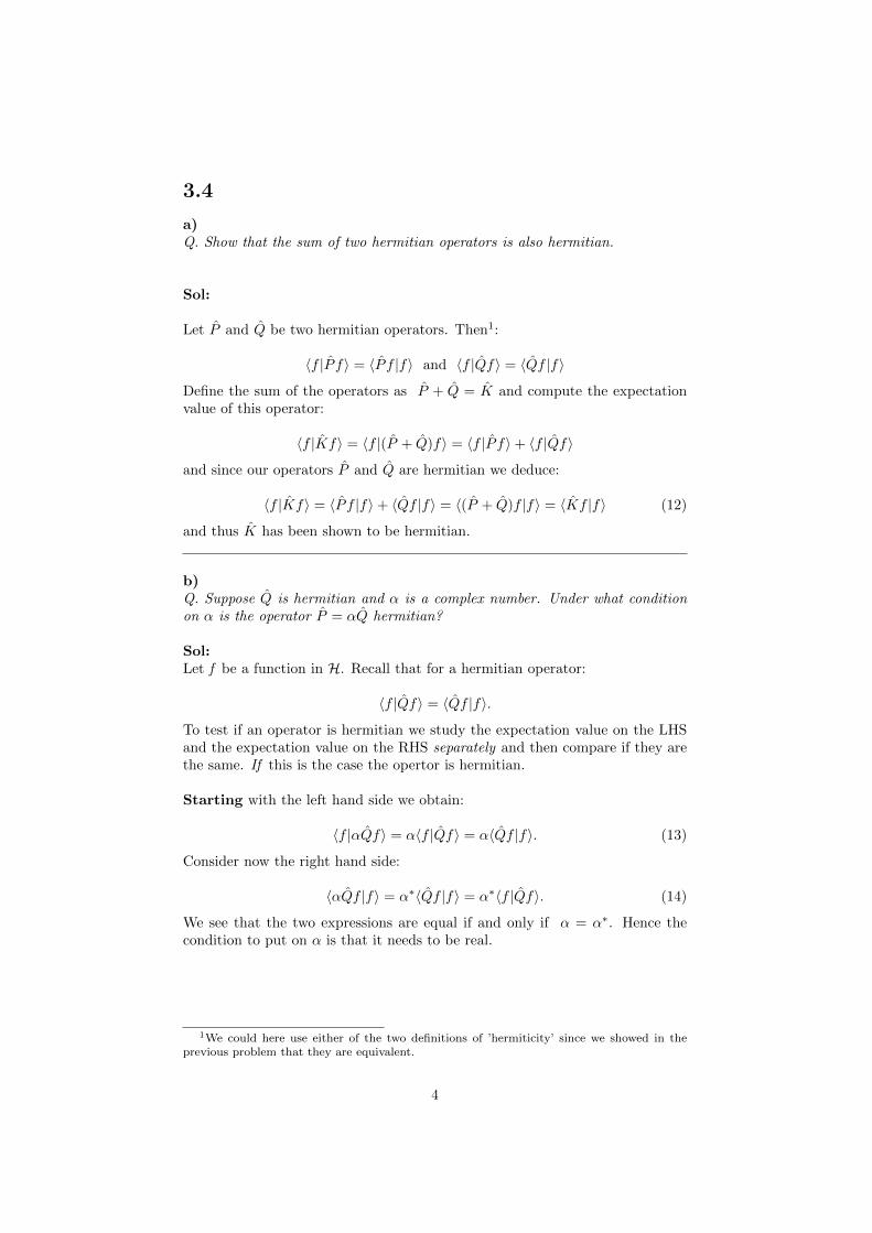
a)Q. Show that the sum of two hermitian operators is also hermitian.
Sol:
Let P and Q be two hermitian operators. Then1:
〈f |P f〉 = 〈P f |f〉 and 〈f |Qf〉 = 〈Qf |f〉
Define the sum of the operators as P + Q = K and compute the expectationvalue of this operator:
〈f |Kf〉 = 〈f |(P + Q)f〉 = 〈f |P f〉+ 〈f |Qf〉
and since our operators P and Q are hermitian we deduce:
〈f |Kf〉 = 〈P f |f〉+ 〈Qf |f〉 = 〈(P + Q)f |f〉 = 〈Kf |f〉 (12)
and thus K has been shown to be hermitian.
b)Q. Suppose Q is hermitian and α is a complex number. Under what conditionon α is the operator P = αQ hermitian?
Sol:Let f be a function in H. Recall that for a hermitian operator:
〈f |Qf〉 = 〈Qf |f〉.
To test if an operator is hermitian we study the expectation value on the LHSand the expectation value on the RHS separately and then compare if they arethe same. If this is the case the opertor is hermitian.
Starting with the left hand side we obtain:
〈f |αQf〉 = α〈f |Qf〉 = α〈Qf |f〉. (13)
Consider now the right hand side:
〈αQf |f〉 = α∗〈Qf |f〉 = α∗〈f |Qf〉. (14)
We see that the two expressions are equal if and only if α = α∗. Hence thecondition to put on α is that it needs to be real.
1We could here use either of the two definitions of ’hermiticity’ since we showed in theprevious problem that they are equivalent.
4
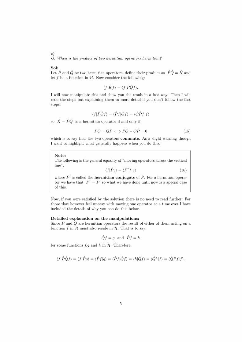
c)Q. When is the product of two hermitian operators hermitian?
Sol:Let P and Q be two hermitian operators, define their product as P Q = K andlet f be a function in H. Now consider the following:
〈f |Kf〉 = 〈f |P Qf〉.
I will now manipulate this and show you the result in a fast way. Then I willredo the steps but explaining them in more detail if you don’t follow the faststeps:
〈f |P Qf〉 = 〈P f |Qf〉 = 〈QP f |f〉
so K = P Q is a hermitian operator if and only if:
P Q = QP ⇐⇒ P Q− QP = 0 (15)
which is to say that the two operators commute. As a slight warning thoughI want to highlight what generally happens when you do this:
Note:The following is the general equality of ”moving operators across the verticalline”:
〈f |P g〉 = 〈P †f |g〉 (16)
where P † is called the hermitian conjugate of P . For a hermitian opera-tor we have that P † = P so what we have done until now is a special caseof this.
Now, if you were satisfied by the solution there is no need to read further. Forthose that however feel uneasy with moving one operator at a time over I haveincluded the details of why you can do this below.
Detailed explanation on the manipulations:Since P and Q are hermitian operators the result of either of them acting on afunction f in H must also reside in H. That is to say:
Qf = g and P f = h
for some functions f,g and h in H. Therefore:
〈f |P Qf〉 = 〈f |P g〉 = 〈P f |g〉 = 〈P f |Qf〉 = 〈h|Qf〉 = 〈Qh|f〉 = 〈QP f |f〉.
5
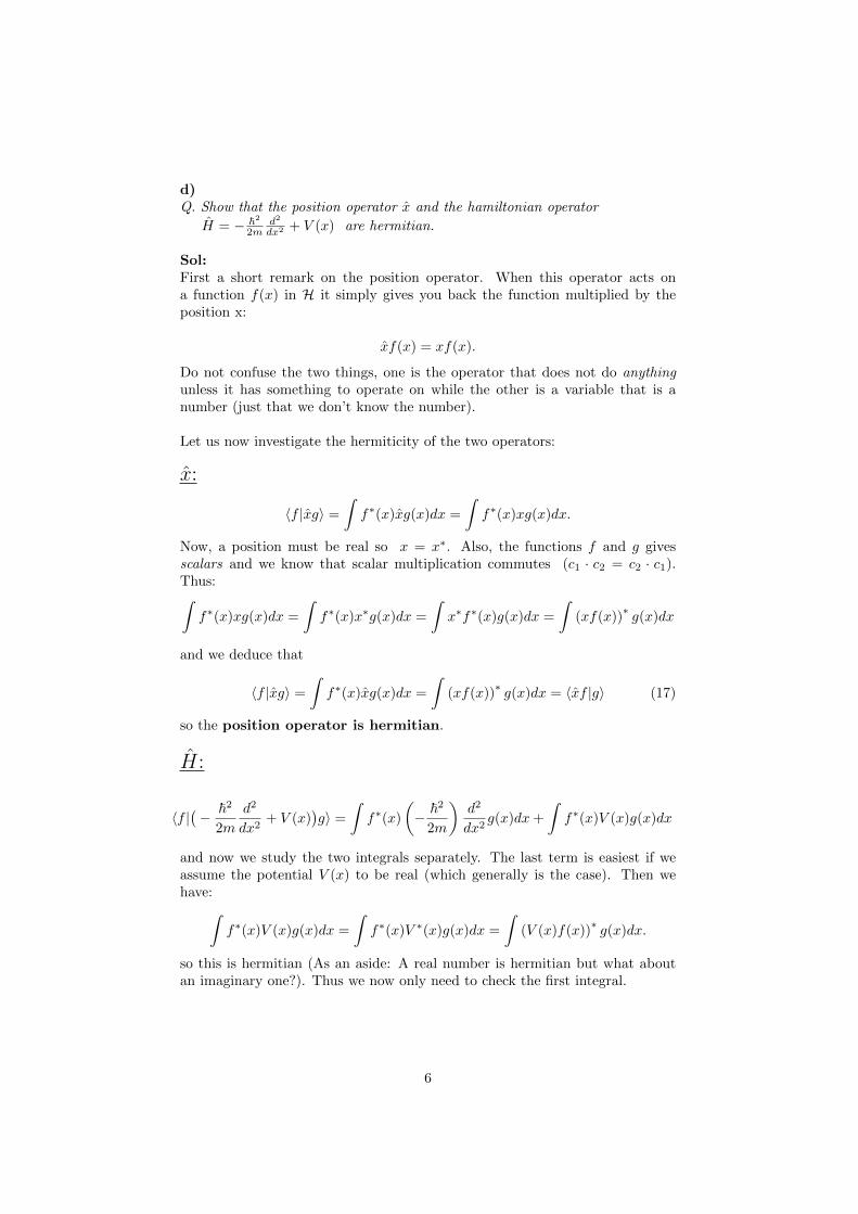
d)Q. Show that the position operator x and the hamiltonian operator
H = − ~2
2md2
dx2 + V (x) are hermitian.
Sol:First a short remark on the position operator. When this operator acts ona function f(x) in H it simply gives you back the function multiplied by theposition x:
xf(x) = xf(x).
Do not confuse the two things, one is the operator that does not do anythingunless it has something to operate on while the other is a variable that is anumber (just that we don’t know the number).
Let us now investigate the hermiticity of the two operators:
x:
〈f |xg〉 =
∫f∗(x)xg(x)dx =
∫f∗(x)xg(x)dx.
Now, a position must be real so x = x∗. Also, the functions f and g givesscalars and we know that scalar multiplication commutes (c1 · c2 = c2 · c1).Thus:∫f∗(x)xg(x)dx =
∫f∗(x)x∗g(x)dx =
∫x∗f∗(x)g(x)dx =
∫(xf(x))
∗g(x)dx
and we deduce that
〈f |xg〉 =
∫f∗(x)xg(x)dx =
∫(xf(x))
∗g(x)dx = 〈xf |g〉 (17)
so the position operator is hermitian.
H:
〈f |(− ~2
2m
d2
dx2+ V (x)
)g〉 =
∫f∗(x)
(− ~
2
2m
)d2
dx2g(x)dx+
∫f∗(x)V (x)g(x)dx
and now we study the two integrals separately. The last term is easiest if weassume the potential V (x) to be real (which generally is the case). Then wehave:∫
f∗(x)V (x)g(x)dx =
∫f∗(x)V ∗(x)g(x)dx =
∫(V (x)f(x))
∗g(x)dx.
so this is hermitian (As an aside: A real number is hermitian but what aboutan imaginary one?). Thus we now only need to check the first integral.
6
We can drop the real constant factor (why?) to get:
〈f | d2
dx2g〉 =
∫f∗d2g
dx2dx.
To compute this we need to know the limits of the integral which are ±∞ (sincenothing else is specified). Partial integration (twice) gives:
∫ ∞−∞
f∗d2g
dx2dx = f∗
dg
dx
∣∣∣∣∞−∞︸ ︷︷ ︸
0
−∫ ∞−∞
df∗
dx
dg
dxdx = − df∗
dxg
∣∣∣∣∞−∞︸ ︷︷ ︸
0
+
∫ ∞−∞
d2f∗
dx2gdx
where the underbraced terms are 0 because the the functions must go to 0 at±∞ and the derivatives are finite there2. Hence we have proven that:
〈f | d2
dx2g〉 = 〈 d
2
dx2f |g〉 (18)
so the hamiltonian operator is hermitian (since it is the sum of two her-mitian operators). Does this come as a surprise3?
3.5
The hermitian conjugate (or adjoint) of an operator Q is the operator Q†
such that:
〈f |Qg〉 = 〈Q†f |g〉 (19)
for all f and g in H. (For a hermitian operator then Q† = Q).
a)Q. Find the hermitian conjugates of x,i and d/dx.
Sol:Recall the following definition:
〈f |Qg〉 =
∫f∗(x)Qg(x)dx.
For the position operator we have (dropping notation of x-dependence):
〈f |xg〉 =
∫f∗xg dx =
∫f∗xg dx =
∫xf∗g dx =
∫(x∗f)
∗g dx. (20)
so for a variable (or constant) that represents a scalar the hermitian conjugateis the complex conjugation of that scalar. Because x is a real variable x = x∗
2This is the case for all physical functions at ±∞. When yo have finite limits on theintegral this need not be the case.
3Think about what the eigenvalues of H represent.
7
and we find that x† = x .
The imaginary number i is a scalar so from our discussion above we deduce
that i† = −i 4.
As goes for the derivative operator ddx (no need for a hat here either, we know
that it is an operator) we get:∫ ∞−∞
f∗d
dxg dx = f∗g
∣∣∣∣∞−∞︸ ︷︷ ︸
0
−∫ ∞−∞
df∗
dxg dx = −
∫ ∞−∞
df∗
dxg dx (21)
and we see that a
(d
dx
)†= − d
dx
b)Q. Construct the hermitian conjugate of the harmonic oscillator raising operatora+. Recall the definition of the step operators of the harmonic oscillator:
a+ =1√
2~mω(−ip+mωx) (22)
a− =1√
2~mω(ip+mωx) (23)
Sol:The hermitian conjugate of a sum of operators is the sum of the individualhermitian conjugates5. Thus we can study the two terms in a+ separately andwe notice that the second term is the position operator (multiplied by real con-stants). We know from the previous problem that this is a hermitian operatorso we now turn to study the first term: −ip.
Since momentum can be represented as p = ~iddx we see that
∓ ip = ∓ ~ ddx.
But we saw earlier that ∓ ddx = ±
(ddx
)†. Hence the hermitian conjugate of
−ip must be ip and we obtain:
(a+)† =1√
2~mω(ip+mωx) = a− (24)
4The hats on operators may be omitted if it from the context is clear that it is an operator.In this case writing i would be a waste of ink since a scalar acting as an operator is just a puremultiplication of that scalar. Furthermore it might be confused with the notation of basisvectors in a cartesian coordinate system.
5If this sounds strange you should pause a minute and explicitly write down the integralto convince yourself.
8
c)Show that (QR)† = R†Q†.
Sol:
We move one operator at a time:
〈f |QRg〉 = 〈Q†f |Rg〉 (25)
and as we do that we have to exchange the operator with its hermitian conjugate(recall problem 3.4c where we did this for hermitian operators). Now move theother operator:
〈Q†f |Rg〉 = 〈R†Q†f |g〉 (26)
so we have indeed proved that (QR)† = R†Q†
3.6
Q. Consider the operator Q = d2
dφ2 where φ is the azimuthal angle in polarcoordinates 0 ≤ φ ≤ 2π. The functions in H are subject to the conditionf(φ) = f(φ + 2π). Is Q hermitian? Find its eigenfunctions and eigenvalues.What is the spectrum? Is it degenerate?
Sol:Let f and g be functions in H defined on the interval (0, 2π). Now we check ifthe operator is hermitian:
〈f | d2
dφ2g〉 =
∫ 2π
0
f∗d2g
dφ2dφ = f∗
dg
dφ
∣∣∣∣2π0
−∫ 2π
0
df∗
dφ
dg
dφdφ.
The first term is 0 if you assume that the derivatives are continuous, whichamounts to the condition that functions are differentiable twice. For all systemswe will consider this can be assumed and we proceed with evaluating the lastintegral:
−∫ 2π
0
df∗
dφ
dg
dφdφ = − df∗
dφg
∣∣∣∣2π0︸ ︷︷ ︸
0
+
∫ 2π
0
d2f∗
dφ2g dφ.
Under the assumption that we made we have found that our operator is her-mitian. To find its eigenfunctions and eigenvalues we solve the eigenvalueequation:
Qf = qf
d2
dφ2f = qf =⇒ f = Ae
√qφ +Be−
√qφ (27)
9
The general solution is built up by a linear combination of the eigenfunctions:
f± = e±√qφ (28)
and q denotes our eigenvalues. Since any multiple of an eigenfunction is itselfan eigenfunction you could in principle multiply the exponential with a con-stant. However, this constant is accounted for when you normalize your linearcombination.
To see what the eigenvalues are we note that the boundary condition implies:
e±√qφ = e±
√q(φ+2π) =⇒ e±
√q2π = 1 = e2πin ∀n ∈ Z. (29)
This sets the condition on q:
q = −n2 ∀n ∈ Zq = 0,−1,−4,−9 . . .
which is called the spectrum of Q. For each value of q except 0 there aretwo distinct eigenfunctions, f+ and f−, so for q 6= 0 the spectrum is doublydegenerate. For q = 0 there is only one eigenfunction so for this eigenvalue itis not degenerate.
3.7
a)Q. Suppose that f(x) and g(x) are two eigenfunctions of an operator Q, withthe same eigenvalue q. Show that any linear combination of f and g is itself aneigenfunction of Q with the eigenvalue q.
Sol:This is very straightforward. We want to show that for any complex numbersc1, c2:
Q(c1f + c2g) = q(c1f + c2g)
holds if: Qf = qf and Qg = qg.
Since c1, c2 are just numbers, Q has no effect on them:
Q(c1f + c2g) = Qc1f + Qc2g = c1Qf + c2Qg
Now we use that Qf = qf and Qg = qg:
c1Qf + c2Qg = c1qf + c2qg = q(c1f + c2g)
so thus we have shown that:
Q(c1f + c2g) = q(c1f + c2g)
10
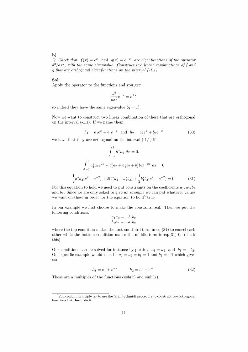
b)Q. Check that f(x) = ex and g(x) = e−x are eigenfunctions of the operatord2/dx2, with the same eigenvalue. Construct two linear combinations of f andg that are orthogonal eigenfunctions on the interval (-1,1).
Sol:Apply the operator to the functions and you get:
d2
dx2e±x = e±x
so indeed they have the same eigenvalue (q = 1).
Now we want to construct two linear combination of these that are orthogonalon the interval (-1,1). If we name them:
h1 = a1ex + b1e
−x and h2 = a2ex + b2e
−x (30)
we have that they are orthogonal on the interval (-1,1) if:∫ 1
−1h∗1h2 dx = 0.
∫ 1
−1a∗1a2e
2x + b∗1a2 + a∗1b2 + b∗1b2e−2x dx = 0
1
2a∗1a2(e2 − e−2) + 2(b∗1a2 + a∗1b2) +
1
2b∗1b2(e2 − e−2) = 0. (31)
For this equation to hold we need to put constraints on the coefficients a1, a2, b1and b2. Since we are only asked to give an example we can put whatever valueswe want on these in order for the equation to hold6 true.
In our example we first choose to make the constants real. Then we put thefollowing conditions:
a1a2 = −b1b2b1a2 = −a1b2
where the top condition makes the first and third term in eq.(31) to cancel eachother while the bottom condition makes the middle term in eq.(31) 0. (checkthis)
Our conditions can be solved for instance by putting a1 = a2 and b1 = −b2.One specific example would then be a1 = a2 = b1 = 1 and b2 = −1 which givesus:
h1 = ex + e−x h2 = ex − e−x (32)
These are a multiples of the functions cosh(x) and sinh(x).
6You could in principle try to use the Gram-Schmidt procedure to construct two orthogonalfunctions but don’t do it.
11
3.8
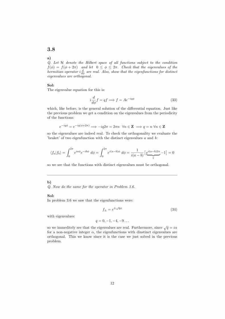
a)Q. Let H denote the Hilbert space of all functions subject to the conditionf(φ) = f(φ + 2π) and let 0 ≤ φ ≤ 2π. Check that the eigenvalues of thehermitian operator i ddφ are real. Also, show that the eigenfunctions for distincteigenvalues are orthogonal.
Sol:The eigenvalue equation for this is:
id
dφf = qf =⇒ f = Ae−iqφ (33)
which, like before, is the general solution of the differential equation. Just likethe previous problem we get a condition on the eigenvalues from the periodicityof the functions:
e−iqφ = e−iq(φ+2π) =⇒ −iq2π = 2πn ∀n ∈ Z =⇒ q = n ∀n ∈ Z
so the eigenvalues are indeed real. To check the orthogonality we evaluate the’braket’ of two eigenfunction with the distinct eigenvalues a and b:
〈fa|fb〉 =
∫ 2π
0
eiaφe−ibφ dφ =
∫ 2π
0
ei(a−b)φ dφ =1
i(a− b)[ei(a−b)2π︸ ︷︷ ︸
1
−1]
= 0
so we see that the functions with distinct eigenvalues must be orthogonal.
b)Q. Now do the same for the operator in Problem 3.6.
Sol:In problem 3.6 we saw that the eigenfunctions were:
f± = e±√qφ (34)
with eigenvalues:q = 0,−1,−4,−9 . . .
so we immeditely see that the eigenvalues are real. Furthermore, since√q = iα
for a non-negative integer α, the eigenfunctions with dinstinct eigenvalues areorthogonal. This we know since it is the case we just solved in the previousproblem.
12
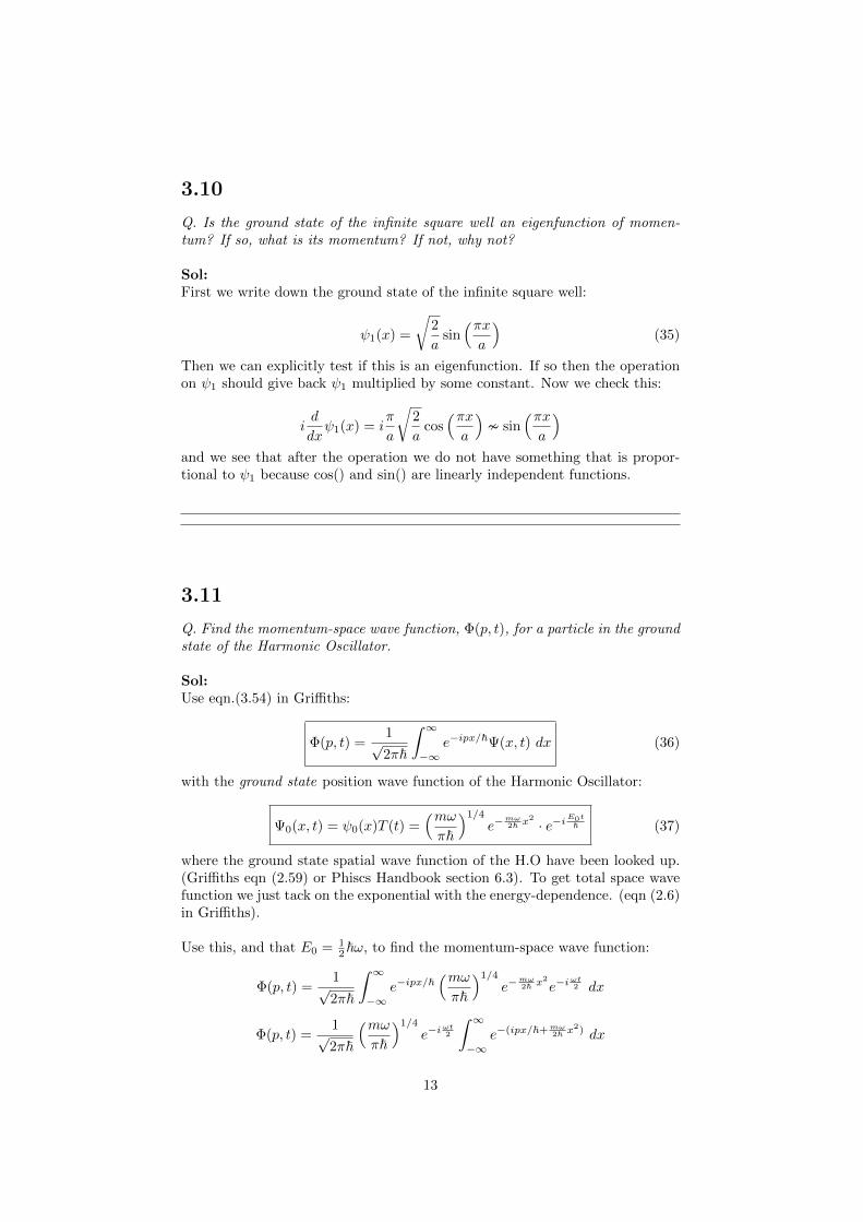
3.10
Q. Is the ground state of the infinite square well an eigenfunction of momen-tum? If so, what is its momentum? If not, why not?
Sol:First we write down the ground state of the infinite square well:
ψ1(x) =
√2
asin(πxa
)(35)
Then we can explicitly test if this is an eigenfunction. If so then the operationon ψ1 should give back ψ1 multiplied by some constant. Now we check this:
id
dxψ1(x) = i
π
a
√2
acos(πxa
)� sin
(πxa
)and we see that after the operation we do not have something that is propor-tional to ψ1 because cos() and sin() are linearly independent functions.
3.11
Q. Find the momentum-space wave function, Φ(p, t), for a particle in the groundstate of the Harmonic Oscillator.
Sol:Use eqn.(3.54) in Griffiths:
Φ(p, t) =1√2π~
∫ ∞−∞
e−ipx/~Ψ(x, t) dx (36)
with the ground state position wave function of the Harmonic Oscillator:
Ψ0(x, t) = ψ0(x)T (t) =(mωπ~
)1/4e−
mω2~ x
2
· e−iE0t~ (37)
where the ground state spatial wave function of the H.O have been looked up.(Griffiths eqn (2.59) or Phiscs Handbook section 6.3). To get total space wavefunction we just tack on the exponential with the energy-dependence. (eqn (2.6)in Griffiths).
Use this, and that E0 = 12~ω, to find the momentum-space wave function:
Φ(p, t) =1√2π~
∫ ∞−∞
e−ipx/~(mωπ~
)1/4e−
mω2~ x
2
e−iωt2 dx
Φ(p, t) =1√2π~
(mωπ~
)1/4e−i
ωt2
∫ ∞−∞
e−(ipx/~+mω2~ x
2) dx
13
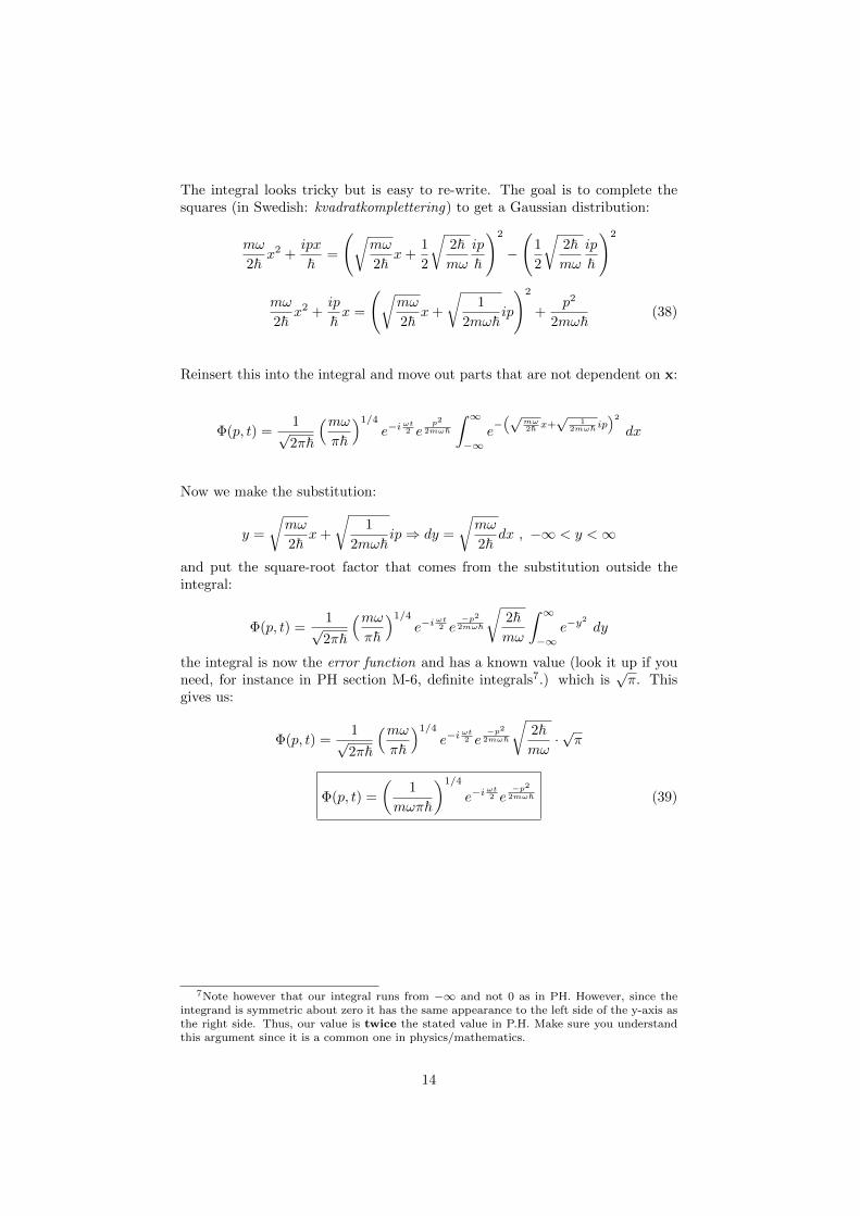
The integral looks tricky but is easy to re-write. The goal is to complete thesquares (in Swedish: kvadratkomplettering) to get a Gaussian distribution:
mω
2~x2 +
ipx
~=
(√mω
2~x+
1
2
√2~mω
ip
~
)2
−
(1
2
√2~mω
ip
~
)2
mω
2~x2 +
ip
~x =
(√mω
2~x+
√1
2mω~ip
)2
+p2
2mω~(38)
Reinsert this into the integral and move out parts that are not dependent on x:
Φ(p, t) =1√2π~
(mωπ~
)1/4e−i
ωt2 e
p2
2mω~
∫ ∞−∞
e−(√
mω2~ x+
√1
2mω~ ip)2
dx
Now we make the substitution:
y =
√mω
2~x+
√1
2mω~ip⇒ dy =
√mω
2~dx , −∞ < y <∞
and put the square-root factor that comes from the substitution outside theintegral:
Φ(p, t) =1√2π~
(mωπ~
)1/4e−i
ωt2 e
−p2
2mω~
√2~mω
∫ ∞−∞
e−y2
dy
the integral is now the error function and has a known value (look it up if youneed, for instance in PH section M-6, definite integrals7.) which is
√π. This
gives us:
Φ(p, t) =1√2π~
(mωπ~
)1/4e−i
ωt2 e
−p2
2mω~
√2~mω·√π
Φ(p, t) =
(1
mωπ~
)1/4
e−iωt2 e
−p2
2mω~ (39)
7Note however that our integral runs from −∞ and not 0 as in PH. However, since theintegrand is symmetric about zero it has the same appearance to the left side of the y-axis asthe right side. Thus, our value is twice the stated value in P.H. Make sure you understandthis argument since it is a common one in physics/mathematics.
14
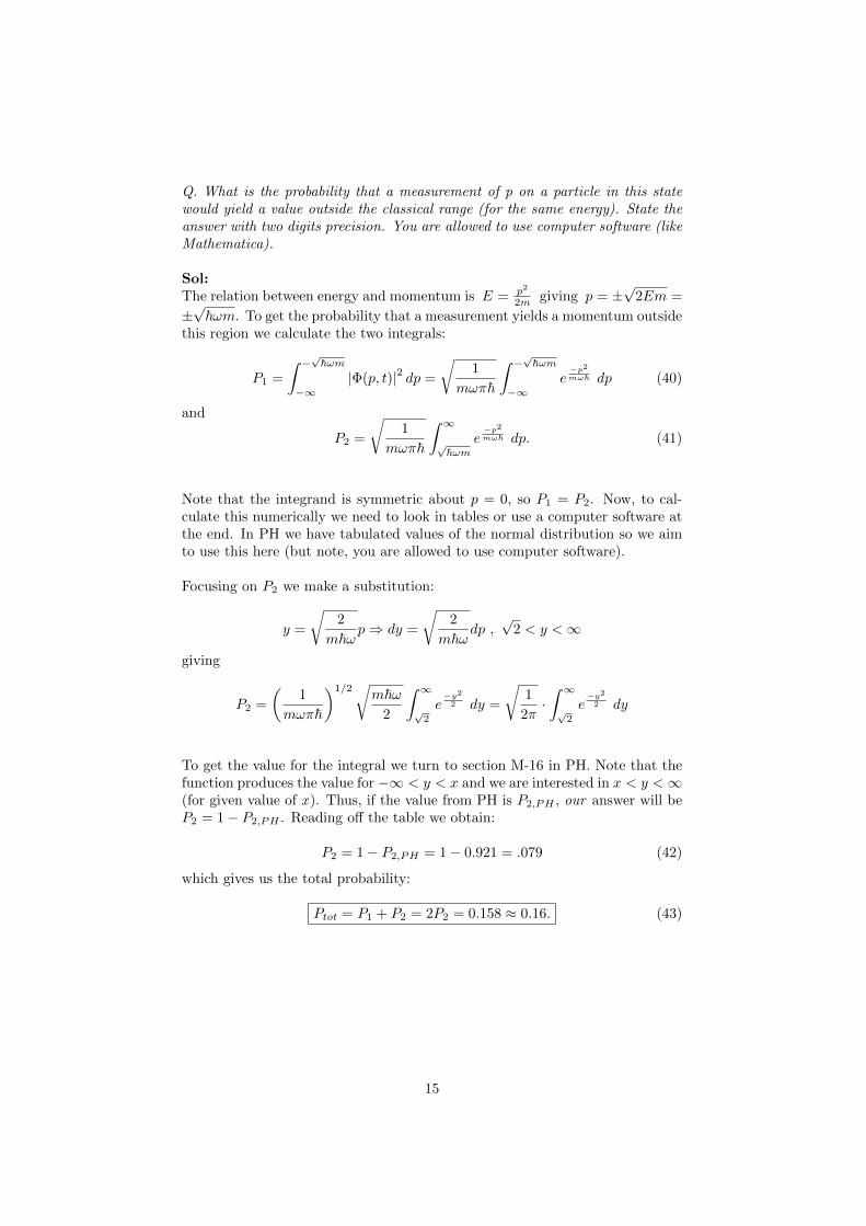
Q. What is the probability that a measurement of p on a particle in this statewould yield a value outside the classical range (for the same energy). State theanswer with two digits precision. You are allowed to use computer software (likeMathematica).
Sol:The relation between energy and momentum is E = p2
2m giving p = ±√
2Em =
±√~ωm. To get the probability that a measurement yields a momentum outside
this region we calculate the two integrals:
P1 =
∫ −√~ωm
−∞|Φ(p, t)|2 dp =
√1
mωπ~
∫ −√~ωm
−∞e−p2
mω~ dp (40)
and
P2 =
√1
mωπ~
∫ ∞√~ωm
e−p2
mω~ dp. (41)
Note that the integrand is symmetric about p = 0, so P1 = P2. Now, to cal-culate this numerically we need to look in tables or use a computer software atthe end. In PH we have tabulated values of the normal distribution so we aimto use this here (but note, you are allowed to use computer software).
Focusing on P2 we make a substitution:
y =
√2
m~ωp⇒ dy =
√2
m~ωdp ,
√2 < y <∞
giving
P2 =
(1
mωπ~
)1/2√m~ω
2
∫ ∞√2
e−y2
2 dy =
√1
2π·∫ ∞√2
e−y2
2 dy
To get the value for the integral we turn to section M-16 in PH. Note that thefunction produces the value for −∞ < y < x and we are interested in x < y <∞(for given value of x ). Thus, if the value from PH is P2,PH , our answer will beP2 = 1− P2,PH . Reading off the table we obtain:
P2 = 1− P2,PH = 1− 0.921 = .079 (42)
which gives us the total probability:
Ptot = P1 + P2 = 2P2 = 0.158 ≈ 0.16. (43)
15
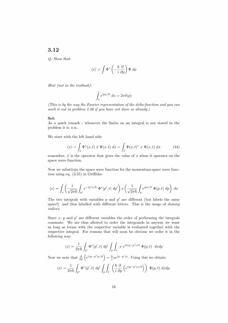
3.12
Q. Show that:
〈x〉 =
∫Φ∗(−~i
∂
∂p
)Φ dp
Hint (not in the textbook): ∫x
eipx/~ dx = 2πδ(p)
(This is by the way the Fourier representation of the delta-function and you canwork it out in problem 2.26 if you have not done so already.)
Sol:As a quick remark - whenever the limits on an integral is not stated in theproblem it is ±∞.
We start with the left hand side:
〈x〉 =
∫x
Ψ∗(x, t) x Ψ(x, t) dx =
∫x
Ψ(x, t)∗ x Ψ(x, t) dx (44)
remember, x is the operator that gives the value of x when it operates on thespace wave function.
Now we substitute the space wave function for the momentum-space wave func-tion using eq. (3.55) in Griffiths:
〈x〉 =
∫x
(1√2π~
∫p′e−ip
′x/~ Φ∗(p′, t) dp′)x
(1√2π~
∫p
eipx/~ Φ(p, t) dp
)dx
The two integrals with variables p and p′ are different (but labels the samespace!) and thus labelled with different letters. This is the usage of dummyindices.
Since x, p and p′ are different variables the order of performing the integralscommute. We are thus allowed to order the integrands in anyway we wantas long as terms with the respective variable is evaluated together with therespective integral. For reasons that will soon be obvious we order it in thefollowing way:
〈x〉 =1
2π~
∫p′
Φ∗(p′, t) dp′∫p
∫x
x eix(p−p′)/~ Φ(p, t) dxdp
Now we note that ∂∂p
(ei(p−p
′)x/~)
= ~i xe
(p−p′)x. Using this we obtain:
〈x〉 =1
2π~
∫p′
Φ∗(p′, t) dp′∫p
∫x
(~i
∂
∂p
(ei(p−p
′)x/~))
Φ(p, t) dxdp.
16
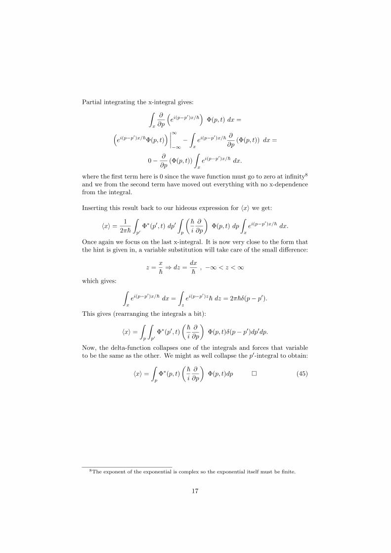
Partial integrating the x-integral gives:∫x
∂
∂p
(ei(p−p
′)x/~)
Φ(p, t) dx =
(ei(p−p
′)x/~Φ(p, t)) ∣∣∣∣∞−∞−∫x
ei(p−p′)x/~ ∂
∂p(Φ(p, t)) dx =
0− ∂
∂p(Φ(p, t))
∫x
ei(p−p′)x/~ dx.
where the first term here is 0 since the wave function must go to zero at infinity8
and we from the second term have moved out everything with no x-dependencefrom the integral.
Inserting this result back to our hideous expression for 〈x〉 we get:
〈x〉 =1
2π~
∫p′
Φ∗(p′, t) dp′∫p
(~i
∂
∂p
)Φ(p, t) dp
∫x
ei(p−p′)x/~ dx.
Once again we focus on the last x-integral. It is now very close to the form thatthe hint is given in, a variable substitution will take care of the small difference:
z =x
~⇒ dz =
dx
~, −∞ < z <∞
which gives: ∫x
ei(p−p′)x/~ dx =
∫z
ei(p−p′)z~ dz = 2π~δ(p− p′).
This gives (rearranging the integrals a bit):
〈x〉 =
∫p
∫p′
Φ∗(p′, t)
(~i
∂
∂p
)Φ(p, t)δ(p− p′)dp′dp.
Now, the delta-function collapses one of the integrals and forces that variableto be the same as the other. We might as well collapse the p′-integral to obtain:
〈x〉 =
∫p
Φ∗(p, t)
(~i
∂
∂p
)Φ(p, t)dp � (45)
8The exponent of the exponential is complex so the exponential itself must be finite.
17
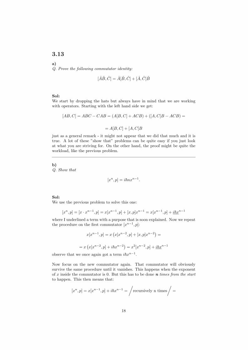
3.13
a)Q. Prove the following commutator identity:
[AB, C] = A[B, C] + [A, C]B
Sol:We start by dropping the hats but always have in mind that we are workingwith operators. Starting with the left hand side we get:
[AB,C] = ABC − CAB = (A[B,C] +ACB) + ([A,C]B −ACB) =
= A[B,C] + [A,C]B
just as a general remark - it might not appear that we did that much and it istrue. A lot of these ”show that” problems can be quite easy if you just lookat what you are striving for. On the other hand, the proof might be quite theworkload, like the previous problem.
b)Q. Show that
[xn, p] = i~nxn−1.
Sol:We use the previous problem to solve this one:
[xn, p] = [x · xn−1, p] = x[xn−1, p] + [x, p]xn−1 = x[xn−1, p] + i~xn−1
where I underlined a term with a purpose that is soon explained. Now we repeatthe procedure on the first commutator [xn−1, p]:
x[xn−1, p] = x(x[xn−2, p] + [x, p]xn−2
)=
= x(x[xn−2, p] + i~xn−2
)= x2[xn−2, p] + i~xn−1
observe that we once again got a term i~xn−1.
Now focus on the new commutator again. That commutator will obviouslysurvive the same procedure until it vanishes. This happens when the exponentof x inside the commutator is 0. But this has to be done n times from the startto happen. This then means that:
[xn, p] = x[xn−1, p] + i~xn−1 =
/recursively n times
/=
18
0 + i~xn−1 + . . .+ i~xn−1︸ ︷︷ ︸n elements
= i~nxn−1. �
c)Q. Show more generally that
[f(x), p] = i~df
dx
for any function f(x).
Sol:Here we will need to use the explicit form of the momentum operator. Wheneveryou use the explicit form it is best to have a test function to work with, otherwiseyou probably will do something crazy. Let g(x) be such a test function.
[f(x), p]g(x) = f(x)pg(x)−pf(x)g(x) = f(x)
(~i
d
dx
)g(x)−
(~i
d
dx
)f(x)g(x) =
~i
[f(x)
dg
dx−(df
dxg(x) +
dg
dxf(x)
)]= −~
i
df
dxg(x)
Now that the test function has fulfilled its purpose we can throw it away toconclude:
[f(x), p] = i~df
dx. (46)
3.14
Q. Prove the famous ”(your name) uncertainty principle”, relating the uncer-tainty in position (A = x) to the uncertainty in energy H = p2/2m+ V :
σxσH ≥~
2m|〈p〉|
For stationary states this doesn’t tell you much - why not?
Sol:In section 3.5 in the textbook Griffiths derives the generalized uncertainty prin-ciple:
σ2Aσ
2B ≥
(1
2i〈[A, B]〉
)2
(47)
19
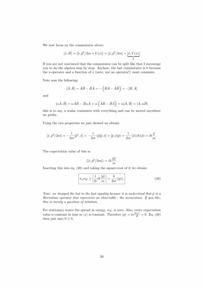
We now focus on the commutator above:
[x, H] = [x, p2/2m+ V (x)] = [x, p2/2m] + [x, V (x)]︸ ︷︷ ︸0
If you are not convinced that the commutator can be split like that I encourageyou to do the algebra step by step. Anyhow, the last commutator is 0 becausethe x-operator and a function of x (note, not an operator!) must commute.
Note now the following:
[A, B] = AB − BA = −(BA− AB
)= −[B, A]
and
[αA, B] = αAB − BαA = α(AB − BA
)= α[A, B] = [A, αB]
this is to say, a scalar commutes with everything and can be moved anywherewe prefer.
Using the two properties we just showed we obtain:
[x, p2/2m] = − 1
2m[p2, x] = − 1
2m(p[p, x] + [p, x]p) =
1
2m(2 (i~) p) = i~
p
m.
The expectation value of this is:
〈[x, p2/2m]〉 = i~〈p〉m.
Inserting this into eq. (48) and taking the square-root of it we obtain:
σxσH ≥∣∣∣∣ 1
2ii~〈p〉m
∣∣∣∣ =~
2m|〈p〉|. (48)
Note: we dropped the hat in the last equality because it is understood that p is aHermitian operator that represents an observable - the momentum. If you like,this is merely a question of notation.
For stationary states the spread in energy, σH , is zero. Also, every expectation
value is constant in time so 〈x〉 is constant. Therefore 〈p〉 = md〈x〉dt = 0. Eq. (48)
then just says 0 ≥ 0.
20
3.15
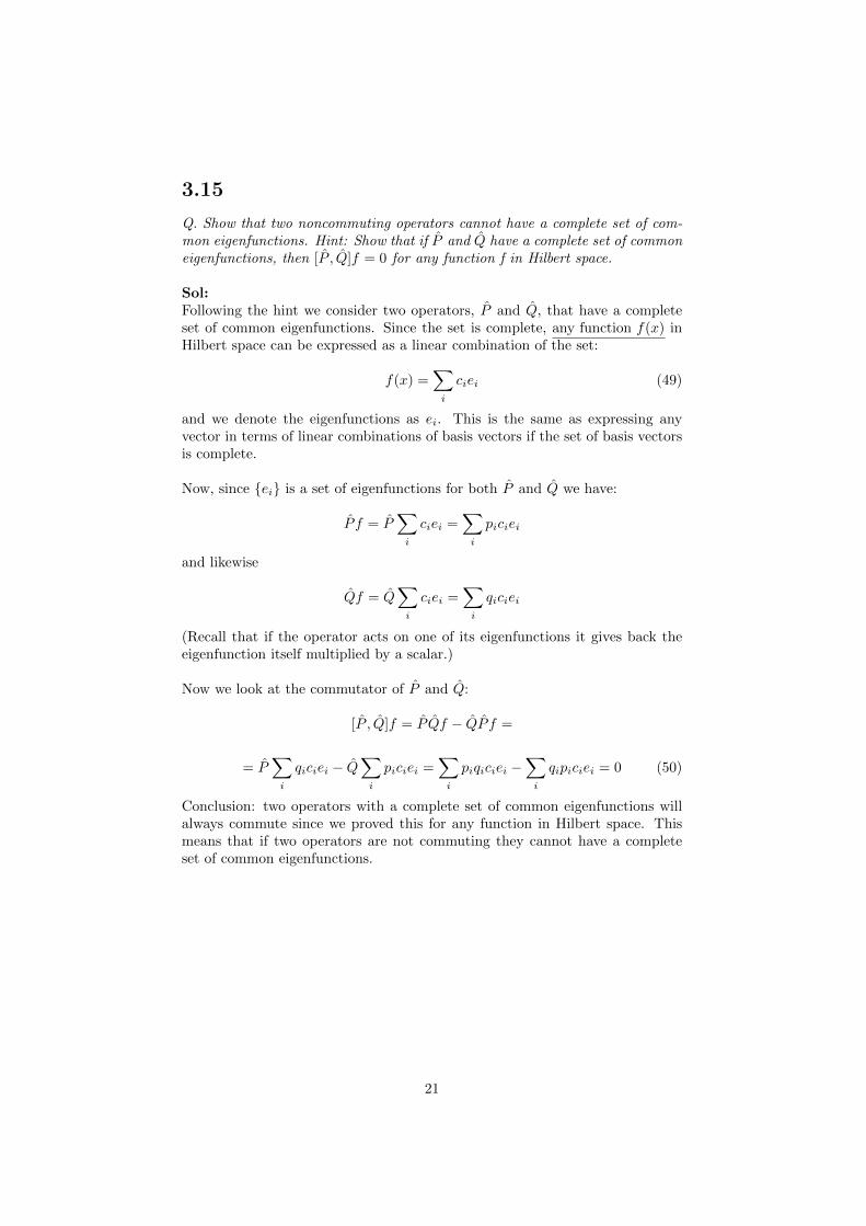
Q. Show that two noncommuting operators cannot have a complete set of com-mon eigenfunctions. Hint: Show that if P and Q have a complete set of commoneigenfunctions, then [P , Q]f = 0 for any function f in Hilbert space.
Sol:Following the hint we consider two operators, P and Q, that have a completeset of common eigenfunctions. Since the set is complete, any function f(x) inHilbert space can be expressed as a linear combination of the set:
f(x) =∑i
ciei (49)
and we denote the eigenfunctions as ei. This is the same as expressing anyvector in terms of linear combinations of basis vectors if the set of basis vectorsis complete.
Now, since {ei} is a set of eigenfunctions for both P and Q we have:
P f = P∑i
ciei =∑i
piciei
and likewise
Qf = Q∑i
ciei =∑i
qiciei
(Recall that if the operator acts on one of its eigenfunctions it gives back theeigenfunction itself multiplied by a scalar.)
Now we look at the commutator of P and Q:
[P , Q]f = P Qf − QP f =
= P∑i
qiciei − Q∑i
piciei =∑i
piqiciei −∑i
qipiciei = 0 (50)
Conclusion: two operators with a complete set of common eigenfunctions willalways commute since we proved this for any function in Hilbert space. Thismeans that if two operators are not commuting they cannot have a completeset of common eigenfunctions.
21
3.16
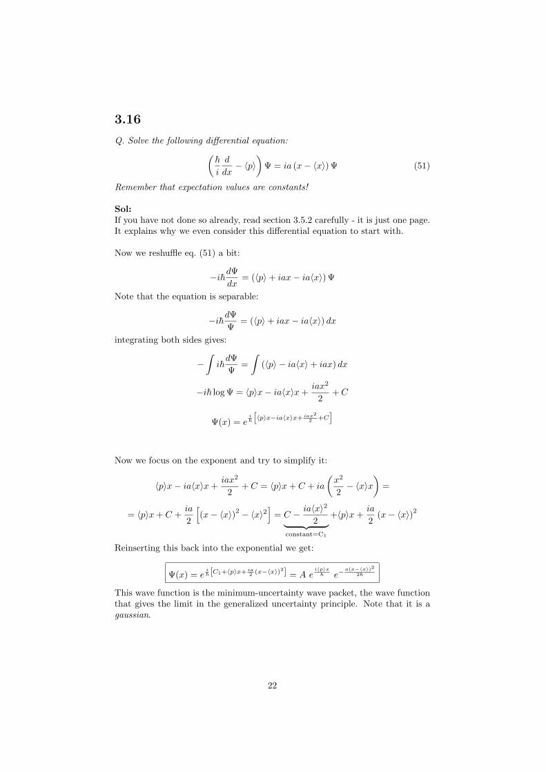
Q. Solve the following differential equation:(~i
d
dx− 〈p〉
)Ψ = ia (x− 〈x〉) Ψ (51)
Remember that expectation values are constants!
Sol:If you have not done so already, read section 3.5.2 carefully - it is just one page.It explains why we even consider this differential equation to start with.
Now we reshuffle eq. (51) a bit:
−i~dΨ
dx= (〈p〉+ iax− ia〈x〉) Ψ
Note that the equation is separable:
−i~dΨ
Ψ= (〈p〉+ iax− ia〈x〉) dx
integrating both sides gives:
−∫i~dΨ
Ψ=
∫(〈p〉 − ia〈x〉+ iax) dx
−i~ log Ψ = 〈p〉x− ia〈x〉x+iax2
2+ C
Ψ(x) = ei~
[〈p〉x−ia〈x〉x+ iax2
2 +C]
Now we focus on the exponent and try to simplify it:
〈p〉x− ia〈x〉x+iax2
2+ C = 〈p〉x+ C + ia
(x2
2− 〈x〉x
)=
= 〈p〉x+ C +ia
2
[(x− 〈x〉)2 − 〈x〉2
]= C − ia〈x〉2
2︸ ︷︷ ︸constant=C1
+〈p〉x+ia
2(x− 〈x〉)2
Reinserting this back into the exponential we get:
Ψ(x) = ei~ [C1+〈p〉x+ ia
2 (x−〈x〉)2] = A ei〈p〉x
~ e−a(x−〈x〉)2
2~
This wave function is the minimum-uncertainty wave packet, the wave functionthat gives the limit in the generalized uncertainty principle. Note that it is agaussian.
22
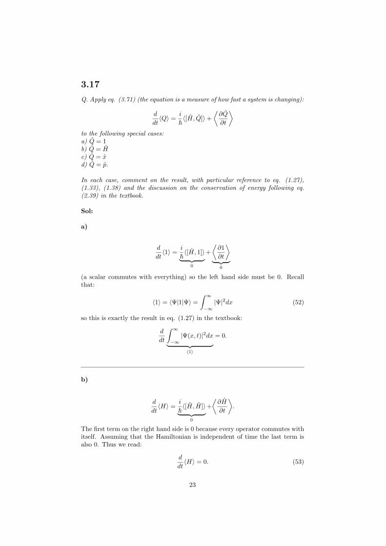
3.17
Q. Apply eq. (3.71) (the equation is a measure of how fast a system is changing):
d
dt〈Q〉 =
i
~〈[H, Q]〉+
⟨∂Q
∂t
⟩to the following special cases:a) Q = 1b) Q = Hc) Q = xd) Q = p.
In each case, comment on the result, with particular reference to eq. (1.27),(1.33), (1.38) and the discussion on the conservation of energy following eq.(2.39) in the textbook.
Sol:
a)
d
dt〈1〉 =
i
~〈[H, 1]〉︸ ︷︷ ︸
0
+
⟨∂1
∂t
⟩︸ ︷︷ ︸
0
(a scalar commutes with everything) so the left hand side must be 0. Recallthat:
〈1〉 = 〈Ψ|1|Ψ〉 =
∫ ∞−∞|Ψ|2dx (52)
so this is exactly the result in eq. (1.27) in the textbook:
d
dt
∫ ∞−∞|Ψ(x, t)|2dx︸ ︷︷ ︸〈1〉
= 0.
b)
d
dt〈H〉 =
i
~〈[H, H]〉︸ ︷︷ ︸
0
+
⟨∂H
∂t
⟩.
The first term on the right hand side is 0 because every operator commutes withitself. Assuming that the Hamiltonian is independent of time the last term isalso 0. Thus we read:
d
dt〈H〉 = 0. (53)
23
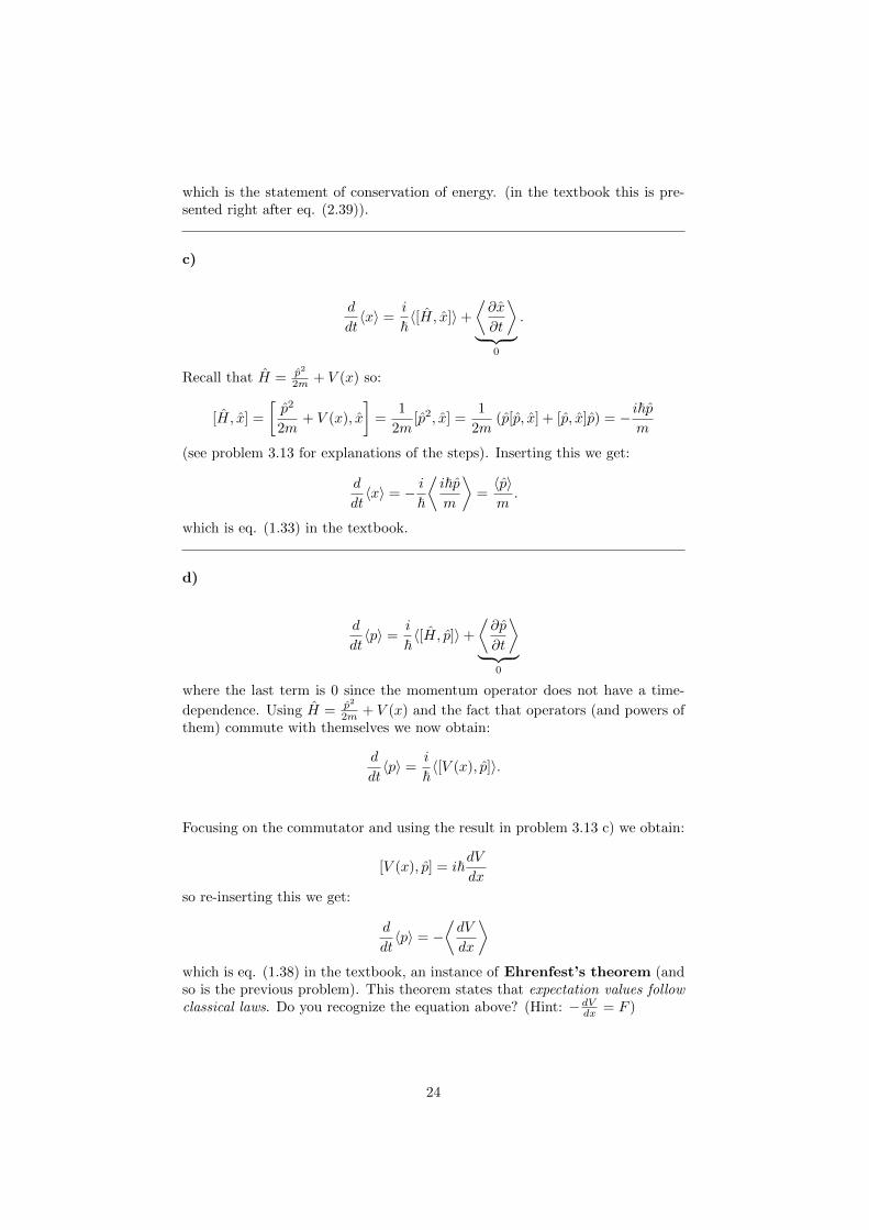
which is the statement of conservation of energy. (in the textbook this is pre-sented right after eq. (2.39)).
c)
d
dt〈x〉 =
i
~〈[H, x]〉+
⟨∂x
∂t
⟩︸ ︷︷ ︸
0
.
Recall that H = p2
2m + V (x) so:
[H, x] =
[p2
2m+ V (x), x
]=
1
2m[p2, x] =
1
2m(p[p, x] + [p, x]p) = − i~p
m
(see problem 3.13 for explanations of the steps). Inserting this we get:
d
dt〈x〉 = − i
~
⟨i~pm
⟩=〈p〉m.
which is eq. (1.33) in the textbook.
d)
d
dt〈p〉 =
i
~〈[H, p]〉+
⟨∂p
∂t
⟩︸ ︷︷ ︸
0
where the last term is 0 since the momentum operator does not have a time-
dependence. Using H = p2
2m + V (x) and the fact that operators (and powers ofthem) commute with themselves we now obtain:
d
dt〈p〉 =
i
~〈[V (x), p]〉.
Focusing on the commutator and using the result in problem 3.13 c) we obtain:
[V (x), p] = i~dV
dx
so re-inserting this we get:
d
dt〈p〉 = −
⟨dV
dx
⟩which is eq. (1.38) in the textbook, an instance of Ehrenfest’s theorem (andso is the previous problem). This theorem states that expectation values followclassical laws. Do you recognize the equation above? (Hint: −dVdx = F )
24
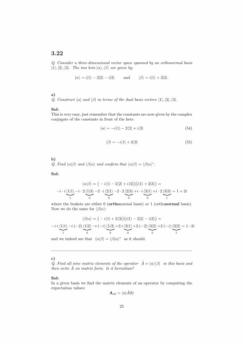
3.22
Q. Consider a three-dimensional vector space spanned by an orthonormal basis|1〉, |2〉, |3〉. The two kets |α〉, |β〉 are given by:
|α〉 = i|1〉 − 2|2〉 − i|3〉 and |β〉 = i|1〉+ 2|3〉.
a)Q. Construct 〈α| and 〈β| in terms of the dual basis vectors 〈1|, 〈2|, 〈3|.
Sol:This is very easy, just remember that the constants are now given by the complexconjugate of the constants in front of the kets:
〈α| = −i〈1| − 2〈2|+ i〈3| (54)
〈β| = −i〈1|+ 2〈3| (55)
b)Q. Find 〈α|β〉 and 〈β|α〉 and confirm that 〈α|β〉 = 〈β|α〉∗.
Sol:
〈α|β〉 =(− i〈1| − 2〈2|+ i〈3|
)(i|1〉+ 2|3〉
)=
−i · i 〈1|1〉︸︷︷︸1
−i · 2 〈1|3〉︸︷︷︸0
−2 · i 〈2|1〉︸︷︷︸0
−2 · 2 〈2|3〉︸︷︷︸0
+i · i 〈3|1〉︸︷︷︸0
+i · 2 〈3|3〉︸︷︷︸1
= 1 + 2i
where the brakets are either 0 (orthonormal basis) or 1 (orthonormal basis).Now we do the same for 〈β|α〉:
〈β|α〉 =(− i〈1|+ 2〈3|
)(i|1〉 − 2|2〉 − i|3〉
)=
−i·i 〈1|1〉︸︷︷︸1
−i·(−2) 〈1|2〉︸︷︷︸0
−i·(−i) 〈1|3〉︸︷︷︸0
+2·i 〈3|1〉︸︷︷︸0
+2·(−2) 〈3|2〉︸︷︷︸0
+2·(−i) 〈3|3〉︸︷︷︸1
= 1−2i
and we indeed see that 〈α|β〉 = 〈β|α〉∗ as it should.
c)Q. Find all nine matrix elements of the operator A = |α〉〈β| in this basis andthen write A on matrix form. Is it hermitian?
Sol:In a given basis we find the matrix elements of an operator by computing theexpectation values:
Aab = 〈a|A|b〉
25
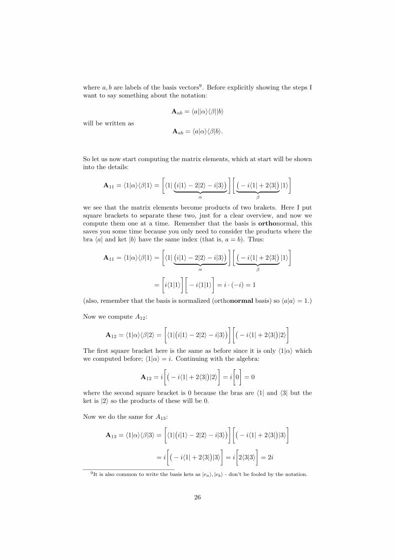
where a, b are labels of the basis vectors9. Before explicitly showing the steps Iwant to say something about the notation:
Aab = 〈a||α〉〈β||b〉
will be written asAab = 〈a|α〉〈β|b〉.
So let us now start computing the matrix elements, which at start will be showninto the details:
A11 = 〈1|α〉〈β|1〉 =
[〈1|(i|1〉 − 2|2〉 − i|3〉
)︸ ︷︷ ︸α
][ (− i〈1|+ 2〈3|
)︸ ︷︷ ︸β
|1〉]
we see that the matrix elements become products of two brakets. Here I putsquare brackets to separate these two, just for a clear overview, and now wecompute them one at a time. Remember that the basis is orthonormal, thissaves you some time because you only need to consider the products where thebra 〈a| and ket |b〉 have the same index (that is, a = b). Thus:
A11 = 〈1|α〉〈β|1〉 =
[〈1|(i|1〉 − 2|2〉 − i|3〉
)︸ ︷︷ ︸α
][ (− i〈1|+ 2〈3|
)︸ ︷︷ ︸β
|1〉]
=
[i〈1|1〉
][− i〈1|1〉
]= i · (−i) = 1
(also, remember that the basis is normalized (orthonormal basis) so 〈a|a〉 = 1.)
Now we compute A12:
A12 = 〈1|α〉〈β|2〉 =
[〈1|(i|1〉 − 2|2〉 − i|3〉
)][(− i〈1|+ 2〈3|
)|2〉]
The first square bracket here is the same as before since it is only 〈1|α〉 whichwe computed before; 〈1|α〉 = i. Continuing with the algebra:
A12 = i
[(− i〈1|+ 2〈3|
)|2〉]
= i
[0
]= 0
where the second square bracket is 0 because the bras are 〈1| and 〈3| but theket is |2〉 so the products of these will be 0.
Now we do the same for A13:
A13 = 〈1|α〉〈β|3〉 =
[〈1|(i|1〉 − 2|2〉 − i|3〉
)][(− i〈1|+ 2〈3|
)|3〉]
= i
[(− i〈1|+ 2〈3|
)|3〉]
= i
[2〈3|3〉
]= 2i
9It is also common to write the basis kets as |ea〉, |eb〉 - don’t be fooled by the notation.
26
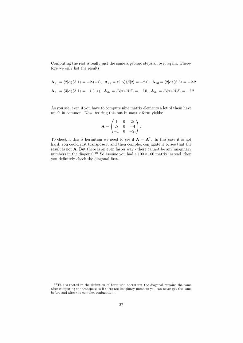
Computing the rest is really just the same algebraic steps all over again. There-fore we only list the results:
A21 = 〈2|α〉〈β|1〉 = −2·(−i), A22 = 〈2|α〉〈β|2〉 = −2·0, A23 = 〈2|α〉〈β|3〉 = −2·2
A31 = 〈3|α〉〈β|1〉 = −i·(−i), A32 = 〈3|α〉〈β|2〉 = −i·0, A33 = 〈3|α〉〈β|3〉 = −i·2
As you see, even if you have to compute nine matrix elements a lot of them havemuch in common. Now, writing this out in matrix form yields:
A =
1 0 2i2i 0 −4−1 0 −2i
.
To check if this is hermitian we need to see if A = A†. In this case it is nothard, you could just transpose it and then complex conjugate it to see that theresult is not A. But there is an even faster way - there cannot be any imaginarynumbers in the diagonal!10 So assume you had a 100×100 matrix instead, thenyou definitely check the diagonal first.
10This is rooted in the definition of hermitian operators: the diagonal remains the sameafter computing the transpose so if there are imaginary numbers you can never get the samebefore and after the complex conjugation.
27
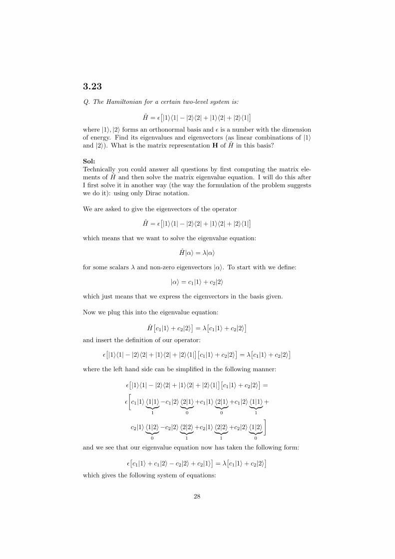
3.23
Q. The Hamiltonian for a certain two-level system is:
H = ε[|1〉〈1| − |2〉〈2|+ |1〉〈2|+ |2〉〈1|
]where |1〉, |2〉 forms an orthonormal basis and ε is a number with the dimensionof energy. Find its eigenvalues and eigenvectors (as linear combinations of |1〉and |2〉). What is the matrix representation H of H in this basis?
Sol:Technically you could answer all questions by first computing the matrix ele-ments of H and then solve the matrix eigenvalue equation. I will do this afterI first solve it in another way (the way the formulation of the problem suggestswe do it): using only Dirac notation.
We are asked to give the eigenvectors of the operator
H = ε[|1〉〈1| − |2〉〈2|+ |1〉〈2|+ |2〉〈1|
]which means that we want to solve the eigenvalue equation:
H|α〉 = λ|α〉
for some scalars λ and non-zero eigenvectors |α〉. To start with we define:
|α〉 = c1|1〉+ c2|2〉
which just means that we express the eigenvectors in the basis given.
Now we plug this into the eigenvalue equation:
H[c1|1〉+ c2|2〉
]= λ
[c1|1〉+ c2|2〉
]and insert the definition of our operator:
ε[|1〉〈1| − |2〉〈2|+ |1〉〈2|+ |2〉〈1|
][c1|1〉+ c2|2〉
]= λ
[c1|1〉+ c2|2〉
]where the left hand side can be simplified in the following manner:
ε[|1〉〈1| − |2〉〈2|+ |1〉〈2|+ |2〉〈1|
][c1|1〉+ c2|2〉
]=
ε
[c1|1〉 〈1|1〉︸︷︷︸
1
−c1|2〉 〈2|1〉︸︷︷︸0
+c1|1〉 〈2|1〉︸︷︷︸0
+c1|2〉 〈1|1〉︸︷︷︸1
+
c2|1〉 〈1|2〉︸︷︷︸0
−c2|2〉 〈2|2〉︸︷︷︸1
+c2|1〉 〈2|2〉︸︷︷︸1
+c2|2〉 〈1|2〉︸︷︷︸0
]and we see that our eigenvalue equation now has taken the following form:
ε[c1|1〉+ c1|2〉 − c2|2〉+ c2|1〉
]= λ
[c1|1〉+ c2|2〉
]which gives the following system of equations:
28
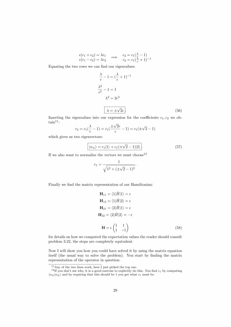
ε(c1 + c2) = λc1ε(c1 − c2) = λc2
=⇒ c2 = c1(λε − 1)c2 = c1(λε + 1)−1
Equating the two rows we can find our eigenvalues:
λ
ε− 1 = (
λ
ε+ 1)−1
λ2
ε2− 1 = 1
λ2 = 2ε2
λ = ±√
2ε . (56)
Inserting the eigenvalues into our expression for the coefficients c1, c2 we ob-tain11:
c2 = c1(λ
ε− 1) = c1(
±√
2ε
ε− 1) = c1(±
√2− 1)
which gives us two eigenvectors:
|α±〉 = c1|1〉+ c1(±√
2− 1)|2〉 . (57)
If we also want to normalize the vectors we must choose12
c1 =1√
12 + (±√
2− 1)2.
Finally we find the matrix representation of our Hamiltonian:
H11 = 〈1|H|1〉 = ε
H12 = 〈1|H|2〉 = ε
H21 = 〈2|H|1〉 = ε
H22 = 〈2|H|2〉 = −ε
H = ε
(1 11 −1
)(58)
for details on how we computed the expectation values the reader should consultproblem 3.22, the steps are completely equivalent.
Now I will show you how you could have solved it by using the matrix equationitself (the usual way to solve the problem). You start by finding the matrixrepresentation of the operator in question:
11Any of the two lines work, here I just picked the top one.12If you don’t see why, it is a good exercise to explicitly do this. You find c1 by computing〈α±|α±〉 and by requiring that this should be 1 you get what c1 must be.
29
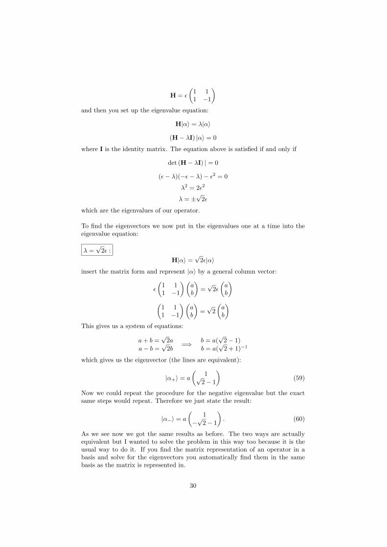
H = ε
(1 11 −1
)and then you set up the eigenvalue equation:
H|α〉 = λ|α〉
(H− λI) |α〉 = 0
where I is the identity matrix. The equation above is satisfied if and only if
det (H− λI) | = 0
(ε− λ)(−ε− λ)− ε2 = 0
λ2 = 2ε2
λ = ±√
2ε
which are the eigenvalues of our operator.
To find the eigenvectors we now put in the eigenvalues one at a time into theeigenvalue equation:
λ =√
2ε :
H|α〉 =√
2ε|α〉
insert the matrix form and represent |α〉 by a general column vector:
ε
(1 11 −1
)(ab
)=√
2ε
(ab
)(
1 11 −1
)(ab
)=√
2
(ab
)This gives us a system of equations:
a+ b =√
2a
a− b =√
2b=⇒ b = a(
√2− 1)
b = a(√
2 + 1)−1
which gives us the eigenvector (the lines are equivalent):
|α+〉 = a
(1√
2− 1
)(59)
Now we could repeat the procedure for the negative eigenvalue but the exactsame steps would repeat. Therefore we just state the result:
|α−〉 = a
(1
−√
2− 1
). (60)
As we see now we got the same results as before. The two ways are actuallyequivalent but I wanted to solve the problem in this way too because it is theusual way to do it. If you find the matrix representation of an operator in abasis and solve for the eigenvectors you automatically find them in the samebasis as the matrix is represented in.
30
3.24
Let Q be an operator with a complete set of orthonormal eigenvectors:
Q|en〉 = qn|en〉 (n = 1, 2, 3 . . . ).
Show that Q can be written in terms of its spectral decomposition:
Q =∑n
qn|en〉〈en|.
Hint: An operator is characterized by its action on all possible vectors, so whatyou must show is that:
Q|α〉 =
{∑n
qn|en〉〈en|}|α〉.
Sol:The basis is complete, so all elements in the Hilbert space can be expressed aslinear combinations of the {en}. A general element, |α〉, can thus be written as:
|α〉 =∑n
cn|en〉.
What are {cn}? These are the coefficients that tell you the amount of thatparticular basis that is a part of the total element. Since the basis is orthonormalyou can find the coefficients by considering brakets between the basis elements:
〈em|α〉 = 〈em|∑n
cn|en〉 =∑n
cn〈em|en〉 = cnδmn = cm
where δmn is the Kronecker delta function. δmn is 1 if n = m and 0 otherwise.We will very soon use this but first we apply the operator Q on |α〉:
Q|α〉 = Q∑n
cn|en〉 =∑n
cnQ|en〉 =∑n
cnqn|en〉 (61)
Since cn are scalars we can really put them in front of or behind a basis vector:
Q|α〉 =∑n
qncn|en〉 =∑n
qn|en〉cn
Then we exchange cn = 〈en|α〉 to get:
Q|α〉 =∑n
qn|en〉cn =∑n
qn|en〉〈en|α〉 =
{∑n
qn|en〉〈en|}|α〉. (62)
Here we have pulled out |α〉 from the sum, a move that you always can do if theobject you remove or insert into/from a sum does not depend on the variableof summation. This applies to |α〉 because:
|α〉 =∑n′
c′n|e′n〉.
that is, even before the outer summation over n begins, |α〉 has already beensummed over by another summation variable. There is nothing that says that
31
the two by definition have to be equal! They do however span the same spec-trum of values. Make sure you understand this argument since it is frequentlyused in mathematical physics.
3.27
Q. Sequential measurements. An operator A, representing observable A, hastwo normalized eigenstates ψ1 and ψ2, with eigenvalues a1 and a2 respectively.Operator B, representing the observable B, has two normalized eigenstates φ1and φ2, with eigenvalues b1 and b2. The eigenstates are related by:
ψ1 = (3φ1 + 4φ2)/5 and ψ2 = (4φ1 − 3φ2)/5. (63)
a)Q. Observable A is measured and the value a1 is obtained. What is the state ofthe system (immediately) after this measurement?
Sol:
Some background information:Observables correspond to Hermitian operators. The Hermitian operatorshave eigenstates {ei} that span the Hilbert space, so any wave function canbe expressed as a linear combination of these eigenstates.
ψ =
N∑i=1
ciei. (64)
To each eigenstate ei there is an eigenvalue qi. The observed quantity isthen one of these eigenvalues and the probability of getting qi is givenby |ci|2. If the eigenstates are non-degenerate you then automatically knowin what state the measurement has put the system in.
In the case of degenerate states there are shared eigenvalues. If you getsuch a value you can only say that the state is in a linear combination ofthe degenerate states.
Before the measurement is done there is only a probability that the object willbe found in a certain eigenstate. When you perform the measurement and findit in a given state (by measuring the related observable) it will stay in thatstate until the wave function evolves. Since this evolution is not immediate the
answer is ψ1 .
32
b)Q. If B is measured now, what are the possible results and what are their prob-abilities?
Sol:The particle is in the state ψ1, which can be expressed as a linear combinationof the eigenvectors of B:
ψ1 = (3φ1 + 4φ2)/5 (65)
so the possible eigenstates that it will be in after the measurement is φ1 or φ2.The coefficients in front of these in the current state tells you the probabilityof finding the particle in the respective state (if you compute the magnitudesquared). So the answer is:
Result Probabilityb1 9/25b2 16/25
c)Q. Right after the measurement of B, A is measured again. What is the proba-bility of getting a1? (Note that the answer would be quite different if you weretold what the measurement of B in the previous problem gave.)
Sol:First we must express the eigenstates of observable B in terms of the eigenstatesof observable A. This is done by algebraic manipulations of eq.(63):
φ1 = (3ψ1 + 4ψ2)/5 and φ2 = (4ψ1 − 3ψ2)/5. (66)
If we had known what the measurement in the previous problem yielded, thatis, if we got b1 or b2, we would have known the state of the object. Say thatthe previous measurement yielded b1. Then the probability of getting a1 wouldhave been 9/25. If the measurement however had given b2 the probability ofgetting a1 would now have been 16/25. (just square the coefficients in front ofψ1 in the equation above).
Now we don’t know what the previous measurement gave so we must computethe probability of getting a1 as follows:
With the probability of 9/25 we previously got b1. So if we have this state nowthe probability of getting a1 is also 9/25 (as we see in eq.(66)). So the combinedprobability of getting a1 in this way is the product of these two probabilities:
P (b1, a1) =9
25· 9
25.
33
With the probability of 16/25 we previously got b2. So if we have this state nowthe probability of getting a1 is 16/25 (as we see in eq.(66)). So the combinedprobability of getting a1 in this way is the product of these two probabilities:
P (b2, a1) =16
25· 16
25
so the total probability of getting a1 is then the sum of these probabilities:
Ptot(a1) = P (b1, a1) + P (b2, a1) ≈ 0.539
3.31
Virial theorem. Apply:
d
dt〈Q〉 =
i
~〈[H, Q]〉+
⟨∂Q
∂t
⟩to show that:
d
dt〈xp〉 = 2〈T 〉 −
⟨xdV
dx
⟩. (67)
Sol:Let us start with noting that there is no explicit time dependence in the operatoritself: Q = xp = x~
iddx , so: ⟨
∂xp
∂t
⟩= 0
and thus we now need to consider the following equation:
d
dt〈xp〉 =
i
~〈[H, xp]〉.
In problem 3.13 we proved the commutator rule:
[AB, C] = A[B, C] + [A, C]B
and applying that to the commutator above we get:
[H, xp] = −[xp, H] = −x[p, H]− [x, H]p = x[H, p] + [H, x]p
Both commutators have been worked out in problem 3.17:
34
[H, x] = − i~pm
[H, p] =
[p2
2m+ V (x), p
]= −
[p2
2m, p
]︸ ︷︷ ︸
0
−[V (x), p] = −i~dVdx
(so the extra steps in the last row are not really necessary, but I thought itmight help understanding the result.)
Inserting this into our relation we get:
d
dt〈xp〉 =
i
~〈[H, xp]〉 =
i
~
⟨− i~p
2
m+i~x
dV
dx
⟩=
⟨p2
m
⟩−⟨xdV
dx
⟩= 2〈T 〉−
⟨xdV
dx
⟩which is what we wanted to show. Note here that I dropped the hats on theoperators: the hat on x because it acted on a function of x and thus gives backjust the variable x. The hat on p is dropped because you usually do not write〈Q〉 but 〈Q〉, that is, you usually drop the hat.
Q. The relation you just proved is called the virial theorem. Use it to provethat 〈T 〉 = 〈V 〉 for stationary states of the harmonic oscillator and check thatthis is consistent with the results you got in problems 2.11 and 2.12.
Sol:For the harmonic oscillator, the potential is given by:
V (x) =1
2mω2x2
so inserting this into eq. (67) gives:
d
dt〈xp〉 = 2〈T 〉 − 〈mω2x2〉 = 2〈T 〉 − 2〈V 〉. (68)
For any stationary state all expectation values are constant in time, so the leftside above is 0. Thus:
〈T 〉 = 〈V 〉 (69)
and we have just shown what we were asked to show. This is consistent withwhat was found in problem 2.11 c) and 2.12 where 〈T 〉 and 〈V 〉 were explicitlycomputed.
35