Chapter 2 Stochastic Processes - Lars Peter...

Chapter 2

Stochastic Processes

2.1 Introducation

A sequence of random vectors is called a stochastic process. We indexsequences by time because we are interested in time series. This chapterstudies two ways to represent a stochastic process.

We start with a probability space, namely, a triple (Ω,F, P r), where Fis a collection of events (a sigma algebra), and Pr assigns probabilities toevents.

Definition 2.1.1. X is an n-dimensional random vector if X : Ω → Rn

such that X ∈ b is in F for any Borel set b in Rn.

A result from measure theory states that for such an X to exist, it sufficesthat Xt ∈ o is an event in F whenever o is an open set in Rn.

Definition 2.1.2. An n-dimensional stochastic process is an infinite se-quence of n-dimensional random vectors Xt : t = 0, 1, ....

One way to construct a stochastic process is to let Ω be a collection ofinfinite sequences of elements of Rn so that an element ω ∈ Ω is a sequenceof vectors ω = (r0, r1, ...), where rt ∈ Rn. To construct F, it helps to observethe following technicalities. Borel sets include open sets, closed sets, finiteintersections, and countable unions of such sets. Let B be the collection ofBorel sets of Rn. Let F denote the collection of all subsets Λ of Ω that canbe represented in the following way. For a nonnegative integer ` and Borel

23

24 Chapter 2. Stochastic Processes

sets b0, b1, ..., b`, let

Λ = ω = (r0, r1, ...) : rj ∈ bj, j = 0, 1, .., ` . (2.1)

Then F is the smallest sigma-algebra that contains F. By assigning proba-bilities to events in F with Pr, we construct a probability distribution oversequences of vectors.

An alternative approach to constructing a probability space insteadstarts with an abstract probability space Ω of sample points ω ∈ Ω, acollection F of events, a probability measure Pr that maps events into num-bers between zero and one, and a sequence of vector functions Xt(ω), t =0, 1, 2, . . .. We let the time t observation be

rt = Xt(ω)

for t = 0, 1, 2, ..., where ω ∈ Ω : Xt(ω) ∈ b is an event in F. The vectorfunction Xt(ω) is said to be a random vector. The probability measure Primplies an induced probability distribution for the time t observation Xt overBorel sets b ∈ B. The induced probability of Borel set b is:

PrXt(ω) ∈ b.

The measure Pr also assigns probabilities to bigger and more interestingcollections of events. For example, consider a composite random vector

X [`](ω).=

X0(ω)X1(ω)

...X`(ω)

and Borel sets a in Rn(`+1). The joint distribution of X [`] induced by Prover such Borel sets is

PrX [`] ∈ a.

Since the choice of ` is arbitrary, Pr induces a distribution over a sequenceof random vectors Xt(ω) : t = 0, 1, ....

The preceding construction illustrates just one way to specify a proba-bility space (Ω,F, P r) that generates a given induced distribution. There isan equivalence class of the objects (Ω,F, P r) that implies the same induceddistribution.

2.2. Constructing Stochastic Processes: I 25

Two Approaches

The remainder of this chapter describes two ways to construct a stochasticprocess.

• The first approach specifies a probability distribution over samplepoints ω ∈ Ω, a nonstochastic equation describing the evolution ofsample points, and a time invariant measurement function that de-termines outcomes at a given date as a function of the sample point atthat date. Although sample points evolve deterministically, a finiteset of observations on the stochastic process fails to reveal a sam-ple point. This approach is convenient for constructing a theory ofergodic stochastic processes and laws of large numbers.

• A second approach starts by specifying induced distributions directly.Here we directly specify a coherent set of joint probability distribu-tions for a list of random vector Xt for all dates t in a finite set ofcalendar dates T . In this way, we would specify induced distributionsfor X` for all nonnegative values of `.

2.2 Constructing Stochastic Processes: I

ω

S(ω)

S2(ω)S3(ω)

Ω

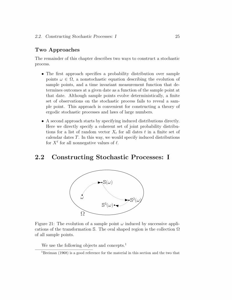
Figure 21: The evolution of a sample point ω induced by successive appli-cations of the transformation S. The oval shaped region is the collection Ωof all sample points.

We use the following objects and concepts.1

1Breiman (1968) is a good reference for the material in this section and the two that


S(ω)ω

Ω

Λ

S−1(Λ)

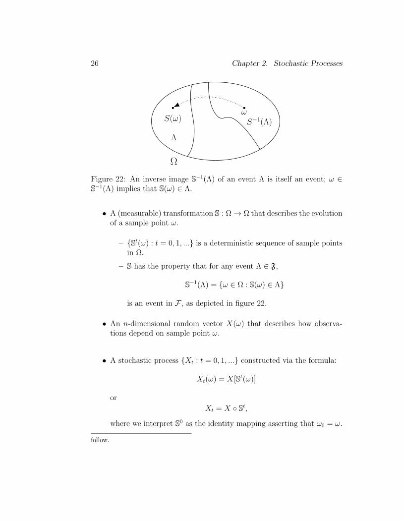
Figure 22: An inverse image S−1(Λ) of an event Λ is itself an event; ω ∈S−1(Λ) implies that S(ω) ∈ Λ.

• A (measurable) transformation S : Ω→ Ω that describes the evolutionof a sample point ω.

– St(ω) : t = 0, 1, ... is a deterministic sequence of sample pointsin Ω.

– S has the property that for any event Λ ∈ F,

S−1(Λ) = ω ∈ Ω : S(ω) ∈ Λ

is an event in F , as depicted in figure 22.

• An n-dimensional random vector X(ω) that describes how observa-tions depend on sample point ω.

• A stochastic process Xt : t = 0, 1, ... constructed via the formula:

Xt(ω) = X[St(ω)]

or

Xt = X St,

where we interpret S0 as the identity mapping asserting that ω0 = ω.

follow.

2.3. Stationary Stochastic Processes 27

Because a known function S maps a sample point ω ∈ Ω today into asample point S(ω) ∈ Ω tomorrow, the evolution of sample points is deter-ministic: for all j ≥ 1, ωt+j can be predicted perfectly if we know S and ωt.But we do not observe ωt at any t. Instead, we observe an (n × 1) vectorX(ω) that contains incomplete information about ω. We assign proba-bilities Pr to collections of sample points ω called events, then use thefunctions S and X to induce a joint probability distribution over sequencesof X’s. The resulting stochastic process Xt : 0 = 1, 2, ... is a sequence ofn-dimensional random vectors.

While this way of constructing a stochastic process may seem very spe-cial, the following example and section 2.9 show that it is not.

Example 2.2.1. Let Ω be a collection of infinite sequences of elements ofrt ∈ Rn so that ω = (r0, r1, ...), S(ω) = (r1, r2, ...), and X(ω) = r0. ThenXt(ω) = rt.

The S in example 2.2.1 is called the shift transformation. The triple (Ω,S, X)in example 2.2.1 generates an arbitrary sequence of (n× 1) vectors. We de-fer describing constructions of the events F and the probability measure Pruntil Section 2.9.

2.3 Stationary Stochastic Processes

In a deterministic dynamic system, a stationary state or steady state re-mains invariant as time passes. A counterpart of a steady state for astochastic process is a joint probability distribution that remains invari-ant over time in the sense that for any finite integer `, the probability dis-tribution of the composite random vector [Xt+1

′, Xt+2′, ..., Xt+`

′]′

does notdepend on t. We call a process with such a joint probability distributionstationary.

Definition 2.3.1. A transformation S is measure-preserving relative toprobability measure Pr if

Pr(Λ) = PrS−1(Λ)

for all Λ ∈ F.


Notice that the concept of measure preserving is relative to a probabilitymeasure Pr. A given transformation S can be measure preserving relativeto one Pr and not relative to others. This feature will play an importantrole at several points below.

Proposition 2.3.2. When S is measure-preserving, probability distributionfunctions of Xt are identical for all t ≥ 0.

Suppose that S is measure preserving. Given X and an integer ` > 1,form a vector

X [`](ω).=

X0(ω)X1(ω)...

X`(ω)

.We can apply Proposition 2.3.2 to X [`] to conclude that the joint distribu-tion function of (Xt, Xt+1, ..., Xt+`) is independent of t for t = 0, 1, . . ..That this property holds for any choice of ` is equivalent to the pro-cess Xt : t = 1, 2, ... being stationary.2 Thus, the restriction that Sis measure preserving relative to Pr implies that the stochastic processXt : t = 1, 2, ... is stationary.

For a given S, we now illustrate how to construct a probability measurePr that makes S measure preserving and thereby induces stationarity. Inexample 2.3.3, there is only one Pr that makes S measure preserving, whilein example 2.3.4 there are many.

Example 2.3.3. Suppose that Ω contains two points, Ω = ω1, ω2. Con-sider a transformation S that maps ω1 into ω2 and ω2 into ω1: S(ω1) = ω2

and S(ω2) = ω1. Since S−1(ω2) = ω1 and S−1(ω1) = ω2, for S tobe measure preserving, we must have Pr(ω1) = Pr(ω2) = 1/2.

Example 2.3.4. Suppose that Ω contains two points, Ω = ω1, ω2 andthat S(ω1) = ω1 and S(ω2) = ω2. Since S−1(ω2) = ω2 and S−1(ω1) =ω1, S is measure preserving for any Pr that satisfies Pr(ω1) ≥ 0 andPr(ω2) = 1− Pr(ω1).

2Sometimes this property is called ‘strict stationarity’ to distinguish it from weakernotions that require only that some moments of joint distributions be independent oftime. What is variously called wide-sense or second-order or covariance stationarityrequires only that first and second moments of joint distributions are independent ofcalendar time.

2.4. Invariant Events and Conditional Expectations 29

The next example illustrates how to represent an iid sequence of zeros andones.

Example 2.3.5. Suppose that Ω = [0, 1) and that Pr is the uniform mea-sure on this interval. Let

S(ω) =

2ω if ω ∈ [0, 1/2)

2ω − 1 if ω ∈ [1/2, 1),

X(ω) =

1 if ω ∈ [0, 1/2)0 if ω ∈ [1/2, 1).

By a straightforward calculation, Pr X1 = 1|X0 = 1 = Pr X1 = 1|X0 = 0 =Pr X1 = 1 = 1/2. An analogous conclusion prevails for the event X1 =0, so X1 is statistically independent of X0. By extending this argument, itcan be shown that Xt : t = 0, 1, ... is a sequence of independent randomvariables.3

2.4 Invariant Events and Conditional

Expectations

In this section, we present a Law of Large Numbers that asserts that whenS is measure-preserving relative to Pr, time series averages converge.

Invariant events

We use the concept of an invariant event to understand how limit points oftime series averages relate to a conditional mathematical expectation.

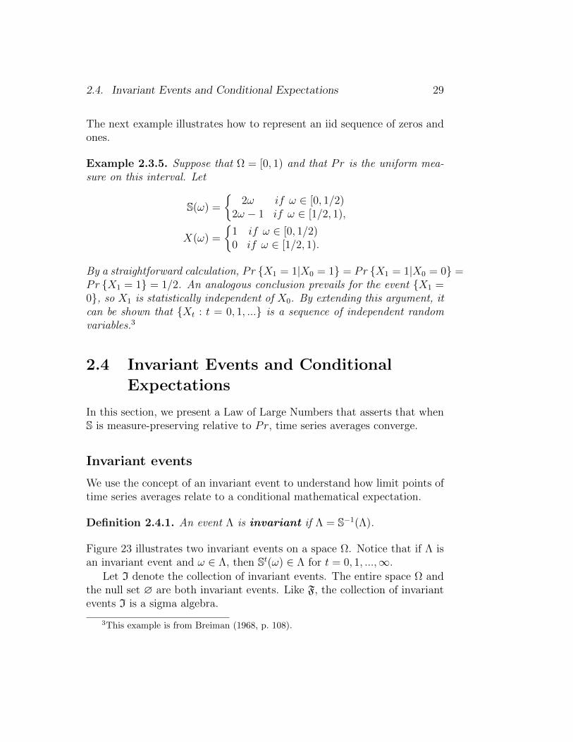
Definition 2.4.1. An event Λ is invariant if Λ = S−1(Λ).

Figure 23 illustrates two invariant events on a space Ω. Notice that if Λ isan invariant event and ω ∈ Λ, then St(ω) ∈ Λ for t = 0, 1, ...,∞.

Let I denote the collection of invariant events. The entire space Ω andthe null set ∅ are both invariant events. Like F, the collection of invariantevents I is a sigma algebra.

3This example is from Breiman (1968, p. 108).


Ω

Λ2 = S−1(Λ2)

Λ1 = S−1(Λ1)Λ3

Figure 23: Two invariant events Λ1 and Λ2 and an event Λ3 that is notinvariant.

Conditional expectation

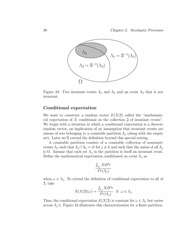
We want to construct a random vector E(X|I) called the “mathemati-cal expectation of X conditional on the collection J of invariant events”.We begin with a situation in which a conditional expectation is a discreterandom vector, an implication of an assumption that invariant events areunions of sets belonging to a countable partition Λj (along with the emptyset). Later we’ll extend the definition beyond this special setting.

A countable partition consists of a countable collection of nonemptyevents Λj such that Λj ∩Λk = ∅ for j 6= k and such that the union of all Λj

is Ω. Assume that each set Λj in the partition is itself an invariant event.Define the mathematical expectation conditioned on event Λj as∫

ΛjXdPr

Pr(Λj)

when ω ∈ Λj. To extend the definition of conditional expectation to all ofI, take

E(X|I)(ω) =

∫ΛjXdPr

Pr(Λj)if ω ∈ Λj.

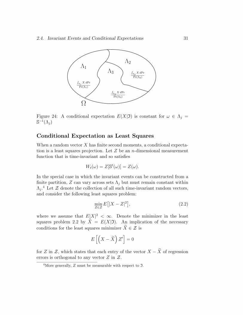
Thus, the conditional expectation E(X|I) is constant for ω ∈ Λj but variesacross Λj’s. Figure 24 illustrates this characterization for a finite partition.

2.4. Invariant Events and Conditional Expectations 31

Ω

Λ1

∫Λ1X dPr

Pr(Λ1)

Λ2

∫Λ2X dPr

Pr(Λ2)

Λ3

∫Λ3X dPr

Pr(Λ3)

Figure 24: A conditional expectation E(X|I) is constant for ω ∈ Λj =S−1(Λj)

Conditional Expectation as Least Squares

When a random vector X has finite second moments, a conditional expecta-tion is a least squares projection. Let Z be an n-dimensional measurementfunction that is time-invariant and so satisfies

Wt(ω) = Z[St(ω)] = Z(ω).

In the special case in which the invariant events can be constructed from afinite partition, Z can vary across sets Λj but must remain constant withinΛj.

4 Let Z denote the collection of all such time-invariant random vectors,and consider the following least squares problem:

minZ∈Z

E[|X − Z|2

], (2.2)

where we assume that E|X|2 < ∞. Denote the minimizer in the leastsquares problem 2.2 by X = E(X|I). An implication of the necessary

conditions for the least squares minimizer X ∈ Z is

E[(X − X

)Z ′]

= 0

for Z in Z, which states that each entry of the vector X − X of regressionerrors is orthogonal to any vector Z in Z.

4More generally, Z must be measurable with respect to I.


A measure-theoretic approach constructs a conditional expectation byextending the orthogonality property of least squares. Provided thatE|X| <∞, E(X|I) is the essentially unique random vector that, for any invariantevent Λ, satisfies

E ([X − E(X|I)]1Λ) = 0,

where 1Λ is the indicator function that is equal to one on the set Λ andzero otherwise.

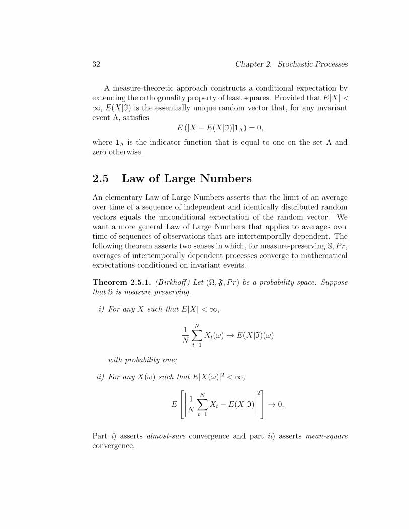
2.5 Law of Large Numbers

An elementary Law of Large Numbers asserts that the limit of an averageover time of a sequence of independent and identically distributed randomvectors equals the unconditional expectation of the random vector. Wewant a more general Law of Large Numbers that applies to averages overtime of sequences of observations that are intertemporally dependent. Thefollowing theorem asserts two senses in which, for measure-preserving S, P r,averages of intertemporally dependent processes converge to mathematicalexpectations conditioned on invariant events.

Theorem 2.5.1. (Birkhoff) Let (Ω,F, P r) be a probability space. Supposethat S is measure preserving.

i) For any X such that E|X| <∞,

1

N

N∑t=1

Xt(ω)→ E(X|I)(ω)

with probability one;

ii) For any X(ω) such that E|X(ω)|2 <∞,

E

∣∣∣∣∣ 1

N

N∑t=1

Xt − E(X|I)

∣∣∣∣∣2→ 0.

Part i) asserts almost-sure convergence and part ii) asserts mean-squareconvergence.

2.5. Law of Large Numbers 33

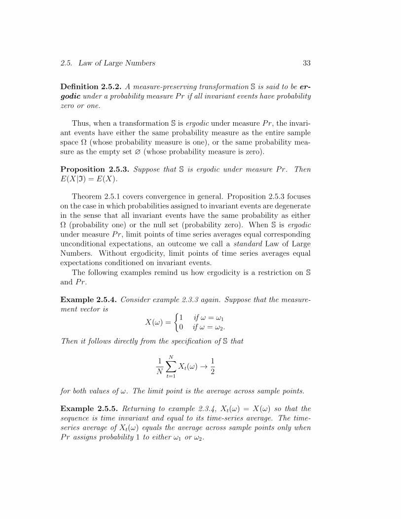
Definition 2.5.2. A measure-preserving transformation S is said to be er-godic under a probability measure Pr if all invariant events have probabilityzero or one.

Thus, when a transformation S is ergodic under measure Pr, the invari-ant events have either the same probability measure as the entire samplespace Ω (whose probability measure is one), or the same probability mea-sure as the empty set ∅ (whose probability measure is zero).

Proposition 2.5.3. Suppose that S is ergodic under measure Pr. ThenE(X|I) = E(X).

Theorem 2.5.1 covers convergence in general. Proposition 2.5.3 focuseson the case in which probabilities assigned to invariant events are degeneratein the sense that all invariant events have the same probability as eitherΩ (probability one) or the null set (probability zero). When S is ergodicunder measure Pr, limit points of time series averages equal correspondingunconditional expectations, an outcome we call a standard Law of LargeNumbers. Without ergodicity, limit points of time series averages equalexpectations conditioned on invariant events.

The following examples remind us how ergodicity is a restriction on Sand Pr.

Example 2.5.4. Consider example 2.3.3 again. Suppose that the measure-ment vector is

X(ω) =

1 if ω = ω1

0 if ω = ω2.

Then it follows directly from the specification of S that

1

N

N∑t=1

Xt(ω)→ 1

2

for both values of ω. The limit point is the average across sample points.

Example 2.5.5. Returning to example 2.3.4, Xt(ω) = X(ω) so that thesequence is time invariant and equal to its time-series average. The time-series average of Xt(ω) equals the average across sample points only whenPr assigns probability 1 to either ω1 or ω2.


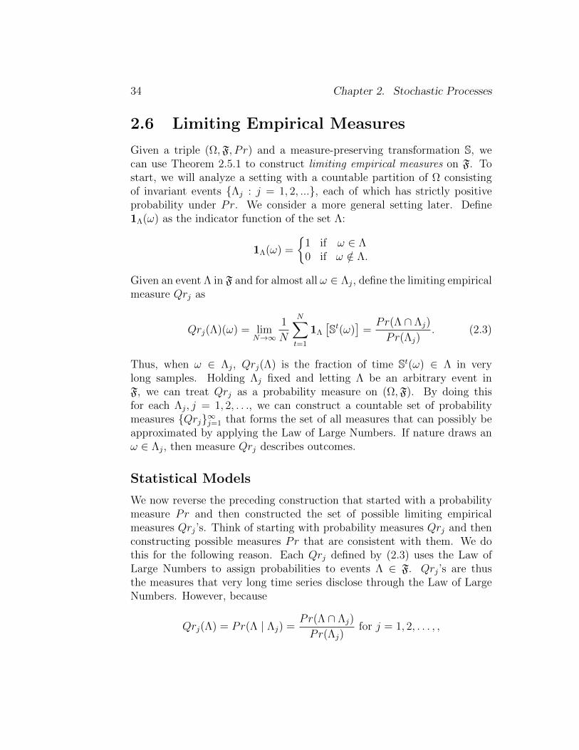
2.6 Limiting Empirical Measures

Given a triple (Ω,F, P r) and a measure-preserving transformation S, wecan use Theorem 2.5.1 to construct limiting empirical measures on F. Tostart, we will analyze a setting with a countable partition of Ω consistingof invariant events Λj : j = 1, 2, ..., each of which has strictly positiveprobability under Pr. We consider a more general setting later. Define1Λ(ω) as the indicator function of the set Λ:

1Λ(ω) =

1 if ω ∈ Λ0 if ω /∈ Λ.

Given an event Λ in F and for almost all ω ∈ Λj, define the limiting empiricalmeasure Qrj as

Qrj(Λ)(ω) = limN→∞

1

N

N∑t=1

1Λ

[St(ω)

]=Pr(Λ ∩ Λj)

Pr(Λj). (2.3)

Thus, when ω ∈ Λj, Qrj(Λ) is the fraction of time St(ω) ∈ Λ in verylong samples. Holding Λj fixed and letting Λ be an arbitrary event inF, we can treat Qrj as a probability measure on (Ω,F). By doing thisfor each Λj, j = 1, 2, . . ., we can construct a countable set of probabilitymeasures Qrj∞j=1 that forms the set of all measures that can possibly beapproximated by applying the Law of Large Numbers. If nature draws anω ∈ Λj, then measure Qrj describes outcomes.

Statistical Models

We now reverse the preceding construction that started with a probabilitymeasure Pr and then constructed the set of possible limiting empiricalmeasures Qrj’s. Think of starting with probability measures Qrj and thenconstructing possible measures Pr that are consistent with them. We dothis for the following reason. Each Qrj defined by (2.3) uses the Law ofLarge Numbers to assign probabilities to events Λ ∈ F. Qrj’s are thusthe measures that very long time series disclose through the Law of LargeNumbers. However, because

Qrj(Λ) = Pr(Λ | Λj) =Pr(Λ ∩ Λj)

Pr(Λj)for j = 1, 2, . . . , ,

2.6. Limiting Empirical Measures 35

such Qrj’s are only conditional probabilities and are silent about the prob-abilities Pr(Λj) of the underlying invariant events Λj. There are typicallymultiple choices of probabilities Pr that imply the same probabilities con-ditioned on invariant events.

Because Qrj’s are all that can ever be learned from “letting the dataspeak”, we regard each probability measure Qrj as a statistical model.

Definition 2.6.1. A statistical model is a probability measure that a Lawof Large Numbers can eventually disclose.

Therefore, for each invariant set Λj, the probability measure Qrj describesa statistical model.

Remark 2.6.2. For each j, S is measure-preserving and ergodic on (Ω,F, Qrj).In the second equality of definition (2.3), we assured ergodicity by assigningprobability one to the event Λj.

Relation (2.3) implies that probability Pr connects to probabilities Qrjby

Pr(Λ) =∑j

Qrj(Λ)Pr(Λj). (2.4)

Following as it does from definitions of the elementary objects comprisinga stochastic process, decomposition (2.4) is “just mathematics”. But itacquires special interest for us because it shows how to construct alternativeprobability measures Pr for which S is measure preserving. Because longdata series disclose probabilities conditioned on invariant events to be Qrj,we must hold the Qrj’s fixed, but we can freely assign probabilities Prto the underlying invariant events Λj and in this way create a family ofprobability measures for which S is measure preserving.

Decomposition (2.4) is of interest to both frequentist and Bayesianstatisticians.

• Decomposition (2.4) tells frequentist statisticians that when ω ∈ Λj

they can learn a particular Qrj, but not Pr.

• Decomposition (2.4) tells Bayesian statisticians how to represent theprobability measure Pr as a mixture of statistical models with weightsPr(Λj) interpretable as prior probabilities over statistical models.5

5The assertions in these two bullet points summarize a conversation between fre-quentist and Bayesian statisticians imagined by Kreps (1988, Ch. 11).


We extend these ideas in the following section.

2.7 Ergodic Decomposition

Earlier we started with a triple (Ω,F, P r) and then studied properties of al-ternative measure-preserving transformations S . To obtain a generalizationof decomposition (2.4), it is fruitful to explore consequences of a differentstarting point using a mathematical structure of Dynkin (1978). The ideais to begin with a transformation S and then to study a set of probabilitymeasures Pr for which S is both measure-preserving and ergodic.

We start with a pair (Ω,F). We assume that there is a metric on Ω andthat Ω is separable. We also assume that F is the collection of Borel sets(the smallest sigma algebra containing the open sets). Given (Ω,F), take a(measurable) transformation S and consider the set P of probability mea-sures Pr for which S is measure-preserving. For some of these probabilitymeasures, S is ergodic, but for others it is not. Let Q denote the set ofprobability measures for which S is ergodic. Under a nondegenerate con-vex combination of two probability measures in Q, S is measure-preservingbut not ergodic. Dynkin (1978) constructs limiting empirical measures Qron Q and justifies the following representation of the set P of probabilitymeasures Pr.

Proposition 2.7.1. For each probability measure P r in P there is a uniqueprobability measure π over Q such that

P r(Λ) =

∫QQr(Λ)π(dQr) (2.5)

for all Λ ∈ F.6

This proposition generalizes representation (2.4). It asserts a sense in whichthe set P of probabilities for which S is measure-preserving is convex. Theextremal points of this set are in the smaller set Q of probability measuresfor which the transformation S is ergodic. Representation (2.5) shows that

6Krylov and Bogolioubov (1937) give an early statement of this result. Dynkin (1978)provides a more general formulation that nests this and other closely related results.His analysis includes a formalization of integration over the probability measures in Q.Dynkin (1978) uses the resulting representation to draw connections between collectionsof invariant events and sets of sufficient statistics.

2.7. Ergodic Decomposition 37

by forming “mixtures” (i.e., weighted averages or convex combinations) ofprobability measures under which S is ergodic, we can represent all proba-bility specifications for which S is measure-preserving.

Practical model building

Like its specialized counterpart (2.4), representation (2.5) offers insightsabout building and interpreting probability models. As in section 2.6, wecan appeal to the Law of Large Numbers to interpret the probabilities inQ as statistical models that are components of a more complete probabilityspecification.7

A collection of invariant events I is associated with S. Formally, Dynkin(1978) shows that there exists a common conditional expectation operatorJ ≡ E(·|I) that assigns mathematical expectations to bounded measurablefunctions (mapping Ω into R) conditioned on the set of invariant eventsI. The conditional expectation operator J characterizes limit points oftime series averages of φ(Xt) for bounded functions φ for any Pr ∈ P .Alternative probability measures Pr assign different probabilities to theinvariant events.

Exchangeability

To explore connections between Proposition 2.7.1 and ideas of de Finettiand Hewitt and Savage, we begin with exchangeability property that ajoint probability distribution is invariant to rearrangements of the order ofobservations attained via a permutation of time indexes. de Finetti (1937)and Hewitt and Savage (1955) showed that exchangeability is a naturalconcept for elementary problems of statistical learning. Proposition 2.7.1extends exchangeability in ways that are especially useful for time seriesapplications.

7Marschak (1953), Hurwicz (1962), Lucas (1976), and Sargent (1981) distinquishedbetween structural econometric models and what we call statistical models. Structuraleconometric models are designed to forecast outcomes of hypothetical experiments thatfreeze some components of an economic environment while changing others. This requiresmore than representation 2.6 of a given stochastic process. A structural model invitesexperiments that alter statistical models.


Definition 2.7.2. A permutation of the time index is a one-to-one mappingof the set of nonnegative integers into itself.

Definition 2.7.3. A sequence of random vectors Xt : t = 0, 1, ... issaid to be exchangeable if joint probability distributions induced by this se-quence equal those for Xζ(0), Xζ(1), ... for any permutation ζ(0), ζ(1), . . .that keeps all but a finite number of indices fixed.8

A process is said to be exchangeable if joint distributions of members of thesequence Xt : t = 0, 1, ... do not depend on their order of appearance.

In section 2.7 we represented a probability measure P as the (convex)set of all probabilities under which S is measure-preserving. The set Pex ofall Pr for which Xt : t = 0, 1... is exchangeable is a (convex) subset ofP .9 More can be said. Let Qin denote the set of probabilities for which theprocess Xt : t = 1, 2, ... is independent and identically distributed. ThenQin ⊂ Pex. It happens that Q∩ Pex = Qin.

Proposition 2.7.1 represents probabilities in the set P of probabilitymeasures Pr for which S is measure-preserving in terms of ones in in therestricted set Q of probability measures under which S is ergodic. Similarly,a probability in Pex can be expressed as a weighted average of probabilitiesin Qin. de Finetti (1937) obtained this result for a setting with binary (zeroor one) random variables. Hewitt and Savage (1955) proved the followinggeneralization of de Finetti’s result:

Result 2.7.4. For each Pr in Pex there is a unique probability measure πover Qin such that

Pr(Λ) =

∫Qin

Qr(Λ)π(dQr) (2.6)

8An alternative but equivalent characterization of exchangeability due to Ryll-Nardzewski (1957) views exchangeable probabilities over Xt : t = 0, 1, ... as ones thatimply that the transformation S is measure-preserving under an associated Pr with addi-tional restrictions. Specifically, Ryll-Nardzewski shows that to establish exchangeability,it suffices to verify probabilistic invariance for specifications of ζ’s that map the nonneg-ative integers into the nonnegative integers and that satisfy ζ(0) < ζ(1) < ζ(2) < · · · .To establish stationarity, it suffices to verify this invariance under a more restrictivespecification ζ(j) = j + τ for j = 0, 1, 2, ... for any τ ≥ 1.

9Given (Ω,F) and the random vector X, the set Pex could be empty. For instance,provided that X differs across the two values of ω in example 2.3.3, there is no speci-fication of Pr for which Xt : t = 0, 1, ... is exchangeable. In contrast, all admissiblespecifications of Pr in example 2.3.4 imply that Xt : t = 0, 1, ... is exchangeable.


for all Λ ∈ F.

Thus, when we restrict the set of probabilities to be exchangeable, extremalpoints of the set become probabilities under which Xt : t = 1, 2, ... isindependent and identically distributed.

Foundations of statistics

The Law of Large Numbers stated in Theorem 2.5.1 and the Hewitt andSavage Result 2.7.4 provide foundations for both Bayesian and frequentiststatistics.10 Because we are interested in temporally dependent processes,we prefer to rely on foundations cast in a more general setting than al-lowed by exchangeability. Consequently, we feature stationarity instead ofexchangeability, so representation (2.5) in proposition 2.7.1 provides thefoundations that interest us.

Risk and uncertainty

We have adopted a frequentist notion of a statistical model based on a law oflarge numbers. An applied researcher typically does not know the statisticalmodel and so does not know limits of time-series averages.11 Instead, heor she faces uncertainty about which statistical model generated the data.This situation leads us to specifications of S that are consistent with afamily P of probability models under which S is measure preserving and astochastic process is stationary. Representation (2.5) describes uncertaintyabout statistical models with a probability distribution π over the set ofmodels Q.

For a Bayesian, π is a subjective prior probability distribution that pinsdown a convex combination of “statistical models.”12 A Bayesian expresseshis trust in that convex combination of statistical models when he constructsa complete probability measure over outcomes and uses it to compute ex-pected utility.13 A Bayesian decision theory axiomatized by Savage makes

10Kreps (1988, Ch. 11) describes how de Finetti’s theorem underlies statistical theoriesof learning about an unknown parameter.

11This statement is half of the point of Kreps (1988, Ch. 11).12This subsection is motivated in part by the intriguing discussions of von Plato (1982)

and Cerreia-Vioglio et al. (2013).13Here ‘complete’ can be taken to be synonymous with ‘not conditioning on invariant

events’.


no distinction between how decision makers respond to the probabilitiesembedded in the individual component statistical models and the π prob-abilities that he uses to mix them. All that matters to a Bayesian decisionmaker is his complete probability distribution over outcomes, not how it isattained as a π-mixture of component statistical models.

Some decision and control theorists challenge the complete confidencein a single prior probability assumed in a Bayesian approach.14 As an alter-native, they imagine decision makers who want to evaluate decisions underalternative π’s as a way to distinguish ‘uncertainty’, meaning ignorance ofπ, from ‘risk’, meaning prospective outcomes with probabilities reliably de-scribed by a given statistical model. This connects to ideas of Knight (1921)if we regard Knight as using “risk” to refer to ignorance that is completelydescribed by probabilities affiliated with a particular statistical model. ALaw of Large Numbers eventually discloses probabilities associated with aparticular statistical model. The π probabilities that a Bayesian uses to mixstatistical models are not revealed by a Law of Large Numbers. They are‘in the head of the decision maker.’ Bayes’ rule allows the decision makerto update the π probabilities as data accrue. As data accrue without limit,conditional probabilities over statistical models will eventually concentrateon the statistical model that generates the data.

Thus, while a Bayesian statistician knows a prior distribution Pr(Λj) :j = 1, 2, ... in representation (2.4), a statistician who doesn’t know Pr(Λj) :j = 1, 2, ... might want to explore the sensitivity of inferences to alterna-tive prior probability distributions. A robust Bayesian approach studiesthe consequences of changing the Pr(Λj)’s without altering the baselinestatistical models Qrj. Relatedly, Segal (1990) and Klibanoff et al. (2005)model decision makers who respond differently to ignorance summarized byπ than they do to the Knightian risk described by a particular statisticalmodel. Their decision makers refuse to reduce the compound lottery in-duced by π as is done in decomposition (2.6). Later, we will suggest waysto alter how models are weighted based on decomposition (2.4) along linessketched in Problem 1.5.1 in Chapter 1. In such cases doubts about themodel specification typically will be resolved by the Law of Large Num-bers, in effect revealing probabilities conditioned on invariant events. Insome the examples that interest us, it will take a long time to reveal theseconditional probabilities. We will also consider other formulations that will

14For example, see Hansen and Sargent (2008).


prevent the Law of Large Numbers from revealing the a unique statisticalmodel governing the data generation. Model ambiguity will not resolved,even asymptotically, in these examples.

Relationship to Misspecification Analysis

Sims (1971a,b, 1972, 1974, 1993), White (1994), and Hansen and Sargent(1993) studied limiting behavior of estimators of incorrect probability spec-ifications. To do that, they extended the settings of section 2.7 to capturethe idea that the econometrician’s ignorance goes beyond ‘not knowing aprior’.

To extend our formalism to include a misspecification analysis, let aneconometrician’s model of a stochastic process for Xt : t = 0, 1, ... bespecified in terms of a sample space and sigma algebra (Ω,F), a transfor-mation S, and a set Qm ⊂ Q of probability measures Pr for which S ismeasure-preserving and ergodic. The statistical models considered by theeconometrician are members of Qm. Often these can be represented interms of alternative possible values of an unknown parameter vector. ABayesian econometrician constructs a probability measure Prm in P thatis a mixture of the probability measures in Qm.

Unbeknownst to the econometrician, the data are actually generated bya probability model Prc for which S is measure-preserving and ergodic butthat is not in the econometrician’s set of possible models Qm. The econo-metrician’s specification and the true data generating model share compo-nents (Ω,F) of the probability space along with the transformation S andmeasurement function X. Because the actual data generating mechanism isPrc ∈ Q, it has an associated law of large numbers. But this true statisticalmodel is excluded from the econometrician’s set of statistical models Qm.Papers in the misspecification literature condition on the true statisticalmodel Prc and then study the consequences of applying statistical proce-dures like maximum likelihood to the econometrician’s probability modelor family of probability models. For example, some of these papers work ina frequentist tradition and show how probability limits of maximum like-lihood estimators of parameters for the econometrician’s model depend onfeatures of the true model Prc missed by the econometrician’s probabilitymodel.

Papers in this literature investigate consequences of i) assuming an ad-


mittedly false too tightly parameterized family of models,15 and ii) filteringdata in ways that eradicate seasonal or low frequency components of timeseries data to be used to estimate parameters of an economic model that isnot well designed to confront these components.16

2.8 Calibrators and econometricians

Decomposition (2.5) indicates how laws of large numbers condition on in-variant events. Unknown parameters that remain constant through time arekey invariant events for macroeconomists. Decomposition (2.5) in propo-sition 2.7.1 sheds light on distinct practices of macroeconomic calibratorsand econometricians.

Calibrators

Calibrators appeal to laws of large numbers to justify their ways of com-paring theories to observations. Calibrating a statistical model with freeparameters Θ = [θ1, . . . , θn] usually consists of these steps:

• Partition parameters Θ into two sets Θ1 and Θ2.

• Import parameters in subset Θ1 from earlier studies, including onesthat may have used different statistical models, and treat them asknown.17

• Given the parameters in Θ1, compute theoretical values of the Qrj’simplied by an economic model as functions of parameters in subsetΘ2. Here is one place that calibrators apply laws of large numbers.

• Set parameters in subset Θ2 to make a list of population momentsof the pertinent conditional distribution Qrm equal observed (finite)sample moments.

• Use the Qrm that emerges from the previous steps to compute pop-ulation moments of some random variables not used to calibrate the

15See Sims (1971a,b, 1972) and White (1994).16See Sims (1974, 1993), Wallis (1974), and Hansen and Sargent (1993).17Kuh and Meyer (1957) and Browning et al. (1999) criticize importing parameter

estimates inferred from one econometric specification into another.

2.8. Calibrators and econometricians 43

model. (Here is another step that uses a law of large numbers.) Com-pare these population moments with observed finite sample momentsas a basis either for validating the model or for uncovering “puzzles”(i.e., failures of the statistical model to fit some dimensions of thedata.)

A macroeconomic calibrator expresses no uncertainty about parametervalues. For him, parameter uncertainty is a distraction that he sets aside inorder to answer what he regards as more important questions. He pretendsto know parameters (i.e., he conditions on invariant events) and then makesstatements about economic outcomes implied by a given statistical model.He uses these outcomes to determine dimensions along which he judges hisstatistical model to be ‘successful’ and those along which he judges it to be‘deficient’. In this way he divides outcomes into scientific ‘understandings’and ‘puzzles’.18

Frequentists and Bayesians

While calibrators treat calibrated probabilities Qrm as known, econometri-cians confront the fact that finite data don’t contain enough informationreliably to pin down invariant events. All econometricians seek to quantifyuncertainty about parameters and the statistical models associated withthem, something that is not part of calibrators’ practice. But frequentistand Bayesian econometricians quantify uncertainty in different ways. Un-willing or unable to assign a prior distribution, a frequentist econometricianinvestigates consequences of conditioning on alternative statistical modelsin order to make inferences about sample statistics. A Bayesian econome-trician asserts a more complete probabilistic description of his uncertaintythan does a frequentist. He accomplishes this by representing his initial un-certainty over statistical models with a prior probability distribution andthen revising those probabilities by conditioning on available data.19

18See Mehra and Prescott (1985) and Lucas (2003) for prominent examples.19Kydland and Prescott (1996), Hansen and Heckman (1996), and Sims (1996) discuss

calibration.


Calibrators and Frequentists

Despite differences in their purposes and practices, macroeconomic calibra-tors and frequentist econometricians both condition on statistical models.As we have mentioned, calibrators appeal to a Law of Large Numbers as-sociated with a particular statistical model to justify how they set parame-ters. Frequentists use the Law of Large Numbers to understand the limitingbehaviors of sample statistics under alternative models. Thus, after condi-tioning on invariant events, frequentist econometricians and macroeconomiccalibrators proceed to do very different things. A frequentist econometricianconditions on a statistical model, then approximates the sample distribu-tions of particular statistics by using both a Law of Large Numbers and aCentral Limit Theorem.20 The frequentist uses those sampling distributionsto make probability statements conditioned on alternative models. That isthe frequentist econometrician’s way of describing his uncertainty aboutparameters and about the plausibility of alternative statistical models afterobserving a data sample.

2.9 Constructing Stochastic Processes: II

In section 2.2, we studied stochastic processes by using a transformation Sand a measure Pr on a canonical probability space (Ω,F). From there weinferred a collection of induced distributions. In practice, it can be moreconvenient to go the other direction by beginning with a set of inducedconditional distributions or joint distributions associated with collections ofcalendar dates and to restrict the distributions to be temporally consistent.From these, we can work backwards to construct a canonical representationof a stochastic process in terms of a triple (Ω,F, P r) and the transformationS that we used to illustrate things in section 2.1. There we let the set ofsample points Ω be a collection of infinite sequences of elements of Rn

with typical element ω = (r0, r1, ...), S(ω) = (r1, r2, ...), and X(ω) = r0.When we take the measurement to be Xt(ω) = rt, the transformation S canappropriately be called a shift transformation. To assign probabilities, fixan integer ` > 0. Let Pr` assign probabilities to the Borel sets of Rn(`+1).Pr` assigns probabilities to two mathematical objects. The first object is

20Calibrators rarely use or cite central limit theorems; these contain information aboutrates at which approximations based on laws of large numbers become reliable.

2.10. Inventing an infinite past 45

the composite random vector:

X [`](ω).=

X0(ω)X1(ω)

...X`(ω)

.The second object consists of a set of events in F that restrict the first` + 1 entries of ω = (r0, r1, ...), namely, events of a form given in (2.1). Toconstruct Pr and a stochastic process Xt : t = 0, 1, ..., we must specifyPr` for all nonnegative integers ` and make sure that Pr`+1 is consistentwith Pr` in the sense that both assign the same joint distribution to X [`].An alternative way to express consistency is to require that both Pr` andPr`+1 assign identical probabilities to events of the form Λ given in (2.1).If consistency in this sense prevails, then the Kolmogorov Extension Theo-rem guarantees that there exists a probability Pr on the space (Ω,F) thatis consistent with the probability assignments implied by Pr` for all non-negative integers `. In applications, we seek convenient ways to constructprobabilities Pr on Ω, while requiring that Pr` for ` = 0, 1, ... are consistentso that we can apply mathematical results from sections 2.2-2.7.

When S is measure-preserving, the probability distribution of the ran-dom vector [Xt

′, Xt+1′, ..., Xt+`

′]′

does not depend on t for any nonnegativeinteger `, so the process is stationary. Under the section 2.2 method ofconstructing a stochastic process, the result has a converse. Suppose Pr isspecified so that Xt : t = 1, 2, ... is stationary. Then the shift transfor-mation S in the canonical construction is measure-preserving.

Remark 2.9.1. We could have used the induced distributions for Xt :t = 0, 1, . . . to depict a probabilistically equivalent process in terms of ameasure-preserving probability on the canonical probability space describedat the outset of this chapter. But for central limit approximations and otherapplications too, it can be more convenient to invent an infinite past.

2.10 Inventing an infinite past

When Pr is measure preserving and the process Xt : t = 0, 1, ... is sta-tionary, it can be useful to invent an infinite past. To accomplish this, we


reason in terms of the (measurable) transformation S : Ω → Ω that de-scribes the evolution of a sample point ω. Until now we have presumedthat S has the property that for any event Λ ∈ F,

S−1(Λ) = ω ∈ Ω : S(ω) ∈ Λ

is an event in F. In this section and throughout chapter 5 too we alsoassume that S is one-to-one and has the property that for any event Λ ∈ F,

S(Λ) = ω ∈ Ω : S(ω) ∈ Λ ∈ F. (2.7)

BecauseXt(ω) = X[St(ω)] = Xt = X St

is well defined for negative values of t, restrictions 2.7 allow us to constructa “two-sided” process that has both an infinite past and an infinite future.Let A be a subsigma algebra of F, and let

At =

Λt ∈ F : Λt = ω ∈ Ω : St(ω) ∈ Λ for some Λ ∈ F.

We assume that At : −∞ < t < +∞ is a nondecreasing filtration.If the original measurement function X is A-measurable, then Xt is At-measurable. Furthermore, Xt−j is in At for all j ≥ 0. The set At depictsinformation available at date t, including past information. The invariantevents in I are contained in At for all t.

We construct the following moving-average process in terms of an infinitehistory.

Example 2.10.1. (Moving average) Suppose that Wt : −∞ < t < ∞ isa vector stationary process for which

E (Wt+1|At) = 0

and that E (WtWt′|I) = I for all −∞ < t < +∞. One possibility is that

this sequence is i.i.d. Construct

Xt =∞∑j=0

αj ·Wt−j (2.8)

where∞∑j=0

|αj|2 <∞. (2.9)

2.10. Inventing an infinite past 47

Restriction (2.12) implies that Xt is well defined as a mean square limit.Xt is constructed from the infinite past Wt−j : 0 ≤ j < ∞. The processXt : −∞ < t < ∞ is stationary and is often called an infinite-ordermoving average process. The sequence αj : j = 0, 1, ... can depend on theinvariant events.


Appendix 2.A Frequency Domain

Representation

Processes having an infinite past can be analyzed in the frequency domain.Where z is a complex variable, the right side of

α(z) =∞∑j=0

αjzj

is a power series expansion of the complex-valued function α. We assumethat the power series converges for |z| < 1, a condition that is satisfiedwhen the function α is analytic on the set |z| < 1.

We care about the behavior of α(z) near the boundary z = 1. To studythis, it is convenient to invent a probability space and use it to constructa process having the same second moment processes as the original process(conditioned on invariant events). To show how to do this, suppose initially

that Wt : −∞ < t < +∞ is scalar. Let ω ∈ Ω = [0, 2π) and let P r denote

the uniform measure over Ω. Introduce a scalar complex valued process

Wt(ω) = exp(−iωt)

for all integers t. Where ∗ denotes complex conjugation, notice that

Wt

(Ws

)∗= exp [iω(s− t)]∣∣∣Wt

∣∣∣2 = 1.

Since1

2π

∫Ω

exp [iω(s− t)] = 0

for nonzero integer values of s − t, the processWt : −∞ < t < +∞

is

serially orthogonal. Moreover, the process has a unit second moment for allinteger t. We construct a process

Xt(ω) = exp(−ωt)α[exp(iω)]

that is well defined as a mean-square limit. Moreover, if we set z =ρ exp(iω), then for almost all ω, α[exp(iω)] is the limit of α(z) as ρ in-

2.B. Hidden Periodicity 49

creases to one. Using the convenient (Ω, P r) probability space, we compute

E∣∣∣Xt

∣∣∣2 =1

2π

∫Ω

|α[exp(iω)]|2 dω

=∞∑j=0

(αj)2 ,

where the second equality is known as Parseval’s formula. Moreover,

E[Xt

(Xt−s

)∗]=

1

2π

∫Ω

exp(−iωs) | α[exp(iω)] |2 dω

for any s. By construction:

E (XtXt−s|I) = E[Xt

(Xt−s

)∗]=

1

2π

∫Ω

exp(−iωs) | α[exp(iω)] |2 dω

The function | α[exp(iω)] |2 is called the spectral density of the Xt pro-cess.

Up to now we have assumed a scalar shock process. If there are multipleshocks that are uncorrelated, then we can repeat our calculations shock byshock. Now α(z) is vector of analytic functions

E (XtXt−s|I) =1

2π

∫Ω

exp(−iωs) | α[exp(iω)] |2 dω,

and | α[exp(iω)] |2=| α[exp(iω)]α′[exp(−iω)] | is the spectral density ma-trix.

Appendix 2.B Hidden Periodicity

Example 2.B.1. (Hidden periodicity) Suppose again that Wt : −∞ < t <∞ is a vector stationary process for which21

E (Wt+1|At) = 0

21This example extends Hansen and Sargent (1993) and Hansen and Sargent (2013,ch. 14), where we started with periodic autoregressive representations.


and that E (WtWt′|I) = I for all −∞ < t < +∞. Where p ≥ 2 is an integer

that we call the periodicity, let there be p matrix sequences of moving averagecoefficients, one for each “season” ` ∈ 1, 2, . . . , p. Suppose that

Xt =∞∑j=0

α`(t)j ·Wt−j (2.10)

where `(t + 1) = `(t) + 1 unless `(t) = p, in which case `(t + 1) = 1. Itfollows that

`(t+ p) = `(t) ∀t = 0,±1,±2, . . .. (2.11)

Assume that for each ` ∈ 1, 2, . . . , p∞∑j=0

|α`j|2 <∞. (2.12)

and calculate z-transforms

α`(z) =∞∑j=0

α`j(z)j

for ` = 1, 2, ..., p. When z-transform α`(z) applies at date t, α`+1(z) appliesat date t+ 1, modulo p, by which we mean that when αp(z) is the transformat date t, α1(z) is the transform at date t+ 1.

Whether the stochastic process Xt in (2.10) is stationary depends onhow we think of initializing ` at date t = 0. The following procedure initial-izes ` so that the process Xt is stationary: randomize ` at date t = 0 byletting ` be each possible value 1, . . . , p with probability 1/p. Then if theshock process is an i.i.d. vector sequence of standard normally distributedrandom vectors, the Xt process in (2.10) is stationary and ergodic. Thisstationary process has spectral density

1

p

p∑`=1

|α` [exp (iω)] |2

and associated inversion formula is

E (XtXt−s) =1

2π

∫Ω

exp(−iωs)

(1

p

p∑`=1

| α` [exp (iω)] |2)dω

2.B. Hidden Periodicity 51

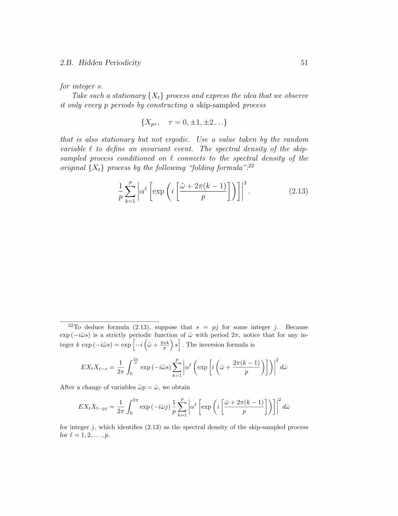
for integer s.Take such a stationary Xt process and express the idea that we observe

it only every p periods by constructing a skip-sampled process

Xpτ , τ = 0,±1,±2 . . .

that is also stationary but not ergodic. Use a value taken by the randomvariable ` to define an invariant event. The spectral density of the skip-sampled process conditioned on ` connects to the spectral density of theoriginal Xt process by the following “folding formula”:22

1

p

p∑k=1

∣∣∣∣α` [exp

(i

[ω + 2π(k − 1)

p

])]∣∣∣∣2 . (2.13)

22To deduce formula (2.13), suppose that s = pj for some integer j. Becauseexp (−iωs) is a strictly periodic function of ω with period 2π, notice that for any in-

teger k exp (−iωs) = exp[−i(ω + 2πk

p

)s]. The inversion formula is

EXtXt−s =1

2π

∫ 2πp

0

exp (−iωs)p∑k=1

∣∣∣∣α`(exp

[i

(ω +

2π(k − 1)

p

)])∣∣∣∣2 dωAfter a change of variables ωp = ω, we obtain

EXtXt−pj =1

2π

∫ 2π

0

exp (−iωj) 1

p

p∑k=1

∣∣∣∣α` [exp

(i

[ω + 2π(k − 1)

p

])]∣∣∣∣2 dωfor integer j, which identifies (2.13) as the spectral density of the skip-sampled processfor ` = 1, 2, . . . , p.

Chapter 2 Stochastic Processes - Lars Peter...

Documents

Transcript of Chapter 2 Stochastic Processes - Lars Peter...