CHAPTER 10: ESTIMATION AND HYPOTHESIS TESTING: TWO POPULATIONS.
RS – Chapter 2 – Random Variables 8/14/2019
1
Chapter 2
Random Variables
Random Variables
• A random variable is a convenient way to express the elements of Ω as numbers rather than abstract elements of sets.
Definition: Let AX; AY be nonempty families of subsets of X and Y, respectively. A function f: X → Y is (AX;AY )-measurable if f -1
A ∈ AX for all A ∈ AY.
Definition: Random Variable•A random variable X is a measurable function from the probability space (Ω, Σ ,P) into the probability space (χ, AX, PX), where χ in R is the range of X (which is a subset of the real line) AX is a Borel field of X, and PX is the probability measure on χ induced by X.Specifically, X: Ω→ χ.
RS – Chapter 2 – Random Variables 8/14/2019
2
Remarks:
- A random variable X is a function.
- It is a numerical quantity whose value is determined by a random experiment.
- It takes single elements in Ω and maps them to single points in R.
- P is the probability measure over the sample space and PX is the probability measure over the range of the random variable.
- The induced measure PX is just a way of relating measure on the real line –the range of X– back to the original probability measure over the abstract events in the σ-algebra of the sample space.
Random Variables - Remarks
Interpretation
The induced measure PX allows us to relate a measure on the real line –the range of X– back to the original probability measure over the abstract events in the σ-algebra of the sample space:
PX[A] = P [X-1(A)] =P[ω∈ Ω: X(ω) ∈ A.
That is, we take the probability weights associated with events and assign them to real numbers. Recall that when we deal with probabilities on some random variable X, we are really dealing with the PX measure.
We measure the "size" of the set (using P as our measure) of ω's such that the random variable X returns values in A.
Random Variables - Interpretation
RS – Chapter 2 – Random Variables 8/14/2019
3
Interpretation
P is the probability measure over the sample space and PX is the probability measure over the range of the random variable.
Thus, we write P[A] (where A is a subset of the range of X) but we
mean PX[A], which is equivalent to P[ω∈ Ω: X(ω) ∈ A].
Notational shortcut: We use P[A] instead of PX [A]
(This notation can be misleading if there's confusion about whether A is in the sample space or in the range of X.)
Random Variables - Interpretation
Example: Back to the previous example where two coins are tossed. We defined the sample space (Ω) as all possible outcomes and the sigma algebra of all possible subsets of the sample space. A simple probability measure (P) was applied to the events in the sigma algebra.
Let the random variable X be "number of heads." Recall that X
takes Ω into χ and induces PX from P. In this example, χ = 0; 1; 2 and A = Φ; 0; 1; 2; 0;1; 0;2; 1;2; 0;1;2.
The induced probability measure PX from the measure defined above would look like:
Random Variables – Example 1
RS – Chapter 2 – Random Variables 8/14/2019
4
Example: Back to the previous example where two coins are tossed.
Prob. of 0 heads = PX[0] = P[TT] = 1/4
Prob. of 1 heads = PX[1] = P[HT; TH] = 1/2
Prob. of 2 heads = PX[2] = P[HH] = ¼
Prob. of 0 or 1 heads = PX[0; 1] = P[TT; TH; HT] = 3/4
Prob. of 0 or 2 heads = PX[0; 2] = P[TT; HH] = 1/2
Prob. of 1 or 2 heads = PX[1; 2] = P[TH; HT; HH] = 3/4
Prob. of 1, 2, or 3 heads = PX[0; 1; 2] = P[HH; TH; HT; TT] = 1
Prob. of "nothing" = PX[Φ] = P[Φ] = 0
The empty set is simply needed to complete the σ-algebra. Its interpretation is not important since P[Φ] = 0 for any reasonable P.
Random Variables – Example 1
Example: Probability Space
One standard probability space is the Borel field over the unit interval of the real line under the Lebesgue measure λ. That is ([0, 1]; B; λ).
The Borel field over the unit interval gives us a set of all possible intervals taken from [0,1]. The Lebesgue measure measures the size of any given interval. For any interval [a; b] in [0,1] with b ≥ a,
λ[[a, b]] = b – a.
This probability space is well known: “uniform distribution,” the probability of any interval of values is the size of the interval.
Random Variables – Example 2
RS – Chapter 2 – Random Variables 8/14/2019
5
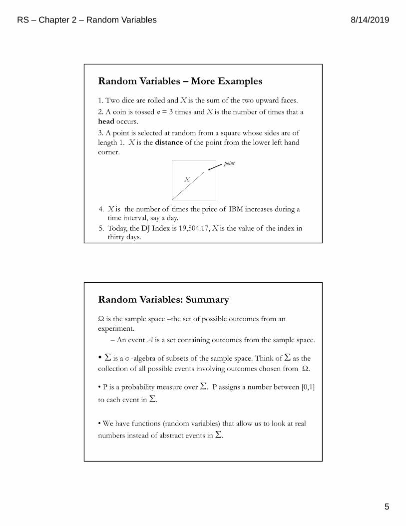
1. Two dice are rolled and X is the sum of the two upward faces.
2. A coin is tossed n = 3 times and X is the number of times that a head occurs.
3. A point is selected at random from a square whose sides are of length 1. X is the distance of the point from the lower left hand corner.
4. X is the number of times the price of IBM increases during a time interval, say a day.
5. Today, the DJ Index is 19,504.17, X is the value of the index in thirty days.
point
X
Random Variables – More Examples
Ω is the sample space –the set of possible outcomes from an experiment.
– An event A is a set containing outcomes from the sample space.
• Σ is a σ -algebra of subsets of the sample space. Think of Σ as the collection of all possible events involving outcomes chosen from Ω.
• P is a probability measure over Σ. P assigns a number between [0,1]
to each event in Σ.
• We have functions (random variables) that allow us to look at real
numbers instead of abstract events in Σ.
Random Variables: Summary
RS – Chapter 2 – Random Variables 8/14/2019
6
• For each random variable X, there exists a new probability measure
PX: PX [A] where A ∈ R simply relates back to P[ω∈ Ω: X(ω) ∈A.
We calculate PX[A], but we are really interested in the probability
P[ω∈ Ω: X(ω) ∈ A,
where A simply represents ω∈ Ω: X(ω) ∈ A through the inverse transformation X-1.
Random Variables: Summary
Definition – The probability function, p(x), of a RV, X.For any random variable, X, and any real number, x, we define
where X = x = the set of all outcomes (event) with X = x.
p x P X x P X x
Definition – The cumulative distribution function (CDF), F(x), of a RV, X.For any random variable, X, and any real number, x, we define
where X ≤ x = the set of all outcomes (event) with X ≤ x.
F x P X x P X x
Random Variables: Probability Function & CDF
RS – Chapter 2 – Random Variables 8/14/2019
7
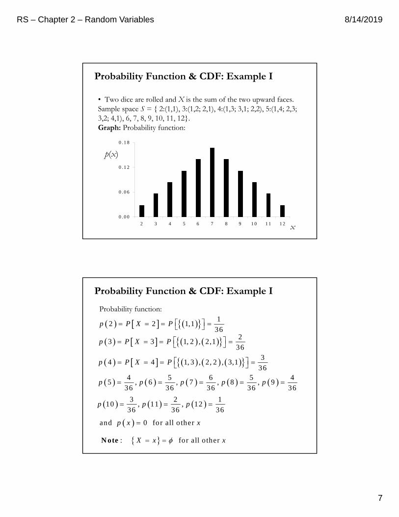
• Two dice are rolled and X is the sum of the two upward faces. Sample space S = 2:(1,1), 3:(1,2; 2,1), 4:(1,3; 3,1; 2,2), 5:(1,4; 2,3; 3,2; 4,1), 6, 7, 8, 9, 10, 11, 12.Graph: Probability function:
0 . 0 0
0 . 0 6
0 . 1 2
0 . 1 8
2 3 4 5 6 7 8 9 1 0 1 1 1 2 x
p(x)
Probability Function & CDF: Example I
12 2 1,1
36p P X P
23 3 1, 2 , 2,1
36p P X P
34 4 1, 3 , 2, 2 , 3,1
36p P X P
4 5 6 5 45 , 6 , 7 , 8 , 9
36 36 36 36 36p p p p p
3 2 110 , 11 , 12
36 36 36p p p
and 0 for all other p x x
: for all other X x x N ote
Probability function:
Probability Function & CDF: Example I
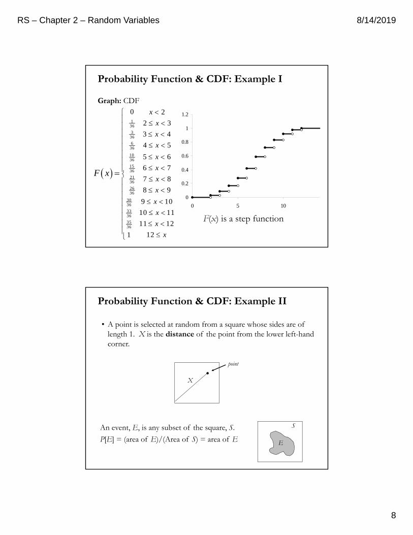
RS – Chapter 2 – Random Variables 8/14/2019
8
0
0.2
0.4
0.6
0.8
1
1.2
0 5 10
Graph: CDF
F x
136
336
636
1036
1536
2136
2636
3036
3336
3536
0 2
2 3
3 4
4 5
5 6
6 7
7 8
8 9
9 10
10 11
11 12
121
x
x
x
x
x
x
x
x
x
x
x
x
F(x) is a step function
Probability Function & CDF: Example I
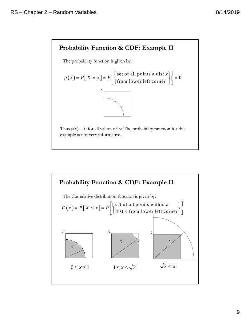
• A point is selected at random from a square whose sides are of length 1. X is the distance of the point from the lower left-hand corner.
An event, E, is any subset of the square, S.
P[E] = (area of E)/(Area of S) = area of E
point
X
S
E
Probability Function & CDF: Example II
RS – Chapter 2 – Random Variables 8/14/2019
9
Thus p(x) = 0 for all values of x. The probability function for this example is not very informative.
set of all points a dist 0
from lower left corner
xp x P X x P
S
The probability function is given by:
Probability Function & CDF: Example II
set of all poin ts w ith in a
d ist from low er left cornerF x P X x P
x
The Cumulative distribution function is given by:
S
0 1x 1 2x 2 x
xx x
Probability Function & CDF: Example II
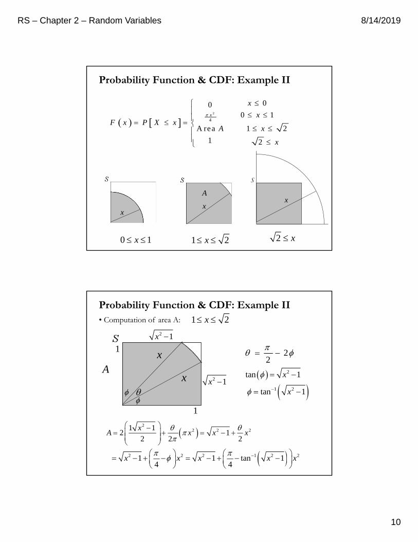
RS – Chapter 2 – Random Variables 8/14/2019
10
2
4
000 1
A rea 1 2
1 2
x
x
xF x P X x
A x
x
S
0 1x 1 2x 2 x
xx
xA
Probability Function & CDF: Example II
1 2x
xA
x1
22
2 1x
2 1x
2
2 2 21 12 1
2 2 2
xA x x x
2 2 2 1 2 21 1 tan 14 4
x x x x x
2tan 1x
1 2tan 1x
1
Probability Function & CDF: Example II
• Computation of area A:
RS – Chapter 2 – Random Variables 8/14/2019
11
0
1
-1 0 1 2
2
2 1 2 2
0 0
0 14
1 tan 1 1 24
1 2
x
xx
F x P X xx x x x
x
F x
Probability Function & CDF: Example II
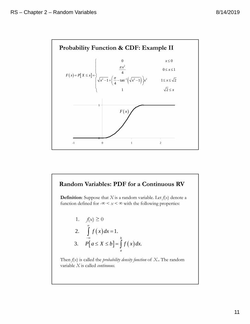
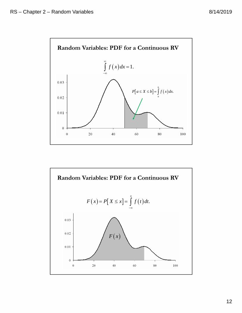
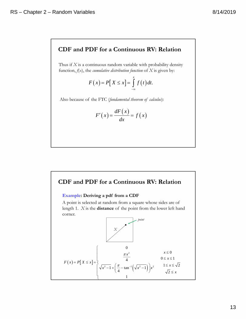
Definition: Suppose that X is a random variable. Let f(x) denote a function defined for -∞ < x < ∞ with the following properties:
1. f(x) ≥ 0
2. 1.f x dx
3. .
b
a
P a X b f x dx
Then f(x) is called the probability density function of X.. The random variable X is called continuous.
Random Variables: PDF for a Continuous RV
RS – Chapter 2 – Random Variables 8/14/2019
12
1.f x dx
.b
a
P a X b f x dx
Random Variables: PDF for a Continuous RV
F x
.x
F x P X x f t dt
Random Variables: PDF for a Continuous RV
RS – Chapter 2 – Random Variables 8/14/2019
13
Thus if X is a continuous random variable with probability density function, f(x), the cumulative distribution function of X is given by:
.x
F x P X x f t dt
Also because of the FTC (fundamental theorem of calculus):
dF xF x f x
dx
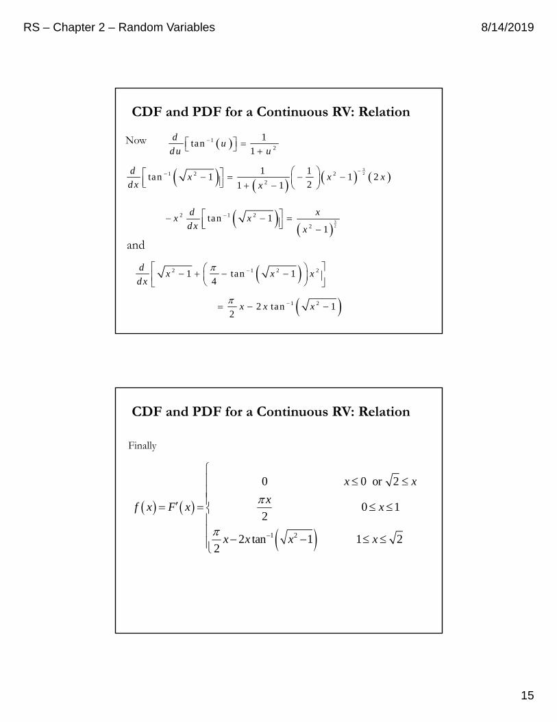
CDF and PDF for a Continuous RV: Relation
Example: Deriving a pdf from a CDF
A point is selected at random from a square whose sides are of length 1. X is the distance of the point from the lower left hand corner.
point
X
2
2 1 2 2
00
0 14 1 2
1 tan 14 2
1
xxx
F x P X xx
x x xx
CDF and PDF for a Continuous RV: Relation
RS – Chapter 2 – Random Variables 8/14/2019
14
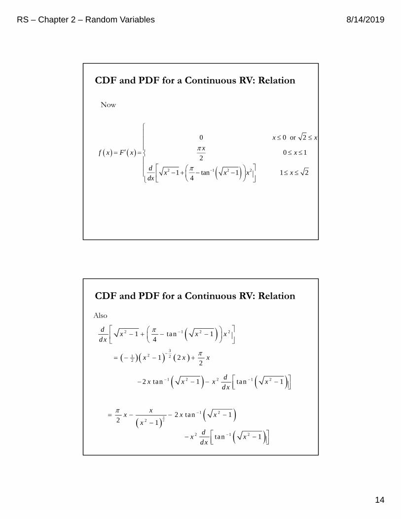
Now
2 1 2 2
0 0 or 2
0 12
1 tan 1 1 24
x x
xf x F x x
dx x x x
dx
CDF and PDF for a Continuous RV: Relation
2 1 2 21 tan 14
dx x x
dx
3
21 22 1 2
2x x x
1 2 2 1 22 tan 1 tan 1d
x x x xdx
Also
3
2
1 2
22 tan 1
2 1
xx x x
x
2 1 2tan 1d
x xdx
CDF and PDF for a Continuous RV: Relation
RS – Chapter 2 – Random Variables 8/14/2019
15
Now
321 2 2
2
1 1tan 1 1 2
21 1
dx x x
dx x
12
1tan
1
du
du u
and
32
2 1 2
2tan 1
1
d xx x
dx x
2 1 2 21 tan 14
dx x x
dx
1 22 tan 12
x x x
CDF and PDF for a Continuous RV: Relation
Finally
1 2
0 0 or 2
0 12
2 tan 1 1 22
x x
xf x F x x
x x x x
CDF and PDF for a Continuous RV: Relation
RS – Chapter 2 – Random Variables 8/14/2019
16
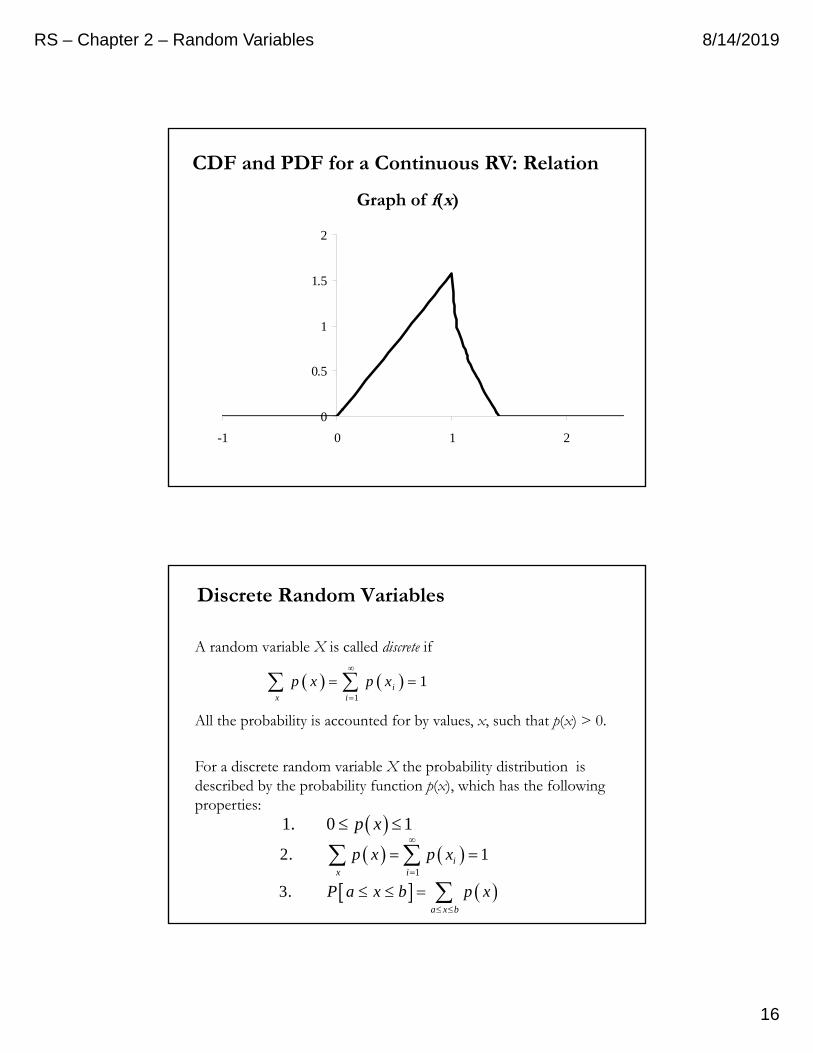
Graph of f(x)
0
0.5
1
1.5
2
-1 0 1 2
CDF and PDF for a Continuous RV: Relation
Discrete Random Variables
A random variable X is called discrete if
All the probability is accounted for by values, x, such that p(x) > 0.
For a discrete random variable X the probability distribution is described by the probability function p(x), which has the following properties:
1
1ix i
p x p x
1. 0 1p x
1
2. 1ix i
p x p x
3.
a x b
P a x b p x
RS – Chapter 2 – Random Variables 8/14/2019
17
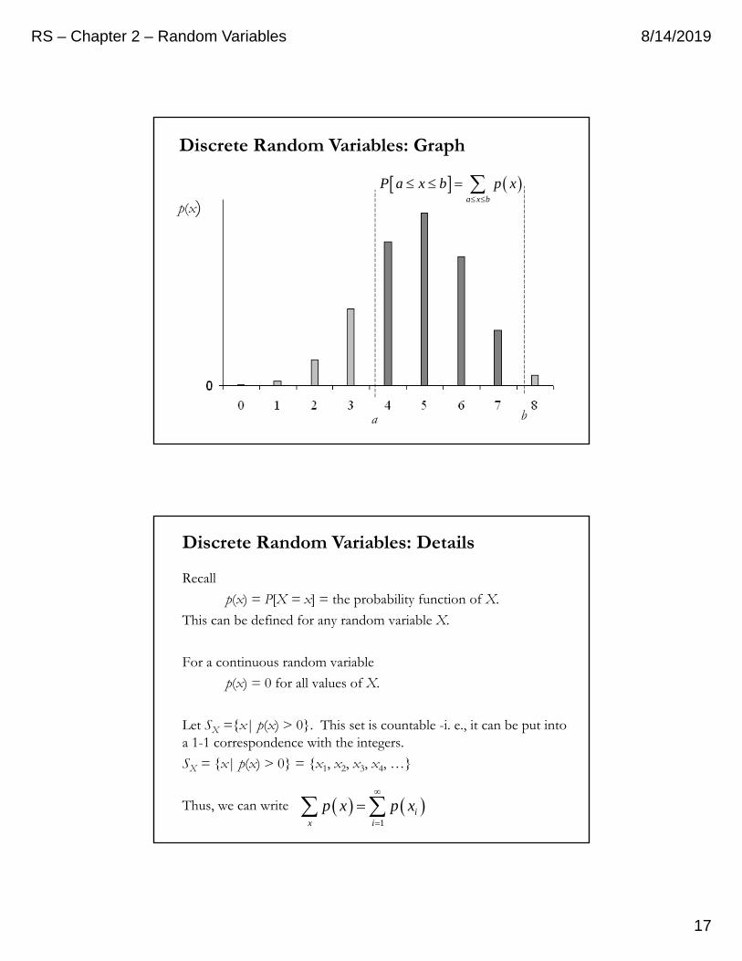
p(x)
a x b
P a x b p x
a b
Discrete Random Variables: Graph
Recall
p(x) = P[X = x] = the probability function of X.
This can be defined for any random variable X.
For a continuous random variable
p(x) = 0 for all values of X.
Let SX =x| p(x) > 0. This set is countable -i. e., it can be put into a 1-1 correspondence with the integers.
SX = x| p(x) > 0 = x1, x2, x3, x4, …
Thus, we can write 1
ix i
p x p x
Discrete Random Variables: Details
RS – Chapter 2 – Random Variables 8/14/2019
18
Thus the elements of SX = S1 S2 S3 S3 …
can be arranged x1, x2, x3, x4, …
by choosing the first elements to be the elements of S1 ,
the next elements to be the elements of S2 ,
the next elements to be the elements of S3 ,
the next elements to be the elements of S4 ,
etc
This allows us to write
1
for ix i
p x p x
Discrete Random Variables: Details
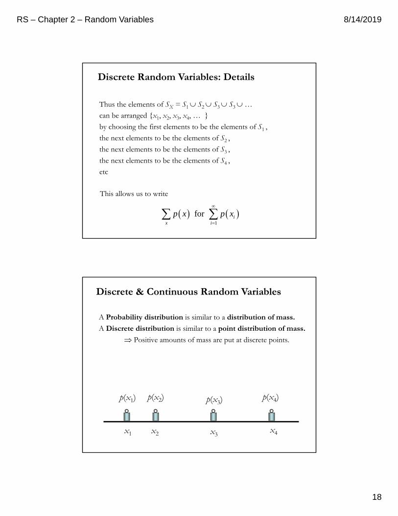
A Probability distribution is similar to a distribution of mass.
A Discrete distribution is similar to a point distribution of mass.
Positive amounts of mass are put at discrete points.
x1 x2 x3x4
p(x1) p(x2) p(x3) p(x4)
Discrete & Continuous Random Variables
RS – Chapter 2 – Random Variables 8/14/2019
19
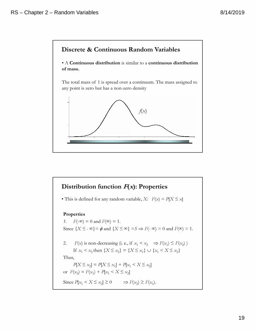
• A Continuous distribution is similar to a continuous distribution of mass.
The total mass of 1 is spread over a continuum. The mass assigned to any point is zero but has a non-zero density
f(x)
Discrete & Continuous Random Variables
Distribution function F(x): Properties
• This is defined for any random variable, X: F(x) = P[X ≤ x]
Properties
1. F(-∞) = 0 and F(∞) = 1.
Since X ≤ - ∞= and X ≤ ∞ =S F(- ∞) = 0 and F(∞) = 1.
2. F(x) is non-decreasing (i. e., if x1 < x2 F(x1) ≤ F(x2) )
If x1 < x2 then X ≤ x2 = X ≤ x1 x1 < X ≤ x2
Thus,
P[X ≤ x2] = P[X ≤ x1] + P[x1 < X ≤ x2]
or F(x2) = F(x1) + P[x1 < X ≤ x2]
Since P[x1 < X ≤ x2] ≥ 0 F(x2) ≥ F(x1).
RS – Chapter 2 – Random Variables 8/14/2019
20
3. F(b) – F(a) = P[a < X ≤ b].
If a < b then using the argument above
F(b) = F(a) + P[a < X ≤ b]
F(b) – F(a) = P[a < X ≤ b].
4. p(x) = P[X = x] =F(x) – F(x-)
Here, limu x
F x F u
5. If p(x) = 0 for all x (i.e., X is continuous) then F(x) is continuous. A function F is continuous if
lim limu x u x
F x F u F x F u
One can show that p(x) = 0 implies
F x F x F x
Distribution function F(x): Properties
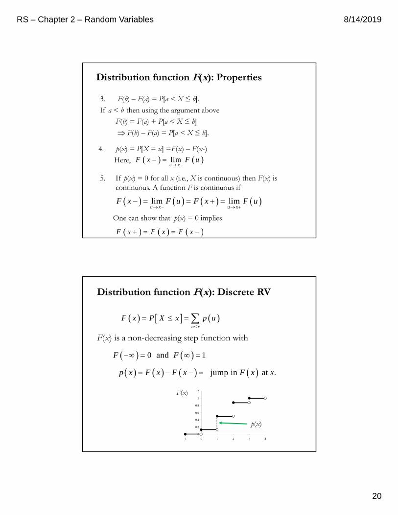
F(x) is a non-decreasing step function with
u x
F x P X x p u
jump in at .p x F x F x F x x
0 and 1F F
0
0.2
0.4
0.6
0.8
1
1.2
-1 0 1 2 3 4
F(x)
p(x)
Distribution function F(x): Discrete RV
RS – Chapter 2 – Random Variables 8/14/2019
21
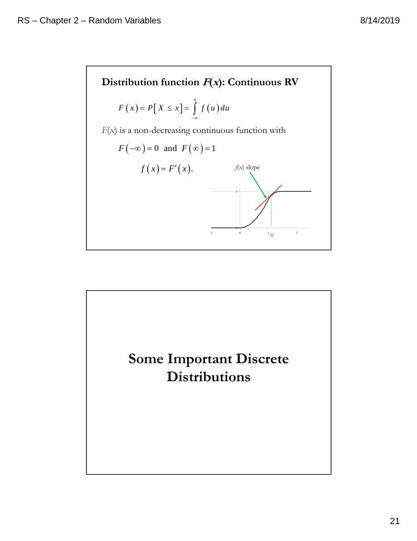
F(x) is a non-decreasing continuous function with
x
F x P X x f u du
.f x F x
0 and 1F F
F(x)
f(x) slope
0
1
-1 0 1 2x
Distribution function F(x): Continuous RV
Some Important Discrete Distributions
RS – Chapter 2 – Random Variables 8/14/2019
22
The Binomial distribution
Jacob Bernoulli (1654– 1705)
Suppose that we have a Bernoulli trial (an experiment) that has 2 results:1. Success (S)2. Failure (F)
Suppose that p is the probability of success (S) and q = 1 – p is the probability of failure (F). Then, the probability distribution with probability function
0
1
q xp x P X x
p x
is called the Bernoulli distribution.
• Now assume that the Bernoulli trial is repeated independently n times.Let X be the number of successes ocurring in the n trials. (The possible values of X are 0, 1, 2, …, n)
Bernouille Distribution
RS – Chapter 2 – Random Variables 8/14/2019
23
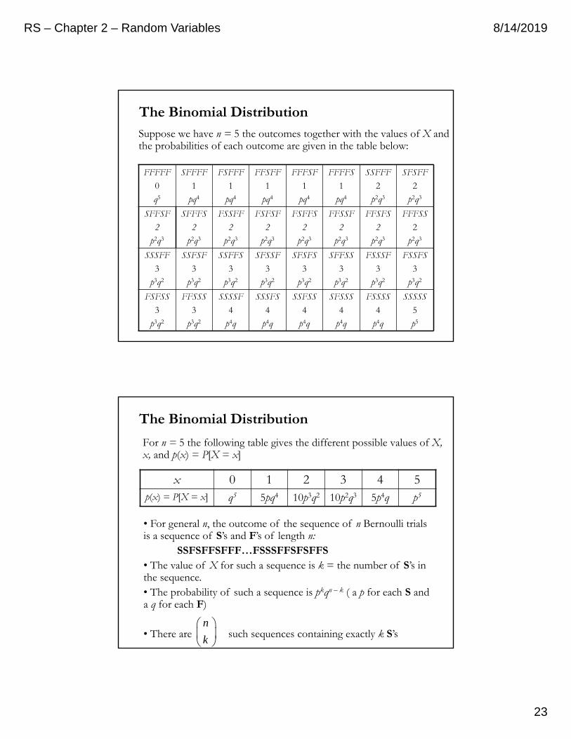
Suppose we have n = 5 the outcomes together with the values of X and the probabilities of each outcome are given in the table below:
FFFFF
0
q5
SFFFF
1
pq4
FSFFF
1
pq4
FFSFF
1
pq4
FFFSF
1
pq4
FFFFS
1
pq4
SSFFF
2
p2q3
SFSFF
2
p2q3
SFFSF
2
p2q3
SFFFS
2
p2q3
FSSFF
2
p2q3
FSFSF
2
p2q3
FSFFS
2
p2q3
FFSSF
2
p2q3
FFSFS
2
p2q3
FFFSS
2
p2q3
SSSFF
3
p3q2
SSFSF
3
p3q2
SSFFS
3
p3q2
SFSSF
3
p3q2
SFSFS
3
p3q2
SFFSS
3
p3q2
FSSSF
3
p3q2
FSSFS
3
p3q2
FSFSS
3
p3q2
FFSSS
3
p3q2
SSSSF
4
p4q
SSSFS
4
p4q
SSFSS
4
p4q
SFSSS
4
p4q
FSSSS
4
p4q
SSSSS
5
p5
The Binomial Distribution
For n = 5 the following table gives the different possible values of X, x, and p(x) = P[X = x]
x 0 1 2 3 4 5p(x) = P[X = x] q5 5pq4 10p3q2 10p2q3 5p4q p5
• For general n, the outcome of the sequence of n Bernoulli trials is a sequence of S’s and F’s of length n:
SSFSFFSFFF…FSSSFFSFSFFS• The value of X for such a sequence is k = the number of S’s in the sequence. • The probability of such a sequence is pkqn – k ( a p for each S and a q for each F)
• There are such sequences containing exactly k S’sn
k
The Binomial Distribution
RS – Chapter 2 – Random Variables 8/14/2019
24
0,1, 2,3, , 1,k n knp k P X k p q k n n
k
K
These are the terms in the expansion of (p + q)n using the Binomial Theorem
0 1 1 2 2 0
0 1 2n n n n nn n n n
p q p q p q p q p qn
K
For this reason the probability function
0,1, 2, ,x n xnp x P X x p q x n
x
K
is called the probability function for the Binomial distribution
is the number of ways of selecting the k positions for the S’s (the remaining n – k positions are for the F’s). Thus,
n
k
The Binomial Distribution
SummaryWe observe a Bernoulli trial (S,F) n times. Let X denote the number of successes in the n trials.Then, X has a binomial distribution:
0,1, 2, ,x n xnp x P X x p q x n
x
K
where1. p = the probability of success (S), and2. q = 1 – p = the probability of failure (F)
The Binomial Distribution
RS – Chapter 2 – Random Variables 8/14/2019
25
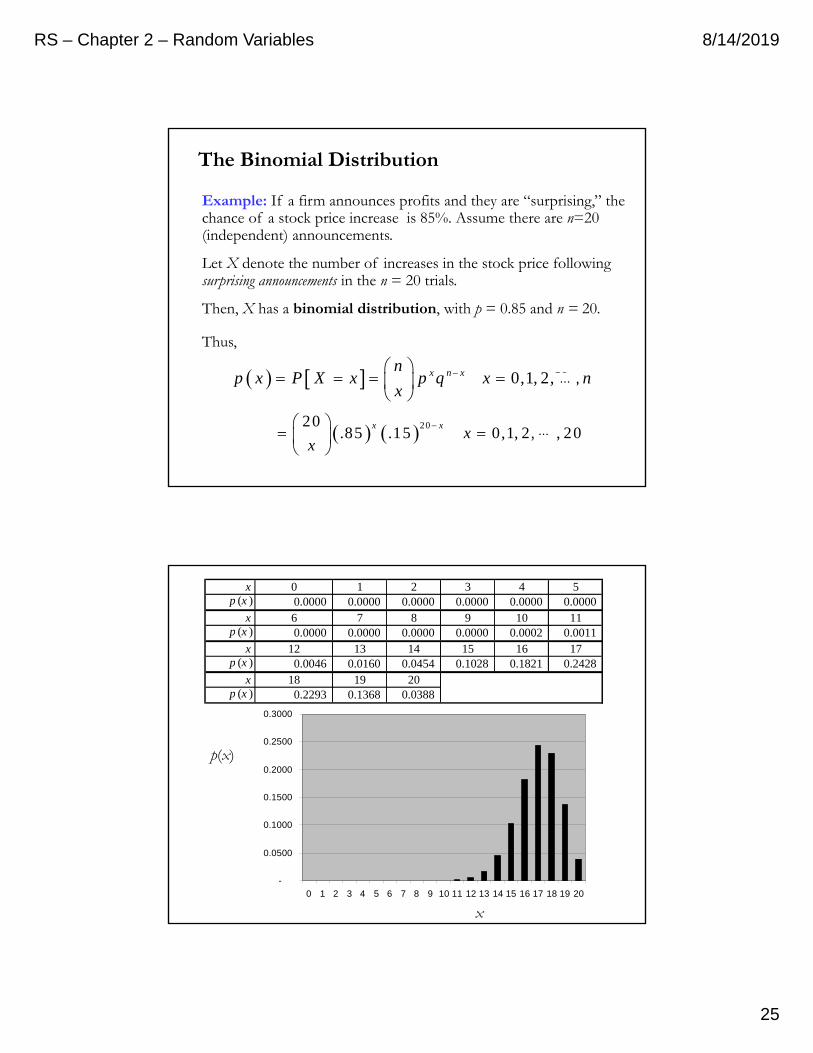
Example: If a firm announces profits and they are “surprising,” the chance of a stock price increase is 85%. Assume there are n=20 (independent) announcements.
Let X denote the number of increases in the stock price following surprising announcements in the n = 20 trials.
Then, X has a binomial distribution, with p = 0.85 and n = 20.
0,1, 2, ,x n xnp x P X x p q x n
x
K
Thus,
2020.85 .15 0,1, 2, , 20
x xx
x
K
The Binomial Distribution
⋯
⋯
-
0.0500
0.1000
0.1500
0.2000
0.2500
0.3000
0 1 2 3 4 5 6 7 8 9 10 11 12 13 14 15 16 17 18 19 20
p(x)
x
x 0 1 2 3 4 5p (x ) 0.0000 0.0000 0.0000 0.0000 0.0000 0.0000
x 6 7 8 9 10 11p (x ) 0.0000 0.0000 0.0000 0.0000 0.0002 0.0011
x 12 13 14 15 16 17p (x ) 0.0046 0.0160 0.0454 0.1028 0.1821 0.2428
x 18 19 20p (x ) 0.2293 0.1368 0.0388
RS – Chapter 2 – Random Variables 8/14/2019
26
The Poisson distribution
Siméon Denis Poisson (1781-1840)
The Poisson distribution
• Suppose events are occurring randomly and uniformly in time.
• The events occur with a known average.
• Let X be the number of events occurring (arrivals) in a fixed period of time (time-interval of given length).
• Typical example: X = Number of crime cases coming before a criminal court per year (original Poisson’s application in 1838.)
• Then, X will have a Poisson distribution with parameter .
• The parameter λ represents the expected number of occurrences in a fixed period of time. The parameter λ is a positive real number.
0,1, 2, 3, 4,!
x
p x e xx
K⋯
RS – Chapter 2 – Random Variables 8/14/2019
27
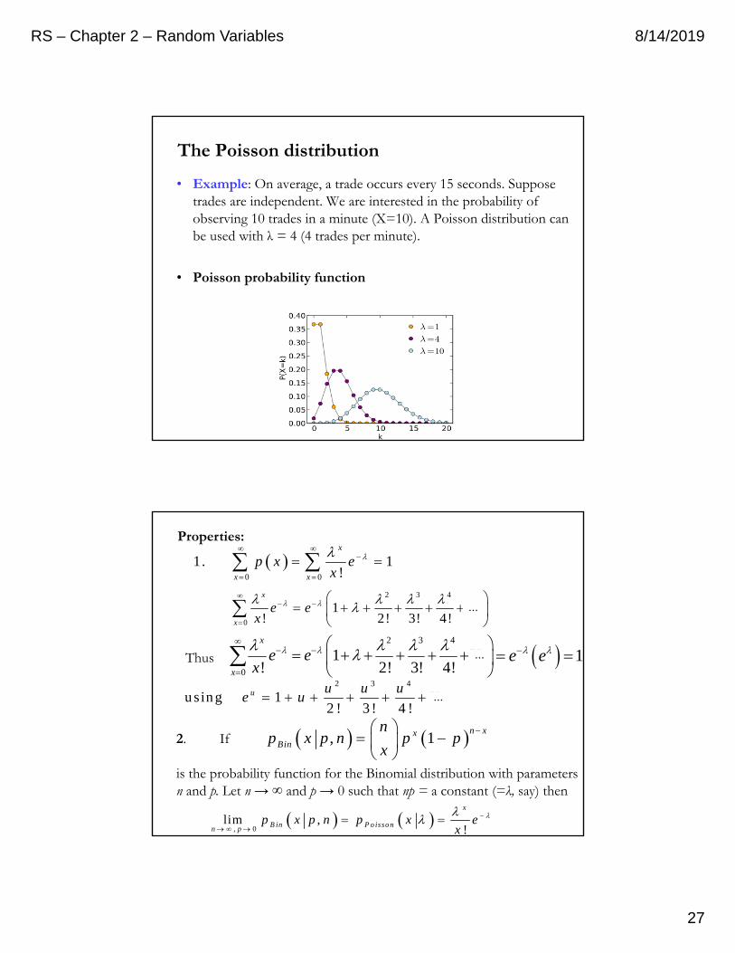
The Poisson distribution
• Example: On average, a trade occurs every 15 seconds. Suppose trades are independent. We are interested in the probability of observing 10 trades in a minute (X=10). A Poisson distribution can be used with λ = 4 (4 trades per minute).
• Poisson probability function
1e e 2 3 4
0
1! 2! 3! 4!
x
x
e ex
K
2 3 4
u sin g 12 ! 3 ! 4 !
u u u ue u K
Thus
2. If
is the probability function for the Binomial distribution with parameters n and p. Let n → ∞ and p → 0 such that np = a constant (=λ, say) then
, 1n xx
Bin
np x p n p p
x
, 0
lim ,!
x
B in P o issonn p
p x p n p x ex
0 0
1. 1!
x
x x
p x ex
2 3 4
0
1! 2! 3! 4!
x
x
e ex
K
Properties:
⋯
⋯
⋯
RS – Chapter 2 – Random Variables 8/14/2019
28
Proof: , 1n xx
Bin
np x p n p p
x
Suppose or np pn
!
, , 1! !
x n x
Bin Bin
np x p n p x n
x n x n n
!
1 1! !
x nx
x
n
x n n x n n
1 11 1
!
x nx n n n x
x n n n n n
L
L
1 11 1 1 1 1
!
x nx x
x n n n n
L
⋯
⋯
⋯
Now lim ,Binn
p x n
1 1lim 1 1 1 1
!
x nx
n
x
x n n n n
L
lim 1!
nx
nx n
Using the classic limit lim 1n
u
n
ue
n
lim , lim 1! !
nx x
Bin Poissonn n
p x n e p xx n x
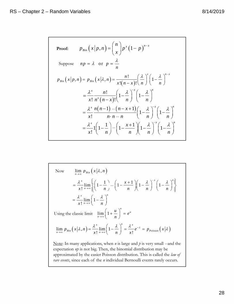
Note: In many applications, when n is large and p is very small --and the expectation np is not big. Then, the binomial distribution may be approximated by the easier Poisson distribution. This is called the law of rare events, since each of the n individual Bernoulli events rarely occurs.
⋯
RS – Chapter 2 – Random Variables 8/14/2019
29
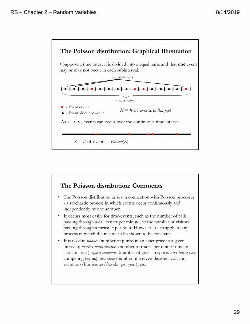
• Suppose a time interval is divided into n equal parts and that one event may or may not occur in each subinterval.
time interval
n subintervals
- Event occurs
- Event does not occur
As n → ∞ , events can occur over the continuous time interval.
X = # of events is Bin(n,p)
X = # of events is Poisson()
The Poisson distribution: Graphical Illustration
The Poisson distribution: Comments
• The Poisson distribution arises in connection with Poisson processes - a stochastic process in which events occur continuously and independently of one another.
• It occurs most easily for time-events; such as the number of calls passing through a call center per minute, or the number of visitors passing through a turnstile per hour. However, it can apply to any process in which the mean can be shown to be constant.
• It is used in finance (number of jumps in an asset price in a given interval); market microstructure (number of trades per unit of time in a stock market); sports economics (number of goals in sports involving two competing teams); insurance (number of a given disaster -volcano eruptions/hurricanes/floods- per year); etc.
RS – Chapter 2 – Random Variables 8/14/2019
30
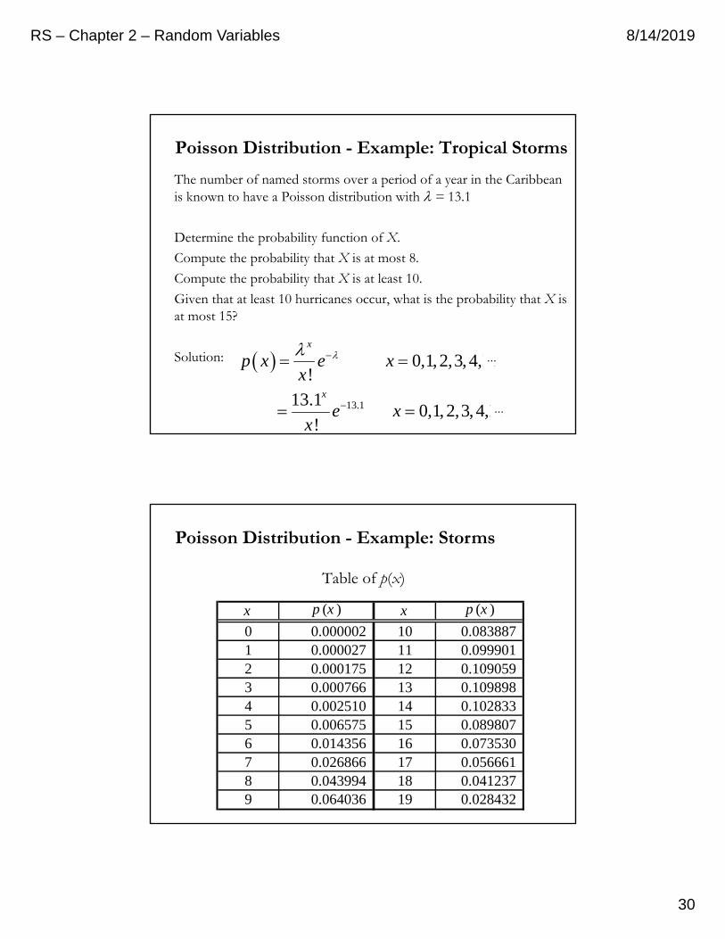
Poisson Distribution - Example: Tropical Storms
The number of named storms over a period of a year in the Caribbean is known to have a Poisson distribution with = 13.1
Determine the probability function of X.
Compute the probability that X is at most 8.
Compute the probability that X is at least 10.
Given that at least 10 hurricanes occur, what is the probability that X is at most 15?
Solution: 0,1, 2,3, 4,!
x
p x e xx
K
13.113.1 0,1, 2,3, 4,
!
x
e xx
K
⋯
⋯
Table of p(x)
x p (x ) x p (x )
0 0.000002 10 0.083887 1 0.000027 11 0.099901 2 0.000175 12 0.109059 3 0.000766 13 0.109898 4 0.002510 14 0.102833 5 0.006575 15 0.089807 6 0.014356 16 0.073530 7 0.026866 17 0.056661 8 0.043994 18 0.041237 9 0.064036 19 0.028432
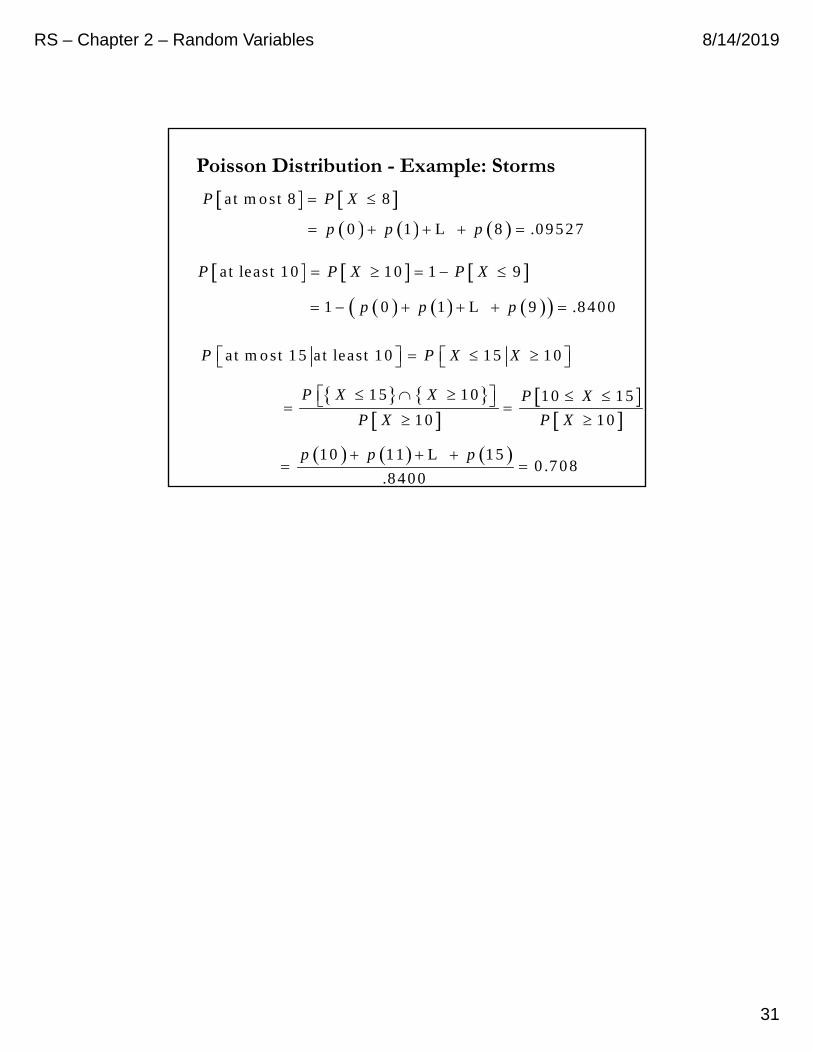
Poisson Distribution - Example: Storms
RS – Chapter 2 – Random Variables 8/14/2019
31
at m o st 8 8P P X
0 1 8 .0 9 5 2 7p p p L
at least 1 0 10 1 9P P X P X
1 0 1 9 .84 00p p p L
at m o st 1 5 at leas t 1 0 1 5 1 0P P X X
1 5 1 0 10 15
1 0 1 0
P X X P X
P X P X
10 11 150 .7 0 8
.8 4 0 0
p p p
L
Poisson Distribution - Example: Storms


![[ T ] Two tiny tigers take two taxis to town `Two `tiny `tigers take `two `taxis to town.](https://static.fdocument.org/doc/165x107/56649d135503460f949e6998/-t-two-tiny-tigers-take-two-taxis-to-town-two-tiny-tigers-take-two-taxis.jpg)