Chapter 19: Proﬁt Maximization Problemd.umn.edu/~watanabe/econ401su09/doc/pmpho.pdf · Intro SPMP...

Intro SPMP Comparative Statics LPMP Factor Demand Returns to Scale Σ

Econ 401 Price Theory

Chapter 19: Profit Maximization Problem

Instructor: Hiroki Watanabe

Summer 2009

1 /49


1 IntroductionOverview

2 Short-Run Profit Maximization ProblemDefinitionsShort-Run Profit Maximization ProblemSolution to Short-Run Profit Maximization ProblemExampleInterpretation

3 Comparative Statics4 Long-Run Profit Maximization Problem

Solution to Long-Run Profit Maximization ProblemTangency Condition & Technical Rate ofSubstitution

5 Factor Demand6 Returns to Scale and Profit Mazimization Problem7 Summary

2 /49


Overview

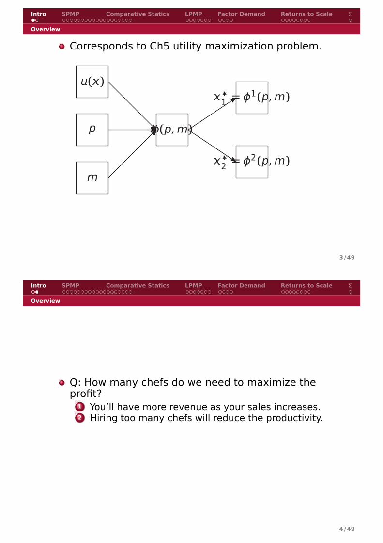
Corresponds to Ch5 utility maximization problem.

ϕ(p,m)

()

p

m

∗1 = ϕ1(p,m)

∗2 = ϕ2(p,m)

Figure:

3 /49


Overview

Q: How many chefs do we need to maximize theprofit?

1 You’ll have more revenue as your sales increases.2 Hiring too many chefs will reduce the productivity.

4 /49







5 /49


Definitions

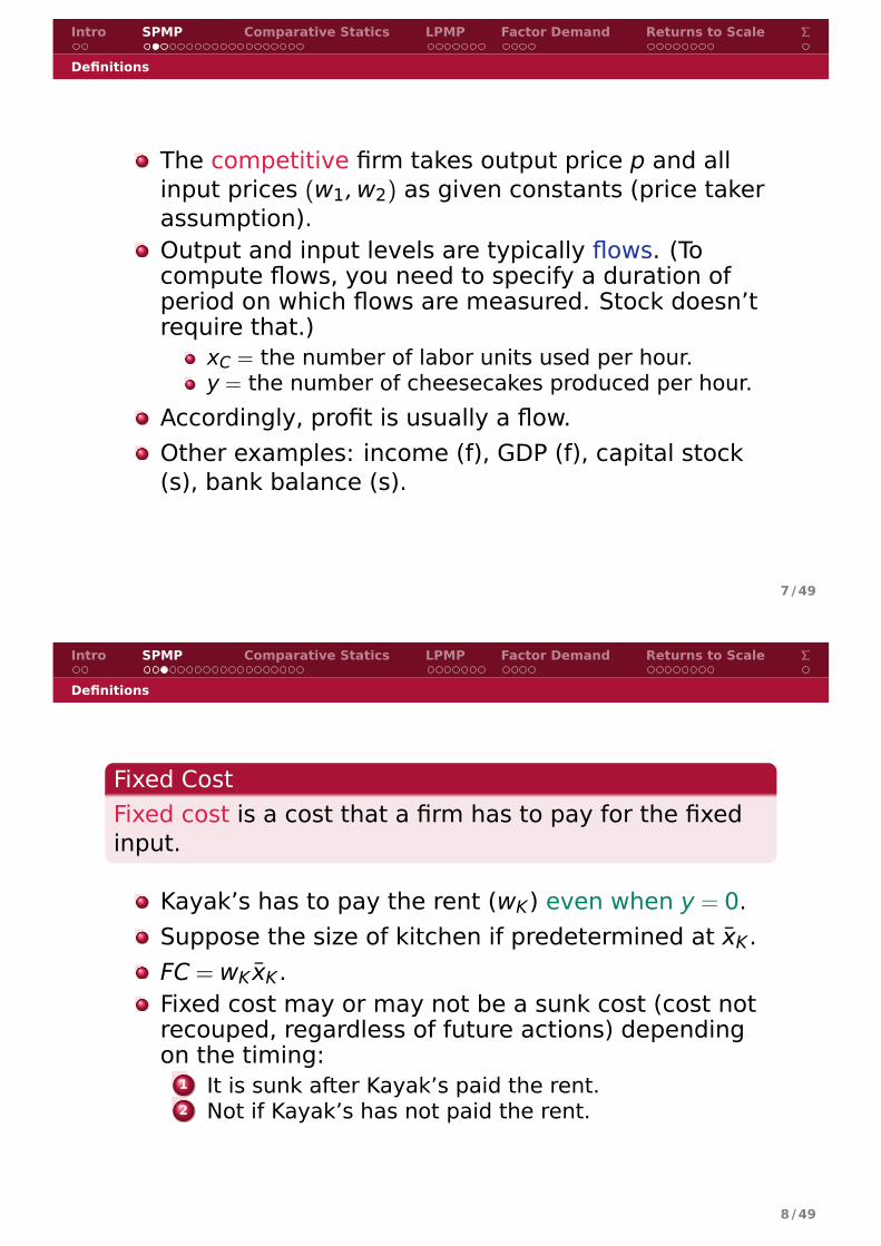
w = (wC,wK) denotes the factor price (unit price ofinputs).The total cost associated with the input bundle(xC,xK) is

TC(xC,xK) = wCxC +wKxK .

The total revenue from y is

TR(y) = py or TR(xC,xK) = pf (xC,xK).

The economic profit generated by the productionplan (xC,xK ,y) is

π(xC,xK) = pf (xC,xK)−wCxC −wKxK .

6 /49


Definitions

The competitive firm takes output price p and allinput prices (w1,w2) as given constants (price takerassumption).Output and input levels are typically flows. (Tocompute flows, you need to specify a duration ofperiod on which flows are measured. Stock doesn’trequire that.)

xC = the number of labor units used per hour.y = the number of cheesecakes produced per hour.

Accordingly, profit is usually a flow.Other examples: income (f), GDP (f), capital stock(s), bank balance (s).

7 /49


Definitions

Fixed CostFixed cost is a cost that a firm has to pay for the fixedinput.

Kayak’s has to pay the rent (wK) even when y = 0.Suppose the size of kitchen if predetermined at x̄K.FC = wK x̄K.Fixed cost may or may not be a sunk cost (cost notrecouped, regardless of future actions) dependingon the timing:

1 It is sunk after Kayak’s paid the rent.2 Not if Kayak’s has not paid the rent.

8 /49


Short-Run Profit Maximization Problem

In the short run, the firm solves the short-run profitmaximization problem (SPMP):

Short-Run Profit Maximization Problem (SPMP)Kayak’s maximizes its short run profit given p, (wC,xK):

maxxC π(xC, x̄K) = pf (xC, x̄K)︸︷︷︸

total revenue

−wCxC −wK x̄K︸︷︷︸

total cost

= pf (xC, x̄K)−wCxC − FC.

9 /49


Solution to Short-Run Profit Maximization Problem

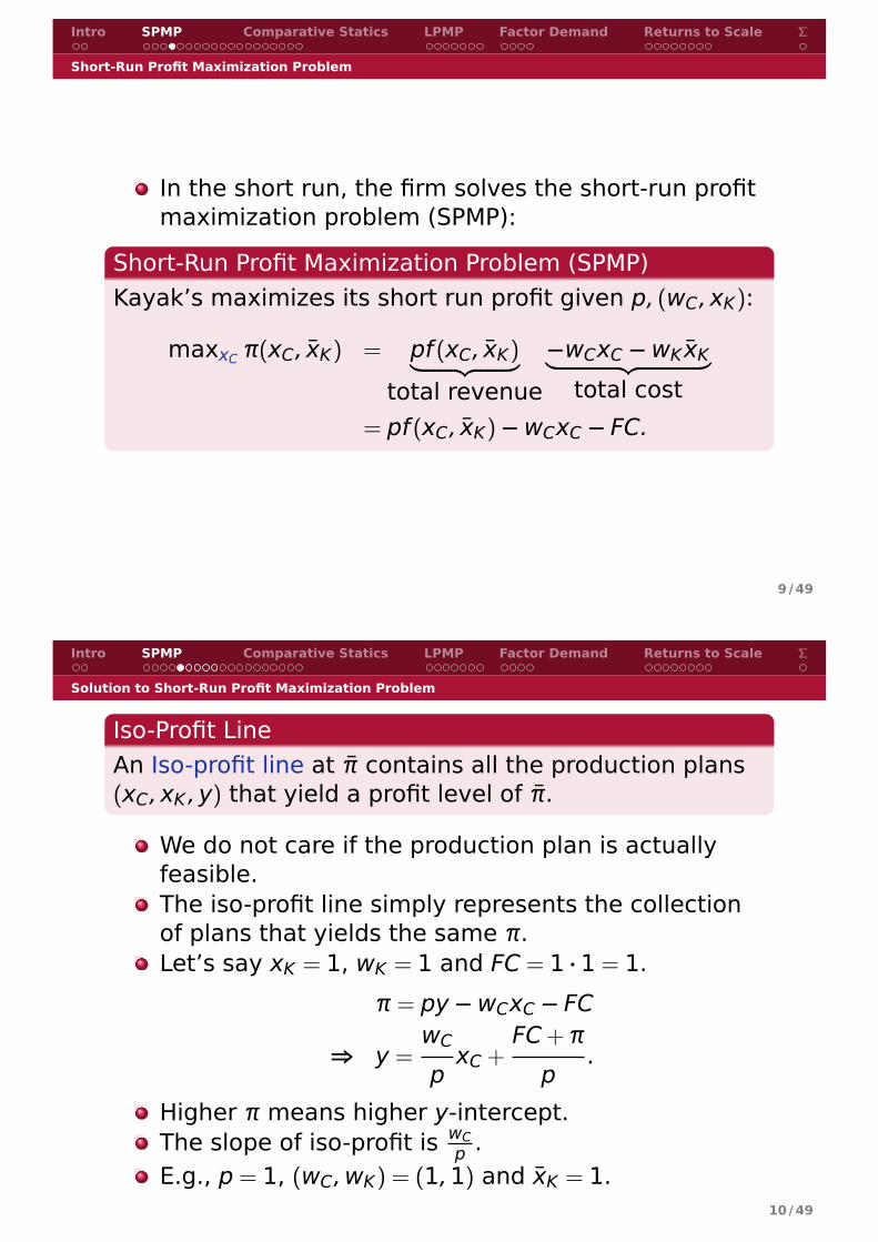
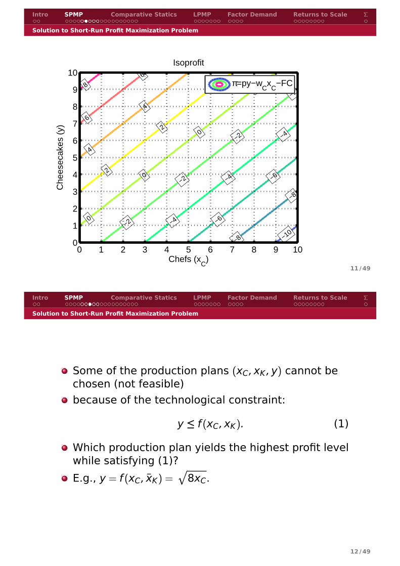
Iso-Profit LineAn Iso-profit line at π̄ contains all the production plans(xC,xK ,y) that yield a profit level of π̄.

We do not care if the production plan is actuallyfeasible.The iso-profit line simply represents the collectionof plans that yields the same π.Let’s say xK = 1, wK = 1 and FC = 1 · 1 = 1.

π = py−wCxC − FC

⇒ y =wC

pxC +

FC+ π

p.

Higher π means higher y-intercept.The slope of iso-profit is wC

p .E.g., p = 1, (wC,wK) = (1,1) and x̄K = 1.

10 /49



−10−8

−8

−6

−6

−4

−4

−4

−2

−2

−2

−20

0

0

0

2

2

2

4

4

6

6

8

Chefs (xC)

Che

esec

akes

(y)

Isoprofit

0 1 2 3 4 5 6 7 8 9 100

1

2

3

4

5

6

7

8

9

10π=py−w

Cx

C−FC

Figure:

11 /49



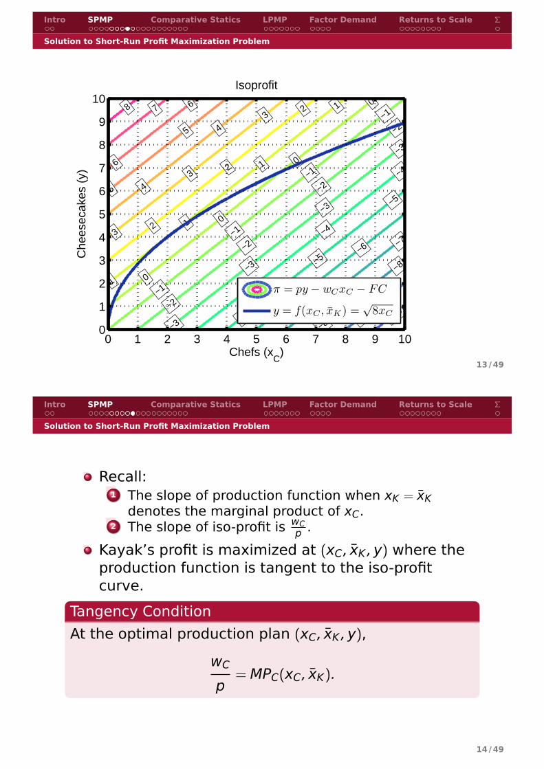
Some of the production plans (xC,xK ,y) cannot bechosen (not feasible)because of the technological constraint:

y ≤ f (xC,xK). (1)

Which production plan yields the highest profit levelwhile satisfying (1)?

E.g., y = f (xC, x̄K) =p

8xC.

12 /49



−10−9

−8

−8

−7

−7

−6

−6

−5

−5

−5

−4

−4

−4

−3

−3

−3

−3

−2

−2

−2

−2

−1

−1

−1

−10

0

0

0

1

1

1

1

2

2

2

3

3

3

4

4

5

5

6

6

78

Chefs (xC)

Che

esec

akes

(y)

Isoprofit

0 1 2 3 4 5 6 7 8 9 100

1

2

3

4

5

6

7

8

9

10

π = py − wCxC − FC

y = f(xC , x̄K) =√

8xC

Figure:

13 /49



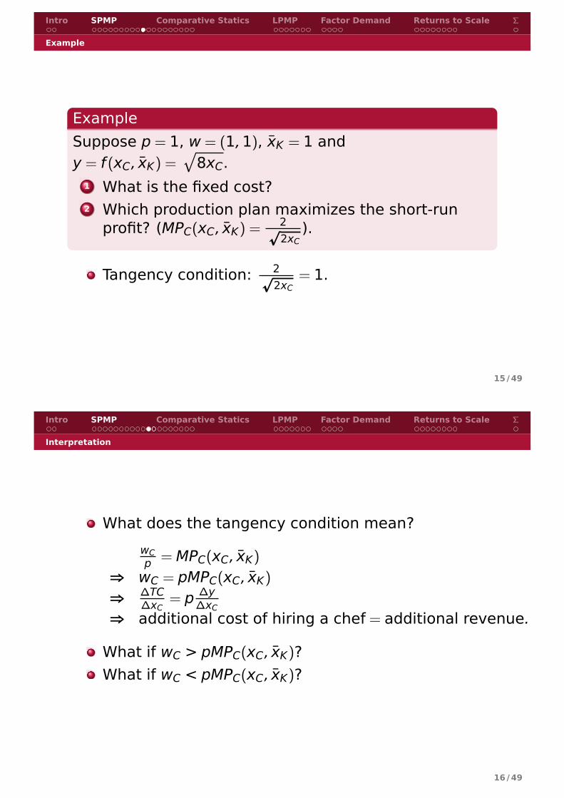
Recall:1 The slope of production function when xK = x̄K

denotes the marginal product of xC.2 The slope of iso-profit is wC

p .

Kayak’s profit is maximized at (xC, x̄K ,y) where theproduction function is tangent to the iso-profitcurve.

Tangency Condition

At the optimal production plan (xC, x̄K ,y),

wC

p= MPC(xC, x̄K).

14 /49


Example

Example

Suppose p = 1, w = (1,1), x̄K = 1 andy = f (xC, x̄K) =

p

8xC.1 What is the fixed cost?2 Which production plan maximizes the short-run

profit? (MPC(xC, x̄K) = 2p2xC

).

Tangency condition: 2p2xC

= 1.

15 /49


Interpretation

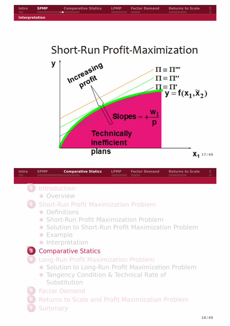
What does the tangency condition mean?

wCp = MPC(xC, x̄K)

⇒ wC = pMPC(xC, x̄K)

⇒ ∆TC∆xC

= p ∆y∆xC

⇒ additional cost of hiring a chef = additional revenue.

What if wC > pMPC(xC, x̄K)?What if wC < pMPC(xC, x̄K)?

16 /49


Interpretation

Figure:

17 /49







18 /49


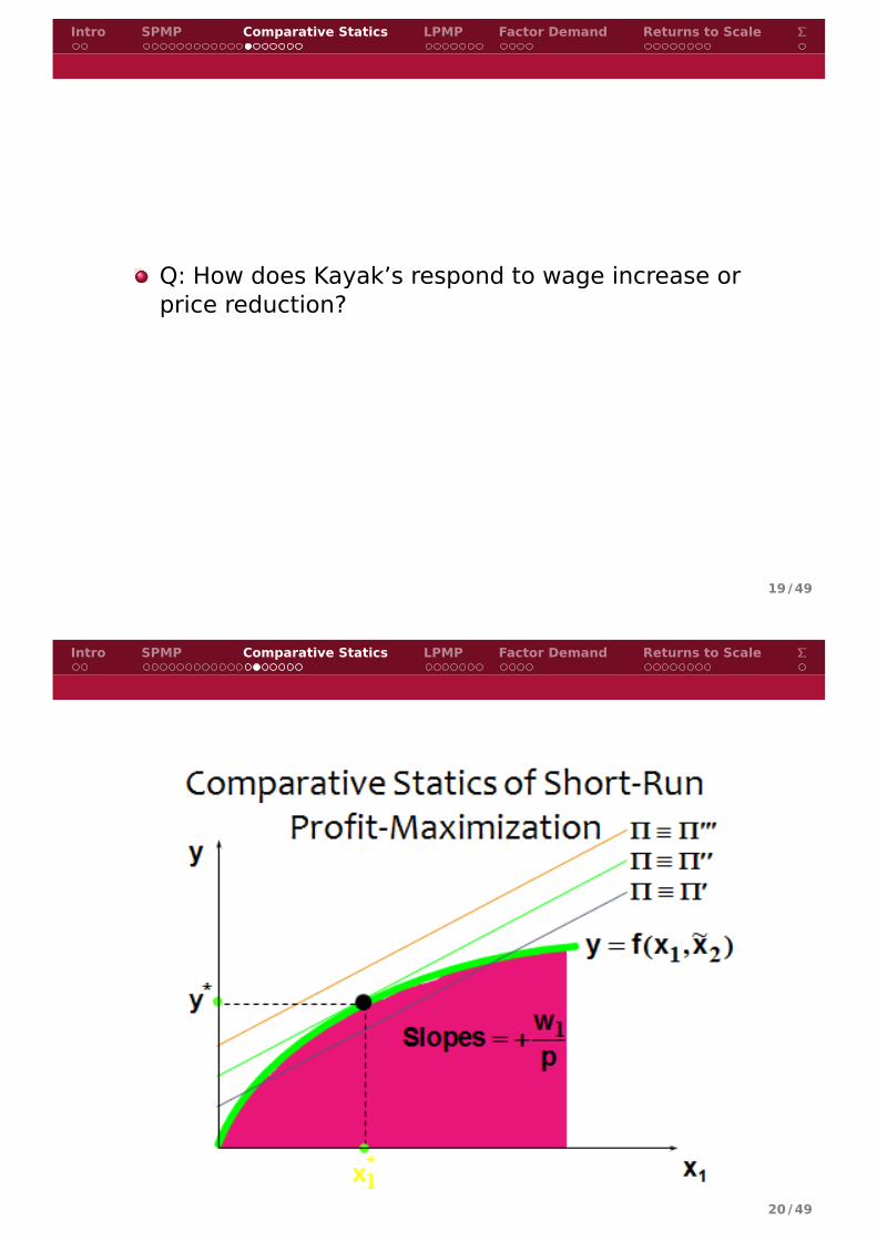
Q: How does Kayak’s respond to wage increase orprice reduction?

19 /49


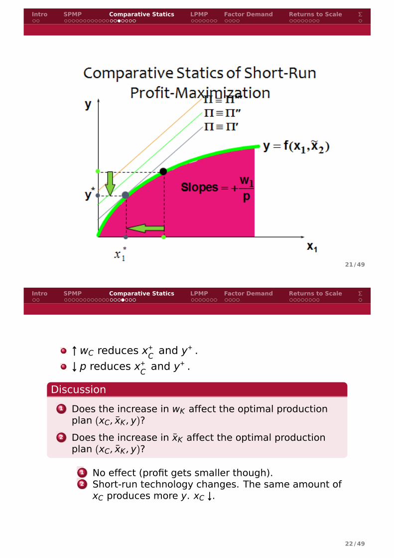
Figure:

20 /49


Figure:

21 /49


↑ wC reduces x+C and y+ .

↓ p reduces x+C and y+ .

Discussion

1 Does the increase in wK affect the optimal productionplan (xC, x̄K ,y)?

2 Does the increase in x̄K affect the optimal productionplan (xC, x̄K ,y)?

1 No effect (profit gets smaller though).2 Short-run technology changes. The same amount of

xC produces more y. xC ↓.

22 /49


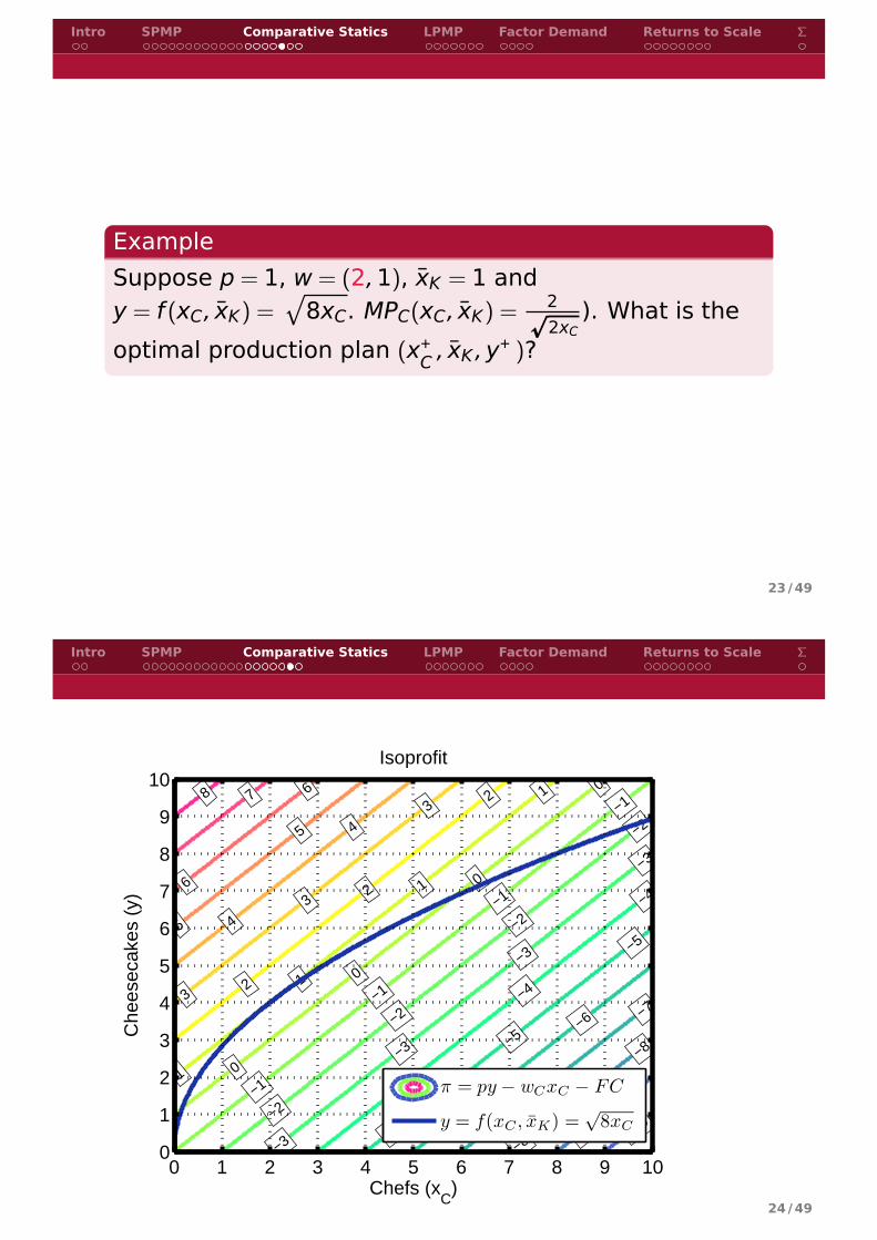
Example

Suppose p = 1, w = (2,1), x̄K = 1 andy = f (xC, x̄K) =

p

8xC. MPC(xC, x̄K) = 2p2xC

). What is the

optimal production plan (x+C , x̄K ,y

+ )?

23 /49


−10−9

−8

−8

−7

−7

−6

−6

−5

−5

−5

−4

−4

−4

−3

−3

−3

−3

−2

−2

−2

−2

−1

−1

−1

−10

0

0

0

1

1

1

1

2

2

2

3

3

3

4

4

5

5

6

6

78

Chefs (xC)

Che

esec

akes

(y)

Isoprofit

0 1 2 3 4 5 6 7 8 9 100

1

2

3

4

5

6

7

8

9

10


y = f(xC , x̄K) =√

8xC

Figure:

24 /49


−20

−15

−15

−10

−10

−10

−5

−5

−5

0

0

0

5

5

Chefs (xC)

Che

esec

akes

(y)

Isoprofit

0 0.5 2 100

2

4

10


y = f(xC , x̄K) =√

8xC

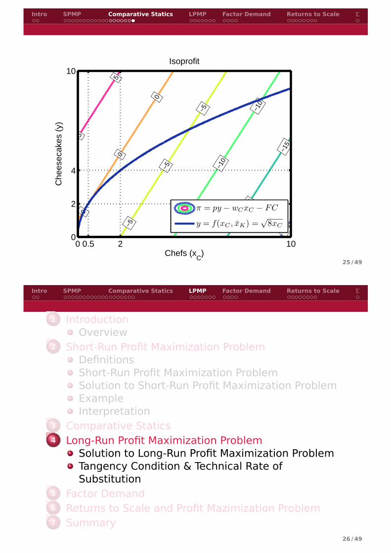
Figure:

25 /49







26 /49


Solution to Long-Run Profit Maximization Problem

Long Run

A long-run is the circumstance in which a firm isunrestricted in its choice of input levels.

Decision-making process in which you can changethe size of the store as well as amount of cheese.x̄K now becomes xK.

27 /49



Long-Run Profit Maximization Problem (LPMP)

Given w and p, in the long run, Kayak’s solves

maxxC,xK

π(xC,xK) = pf (xC,xK)−wCxC −wKxK .

The same condition applies to xK:

wK

p= MPK(x+

C ,xK).

28 /49



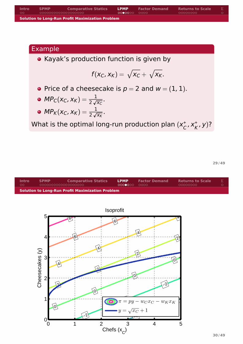
Example

Kayak’s production function is given by

f (xC,xK) =p

xC +p

xK .

Price of a cheesecake is p = 2 and w = (1,1).

MPC(xC,xK) = 12pxC

.

MPK(xC,xK) = 12pxK

.

What is the optimal long-run production plan (x+C ,x

+K ,y)?

29 /49



−4

−4

−2

−2

−2

0

0

0

0

2

2

2

2

4

4

4

46

6

8

Chefs (xC)

Che

esec

akes

(y)

Isoprofit

0 1 2 3 4 50

1

2

3

4

5

π = py − wCxC − wKxK

y =√

xC + 1

Figure:

30 /49



−4

−4

−2

−2

−2

0

0

0

0

2

2

2

2

4

4

4

46

6

8

Size of Kitchen (xK)

Che

esec

akes

(y)

Isoprofit

0 1 2 3 4 50

1

2

3

4

5

π = py − wCxC − wKxK

y = 1 +√

xK

Figure:

31 /49


Tangency Condition & Technical Rate of Substitution

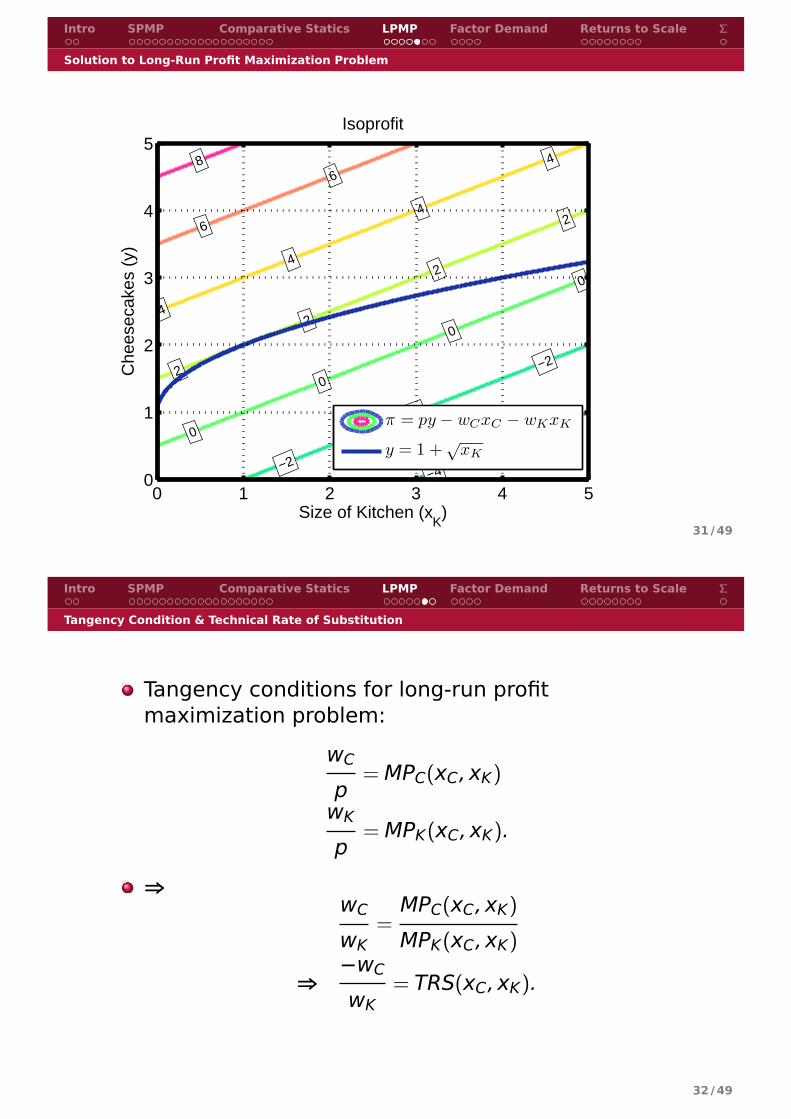
Tangency conditions for long-run profitmaximization problem:

wC

p= MPC(xC,xK)

wK

p= MPK(xC,xK).

⇒wC

wK=MPC(xC,xK)

MPK(xC,xK)

⇒−wC

wK= TRS(xC,xK).

32 /49


Tangency Condition & Technical Rate of Substitution

If Kayak’s fires one chef, they can expand thekitchen area by wC

wK.

If Kayak’s fire one chef, they need to expand thekitchen area by TRS(xC,xK).The factor market’s idea of chef’s worth coincideswith Kayak’s idea of chef’s worth.More details in Ch20: cost minimization problem.

33 /49







34 /49


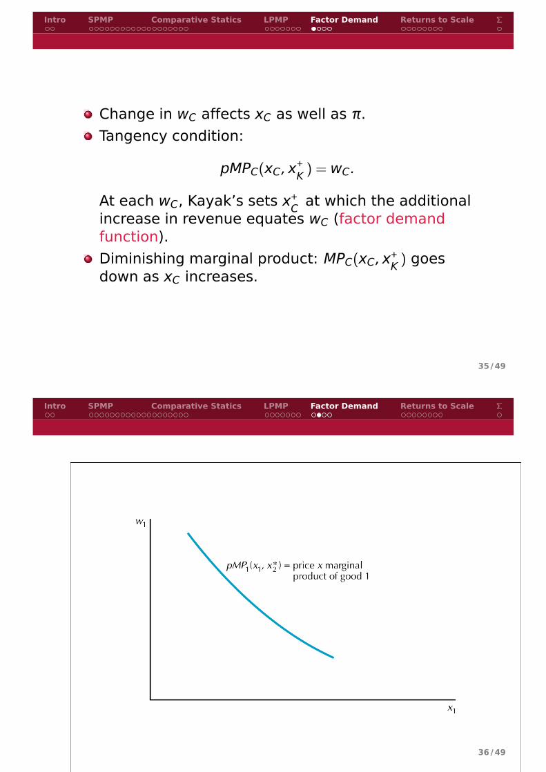
Change in wC affects xC as well as π.Tangency condition:

pMPC(xC,x+K ) = wC.

At each wC, Kayak’s sets x+C at which the additional

increase in revenue equates wC (factor demandfunction).Diminishing marginal product: MPC(xC,x+

K ) goesdown as xC increases.

35 /49


Figure:

36 /49


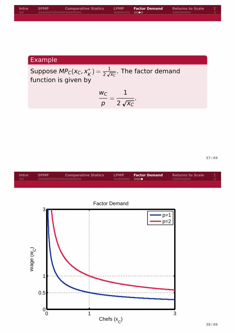
Example

Suppose MPC(xC,x+K ) = 1

2pxC

. The factor demandfunction is given by

wC

p=

1

2pxC.

37 /49


0 1 30

0.5

1

3

Chefs (xC)

Wag

e (w

C)

Factor Demand

p=1p=2

Figure:

38 /49







39 /49


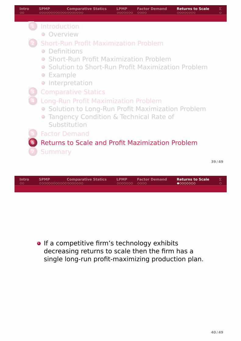
If a competitive firm’s technology exhibitsdecreasing returns to scale then the firm has asingle long-run profit-maximizing production plan.

40 /49


Figure:

41 /49


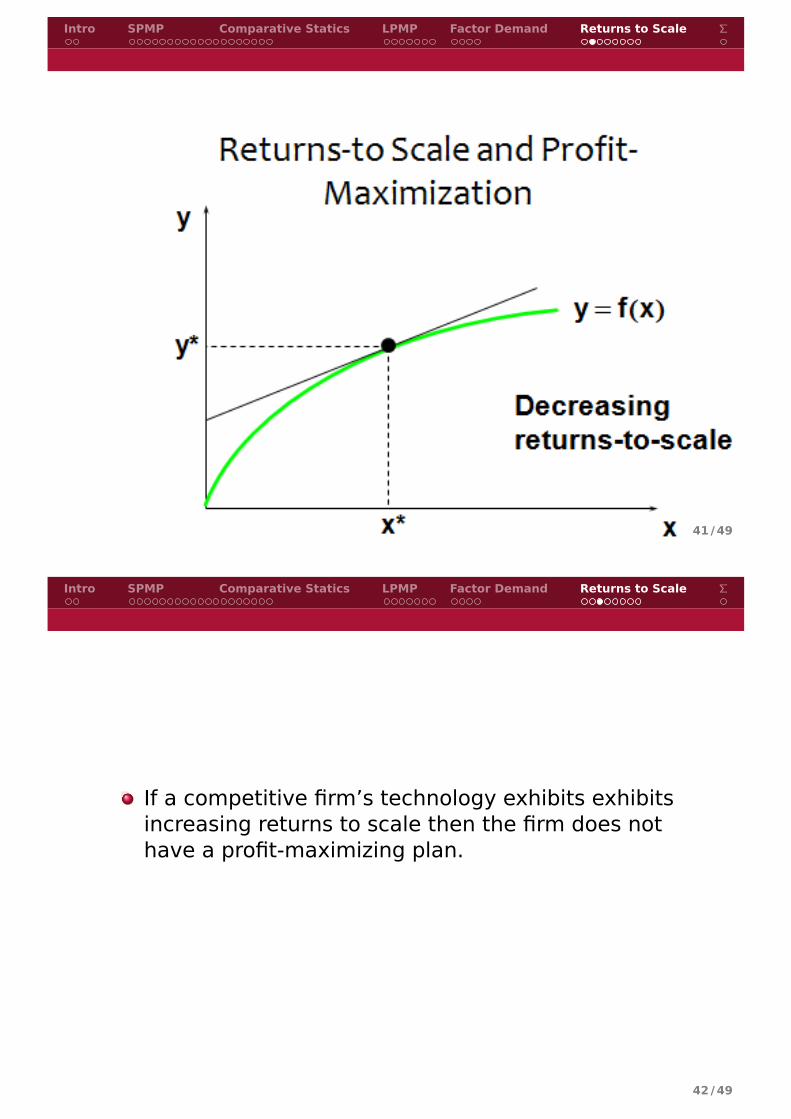
If a competitive firm’s technology exhibits exhibitsincreasing returns to scale then the firm does nothave a profit-maximizing plan.

42 /49


Figure:

43 /49


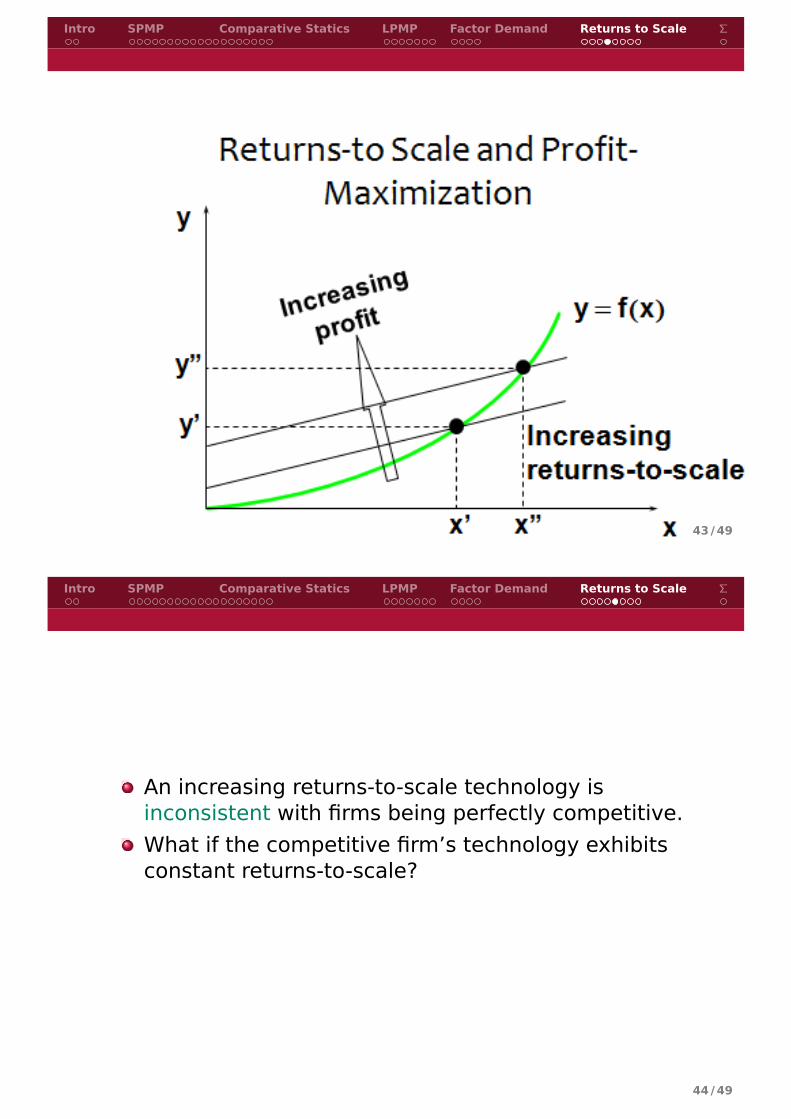
An increasing returns-to-scale technology isinconsistent with firms being perfectly competitive.What if the competitive firm’s technology exhibitsconstant returns-to-scale?

44 /49


Figure:

45 /49


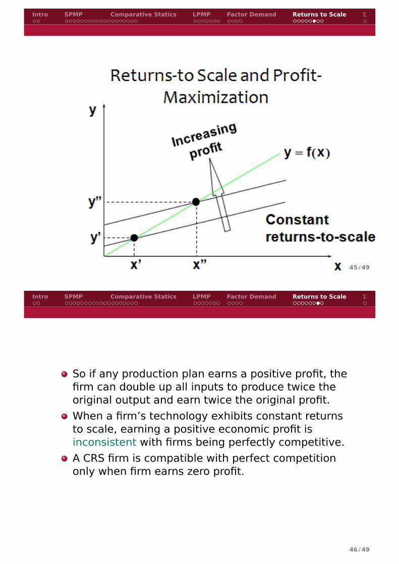
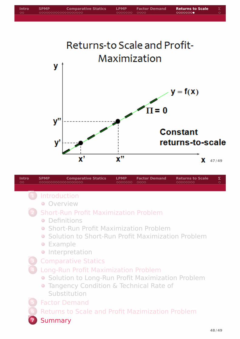
So if any production plan earns a positive profit, thefirm can double up all inputs to produce twice theoriginal output and earn twice the original profit.When a firm’s technology exhibits constant returnsto scale, earning a positive economic profit isinconsistent with firms being perfectly competitive.A CRS firm is compatible with perfect competitiononly when firm earns zero profit.

46 /49


Figure:

47 /49







48 /49


Solving profit maximization problem.Comparative statics.Factor demand.Competitive environment and compatibletechnology.

49 /49

Chapter 19: Proﬁt Maximization Problemd.umn.edu/~watanabe/econ401su09/doc/pmpho.pdf · Intro SPMP...

Documents

Transcript of Chapter 19: Proﬁt Maximization Problemd.umn.edu/~watanabe/econ401su09/doc/pmpho.pdf · Intro SPMP...