Chapter 1

Group Representations

Definition 1.1 A representationα of a groupG in a vector spaceV over k isdefined by a homomorphism

α : G→ GL(V ).

Thedegreeof the representation is the dimension of the vector space:

degα = dimk V.

Remarks:

1. Recall thatGL(V )—the general linear group onV—is the group of invert-ible (or non-singular) linear mapst : V → V .

2. We shall be concerned almost exclusively with representations offinite de-gree, that is, infinite-dimensionalvector spaces; and these will almost al-ways be vector spaces overR or C. Therefore, to avoid repetition, let usagree to use the term ‘representation’ to meanrepresentation of finite de-gree overR or C, unless the contrary is explicitly stated.

Furthermore, in this first Part we shall be concerned almost exclusively withfinitegroups; so let us also agree that the term ‘group’ will meanfinite groupin this Part, unless the contrary is stated.

3. Suppose{e1, . . . , en} is a basis forV . Then each linear mapt : V → V isdefined (with respect to this basis) by ann× n-matrixT . Explicitly,

tej =∑i

Tijei;

424–I 1–1

424–I 1–2

or in terms of coordinates,x1...xn

7→ T

x1...xn

Thus a representation inV can be defined by a homomorphism

α : G→ GL(n, k),

whereGL(n, k) denotes the group of non-singularn×n-matrices overk. Inother words,α is defined by giving matricesA(g) for eachg ∈ G, satisfyingthe conditions

A(gh) = A(g)A(h)

for all g, h ∈ G; and alsoA(e) = I.

4. There is another way of looking at group representations which is almostalways more fruitful than the rather abstract definition we started with.

Recall that a group is said toact on the setX if we have a map

G×X → X : (g, x) 7→ gx

satisfying

(a) (gh)x) = g(hx),

(b) ex = x.

Now supposeX = V is a vector space. Then we can say thatG acts linearlyonV if in addition

(c) g(u+ v) = gu+ gv,

(d) g(ρv) = ρ(gv).

Each representationα of G in V defines a linear action ofG onV , by

gv = α(g)v;

and every such action arises from a representation in this way.

Thus the notions ofrepresentationandlinear actionare completely equiv-alent. We can use whichever we find more convenient in a given case.

424–I 1–3

5. There are two other ways of looking at group representations, completelyequivalent to the definition but expressing slightly different points of view.

Firstly, we may speak of the vector spaceV , with the action ofG on it.as aG-space. For those familiar with category theory, this would be thecategorical approach. Representation theory, from this point of view, is thestudy of the category ofG-spaces andG-maps, where aG-map

t : U → V

from oneG-space to another is a linear map preserving the action ofG, iesatisfying

t(gu) = g(tu) (g ∈ G, u ∈ U).

6. Secondly, and finally, mathematical physicists often speak—strikingly—ofthe vector spaceV carrying the representationα.

Examples:

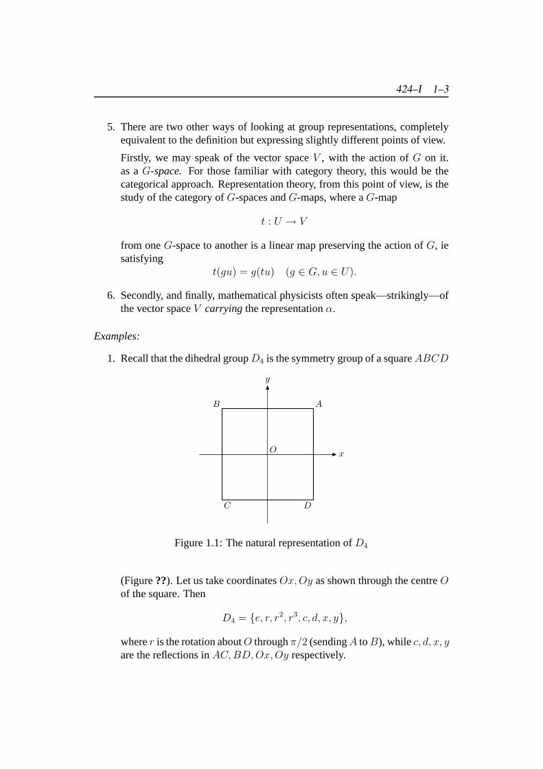
1. Recall that the dihedral groupD4 is the symmetry group of a squareABCD

AB

C D

O x

y

Figure 1.1: The natural representation ofD4

(Figure??). Let us take coordinatesOx,Oy as shown through the centreOof the square. Then

D4 = {e, r, r2, r3, c, d, x, y},

wherer is the rotation aboutO throughπ/2 (sendingA toB), whilec, d, x, yare the reflections inAC,BD,Ox,Oy respectively.

424–I 1–4

By definition a symmetryg ∈ D4 is an isometry of the planeE2 sendingthe square into itself. Evidentlyg must sendO into itself, and so gives riseto a linear map

A(g) : R2 → R2.

The mapg 7→ A(g) ∈ GL(2,R)

defines a 2-dimensional representationρ of D4 overR. We may describethis as thenatural2-dimensional representation ofD4.

(Evidently the symmetry groupG of any bounded subsetS ⊂ En will havea similar ‘natural’ representation inRn.)

The representationρ is given in matrix terms by

e 7→(

1 00 1

), r 7→

(0 −11 0

), r2 7→

(−1 00 −1

), r3 7→

(0 1−1 0

),

c 7→(

0 11 0

), d 7→

(0 −1−1 0

), x 7→

(1 00 −1

), y 7→

(−1 00 1

).

Each group relation is represented in a corresponding matrix equation, eg

cd = r2 =⇒(

0 11 0

)(0 −1−1 0

)=

(−1 00 −1

).

The representationρ is faithful, ie the homomorphism defining it is injec-tive. Thus a relation holds inD4 if and only if the corresponding matrixequation is true. However, representations are not necessarily faithful, andin general the implication is only one way.

Every finite-dimensional representation can be expressed in matrix form inthis way, after choosing a basis for the vector space carrying the representa-tion. However, while such matrix representations are reassuringly concrete,they are impractical except in the lowest dimensions. Better just to keep atthe back of one’s mind that a representationcouldbe expressed in this way.

2. SupposeG acts on the setX:

(g, x) 7→ gx.

LetC(X) = C(X, k)

denote the space of mapsf : X → k.

424–I 1–5

ThenG acts linearly onC(X)—and so defines a representationρ of G—by

gf(x) = f(g−1x).

(We needg−1 rather thang on the right to satisfy the rule

g(hf) = (gh)f.

It is fortunate that the relation

(gh)−1 = h−1g−1

enables us to correct the order reversal. We shall often have occasion totake advantage of this, particularly when dealing—as here—with spaces offunctions.)

Now suppose thatX is finite; say

X = {x1, . . . , xn}.

Thendeg ρ = n = ‖X‖,

the number of elements inX. For the functions

ey(x) =

{1 if x = y,0 otherwise.

(ie the characteristic functions of the 1-point subsets) form a basis forC(X).Also

gex = egx,

since

gey(x) = ey(g−1x)

=

1 if g−1x = y

0 if g−1x 6= y

=

1 if x = gy

0 if x 6= gy

Thusg 7→ P (g)

424–I 1–6

whereP = P (g) is the matrix with entries

Pxy =

{1 if y = gx,0 otherwise.

Notice thatP is apermutation matrix, ie there is just one 1 in each row andcolumn, all other entries being 0. We call a representation that arises fromthe action of a group on a set in this way apermutational representation.

As an illustration, consider the natural action ofS(3) on the set{a, b, c}.This yields a 3-dimensional representationρ of S(3), under which

(abc) 7→

0 1 00 0 11 0 0

(ab) 7→

0 1 01 0 00 0 1

(These two instances actually define the representation, since(abc) and(ab)generateS(3).)

3. A 1-dimensionalrepresentationα of a groupG overk = R orC is just ahomomorphism

α : G→ k×,

wherek× denotes the multiplicative group on the setk \ {0}. For

GL(1, k) = k×,

since we can identify the1× 1-matrix [x] with its single entryx.

We call the 1-dimensional representation defined by the identity homomor-phism

g 7→ 1

(for all g ∈ G) thetrivial representationof G, and denote it by 1.

In a 1-dimensional representation, each group element is represented by anumber. Since these numbers commute, the study of 1-dimensional repre-sentations is much simpler than those of higher dimension.

In general, when investigating the representations of a groupG, we start bydetermining all its 1-dimensional representations.

Recall that two elementsg, h ∈ G are said to beconjugateif

h = xgx−1

424–I 1–7

for some third elementx ∈ G. Supposeα is a 1-dimensional representationof G. Then

α(h) = α(x)α(g)α(x−1)

= α(x)α(g)α(x)−1

= α(g)α(x)α(x)−1

= α(g),

since the numbersα(x), α(g) commute. It follows that a 1-dimensionalrepresentationis constant on each conjugacy class ofG.

Consider the groupS3. This has 3 classes (we shall usually abbreviate ‘con-jugacy class’ toclass):

{1}, {(abc), (acb)}, {(bc), (ca), (ab)}.

Let us writes = (abc), t = (bc).

Then (assumingk = C)

s3 = 1 =⇒ α(s)3 = 1 =⇒ α(s) = 1, ω or ω2,

t2 = 1 =⇒ α(s)2 = 1 =⇒ α(t) = ±1.

Buttst−1 = s2.

It follows thatα(t)α(s)α(t)−1 = α(s)2,

from which we deduce thatα(s) = 1.

It follows that S3 has just two 1-dimensional representations: the trivialrepresentation

1 : g 7→ 1,

and theparity representation

ε : g 7→{

1 if g is even,−1 if g is odd.

4. The corresponding result is true for all the symmetric groupsSn (for n ≥ 2);Sn has just two 1-dimensional representations, the trivial representation 1and the parity representationε.

To see this, let us recall two facts aboutSn.

424–I 1–8

(a) The transpositionsτ = (xy) generateSn, ie each permutationg ∈ Snis expressible (not uniquely) as a product of transpositions

g = τ1 · · · τr.

(b) The transpositions are all conjugate.

(This is a particular case of the general fact that two permutations inSn are conjugate if and only if they are of the samecyclic type, ie theyhave the same number of cycles of each length.)

It follows from (1) that a 1-dimensional representation ofSn is completelydetermined by its values on the transpositions. It follows from (2) that therepresentation is constant on the transpositions. Finally, since each trans-positionτ satisfiesτ 2 = 1 it follows that this constant value is±1. Thusthere can only be two 1-dimensional representations ofSn; the first takes thevalue 1 on the transpositions, and so is 1 everywhere; the second takes thevalue -1 on the transpositions, and takes the value(−1)r on the permutation

g = τ1 · · · τr.

ThusSn has just two 1-dimensional representations; the trivial representa-tion 1 and the parity representationε.

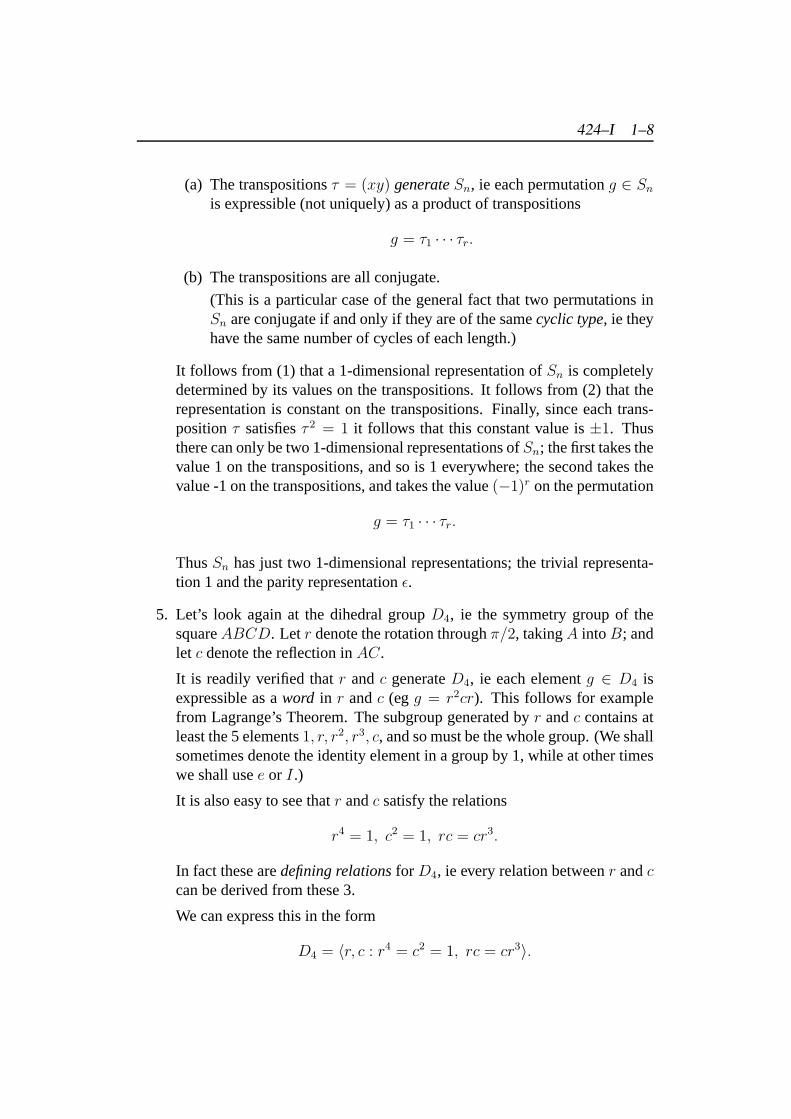
5. Let’s look again at the dihedral groupD4, ie the symmetry group of thesquareABCD. Let r denote the rotation throughπ/2, takingA intoB; andlet c denote the reflection inAC.

It is readily verified thatr andc generateD4, ie each elementg ∈ D4 isexpressible as aword in r andc (eg g = r2cr). This follows for examplefrom Lagrange’s Theorem. The subgroup generated byr andc contains atleast the 5 elements1, r, r2, r3, c, and so must be the whole group. (We shallsometimes denote the identity element in a group by 1, while at other timeswe shall usee or I.)

It is also easy to see thatr andc satisfy the relations

r4 = 1, c2 = 1, rc = cr3.

In fact these aredefining relationsfor D4, ie every relation betweenr andccan be derived from these 3.

We can express this in the form

D4 = 〈r, c : r4 = c2 = 1, rc = cr3〉.

424–I 1–9

Now supposeα is a 1-dimensional representation ofD4. Then we musthave

α(r)4 = α(c)2 = 1, α(r)α(c) = α(c)α(r)3.

From the last relationα(r)2 = 1.

Thus there are just 4 possibilities

α(r) = ±1, α(c) = ±1.

It is readily verified that all 4 of these satisfy the 3 defining relations forsandt. It follows that each defines a homomorphism

α : D4 → k×.

We conclude thatD4 has just 4 1-dimensional representations.

6. We look now at some examples from chemistry and physics. It should beemphasized, firstly that the theory is completely independent of these ex-amples, which can safely be ignored; and secondly, thatwe are not on oathwhen speaking of physics. It would be inappropriate to delve too deeplyhere into the physical basis for the examples we give.

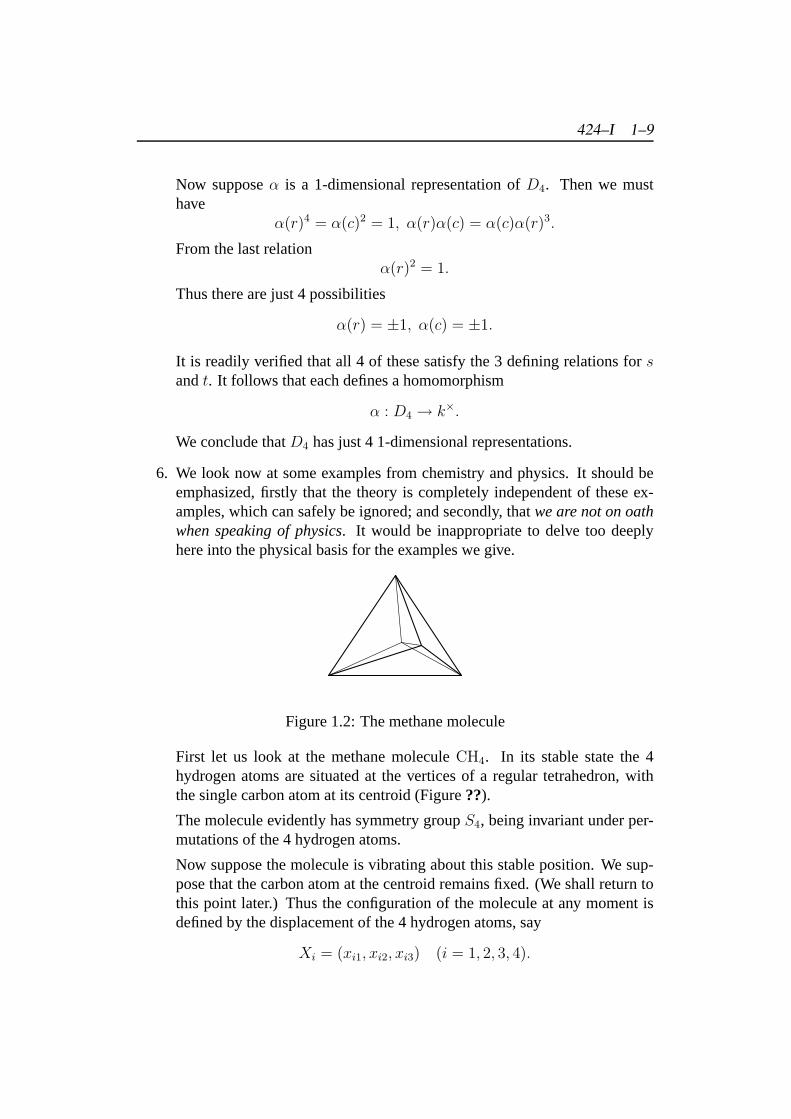
Figure 1.2: The methane molecule

First let us look at the methane moleculeCH4. In its stable state the 4hydrogen atoms are situated at the vertices of a regular tetrahedron, withthe single carbon atom at its centroid (Figure??).

The molecule evidently has symmetry groupS4, being invariant under per-mutations of the 4 hydrogen atoms.

Now suppose the molecule is vibrating about this stable position. We sup-pose that the carbon atom at the centroid remains fixed. (We shall return tothis point later.) Thus the configuration of the molecule at any moment isdefined by the displacement of the 4 hydrogen atoms, say

Xi = (xi1, xi2, xi3) (i = 1, 2, 3, 4).

424–I 1–10

Since the centroid remains fixed,∑i

xij = 0 (j = 1, 2, 3).

This reduces the original 12 degrees of freedom to 9.

Now let us assume further that theangular momentum also remains 0, iethe molecule is not slowly rotating. This imposes a further 3 conditions onthexij, leaving 6 degrees of freedom for the 12 ‘coordinates’xij. Mathe-matically, the coordinates are constrained to lie in a 6-dimensional space.In other words we can find 6 ‘generalized coordinates’q1, . . . , q6 — chosenso thatq1 = q2 = · · · = q6 = 0 at the point of equilibrium — such that eachof thexij is expressible in terms of theqk:

xij = xij(q1, . . . , q6).

The motion of the molecule is governed by the Euler-Lagrange equations

d

dt

(∂K

∂qk

)= −∂V

∂qk

whereK is the kinetic energy of the system, andV its potential energy.(These equations were developed for precisely this purpose, to express themotion of a system whose configuration is defined by generalized coordi-nates.)

The kinetic energy of the system is given in terms of the massm of thehydrogen atom by

K =1

2m∑i,j

x2ij

On substituting

xij =∂xij∂q1

q1 + · · ·+ ∂xij∂q6

q6,

we see thatK = K(q1, . . . , q6),

whereK is a positive-definite quadratic form. Although the coefficientsof this quadratic form are actually functions ofq1, . . . , q6, we may supposethem constant since we are dealing with small vibrations.

The potential energy of the system, which we may take to have minimalvalue 0 at the stable position, is given to second order by some positive-definite quadratic formQ in theqk:

V = Q(q1, . . . , q6) + . . . .

424–I 1–11

While we could explicitly choose the coordinatesqk, and determine the ki-netic energyK, the potential energy formQ evidently depends on the forcesholding the molecule together. Fortunately, we can say a great deal about thevibrational modes of the molecule without knowing anything about theseforces.

Since these two forms are positive-definite, we can simultaneously diag-onalize them, ie we can find new generalized coordinatesz1, . . . , z6 suchthat

K = z21 + · · ·+ z2

6 ,

V = ω21z

21 + · · ·+ ω2

6z26 .

The Euler-Lagrange equations now give

zi = −ω2i zi (i = 1, . . . , 6).

Thus the motion is made up of 6 independent harmonic oscillations, withfrequenciesω1, . . . , ω6.

As usual when studying harmonic or wave motion, life is easier if we allowcomplex solutions (of which the ‘real’ solutions will be the real part). Eachharmonic oscillation then has 1 degree of freedom:

zj = Cjeiωjt.

The set of all solutions of these equations (ie all possible vibrations of thesystem) thus forms a 6-dimensionalsolution-spaceV .

So far we have made no use of theS4-symmetry of theCH4 molecule. Butnow we see that this symmetry group acts on the solution spaceV , whichthus carries a representation,ρ say, ofS4. Explicitly, supposeπ ∈ S4 isa permutation of the 4 H atoms. This permutation is ‘implemented’ bya unique spatial isometryΠ. (For example, the permutation(123)(4) iseffected by rotation through1/3 of a revolution about the axis joining the Catom to the 4th H atom.)

But now if we apply this isometryΠ to any vibrationv(t) we obtain a newvibration Πv(t). In this way the permutationπ acts on the solution-spaceV .

In general,the symmetry groupG of the physical configuration will act onthe solution-spaceV .

The fundamental result in the representation theory of a finite groupG (aswe shall establish) is that every representationρ of G splits into parts, each

424–I 1–12

corresponding to a ‘simple’ representation ofG. Each finite group has a fi-nite number of such simple representations, which thus serve as the ‘atoms’out of which every representation ofG is constructed. (There is a closeanalogy with the Fundamental Theorem of Arithmetic, that every naturalnumber is uniquely expressible as a product of primes.)

The groupS4 (as we shall find) has 5 simple representations, of dimensions1, 1, 2, 3, 3. Our 6-dimensional representation must be the ‘sum’ of some ofthese.

It is not hard to see that there is just one 1-dimensional mode (up to a scalarmultiple) corresponding to a ‘pulsing’ of the molecule in which the 4 Hatoms move in and out (in ‘sync’) along the axes joining them to the cen-tral C atom. (Recall thatS4 has just two 1-dimensional representations: thetrivial representation, under which each permutation leaves everything un-changed, and the parity representation, in which even permutations leavethings unchanged, while odd permutations reverse them. In our case, the4 atoms must move in the same way under the trivial representation, whiletheir motion is reversed under an odd permutation. The latter is impossible.For by considering the odd permutation(12)(3)(4) we deduce that the firstatom is moving out while the second moves in; while under the action ofthe even permutation(12)(34) the first and second atoms must move in andout together.)

We conclude (not rigorously, it should be emphasized!) that

ρ = 1 + α + β

where1 denotes the trivial representation ofS4,α is the unique 2-dimensionalrepresentation, andβ is one of the two 3-dimensional representations.

Thus without any real work we’ve deduced quite a lot about the vibrationsof CH4.

Each of these 3 modes has a distinct frequency. To see that, note that oursystem — and in fact any similar non-relativistic system — has atime sym-metrycorresponding to the additive groupR. For if (zj(t) : 1 ≤ j ≤ 6) isone solution then(zj(t+ c)) is also a solution for any constantc ∈ R.

The simple representations ofR are just the 1-dimensional representations

t 7→ eiωt.

(We shall see that the simple representations of anabeliangroup are always1-dimensional.) In effect, Fourier analysis — the splitting of a function

424–I 1–13

or motion into parts corresponding to different frequencies — is just therepresentation theory ofR.

The actions ofS4 andR on the solution space commute, giving a represen-tation of the product groupS4 × R.

As we shall see, the simple representations of a product groupG×H arisefrom simple representations ofG andH: ρ = σ× τ . In the present case wemust have

ρ = 1× E(ω1) + α× E(ω2) + β × E(ω3),

whereω1, ω2, ω3 are the frequencies of the 3 modes.

If the symmetry is slightly broken, eg by placing the vibrating molecule ina magnetic field, these ‘degenerate’ frequencies will split, so that 6 frequen-cies will be seen:ω′1, ω

′2, ω

′′2 , ω

′3, ω

′′3 , ω

′′′3 , where egω′2 andω′′2 are close toω.

This is the origin of ‘multiple lines’ in spectroscopy.

The concept ofbroken symmetryhas become one of the corner-stones ofmathematical physics. In ‘grand unified theories’ distinct particles are seenas identical (like our 4 H atoms) under some large symmetry group, whoseaction is ‘broken’ in our actual universe.

7. Vibrations of a circular drum. [?]. Consider a circular elastic membrane.The motion of the membrane is determined by the function

z(x, y, t) (x2 + y2 ≤ r2)

wherez is the height of the point of the drum at position(x, y).

It is not hard to establish that under small vibrations this function will satisfythe wave equation

T

(∂2z

∂x2+∂2z

∂y2

)= ρ

∂2z

∂t2,

whereT is the tension of the membrane andρ its mass per unit area. Thismay be written (

∂2z

∂x2+∂2z

∂y2

)=

1

c2

∂2z

∂t2,

wherec = (T/ρ)1/2 is thespeedof the wave motion.

The configuration hasO(2) symmetry, whereO(2) is the group of 2-dimensionalisometries leaving the centreO fixed, consisting of the rotations aboutOand the reflections in lines throughO.

424–I 1–14

Although this group is not finite, it iscompact. As we shall see, the repre-sentation theory of compact groups is essentially identical to the finite the-ory; the main difference being that a compact group has a countable infinityof simple representations.

For example, the groupO(2) has the trivial representation 1, and an infinityof representationsR(1), R(2), . . . , each of dimension 2.

The circular drum has corresponding modesM(0),M(1),M(2), . . . , eachwith its characteristic frequency. As in our last example, after taking timesymmetry into account, the solution-space carries a representationρ of theproduct groupO(2)× R, which splits into

1× E(ω0) +R(1)× E(ω1) +R(2)× E(ω2) + · · · .

8. In the last example but one, we considered the 4 hydrogen atoms in themethane molecule as particles, or solid balls. But now let us consider asingle hydrogen atom, consisting of an electron moving in the field of amassive central proton.

According to classical non-relativistic quantum mechanics [?], the state ofthe electron (and so of the atom) is determined by awave functionψ(x, y, z, t),whose evolution is determined bySchrodinger’s equation

i~∂ψ

∂t= Hψ.

HereH is thehamiltonian operator, given by

Hψ = − ~2

2m∇2ψ + V (r)ψ,

wherem is the mass of the electron,V (t) is its potential energy,~ isPlanck’s constant, and

∇2ψ =∂2ψ

∂x2+∂2ψ

∂y2+∂2ψ

∂z2.

Thus Schrodinger’s equation reads, in full,

i~∂ψ

∂t= − ~

2

2m

(∂2ψ

∂x2+∂2ψ

∂y2+∂2ψ

∂z2

)− e2

rψ.

The essential point is that this is alinear differential equation, whose solu-tions therefore form a vector space, thesolution-space.

424–I 1–15

We regard the central proton as fixed atO. (A more accurate account mighttakeO to be the centre of mass of the system.) The system is invariant underthe orthogonal groupO(3), consisting of all isometries — that is, distance-preserving transformations — which leaveO fixed. Thus the solution spacecarries a representation of the compact groupO(3).

This group is a product-group:

O(3) = SO(3)× C2,

whereC2 = {I, J} (J denoting reflection inO), while SO(3) is the sub-group of orientation-preserving isometries. In fact, each such isometry is arotation about some axis, soSO(3) is group of rotations in 3 dimensions.

The rotation groupSO(3) has simple representationsD0, D1, D2, . . . ofdimensions1, 3, 5, . . . . To each of these corresponds amodeof the hy-drogen atom, with a particular frequencyω and corresponding energy levelE = ~ω.

These energy levels are seen in the spectroscope, although the spectral linesof hydrogen actually correspond todifferencesbetween energy levels, sincethey arise from photons given off when the energy level changes.

This idea — considering the space of atomic wave functions as a repre-sentation ofSO(3) gave the first explanation of the periodic table of theelements, proposed many years before by Mendeleev on purely empiricalgrounds [?].

The discussion above ignores thespinof the electron. In fact representationtheory hints strongly at the existence of spin, since the ‘double-covering’SU(2) of SO(3) adds the ‘spin representations’D1/2, D3/2, . . . of dimen-sions2, 4, . . . to the sequence above, as we shall see.

Finally, it is worth noting that quantum theory (as also electrodynamics) arelinear theories, where the Principle of Superposition rules. Thus the appli-cation of representation theory is exact, and not an approximation restrictedto small vibrations, as in classical mechanical systems like the methanemolecule, or the drum.

9. The classification of elementary particles. [?]. Consider an elementaryparticleE, eg an electron, in relativistic quantum theory. The possible statesof E again correspond to the points of a vector spaceV . More precisely,they correspond to the points of theprojective spaceP (V ) formed by therays, or 1-dimensional subspaces, ofV . For the wave functionsψ andρψcorrespond to the same state ofE.

424–I 1–16

The state spaceV is now acted on by thePoincare groupE(1, 3) formed bythe isometries of Minkowski space-time. It follows thatV carries a repre-sentation ofE(1, 3).

Each elementary particle corresponds to a simple representation of thePoincare groupE(1, 3). This group is not compact. It is however aLiegroup; and — as we shall see — a different approach to representation the-ory, based onLie algebras, allows much of the theory to be extended to thiscase.

A last remark. One might suppose, from its reliance on linearity, that rep-resentation theory would have no role to play in curved space-time. Butthat is far from true. Even if the underlying topological space is curved, thevector and tensorfieldson such a space preserve their linear structure. (Soone can, for example, superpose vector fields on a sphere.) Thus represen-tation theory can still be applied; and in fact, the so-calledgauge theoriesintroduced in the search for a unified ‘theory of everything’ are of preciselythis kind.

Bibliography

[1] C. A. Coulson.Waves. Oliver and Boyd, 1955.

[2] Richard Feynman.Lecture Notes on Physics III. Addison-Wesley, 196.

[3] D. J. Simms.Lie Groups and Quantum Mechanics. Springer, 1968.

[4] Hermann Weyl. The Theory of Groups and Quantum Mechanics. Dover,1950.

424–I 1–17

BIBLIOGRAPHY 424–I 1–18

Exercises

All representations are overC, unless the contrary is stated.

In Exercises 01–11 determine all 1-dimensional representations of the given group.

1 ∗ C2 2 ∗∗ C3 3 ∗∗ Cn 4 ∗∗ D2 5 ∗∗ D3

6 ∗∗∗ Dn 7 ∗∗∗ Q8 8 ∗∗∗ A4 9 ∗∗∗∗ An 10∗∗ Z11∗∗∗∗ D∞ = 〈r, s : s2 = 1, rsr = s〉

SupposeG is a group; and supposeg, h ∈ G. The element[g, h] = ghg−1h−1 iscalled thecommutatorof g andh. The subgroupG′ ≡ [G,G] is generated by allcommutators inG is called the commutator subgroup, orderived groupof G.

12∗∗∗ Show thatG′ lies in the kernel of any 1-dimensional representationρ of G,ie ρ(g) acts trivially if g ∈ G′.13 ∗∗∗ Show thatG′ is a normal subgroup ofG, and thatG/G′ is abelian. Showmoreover that ifK is a normal subgroup ofG thenG/K is abelian if and only ifG′ ⊂ K. [In other words,G′ is the smallest normal subgroup such thatG/G′ isabelian.)

14 ∗∗ Show that the 1-dimensional representations ofG form an abelian groupG∗ under multiplication. [Nb: this notationG∗ is normally only used whenG isabelian.]

15∗∗ Show thatC∗n ∼= Cn.

16∗∗∗ Show that for any 2 groupsG,H

(G×H)∗ = G∗ ×H∗.

17 ∗∗∗∗ By using the Structure Theorem on Finite Abelian Groups (stating thateach such group is expressible as a product of cyclic groups) or otherwise, showthat

A∗ ∼= A

for any finite abelian groupA.

18∗∗ SupposeΘ : G→ H is a homomorphism of groups. Then each representa-tion α of H defines a representationΘα of G.

19∗∗∗ Show that the 1-dimensional representations ofG and ofG/G′ are in one-one correspondence.

In Exercises 20–24 determine the derived groupG′ of the given groupG.

20∗∗∗ Cn 21∗∗∗∗ Dn 22∗∗ Z 23∗∗∗∗ D∞24∗∗∗ Q8 25∗∗∗ Sn 26∗∗∗ A4 27∗∗∗∗ An

Chapter 2

Equivalent Representations

Every mathematical theory starts from some notion of equivalence—an agree-ment not to distinguish between objects that ‘look the same’ in some sense.

Definition 2.1 Supposeα, β are two representations ofG in the vector spacesU, V overk. We say thatα andβ areequivalent, and we writeα = β, if U andVare isomorphicG-spaces.

In other words, we can find a linear map

t : U → V

which preserves the action ofG, ie

t(gu) = g(tu) for all g ∈ G, u ∈ U.

Remarks:

1. Supposeα andβ are given in matrix form:

α : g 7→ A(g), β : g 7→ B(g).

If α = β, thenU andV are isomorphic, and so in particulardimα = dim β,ie the matricesA(g) andB(g) are of the same size.

Suppose the linear mapt : U → V is given by the matrixP . Then theconditiont(gu) = g(tu) gives

B(g) = PA(g)P−1

for eachg ∈ G. This is the condition in matrix terms for two representationsto be equivalent.

424–I 2–1

424–I 2–2

2. Recall that twon × n matricesS, T are said to besimilar if there exists anon-singular (invertible) matrixP such that

T = PSP−1.

A necessary condition for this is thatA,B have the same eigenvalues. Forthe characteristic equations of two similar matrices are identical:

det(PSP−1 − λI

)= detP det(S − λI) detP−1

= det(S − λI).

3. In general this condition is necessary but not sufficient. For example, thematrices (

1 00 1

),

(1 10 1

)have the same eigenvalues 1,1, but are not similar. (No matrix is similar tothe identity matrixI exceptI itself.)

However, there is one important case, or particular relevance to us, wherethe converse is true. Let us recall a result from linear algebra.

An n × n complex matrixA is diagonalisable if and only if it satisfies aseparable polynomial equation, ie one without repeated roots.

It is easy to see that ifA is diagonalisable then it satisfies a separable equa-tion. For if

A ∼

λ1

...λ1

λ2

...

thenA satisfies the separable equation

m(x) ≡ (x− λ1)(x− λ2) · · · = 0.

The converse is less obvious. SupposeA satisfies the polynomial equation

p(x) ≡ (x− λ1) · · · (x− λr) = 0

with λ1, . . . , λr distinct. Consider the expression of1/p(x) as a sum ofpartial fractions:

1

p(x)=

a1

x− λ1

+ · · ·+ arx− λr

.

424–I 2–3

Multiplying across,

1 = a1Q1(x) + · · ·+ arQr(x),

where

Qi(x) =∏j 6=i

(x− λj) =p(x)

x− λi.

Substitutingx = A,

I = a1Q1(A) + · · ·+ arQr(A).

Applying each side to the vectorv ∈ V ,

v = a1Q1(A)v + · · ·+ arQr(A)v

= v1 + · · ·+ vr,

say. The vectorvi is an eigenvector ofA with eigenvalueλi, since

(A− λi)vi = aip(A)v = 0.

Thus every vector is expressible as a sum of eigenvectors. In other wordsthe eigenvectors ofA span the space.

But that is precisely the condition forA to be diagonalisable. For we canfind a basis forV consisting of eigenvectors, and with respect to this basisA will be diagonal.

4. It is important to note that while each matrixA(g) is diagonalisablesepa-rately, we cannot in general diagonalise all theA(g) simultaneously. Thatwould imply that theA(g) commuted, which is certainly not the case ingeneral.

5. However, we can show thatif A1, A2, . . . is a set of commuting matricesthen they can be diagonalised simultaneously if and only if they can bediagonalised separately.

To see this, supposeλ is an eigenvalue ofA1. Let

E = {v : A1v = λv}

be the corresponding eigenspace. ThenE is stable under all theAi, since

v ∈ E =⇒ A1(Aiv) = AiA1v = λAiv =⇒ Aiv ∈ E.

424–I 2–4

Thus we have reduced the problem to the simultaneous diagonalisation ofthe restrictions ofA2, A3, . . . to the eigenspaces ofA1. A simple inductiveargument on the degree of theAi yields the result.

In our case, this means that we can diagonalise some (or all) of our repre-sentation matrices

A(g1), A(g2), . . .

if and only it these matrices commute.

This is perhaps best seen as a result on the representations of abelian groups,which we shall meet later.

6. To summarise, two representationsα, β are certainlynotequivalent ifA(g), B(g)have different eigenvalues for someg ∈ G.

Suppose to the contrary thatA(g), B(g) have the same eigenvalues for allg ∈ G. Then as we have seen

A(g) ∼ B(g)

for all g, ieB(g) = P (g)A(g)P (g)−1

for some invertible matrixP (g).

Remarkably, we shall see that if this is so for allg ∈ G, then in factα andβ are equivalent. In other words, if such a matrixP (g) exists for allg thenwe can find a matrixP independent ofg such that

B(g) = PA(g)P−1

for all g ∈ G.

7. SupposeA ∼ B, ieB = PAP−1.

We can interpret this as meaning thatA andB represent the same lineartransformation, under the change of basis defined byP .

Thus we can think of two equivalent representations as being, if effect, thesamerepresentation looked at from two points of view, that is, taking twodifferent bases for the representation-space.

Example:Let us look again at the natural 2-dimensional real representationρ ofthe symmetry groupD4 of the squareABCD. Recall that when we took coordi-nates with respect to axesOx,Oy bisectingDA, AB, ρ took the matrix form

s 7→(

0 −11 0

)c 7→

(0 11 0

),

424–I 2–5

wheres is the rotation through a right-angle (sendingA toB), andc is the reflec-tion inAC.

Now suppose we choose instead the axesOA,OB. Then we obtain the equiv-alent representation

s 7→(

0 −11 0

)c 7→

(1 00 −1

).

We observe thatc has the same eigenvalues,±1, in both cases.Since we have identified equivalent representations, it makes sense to ask for

all the representations of a given groupG of dimensiond, say. What we have todo in such a case is to give a list ofd-dimensional representations, prove that everyd-dimensional representation is equivalent to one of them, and show also that notwo of the representations are equivalent.

It isn’t at all obvious that the number of such representations is finite, evenafter we have identified equivalent representations. We shall see later that this isso:a finite groupG has only a finite number of representations of each dimension.

Example:Let us find all the 2-dimensional representations overC of

S3 = 〈s, t : s3 = t2 = 1, st = ts2〉,

that is, all 2-dimensional representationsup to equivalence.Supposeα is a representation ofS(3) in the 2-dimensional vector spaceV .

Consider the eigenvectors ofs. There are 2 possibilities:

1. s has an eigenvectore with eigenvalueλ 6= 1. Sinces3 = 1, it follows thatλ3 = 1, ieλ = ω or ω2.

Now letf = te. Then

sf = ste = ts2e = λ2te = λ2f.

Thusf is also an eigenvector ofs, although now with eigenvectorλ2.

Sincee andf are eigenvectors corresponding to different eigenvalues, theymust be linearly independent, and therefore span (and in fact form a basisfor) V :

V = 〈e, f〉.

Sincese = λe, sf = λ2f , we see thats is represented with respect to thisbasis by the matrix

s 7→(λ 00 λ2

).

424–I 2–6

On the other hand,te = f, tf = t2e = e, and so

t 7→(

0 11 0

).

The 2 casesλ = ω, ω2 give the representations

α : s 7→(ω 00 ω2

), t 7→

(0 11 0

);

β : s 7→(ω2 00 ω

), t 7→

(0 11 0

);

In fact these 2 representations are equivalent,

α = β,

since one is got from the other by the swapping the basis elements:e, f 7→f, e.

2. The alternative possibility is that both eigenvalues ofs are equal to1. Inthat case, sinces is diagonalisable, it follows that

s 7→ I =

(1 00 1

)

with respect to some basis. But then it follows that this remains the casewith respect to every basis:s is always represented by the matrixI.

In particular,s is always diagonal. So if we diagonalisec—as we know wecan—then we will simultaneously diagonalises andc, and so too all theelements ofD4.

Suppose

s 7→(

1 00 1

), t 7→

(λ 00 µ

).

Then it is evident thats 7→ 1, t 7→ λ

ands 7→ 1, t 7→ µ

will define two 1-dimensional representations ofS3. But we know theserepresentations; there are just 2 of them. In combination, these will give 4

424–I 2–7

2-dimensional representations ofS3. However, two of these will be equiv-alent. The 1-dimensional representations 1 andε give the 2-dimensionalrepresentation

s 7→(

1 00 1

), t 7→

(1 00 −1

).

(Later we shall denote this representation by1 + ε, and call it thesumof 1andε.)

On the other hand,ε and 1 in the opposite order give the representation

s 7→(

1 00 1

), t 7→

(−1 00 1

).

This is equivalent to the previous case, one being taken into the other by thechange of coordinates(x, y) 7→ (y, x). (In other words,ε+ 1 = 1 + ε.)

We see from this that we obtain just3 2-dimensional representations ofS3

in this way (in the notation above they will be1 + 1, 1 + ε andε+ ε).

Adding the single 2-dimensional representation from the first case, we con-clude thatS3 has just 4 2-dimensional representations.

It is easy to see that no 2 of these 4 representations are equivalent, by consid-ering the eigenvalues ofs andc in the 4 cases.

424–I 2–8

Exercises

All representations are overC, unless the contrary is stated.

In Exercises 01–15 determine all 2-dimensional representations (up to equiva-lence) of the given group.

1 ∗∗ C2 2 ∗∗ C3 3 ∗∗ Cn 4 ∗∗∗ D2 5 ∗∗∗ D4

6 ∗∗∗ D5 7 ∗∗∗∗ Dn 8 ∗∗∗ S3 9 ∗∗∗∗ S4 10∗∗∗∗∗ Sn11∗∗∗∗ A4 12∗∗∗∗∗ An 13∗∗∗ Q8 14∗∗ Z 15∗∗∗∗ D∞

16 ∗∗∗ Show that a real matrixA ∈ Mat(n,R) is diagonalisable overR if andonly if its minimal polynomial has distinct roots, all of which are real.

17∗∗∗ Show that a rational matrixA ∈Mat(n,Q) is diagonalisable overQ if andonly if its minimal polynomial has distinct roots, all of which are rational.

18∗∗∗∗ If 2 real matricesA,B ∈Mat(n,R) are similar overC, are they necessar-ily similar overR, ie can we find a matrixP ∈ GL(n,R) such thatB = PAP−1?

19 ∗∗∗∗ If 2 rational matricesA,B ∈ Mat(n,Q) are similar overC, are theynecessarily similar overQ?

20 ∗∗∗∗∗ If 2 integral matricesA,B ∈ Mat(n,Z) are similar overC, are theynecessarily similar overZ, ie can we find an integral matrixP ∈ GL(n,Z) withintegral inverse, such thatB = PAP−1?

The matrixA ∈Mat(n, k) is said to besemisimpleif its minimal polynomial hasdistinct roots. It is said to benilpotentif Ar = 0 for somer > 0.

21 ∗∗∗ Show that a matrixA ∈ Mat(n, k) cannot be both semisimple and nilpo-tent, unlessA = 0.

22∗∗∗ Show that a polynomialp(x) has distinct roots if and only if

gcd (p(x), p′(x)) = 1.

23 ∗∗∗∗ Show that every matrixA ∈ Mat(n,C) is uniquely expressible in theform

A = S +N,

whereS is semisimple,N is nilpotent, and

SN = NS.

(We callS andN the semisimple and nilpotent parts ofA.)

24∗∗∗∗ Show thatS andN are expressible as polynomials inA.

424–I 2–9

25 ∗∗∗∗ Suppose the matrixB ∈ Mat(n,C) commutes with all matrices thatcommute withA, ie

AX = XA =⇒ BX = XB.

Show thatB is expressible as a polynomial inA.

Chapter 3

Simple Representations

Definition 3.1 The representationα ofG in the vector spaceV overk is said tobesimpleif no proper subspace ofV is stable underG.

In other words,α is simple if it has the following property: ifU is a subspaceof V such that

g ∈ G, u ∈ U =⇒ gu ∈ U

then eitherU = 0 orU = V .

Proposition 3.1 1. A 1-dimensional representation overk is necessarily sim-ple.

2. If α is a simple representation ofG overk then

dimα ≤ ‖G‖.

Proof I (1) is evident since a 1-dimensional space has no proper subspaces, stableor otherwise.

For (2), supposeα is a simple representation ofG in V . Take anyv 6= 0 in V ,and consider the set of alltransformsgv of V . LetU be the subspace spanned bythese:

U = 〈gv : g ∈ G〉.

Eachg ∈ G permutes the transforms ofv, since

g(hv) = (gh)v.

It follows thatg sendsU into itself. ThusU is stable underG. Sinceα is simple,by hypothesis,

V = U.

424–I 3–1

424–I 3–2

But sinceU is spanned by the‖G‖ transforms ofv,

dimV = dimU ≤ ‖G‖.

J

Remark:This result can be greatly improved, as we shall see. Ifk = C—the caseof greatest interest to us—then we shall prove that

dimα ≤ ‖G‖12

for any simple representationα.We may as well announce now the full result. SupposeG is a finite group.

Then we shall show (in due course) that

1. The number of simple representations ofG overC is equal to the numbersof conjugacy classes inG;

2. The dimensions of the simple representationsσ1, . . . , σs ofG overC satisfythe relation

dim2 σ1 + · · ·+ dim2 σs = ‖G‖.

3. The dimension each simple representationσi divides the order of the group:

dimσi | ‖G‖.

Of course we cannot use these results in any proof; and in fact we will noteven use them in examples. But at least they provide a useful check on our work.

Examples:

1. The first stage in studying the representation theory of a groupG is to de-termine the simple representations ofG.

Let us agree henceforth to adopt the convention that if the scalar fieldk isnot explicitly mentioned, then we may take it thatk = C.

We normally start our search for simple representations by listing the 1-dimensional representations. In this case we know thatS3 has just 2 1-dimensional representations, the trivial representation 1, and the parity rep-resentationε.

Now suppose thatα is a simple representation ofS3 of dimension> 1.Recall that

S3 = 〈s, t : s3 = t2 = 1, /; st = ts2〉,

wheres = (abc), /; t = (ab).

424–I 3–3

Let e be an eigenvector ofs. Thus

se = λe,

wheres3 = 1 =⇒ λ3 = 1 =⇒ λ = 1, ω, or ω2.

Letf = te.

Thensf = ste = ts2e = λ2te = λ2f.

Thusf is also an eigenvector ofs, but with eigenvalueλ2.

Now consider the subspace

U = 〈e, f〉

spanned bye andf . ThenU is stable unders andt, and so underS3. For

se = λe, sf = λ2f, te = f, tf = t2e = e.

It follows, sinceα is simple, that

V = U.

So we have shown, in particular, that the simple representations ofS3 canonly have dimension 1 or 2.

Let us consider the 3 possible values forλ:

(a) λ = ω. In this case the representation takes the matrix form

s 7→(ω 00 ω2

), t 7→

(0 11 0

).

(b) λ = ω2. In this case the representation takes the matrix form

s 7→(ω2 00 ω

), t 7→

(0 11 0

).

But this is the same representation as the first,since the coordinateswap(x, y) 7→ (y, x) takes one into the other.

424–I 3–4

(c) λ = 1. In this case

se = e, sf = f =⇒ sv = v for all v ∈ V .

In other wordss acts as the identity onV . It follows thats is repre-sented by the matrixI with respect toanybasis ofV .

(More generally, isg ∈ G is represented by a scalar multipleρI ofthe identity with respect to one basis, then it is represented byρI withrespect to every basis; because

P (ρI)P−1 = ρI,

if you like.)

So in this case we can turn tot, leavings to ‘look after itself’. Letebe an eigenvector oft. Then the 1-dimensional space

U = 〈e〉

is stable underS3, since

se = e, /; te = ±e.

Sinceα is simple, it follows thatV = U , ie V is 1-dimensional, con-trary to hypothesis.

We conclude thatS3 has just 3 simple representations

1, ε andα,

of dimensions 1, 1 and 2, given by

1 : s 7→ 1, /; t 7→ 1

ε : s 7→ 1, /; t 7→ −1

α : s 7→(ω 00 ω2

), t 7→

(0 11 0

).

2. Now let us determine the simple representations (overC) of the quaterniongroup

Q8 = 〈s, t : s4 = 1, s2 = t2, st = ts3〉,

wheres = i, /; t = j. (It is best to forget at this point that one of theelements ofQ8 is called−1, and anotheri, since otherwise we shall fallinto endless confusion.)

424–I 3–5

We know thatQ8 has four 1-dimensional representations, given by

s 7→ ±1, t 7→ ±1.

Supposeα is a simple representation ofQ8 in V , of dimension> 1. Let ebe an eigenvector ofs:

se = λe,

wheres4 = 1 =⇒ λ = ±1,±i.

Lette = f.

Thensf = ste = ts3e = λ3te = λ3f.

So as in the previous example,f is also an eigenvector ofs, but with eigen-valueλ3.

Again, as in that example, the subspace

U = 〈e, f〉

is stable underQ8, since

se = λe, sf = λ3f, te = f, tf = t2e = s2e = λ2e.

So V = U , and{e, f} is a basis forV . With respect to this basis ourrepresentation takes the form

s 7→(λ 00 λ3

), t 7→

(0 λ2

1 0

),

whereλ = ±1,±i.If λ = 1 this representation is not simple, since the 1-dimensional subspace

〈(1, 1)〉

is stable underQ8. (This is the same argument as before. Every vector is aneigenvector ofs, so we can find a simultaneous eigenvector by taking anyeigenvector oft.)

The same argument holds ifλ = −1, sinces is represented by−I withrespect to one basis, and so also with respect to any basis. Again, the sub-space

〈(1, 1)〉

424–I 3–6

is stable underQ8, contradicting our assumption that the representation issimple, and of dimension> 1.

We are left with the casesλ = ±i. In fact these are equivalent. For ifλ = −i, thenf is ans-eigenvector with eigenvalueλ3 = i. So takingf inplace ofe we may assume thatλ = i.

We conclude thatQ8 has just 5 simple representations, of dimensions 1,1,1,1,2,given by

1 : s 7→ 1, /; t 7→ 1

µ : s 7→ 1, /; t 7→ −1

ν : s 7→ −1, /; t 7→ 1

ρ : s 7→ −1, /; t 7→ −1

α : s 7→(i 00 −i

), t 7→

(0 −11 0

).

We end by considering a very important case:abelian(or commutative) groups.

Proposition 3.2 A simple representation of a finite abelian group overC is nec-essarily 1-dimensional.

Proof I Supposea ∈ A. Letλ be an eigenvalue ofa, and let

E(λ) = {v ∈ V : av = λv}.

be the corresponding eigenspace.ThenE(λ) is stable underA. For

b ∈ A, v ∈ E(λ) =⇒ a(bv) = (ab)v = (ba)v = b(av) = b(λv) = λ(bv)

=⇒ bv ∈ E(λ).

ThusE(λ) is stable underb, and so underA. But sinceV is simple, by hypothesis,it follows that

E(λ) = V.

In other wordsa acts as a scalar multiple of the identity:

a = λI.

It follows thateverysubspace ofV is stable undera. Since that is true for eacha ∈ A, we conclude that every subspace ofV is stable underA. Therefore, sinceα is simple,V has no proper subspaces. But that is only true ifdimV = 1. J

424–I 3–7

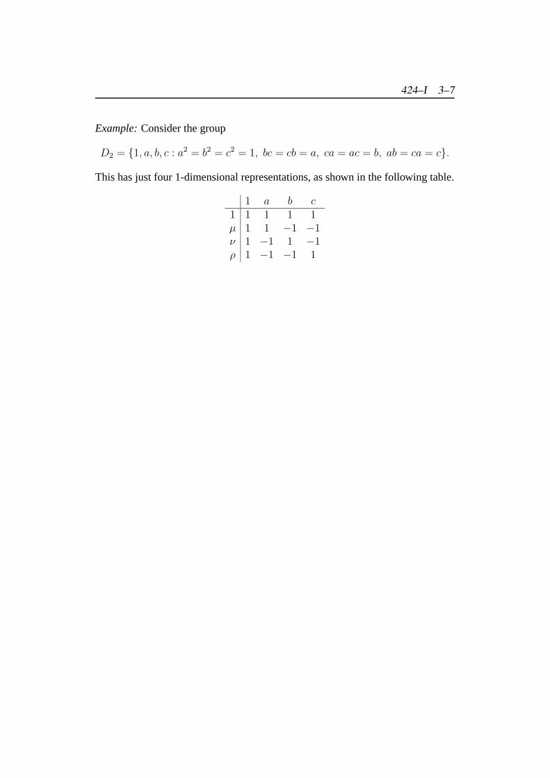
Example:Consider the group

D2 = {1, a, b, c : a2 = b2 = c2 = 1, bc = cb = a, ca = ac = b, ab = ca = c}.

This has just four 1-dimensional representations, as shown in the following table.

1 a b c1 1 1 1 1µ 1 1 −1 −1ν 1 −1 1 −1ρ 1 −1 −1 1

Chapter 4

The Arithmetic of Representations

4.1 Addition

Representations can be added and multiplied, like numbers; and the usuallaws of arithmetic hold. There is even a conjugacy operation, analogous tocomplex conjugation.

Definition 4.1 Supposeα, β are representations ofG in the vector spacesU, Voverk. Thenα + β is the representation ofG in U

⊕V defined by the action

g(u⊕ v) = gu⊕ gv.

Remarks:

1. Recall thatU⊕V is the cartesian product ofU andV , where however we

write u⊕ v rather than(u, v). The structure of a vector space is defined onthis set in the natural way.

2. Note thatα + β is only defined whenα, β are representations of thesamegroupG over thesamescalar fieldk.

3. Supposeα, β are given in matrix form

α : g 7→ A(g), β : g 7→ B(g).

Thenα + β is the representation

g 7→(A(g) 0

0 B(g)

)

424–I 4–1

4.2. MULTIPLICATION 424–I 4–2

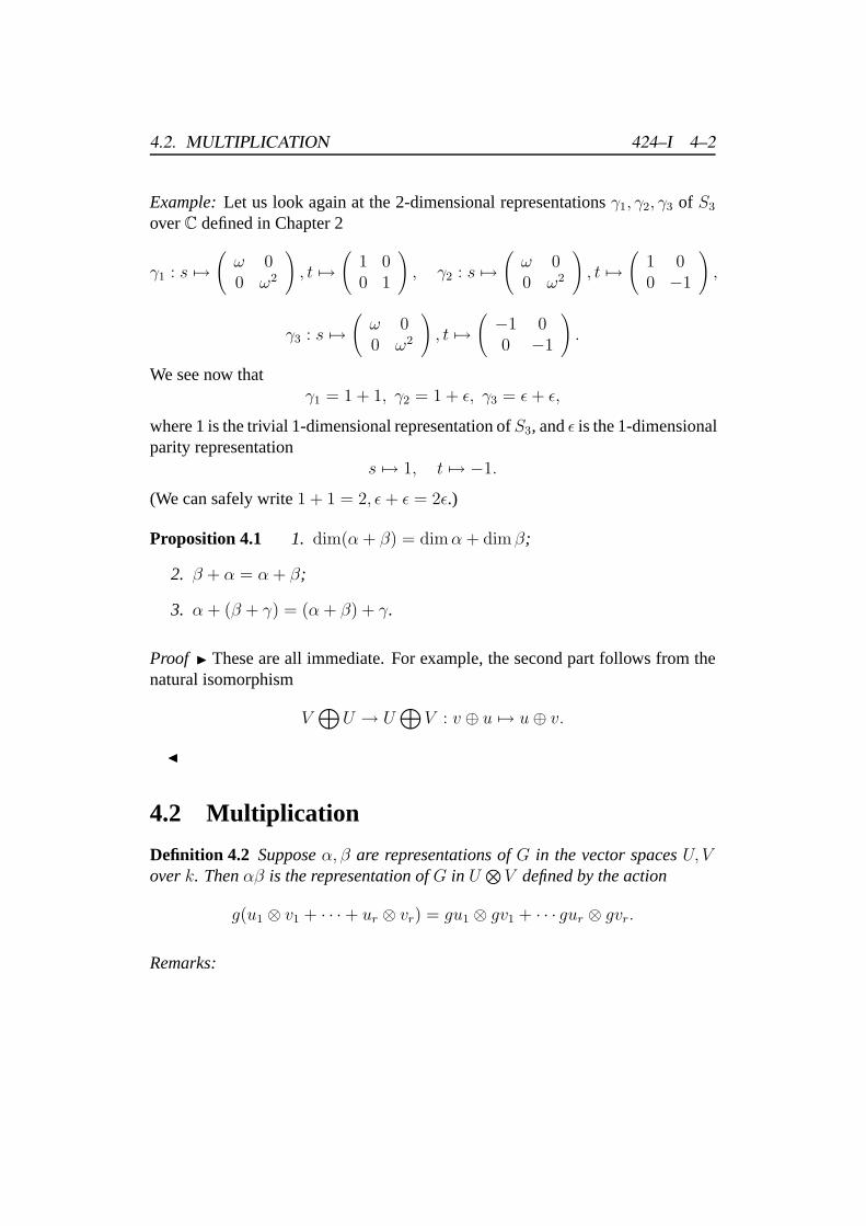
Example:Let us look again at the 2-dimensional representationsγ1, γ2, γ3 of S3

overC defined in Chapter 2

γ1 : s 7→(ω 00 ω2

), t 7→

(1 00 1

), γ2 : s 7→

(ω 00 ω2

), t 7→

(1 00 −1

),

γ3 : s 7→(ω 00 ω2

), t 7→

(−1 00 −1

).

We see now thatγ1 = 1 + 1, γ2 = 1 + ε, γ3 = ε+ ε,

where 1 is the trivial 1-dimensional representation ofS3, andε is the 1-dimensionalparity representation

s 7→ 1, t 7→ −1.

(We can safely write1 + 1 = 2, ε+ ε = 2ε.)

Proposition 4.1 1. dim(α + β) = dimα + dim β;

2. β + α = α + β;

3. α + (β + γ) = (α + β) + γ.

Proof I These are all immediate. For example, the second part follows from thenatural isomorphism

V⊕

U → U⊕

V : v ⊕ u 7→ u⊕ v.

J

4.2 Multiplication

Definition 4.2 Supposeα, β are representations ofG in the vector spacesU, Voverk. Thenαβ is the representation ofG in U

⊗V defined by the action

g(u1 ⊗ v1 + · · ·+ ur ⊗ vr) = gu1 ⊗ gv1 + · · · gur ⊗ gvr.

Remarks:

4.2. MULTIPLICATION 424–I 4–3

1. Thetensor productU⊗V of 2 vector spacesU andV may be unfamiliar.

Each element ofU⊗V is expressible as a finite sum

u1 ⊗ v1 + · · ·+ ur ⊗ vr.

If U has basis{e1, . . . , em} andV has basis{f1, . . . , fn} then themn ele-ments

ui ⊗ vj (i = 1, . . . ,m; j = 1, . . . , n)

form a basis forU⊗V . In particular

dim(U ⊗ V ) = dimU dimV.

(It is a common mistake to suppose that every element ofU⊗V is express-

ible in the formu ⊗ v. That is not so; the general element requires a finitesum.)

Formally, the tensor product is defined as the set of formal sums

u1 ⊗ v1 + · · ·+ ur ⊗ vr,

where 2 sums define the same element if one can be derived from the otherby applying the rules

(u1+u2)⊗v⊗u1⊗v+u2⊗v, u⊗(v1+v2)⊗u⊗v1+u⊗v2, (ρu)⊗v = u⊗(ρv).

The structure of a vector space is defined on this set in the natural way.

2. As withα+β, αβ is only defined whenα, β are representations of the samegroupG over the same scalar fieldk.

3. It is importantnot to write α × β for αβ, as we shall attach a differentmeaning toα× β later.

4. Supposeα, β are given in matrix form

α : g 7→ A(g), β : g 7→ B(g).

Thenαβ is the representation

αβ : g 7→ A(g)⊗B(g).

But what do we mean by the tensor productS ⊗ T of 2 square matricesS, T? If S = sij is anm×m-matrix, andT = tkl is ann× n-matrix, then

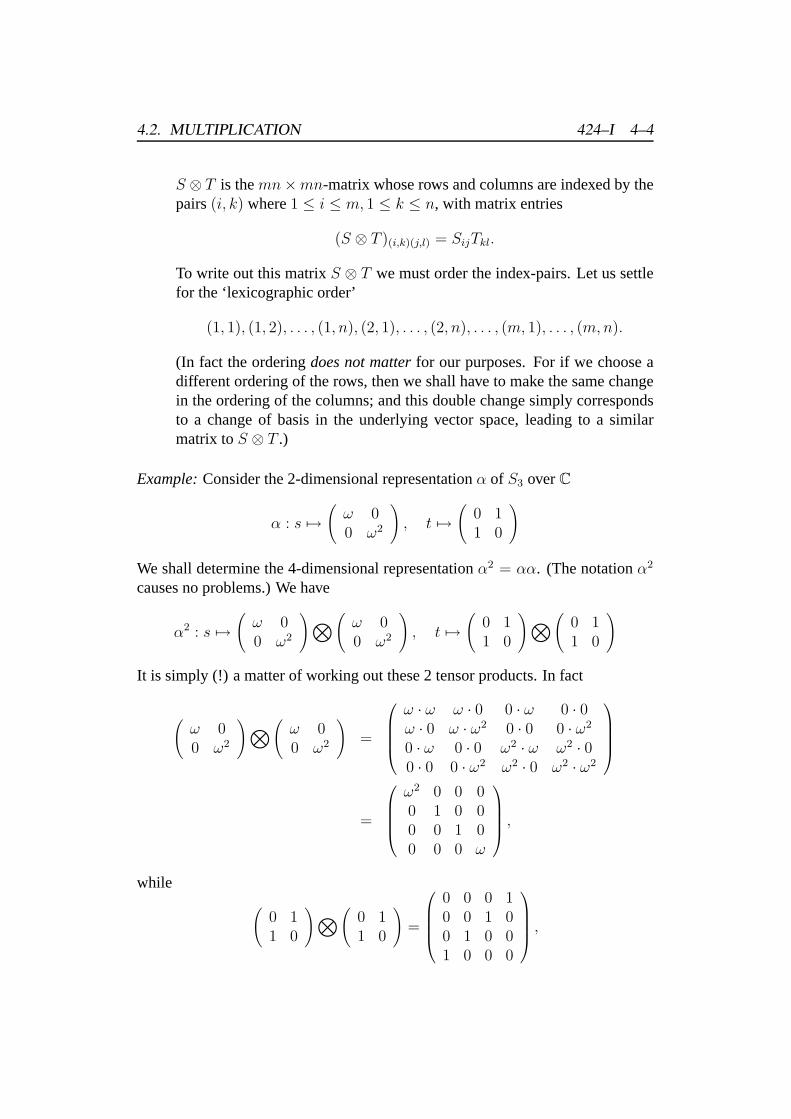
4.2. MULTIPLICATION 424–I 4–4

S ⊗ T is themn×mn-matrix whose rows and columns are indexed by thepairs(i, k) where1 ≤ i ≤ m, 1 ≤ k ≤ n, with matrix entries

(S ⊗ T )(i,k)(j,l) = SijTkl.

To write out this matrixS ⊗ T we must order the index-pairs. Let us settlefor the ‘lexicographic order’

(1, 1), (1, 2), . . . , (1, n), (2, 1), . . . , (2, n), . . . , (m, 1), . . . , (m,n).

(In fact the orderingdoes not matterfor our purposes. For if we choose adifferent ordering of the rows, then we shall have to make the same changein the ordering of the columns; and this double change simply correspondsto a change of basis in the underlying vector space, leading to a similarmatrix toS ⊗ T .)

Example:Consider the 2-dimensional representationα of S3 overC

α : s 7→(ω 00 ω2

), t 7→

(0 11 0

)

We shall determine the 4-dimensional representationα2 = αα. (The notationα2

causes no problems.) We have

α2 : s 7→(ω 00 ω2

)⊗(ω 00 ω2

), t 7→

(0 11 0

)⊗(0 11 0

)

It is simply (!) a matter of working out these 2 tensor products. In fact

(ω 00 ω2

)⊗(ω 00 ω2

)=

ω · ω ω · 0 0 · ω 0 · 0ω · 0 ω · ω2 0 · 0 0 · ω2

0 · ω 0 · 0 ω2 · ω ω2 · 00 · 0 0 · ω2 ω2 · 0 ω2 · ω2

=

ω2 0 0 00 1 0 00 0 1 00 0 0 ω

,

while (0 11 0

)⊗(0 11 0

)=

0 0 0 10 0 1 00 1 0 01 0 0 0

,

4.2. MULTIPLICATION 424–I 4–5

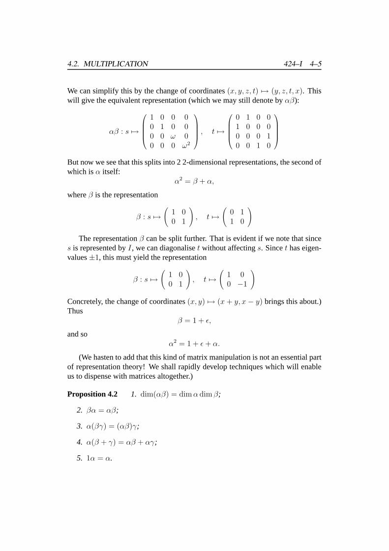
We can simplify this by the change of coordinates(x, y, z, t) 7→ (y, z, t, x). Thiswill give the equivalent representation (which we may still denote byαβ):

αβ : s 7→

1 0 0 00 1 0 00 0 ω 00 0 0 ω2

, t 7→

0 1 0 01 0 0 00 0 0 10 0 1 0

But now we see that this splits into 2 2-dimensional representations, the second ofwhich isα itself:

α2 = β + α,

whereβ is the representation

β : s 7→(

1 00 1

), t 7→

(0 11 0

)

The representationβ can be split further. That is evident if we note that sinces is represented byI, we can diagonaliset without affectings. Sincet has eigen-values±1, this must yield the representation

β : s 7→(

1 00 1

), t 7→

(1 00 −1

)

Concretely, the change of coordinates(x, y) 7→ (x+ y, x− y) brings this about.)Thus

β = 1 + ε,

and soα2 = 1 + ε+ α.

(We hasten to add that this kind of matrix manipulation is not an essential partof representation theory! We shall rapidly develop techniques which will enableus to dispense with matrices altogether.)

Proposition 4.2 1. dim(αβ) = dimα dim β;

2. βα = αβ;

3. α(βγ) = (αβ)γ;

4. α(β + γ) = αβ + αγ;

5. 1α = α.

4.3. CONJUGACY 424–I 4–6

All these results, again, are immediate consequences of ‘canonical isomor-phisms’ which it would be tedious to explicate.

We have seen that the representations ofG overk can be added and multiplied.They almost form a ring—only subtraction is missing. In fact if we introduce‘virtual representations’α−β (whereα, β are representations) then we will indeedobtain a ring

R(G) = R(G, k),

therepresentation-ringif G overk. (By convention ifk is omitted then we assumethatk = C.)

We shall see later that

α + β = α + γ =⇒ β = γ.

It follows that nothing is lost in passing from representations toR(G); if α = βin R(G) thenα = β in ‘real life’.

4.3 Conjugacy

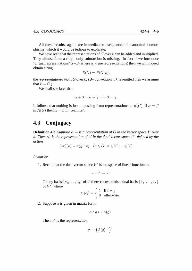
Definition 4.3 Supposeα = is a representation ofG in the vector spaceV overk. Thenα∗ is the representation ofG in the dual vector spaceU∗ defined by theaction

(gπ)(v) = π(g−1v) (g ∈ G, π ∈ V ∗, v ∈ V )

Remarks:

1. Recall that the dual vector spaceV ∗ is the space of linear functionals

π : V → k.

To any basis{e1, . . . , en} of V there corresponds a dual basis{π1, . . . , πn}of V ∗, where

πj(ei) =

{1 if i = j0 otherwise

2. Supposeα is given in matrix form

α : g 7→ A(g).

Thenα∗ is the representation

g 7→(A(g)−1

)′,

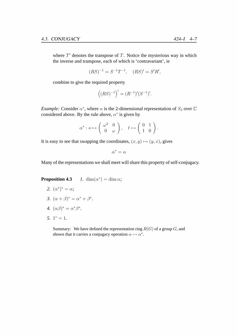
4.3. CONJUGACY 424–I 4–7

whereT ′ denotes the transpose ofT . Notice the mysterious way in whichthe inverse and transpose, each of which is ‘contravariant’, ie

(RS)−1 = S−1T−1, (RS)′ = S ′R′,

combine to give the required property((RS)−1

)′= (R−1)′(S−1)′.

Example:Considerα∗, whereα is the 2-dimensional representation ofS3 overCconsidered above. By the rule above,α∗ is given by

α∗ : s 7→(ω2 00 ω

), t 7→

(0 11 0

).

It is easy to see that swapping the coordinates,(x, y) 7→ (y, x), gives

α∗ = α

Many of the representations we shall meet will share this property of self-conjugacy.

Proposition 4.3 1. dim(α∗) = dimα;

2. (α∗)∗ = α;

3. (α + β)∗ = α∗ + β∗.

4. (αβ)∗ = α∗β∗.

5. 1∗ = 1.

Summary: We have defined the representation ringR(G) of a groupG, andshown that it carries a conjugacy operationα 7→ α∗.

Chapter 5

Semisimple Representations

Definition 5.1 The represenationα ofG is said to besemisimpleif it is express-ible as a sum of simple representations:

α = σ1 + · · ·+ σr.

Example:Consider the permutation representationρ of S3 in k3. (It doesn’t matterfor the following argument ifk = R orC.)

Recall thatg(x1, x2, x3) = (xg−11, xg−12, xg−13).

We have seen thatk3 has 2 proper stable subspaces:

U = {(x, x, x) : x ∈ k}, W = {(x1, x2, x3) : x1 + x2 + x3 = 0}.

U has dimension 1, with basis{(1, 1, 1)};W has dimension 2, with basis{(1,−1, 0), (−1, 0, 1)}.Evidently

U ∩ V = 0.

Recall that a sumU + V of vector subspaces is direct,

U + V = U ⊕ V,

if (and only if)U ∩ V = 0. So it follows here, by considering dimensions, that

k3 = U⊕

W.

The representation onU is the trivial representation 1. Thus

ρ = 1 + α,

whereα is the representation ofS3 in W .

424–I 5–1

424–I 5–2

We can see thatα is simple as follows. SupposeV ⊂ W is stable underS3,whereV 6= 0. Take any elementv 6= 0 in V : say

v = (x, y, z) (x+ y + z = 0).

The coefficientsx, y, z cannot all be equal. Supposex 6= y. Then

(12)v = (y, x, z) ∈ V ;

and sov − (12)v = (x− y, y − x, 0) = (x− y)(1,−1, 0) ∈ V.

Hence(1,−1, 0) ∈ V.

It follows that(−1, 0, 1) = (132)(1,−1, 0) ∈ V

also. But these 2 elements generate W; hence

V = W.

So we have shown thatW is a simpleS3-space, whence the corresponding repre-sentationα is simple.

We conclude that the representation

ρ = 1 + α

is a sum of simple representations, and so is semisimple.It is easy to see thatU andW are the only subspaces ofk3 stable underS3,

apart from 0 and the whole space. So it is evident that the splittingU ⊕ V isunique. In general this is not so; in fact we shall show later that there is a uniquesplit into simple subspaces if and only if the representations corresponding tothese subspaces are distinct. (So in this case the split is unique because1 6= α.)However the simple representations that appearare unique. This fact, which weshall prove in the next chapter, is the foundation stone of representation theory.

Most of the time we do not need to look behind a representation at the un-derlying representation-space. But sometimes we do; and the following resultsshould help to clarify the structure of semisimple representation-spaces.

Proposition 5.1 SupposeV is a sum (not necessarily direct) of simple subspaces:

V = S1 + · · ·+ Sr.

ThenV is semisimple.

424–I 5–3

Proof I SinceS2 is simple,

S1 ∩ S2 = 0 or S2.

In the former caseS1 + S2 = S1

⊕S2;

in the latter caseS2 ⊂ S1 and so

S1 + S2 = S1.

Repeating the argument withS1 + S2 in place ofS1, andS3 in place ofS2,

(S1 + S2) ∩ S3 = 0 or S3,

sinceS3 is simple. In the former case

S1 + S2 + S3 = (S1 + S2)⊕

S3;

in the latter caseS3 ⊂ S1 + S2 and so

S1 + S2 + S3 = S1 + S2.

Combining this with the previous step

S1 + S2 + S3 = S1

⊕S2

⊕S3 or S1

⊕S3 or S1

⊕S2 or S1.

Continuing in this style, at theith step, sinceSi is simple,

S1 + · · ·+ Si = (S1 + · · ·+ Si−1)⊕

Si or S1 + · · ·+ Si−1.

We conclude, finally, that

V = S1 + · · ·+ Sr = Si1⊕· · ·Sis ,

where{Si1 , . . . , Sis} is a subset of{S1, . . . , Sr}. J

Remark:The subset{Si1 , . . . , Sis} depends in general on theorder in which wetakeS1, . . . , Sr. In particular, sinceSi1 = S1, we can always specify that anyoneof S1, . . . , Sn appears in the direct sum.

Proposition 5.2 The following 2 properties of theG-spaceV are equivalent:

1. V is semisimple;

424–I 5–4

2. each stable subspaceU ⊂ V has at least one complementary stable sub-spaceW , ie

V = U⊕

W.

Proof I Suppose first thatV is semisimple, say

V = S1

⊕· · ·

⊕Sr.

Let us follow the proof of the preceding proposition, but starting withU ratherthanS1. Thus our first step is to note that sinceS1 is simple,

U + S1 = U⊕

S1 orU.

Continuing as before, we conclude that

V = U⊕

Si1⊕· · ·

⊕Sis ,

from which the result follows, with

W = Si1⊕· · ·

⊕Sis .

Now suppose that condition (2) holds. SinceV is finite-dimensional, we canfind a stable subspaceS1 of minimal dimension. EvidentlyS1 is simple; and byour hypothesis

V = S1

⊕W1.

Now let us find a stable subspaceS2 of W1 of minimal dimension. As before,this subspace is simple; and

S1 ∩ S2 ⊂ S1 ∩W = 0,

so thatS1 + S2 = S1

⊕S2.

Applying the hypothesis again to this space, we can find a stable complementW2:

V = S1

⊕S2

⊕W2.

Continuing in this way, sinceV is finite-dimensional we must conclude withan expression forV as a direct sum of simple subspaces:

V = S1

⊕· · ·

⊕Sr.

HenceV is semisimple. J

Remark: This Proposition gives an alternative definition of semisimplicity:Vis semisimple if every stable subspaceU ⊂ V posseses a complementary sta-ble subspaceW . This alternative definition allows us to extend the concept ofsemisimplicity to infinite-dimensional representations.

424–I 5–5

Exercises

In Exercises 01–15 calculateeX for the given matrixX:

1. Show that anycommutingset of diagonalisable matrices can be simultane-ously diagonalised. Hence show that any representation of a finite abeliangroup

2. Show that for alln the natural representationρ of Sn in kn is semisimple.

3. If T ∈ GL(n, k) then the map

Z→ GL(n, k) : m 7→ Tm

defines a representationτ of the infinite abelian groupZ.

Show that ifk = C thenτ is semisimple if and only ifT is semisimple.

4. Prove the same result whenk = R.

5. Supposek = GF(2) = {0, 1}, the finite field with 2 elements. Show thatthe representation ofC2 = {e, g} given by

g 7→(

1 10 1

)

is not semisimple.

Chapter 6

Every Representation of a FiniteGroup is Semisimple

Theorem 6.1 (Maschke’s Theorem) Supposeα is a representation of the finitegroupG overk, wherek = R or C. Thenα is semisimple.

Proof I Supposeα is a representation onV . We take the alternative definition ofsemisimplicity: every stable subspaceU ⊂ V must have a stable complementW .

Our idea is to construct an invariant positive-definite formP onV . (By ‘form’we mean herequadratic formif k = R, or hermitian formif k = C.) Then we cantakeW to be theorthogonal complementof U with respect to this form:

W = U⊥ = {v ∈ V : P (u, v) = 0 for all u ∈ U}.

We can construct such a form by takingany positive-definite formQ, andaveragingit over the group:

P (u, v) =1

‖G‖∑g∈G

Q(gu, gv).

(It’s not really necessary to divide by the order of the group; we do it because theidea of ‘averaging over the group’ occurs in other contexts.)

It is easy to see that the resulting form is invariant:

P (gu, gv) =1

‖G‖∑h∈G

Q(hgu, hgv)

=1

‖G‖∑h∈G

Q(hu, hv)

= P (u, v)

424–I 6–1

424–I 6–2

sincehg runs over the group ash does so.It is a straightforward matter to verify that ifP is invariant andU is stable then

so isU⊥. Writing 〈u, v〉 for P (u, v),

g ∈ G,w ∈ U⊥ =⇒ 〈u,w〉 = 0 ∀u ∈ U=⇒ 〈gu, gw〉 = 〈u,w〉 = 0 ∀u ∈ U=⇒ 〈u, gw〉 = 〈g(g−1u), w〉 = 0 ∀u ∈ U=⇒ gw ∈ U⊥.

J

Examples:

1. Consider the representation ofS3 in R3. There is an obvious invariantquadratic form—as is often the case—namely

x21 + x2

2 + x23.

But as an exercise in averaging, let us take the positive-definite form

Q(x1, x2, x3) = 2x21 − 2x1x2 + 3x2

2 + x23.

Then

Q (e(x1, x2, x3)) = Q(x1, x2, x3) = 2x21 − 2x1x2 + 3x2

2 + x23

Q ((23)(x1, x2, x3)) = Q(x1, x3, x2) = 2x21 − 2x1x3 + 3x2

3 + x22

Q ((13)(x1, x2, x3)) = Q(x3, x2, x1) = 2x23 − 2x3x2 + 3x2

2 + x21

Q ((12)(x1, x2, x3)) = Q(x2, x1, x3) = 2x22 − 2x2x1 + 3x2

1 + x23

Q ((123)(x1, x2, x3)) = Q(x3, x1, x2) = 2x23 − 2x3x1 + 3x2

1 + x22

Q ((132)(x1, x2, x3)) = Q(x2, x3, x1) = 2x22 − 2x2x3 + 3x2

3 + x21

Adding, and dividing by 6,

P (x1, x2, x3) = 2(x2

1 + x22 + x2

3

)− 2

3(x2x3 + x1x3 + x1x2)

=7

3

(x2

1 + x22 + x2

3

)− 1

3(x1 + x2 + x3)2 .

The corresponding inner product is given by

〈(x1, x2, x3), (y1, y2, y3)〉 = 2(x1y1+x2y2+x3y3)−1

3(x2y3+x3y2+x3y1+x1y3+x1y2+x2y1)

424–I 6–3

To see how this is used, let

U = {(x, x, x) : x ∈ R}.

EvidentlyU is stable. Its orthogonal complement with respect to the formabove is

U⊥ = {(x1, x2, x3) : 〈(1, 1, 1), (x1, x2, x3)〉 = 0}

= {(x1, x2, x3) :4

3(x1 + x2 + x3) = 0}

= {(x1, x2, x3) : x1 + x2 + x3 = 0},

which is just the complement we found before. This is not surprising since—as we observed earlier—U andU⊥ are the only proper stable subspaces ofR

3.

2. For an example using hermitian forms, consider the simple representationof D4 overC defined by

s 7→(i 00 −i

), t 7→

(0 11 0

).

Again, there is an obvious invariant hermitian form, namely

|x21 + x2

2| = x1x1 + x2x2.

But this will not give us much exercise.

The general hermitian form onC2 is

axx+ byy + cxy + cyx (a, b ∈ R, c ∈ C)

Let us takeQ(x, y) = 2xx+ yy − ixy + iyx.

Note thatD4 = {e, s, s2, s3, t, ts, ts2, ts3}.

For these 8 elements are certainly distinct, eg

s2 = ts3 =⇒ ts = 1 =⇒ s = t.

424–I 6–4

Now

Q (e(x, y)) = Q(x, y) = 2xx+ yy − ixy + iyx,

Q (s(x, y)) = Q(ix,−iy) = 2xx+ yy + ixy − iyx,Q(s2(x, y)

)= Q(−x,−y) = 2xx+ yy − ixy + iyx,

Q(s3(x, y)

)= Q(−ix, iy) = 2xx+ yy + ixy − iyx,

Q (t(x, y)) = Q(y, x) = xx+ 2yy + ixy − iyx,Q (ts(x, y)) = Q(iy,−ix) = xx+ 2yy − ixy + iyx,

Q(ts2(x, y)

)= Q(−y,−x) = xx+ 2yy + ixy − iyx,

Q(ts3(x, y)

)= Q(−iy, ix) = xx+ 2yy − ixy + iyx.

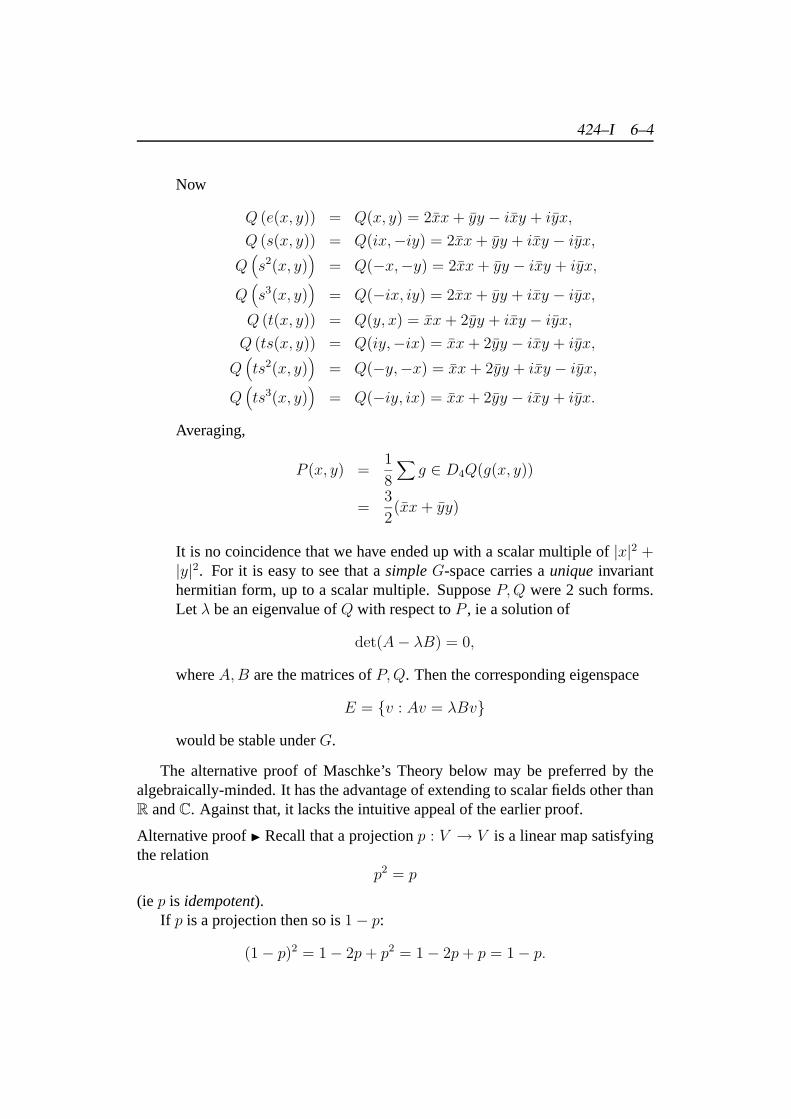
Averaging,

P (x, y) =1

8

∑g ∈ D4Q(g(x, y))

=3

2(xx+ yy)

It is no coincidence that we have ended up with a scalar multiple of|x|2 +|y|2. For it is easy to see that asimpleG-space carries auniqueinvarianthermitian form, up to a scalar multiple. SupposeP,Q were 2 such forms.Let λ be an eigenvalue ofQ with respect toP , ie a solution of

det(A− λB) = 0,

whereA,B are the matrices ofP,Q. Then the corresponding eigenspace

E = {v : Av = λBv}

would be stable underG.

The alternative proof of Maschke’s Theory below may be preferred by thealgebraically-minded. It has the advantage of extending to scalar fields other thanR andC. Against that, it lacks the intuitive appeal of the earlier proof.

Alternative proofI Recall that a projectionp : V → V is a linear map satisfyingthe relation

p2 = p

(ie p is idempotent).If p is a projection then so is1− p:

(1− p)2 = 1− 2p+ p2 = 1− 2p+ p = 1− p.

424–I 6–5

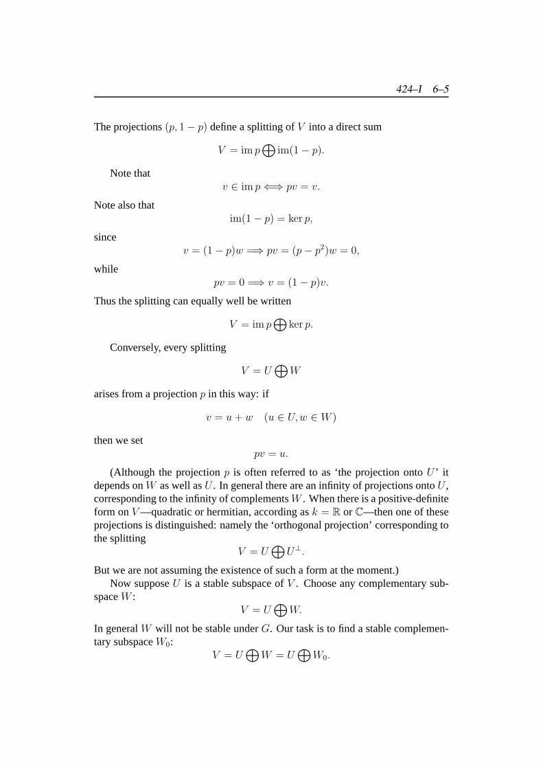
The projections(p, 1− p) define a splitting ofV into a direct sum

V = im p⊕

im(1− p).

Note thatv ∈ im p⇐⇒ pv = v.

Note also thatim(1− p) = ker p,

sincev = (1− p)w =⇒ pv = (p− p2)w = 0,

whilepv = 0 =⇒ v = (1− p)v.

Thus the splitting can equally well be written

V = im p⊕

ker p.

Conversely, every splitting

V = U⊕

W

arises from a projectionp in this way: if

v = u+ w (u ∈ U,w ∈ W )

then we setpv = u.

(Although the projectionp is often referred to as ‘the projection ontoU ’ itdepends onW as well asU . In general there are an infinity of projections ontoU ,corresponding to the infinity of complementsW . When there is a positive-definiteform onV—quadratic or hermitian, according ask = R orC—then one of theseprojections is distinguished: namely the ‘orthogonal projection’ corresponding tothe splitting

V = U⊕

U⊥.

But we are not assuming the existence of such a form at the moment.)Now supposeU is a stable subspace ofV . Choose any complementary sub-

spaceW :V = U

⊕W.

In generalW will not be stable underG. Our task is to find a stable complemen-tary subspaceW0:

V = U⊕

W = U⊕

W0.

424–I 6–6

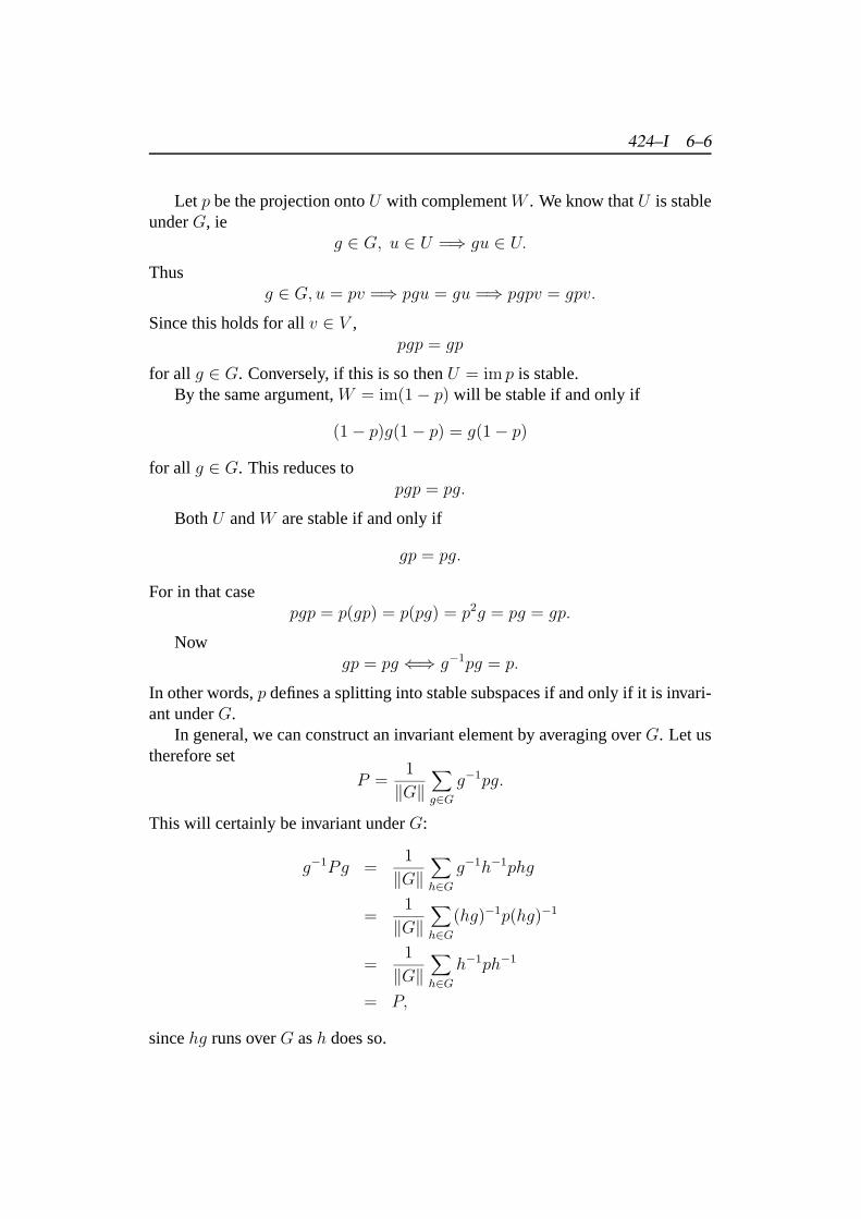
Let p be the projection ontoU with complementW . We know thatU is stableunderG, ie

g ∈ G, u ∈ U =⇒ gu ∈ U.

Thusg ∈ G, u = pv =⇒ pgu = gu =⇒ pgpv = gpv.

Since this holds for allv ∈ V ,pgp = gp

for all g ∈ G. Conversely, if this is so thenU = im p is stable.By the same argument,W = im(1− p) will be stable if and only if

(1− p)g(1− p) = g(1− p)

for all g ∈ G. This reduces topgp = pg.

BothU andW are stable if and only if

gp = pg.

For in that casepgp = p(gp) = p(pg) = p2g = pg = gp.

Nowgp = pg ⇐⇒ g−1pg = p.

In other words,p defines a splitting into stable subspaces if and only if it is invari-ant underG.

In general, we can construct an invariant element by averaging overG. Let ustherefore set

P =1

‖G‖∑g∈G

g−1pg.

This will certainly be invariant underG:

g−1Pg =1

‖G‖∑h∈G

g−1h−1phg

=1

‖G‖∑h∈G

(hg)−1p(hg)−1

=1

‖G‖∑h∈G

h−1ph−1

= P,

sincehg runs overG ash does so.

424–I 6–7

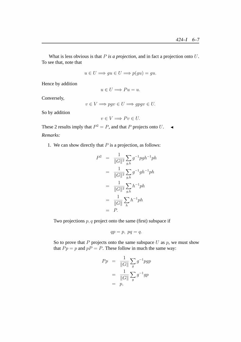
What is less obvious is thatP is a projection, and in fact a projection ontoU .To see that, note that

u ∈ U =⇒ gu ∈ U =⇒ p(gu) = gu.

Hence by additionu ∈ U =⇒ Pu = u.

Conversely,v ∈ V =⇒ pgv ∈ U =⇒ gpgv ∈ U.

So by additionv ∈ V =⇒ Pv ∈ U.

These 2 results imply thatP 2 = P , and thatP projects ontoU . J

Remarks:

1. We can show directly thatP is a projection, as follows:

P 2 =1

‖G‖2

∑g,h

g−1pgh−1ph

=1

‖G‖2

∑g,h

g−1gh−1ph

=1

‖G‖2

∑g,h

h−1ph

=1

‖G‖∑h

h−1ph

= P.

Two projectionsp, q project onto the same (first) subspace if

qp = p, pq = q.

So to prove thatP projects onto the same subspaceU asp, we must showthatPp = p andpP = P . These follow in much the same way:

Pp =1

‖G‖∑g

g−1pgp

=1

‖G‖∑g

g−1gp

= p,

424–I 6–8

pP =1

‖G‖∑g

pg−1pg

=1

‖G‖∑g

g−1pg

= P.

2. Both proofs of Maschke’s Theorem rely on the same idea: obtaining aninvariant element (in the first proof, an invariant form; in the second, andinvariant projection) by averaging over transforms of a non-invariant ele-ment.

In general, ifV is aG-space (in other words, we have a representation ofGin V ) then the invariant elements form a subspace

V G = {v ∈ V : gv = v∀g ∈ G}.

The averaging operation defines a projection ofV ontoV G:

v 7→ 1

‖G‖∑g

gv.

ClearlyV G is a stable subspace ofV . Thus ifV is simple, eitherV G = 0or V G = V . In the first case, all averages vanish. In the second case, therepresentation inV is trivial, and soV must be 1-dimensional.

3. It is worth noting that our alternative proof works in any scalar fieldk,provided‖G‖ 6= 0 in k. Thus it even works over the finite fieldGF(pn),unlessp | ‖G‖.Of course we are not considering suchmodular representations(as rep-resentations over finite fields are known); but our argument shows thatsemisimplicity still holds unless the characteristicp if the scalar field di-vides the order of the group.

Chapter 7

Uniqueness and the IntertwiningNumber

Definition 7.1 Supposeα, β are representations ofG overk in the vector spacesU, V respectively. Theintertwining numberI(α, β) is defined to be the dimensionof the space ofG-mapst : U → V ,

I(α, β) = dim homG(U, V ).

Remarks:

1. AG-mapt : U → V is a linear map which preserves the action ofG:

t(gu) = g(tu) (g ∈ G, u ∈ G).

TheseG-maps evidently form a vector space overk.

2. The intertwining number will remain somewhat abstract until we give aformula for it (in terms of characters) in Chapter . But intuitivelyI(α, β)measures how much the representationsα, β have in common.

3. The intertwining number of finite-dimensional representations is certainlyfinite, as the following result shows.

Proposition 7.1 We have

I(α, β) ≤ dimα dim β.

Proof I The spacehom(U, V ) of all linear mapst : U → V has dimensiondimU dimV , since we can represent each such map by anm × n-matrix, wherem = dimU, n = dimV .

424–I 7–1

424–I 7–2

The result follows, since

homG(U, V ) ⊂ hom(U, V ).

J

Proposition 7.2 Supposeα, β aresimplerepresentations overk. Then

I(α, β) =

{0 if α 6= β,≥ 1 if α = β.

Proof I Supposeα, β are representations inU, V , respectively; and suppose

t : U → V

is aG-map. Then the subspaces

ker t = {u ∈ U : tu = 0} and im t = {v ∈ V : ∃u ∈ U, tu = v}

are both stable underG. Thus

u ∈ ker t =⇒ tu = 0

=⇒ t(gu) = g(tu) = 0

=⇒ gu ∈ ker t,

while

v ∈ im t =⇒ v = tu

=⇒ t(gu) = g(tu) = gv

=⇒ gv ∈ im t.

But sinceU andV are both simple, by hypothesis, it follows that

ker t = 0 orU, im t = 0 or V.

Now ker t = U =⇒ t = 0, andim t = 0 =⇒ t = 0. So if t 6= 0,

ker t = 0, im t = V.

But in this caset is anisomorphismof G-spaces, and soα = β.On the other hand, ifα = β then (by the definition of equivalent representa-

tions) there exists aG-isomorphist : U → V , and soI(α, β) ≥ 1. J

Whenk = C we can be more precise.

424–I 7–3

Proposition 7.3 If α is a simple representation overC then

I(α, α) = 1.

Proof I SupposeV carries the representationα. We have to show that

dim homG(V, V ) = 1.

Since the identity map1 : V → V is certainly aG-map, we have to show thateveryG-mapt : V → V is a scalar multipleρ1 of the identity.

Let λ be an eigenvector oft. Then the corresponding eigenspace

E = E(λ) = {v ∈ V : tv = λv}

is stable underG. For

g ∈ G, v ∈ E =⇒ t(gv) = g(tv) = λgv =⇒ gv ∈ E.

Sinceα is simple, this implies thatE = V , ie

t = λ1.

J

Proposition 7.4 Supposeα, β, γ are representations overk. Then

1. I(α + β, γ) = I(α, γ) + I(β, γ);

2. I(α, β + γ) = I(α, β) + I(α, γ);

3. I(αβ, γ) = I(α, β∗γ).

Proof I Supposeα, β, γ are representations inU, V,W respectively. The first 2results are immediate, arising from the more-or-less self-evident isomorphisms

hom(U⊕

V,W ) ∼= hom(U,W )⊕

hom(V,W )

hom(U, V⊕

W ) ∼= hom(U, V )⊕

hom(U,W ).

Take the first. This expresses the fact that a linear map

t : U⊕

V → W

can be defined by giving 2 linear maps

t1 : U → W, t2 : V → W.

424–I 7–4

In fact t1 is the restriction oft to U ⊂ U⊕V , and t2 the restriction oft to

V ⊂ U⊕V ; and

t(u⊕ v) = t1u⊕ t2v.

In much the same way, the second result expresses the fact that a linear map

t : U → V⊕

W

can be defined by giving 2 linear maps

t1 : U → V, t2 : U → W.

In factt1 = π1t, t2 = π2t,

whereπ1, π2 are the projections ofU⊕V ontoV,W respectively; and

tu = t1u⊕ t2u.

The third result, although following from a similar ‘natural equivalence’

hom(U⊗

V,W ) ∼= hom(U, V ∗⊗

W ),

whereV ∗ = hom(V, k),

is rather more difficult to establish.We can divide the task in two. First, there is a natural equivalence

hom(U,hom(V,W )) ∼= hom(U⊗

V,W ).

For this, note that there is a 1–1 correspondence betweenlinearmapsb : U⊗V →

W andbilinear mapsB : U × V → W.

(This is sometimes taken as the definition ofU⊗V .) So we have to show how

such a bilinear mapB(u, v) gives rise to a linear map

t : U → hom(V,W ).

But that is evident:t(u)(v) = B(u, v).

It is a straightforward matter to verify that every such linear mapt arises in thisway from a unique bilinear mapB.

424–I 7–5

It remains to show that

hom(V,W ) ∼= V ∗⊗

W.

For this, note first that both sides are ‘additive functors’ inW , ie

hom(V,W1

⊕W2) = hom(V,W1)

⊕hom(V,W2),

V ∗⊗

(W1

⊕W2) = (V ∗

⊗W1)

⊕(V ∗

⊗W2).

This allows us to reduce the problem, by expressingW as a sum of 1-dimensionalsubspaces, to the case whereW is 1-dimensional. In that case, we may takeW = k; so the result to be proved is

hom(V, k) ∼= V ∗⊗

k.

But there is a natural isomorphism

U⊗

k ∼= U

for every vector spaceU . So our result reduces to the tautologyV ∗ ∼= V ∗.It’s a straightforward (if tedious) matter to verify that these isomorphisms are

all compatible with the actions of the groupG. In particular theG-invariant ele-ments on each side correspond:

homG(U⊕

V,W ) ∼= homG(U,W )⊕

homG(V,W ),

homG(U, V⊕

W ) ∼= homG(U, V )⊕

homG(U,W ),

homG(U⊗

V,W ) ∼= homG(U, V ∗⊗

W ).

The 3 results follow on taking the dimensions of each side.J

Theorem 7.1 The expression for a semisimple representationα as a sum of sim-ple parts

α = σ1 + · · ·+ σr

is unique up to order.

Proof I Supposeσ is a simple representation ofG overk. We can use the inter-twining number to compute the number of times,m say, thatσ occurs amongsttheσi. For

I(σ, α) = I(σ, σ1) + · · ·+ I(σ, σr)

= mI(σ, σ),

424–I 7–6

since only those summands for whichσi = σ will contribute to the sum. Thus

m =I(σ, α)

I(σ, σ).

It follows thatσ will occur the same numberm times in every expression forαas a sum of simple parts. Hence two such expressions can only differ in the orderof their summands. J

Although the expression

α = σ1 + · · ·+ σr

for the representationα is unique, the corresponding splitting

V = U1

⊕· · ·

⊕Ur

of the representation-space is not in general unique. It’s perfectly possible for 2different expressions forV as a direct sum of simpleG-subspaces to give rise tothesameexpression forα: say

V = U1

⊕· · ·

⊕Ur, V = W1

⊕· · ·

⊕Wr

whereUi andWi both carry the representationσi.For example, consider the trivial representationα = 1 + 1 of a groupG in the

2-dimensional spaceV = k2. Every subspace ofV is stable underG; so if wechooseany2 different 1-dimensional subspacesU,W ⊂ V , we will have

V = U⊕

W.

However, the splitting ofV into isotypic componentsis unique, as we shallsee.

Definition 7.2 The representationα, and the underlying representation-spaceV ,are said to beisotypicof typeσ, whereσ is a simple representation, if

α = eσ = σ + · · ·+ σ.

In other words,σ is the only simple representation appearing inα.

Proposition 7.5 SupposeV is aG-space.

1. If V is isotypic of typeσ then so is everyG-subspaceU ⊂ V .

2. If U,W ⊂ V are isotypic of typeσ then so isU +W .

424–I 7–7

Proof I These results follow easily from the Uniqueness Theorem. But it is usefulto give an independent proof, since we can use this to construct an alternativeproof of the Uniqueness Theorem.

Lemma 7.1 SupposeV = U1 + · · ·+ Ur

is an expression for theG-spaceV as a sum of simple spaces; and suppose thesubspaceU ⊂ V is also simple. ThenU is isomorphic (as aG-space) to one ofthe summands:

U ∼= Ui

for somei.

Proof of LemmaBWe know that

V = Ui1⊕· · ·

⊕Uit

for some subset{Ui1 , . . . , Uit} ⊂ {U1, . . . , Ur}. Thus we may assume that thesum is direct:

V = U1

⊕· · ·

⊕Ur.

For eachi, consider the composition

U → V → Ui,

where the second map is the projection ofV onto its componentUi. SinceU andUi are both simple, this map is either an isomorphism, or else 0.

But it cannot be 0 for alli. For supposeu ∈ U, u 6= 0. We can expressu as asum

u = u1 ⊕ · · · ⊕ ur (ui ∈ Ui).Not all theui vanish. Nowu 7→ ui under the compositionU → V → Ui. Thusone (at least) of these compositions is6= 0. HenceU ∼= Ui for somei. C

Turning to the first part of the Proposition, ifU ⊂ V , whereV is σ-isotypic,then each simple summand ofU must be of typeσ, by the Lemma. It follows thatU is alsoσ-isotypic.

For the second part, ifU andW are bothσ-isotypic, thenU +W is a sum (notnecessarily direct) of simple subspacesXi of typeσ:

U +W = X1 + · · ·+Xr.

But thenU +W = Xi1

⊕· · ·

⊕Xit ,

where{Xi1 , . . . , Xit} are some of theX1, . . . , Xr. In particularU + W is σ-isotypic. J

424–I 7–8

Corollary 7.1 Supposeσ is a simple representation ofG overk, Then eachG-spaceV overk possesses a maximalσ-isotypic subspaceVσ, which contains everyotherσ-isotypic subspace.

Definition 7.3 This subspaceVσ is called theσ-component ofV .

Proposition 7.6 Every semimsimpleG-spaceV is the direct sum of its isotypiccomponents:

V = Vσ1

⊕· · ·

⊕Vσr .

Proof I If we take an expression forV as a direct sum of simple subspaces, andcombine those that are isomorphic, we will obtain an expression forV as a directsum of isotypic spaces of different types, each of which will be contained in thecorresponding isotypic component. It follows that

V = Vσ1 + · · ·+ Vσr .

We have to show that this sum is direct.It is sufficient to show that

(Vσ1 + · · ·+ Vσi−1)⋂Vσi = 0

for i = 2, . . . , r.Suppose not. Then we can find a simple subspace

U ⊂ Vσi , U ⊂ Vσ1 + · · ·+ Vσi−1.

By the Lemma to the last Proposition,U must be of typeσi, as a subspace ofVσi.On the other hand, as a subspace ofVσ1 + · · ·+Vσi−1

it must be of one of the typesσ1, . . . , σi−1, by the same Lemma.

This is a contradiction. Hence the sum is direct:

V = Vσ1

⊕· · ·

⊕Vσr .

J

Corollary 7.2 If theG-spaceV carries a multiple-free representation

α = σ1 + · · ·+ σr

(where theσi are distinct) thenV has a unique expression as a direct sum ofsimple subspaces.

424–I 7–9

Remark:It is easy to see that multiplicitydoesgive rise to non-uniqueness. Forsuppose

V = U⊕

U,

whereU is simple. For eachλ ∈ k consider the map

u 7→ u⊕ λu : U → U⊕

U = V.

The image of this map is a subspace

U(λ) = {u⊕ λu : u ∈ U}.

This subspace is isomorphic toU , sinceU is simple.It is readily verified that

U(λ) 6= U(µ)⇐⇒ λ = µ.

It follows thatV = U(λ)

⊕U(µ)

for anyλ, µ with λ 6= µ.

Chapter 8

The Character of a Representation

Amazingly, all the information about a representation of a groupG can beencoded in a single function onG, thecharacterof the representation.

Definition 8.1 Supposeα is a representation ofG overk. Thecharacterχ = χαof α is the functionχ : G→ k defined by

χ(g) = tr (α(g)) .

Remarks:

1. Recall that thetraceof ann × n-matrixA is the sum of the diagonal ele-ments:

trA =∑

1≤i≤nAii.

The trace has the following properties:

(a) tr(A+B) = trA+ trB;

(b) tr(λA) = λ trA.

(c) trAB = trBA;

(d) trA′ = trA;

(e) trA∗ = trA.

HereA′ denotes the transpose ofA, andA∗ the conjugate transpose:

A′ij = Aji, A∗ij = Aji.

The third property is the only one that is not immediate:

trAB =∑i

(AB)ii =∑i

∑j

AijBji =∑j

∑i

BjiAij = trBA.

424–I 8–1

424–I 8–2

Note thattrABC 6= trBAC

in general. However the traceis invariant undercyclicpermutations, eg

trABC = trBCA = trCAB.

In particular, ifP is invertible (non-singular) then

trPAP−1 = trP−1PA = trA :

similar matrices have the same trace.

It follows from this that we can speak without ambiguity of the tracetr tof a linear transformationt : V → V ; for the matrixT representingt withrespect to one basis will be changed toPTP−1 with respect to another basis,whereP is the matrix of the change of basis.

Example:Consider the 2-dimensional representationα of D4 overC given by

s 7→(i 00 −i

)t 7→

(0 11 0

).

Writing χ for χα

χ(e) = dimα = 2

χ(s) = i− i = 0

χ(s2) = tr

(−1 00 −1

)= −1− 1 = −2

χ(s3) = tr

(−i 00 i

)= −i+ i = 0

χ(t) = i− i = 0

χ(st) = tr

(0 i−i 0

)= 0

χ(s2t) = tr

(0 −1−1 0

)= 0

χ(s3t) = tr

(0 −ii 0

)= 0

In summaryχ(e) = 2, χ(s2) = −2, χ(g) = 0 if g 6= e, s2.

424–I 8–3

Proposition 8.1 1. χα+β(g) = χα(g) + χβ(g)

2. χαβ(g) = χα(g)χβ(g)

3. χα∗(g) = χα(g−1)

4. χ1(g) = 1

5. χα(e) = dimα

Proof I (1) follows from the matrix form

g 7→(A(g) 0

0 B(g)

)

for α + β.(2) follows from the fact that ifA is anm×m-matrix andB is ann×n-matrix

then the diagonal elements of the tensor productA⊗B are just the products

AiiBjj (1 ≤ i ≤ m, 1 ≤ j ≤ n)

Thustr(A⊗B) = trA trB.

(3) If α takes the matrix form

g 7→ A(g)

then its dual is given (with respect to the dual basis) by

g 7→ A(g)′−1

= A(g−1)′.

Henceχα∗(g) = trA(g−1)′ = trA(g−1) = χα(g−1).

(4) and (5) are immediate. J

Remark:In effect the character defines aring-homomorphism

χ : R(G, k)→ C(G, k)

from the representation-ringR(G) = R(G, k) to the ringC(G, k) of functions onG (with values ink).

Theorem 8.1 Supposeα, β are representations ofG overk. Then

I(α, β) =1

‖G‖∑g∈G

χα(g−1)χβ(g).

424–I 8–4

Proof I It is sufficient to prove the result whenα = 1. For on the left-hand side

I(α, β) = I(1, α∗β);

while on the right-hand side∑g∈G

χα(g−1)χβ(g) =∑g

χα∗(g)χβ(g)

=∑g

χα∗β(g)

=∑g

χχ1(g)α∗β(g).

Thus the result forα, β follows from that for1, α∗β.We have to show therefore that

I(1, α) =1

‖G‖∑g∈G

χα(g).

By definition, ifα is a representation inV ,

I(1, α) = dim homG(k, V ).

Nowhom(k, V ) = V,

with the vectorv ∈ V corresponding to the map

λ 7→ λv : k → V.

Moreover, the action ofG is preserved under this identification; so we may write

homG(k, V ) = V G,

whereV G denotes the space ofG-invariant elements ofV :

V G = {v ∈ V : gv = v ∀g ∈ G}

Thus we have to prove that

dimV G =1

‖G‖∑g∈G

χα(g).

Consider the ‘averaging map’π : V → V defined by

v 7→ 1

‖G‖∑g∈G

gv,

424–I 8–5

that is,

π =1

‖G‖∑g∈G

α(g).

It is evident thatπv ∈ V G for all v ∈ V , ieπv is invariant underG. For

gπv =1

‖G‖∑h∈G

ghv

=1

‖G‖∑h∈G

hv

= πv,

sincegh runs overG ash does.On the other hand, ifv ∈ V G thengv = v for all g and so

πv =1

‖G‖∑g∈G

gv = v.

It follws thatπ is a projection ontoV G.

Lemma 8.1 Supposep : V → V is a projection onto the subspaceU ⊂ V . Then

tr p = dimU.

Proof of LemmaBWe know that

V = im p⊕ ker p.

Let e1, . . . , em be a basis forimp = U , and letem+1, . . . , en be a basis forker p.Then

pei =

{ei 1 ≤ i ≤ m,0 m+ 1 ≤ ilen.

It follows that the matrix ofp with respect to the basise1, . . . , en is

P =

1...

10

...0

424–I 8–6

with m 1’s down the diagonal and 0’s elsewhere. Hence

tr p = trP = m = dimU.

C

Applying this to the averaging mapπ,

trπ = dimV G.

On the other hand, by the linearity of the trace,

trπ =1

‖G‖∑g

trα(g)

=1

‖G‖∑g

χα(g)

Thus

dimV G =1

‖G‖∑g

χα(g),

as we had to show. J

Proposition 8.2 If k = R,

χα∗(g) = χα(g−1) = χα(g).

If k = C,χα∗(g) = χα(g−1) = χα(g).

Proof I First supposek = C. Letλ1, . . . , λn be the eigenvalues ofα(g). Then

χα(g) = trα(g) = λ1 + · · ·+ λn.

In fact, we can diagonaliseα(g), ie we can find a basis with respect to which

g 7→ A(g) =

λ1 0

...0 λn

Now

A(g−1) = A(g)−1 =

λ−1

1 0...

0 λ−1n

424–I 8–7

and soχα(g−1) = trA(g−1) = λ−1

1 + · · ·+ λ−1n .

But sinceG is a finite group,gn = e for somen (eg forn = ‖G‖), and so

λni = 1 =⇒ |λi| = 1 =⇒ λ−1i = λi

for each eigenvalueλi. Hence

χα(g−1) = λ1 + · · ·+ λn = χα(g).

The result fork = R follows from this. For ifA is a real matrix satisfyingAn = I then we may regardA as a complex matrix, and so deduce by the argumentabove that

tr(A−1) = trA.

But sinceA is real, so istrA, and thereforeHence

tr(A−1) = trA.

J

Corollary 8.1 Supposeα, β are representations ofG overk. Then

I(α, β) =

1‖G‖

∑g∈G χα(g)χβ(g) if k = R

1‖G‖

∑g∈G χα(g)χβ(g) if k = C

Definition 8.2 We define the inner product

〈u, v〉 (u(g), v(g) ∈ C(G, k))

by

〈u, v〉 =

1‖G‖

∑g∈G u(g)v(g) if k = C

1‖G‖

∑g∈G u(g)v(g) if k = R

Proposition 8.3 1. The inner product〈u, v〉 is positive-definite.

2. I(α, β) = 〈χα, χβ〉.

Proposition 8.4 Two representations are equivalent if and only if their charactersare equal:

α = β ⇐⇒ χα(g) = χβ(g) for all g ∈ G.

424–I 8–8

Proof I If α = β thenB(g) = PA(g)P−1

for someP . Hence

χβ(g) = trB(g) = trA(g) = χα(g).

On the other hand, supposeχα(g) = χβ(g) for all g ∈ G. Then for eachsimple representationσ of G overk,

I(σ, α) =1

‖G‖∑g∈G

χσ(g−1)χα(g)

=1

‖G‖∑g∈G

χσ(g−1)χβ(g)

= I(σ, β).

It follows thatσ occurs the same number of times inα andβ. Since this is truefor all simple representationsσ,

α = β.

J

Proposition 8.5 Characters areclass functions,ie

g′ ∼ g =⇒ χα(g′) = χα(g).

Remark: Recall that we writeg′ ∼ g to mean thatg′, g areconjugate,ie thereexists anx ∈ G such that

g′ = xgx−1.

Proof I Ifg′ = xgx−1

then (since a representationg 7→ A(g) is a homomorphism)

A(g′) = A(x)A(g)A(x−1)

= A(x)A(g)A(x)−1.

It follows from the basic property of the trace that

χα(g′) = trA(g′) = trA(g) = χα(g).

J

424–I 8–9

Proposition 8.6 Simple characters are orthogonal, ie ifα, β are distinct simplerepresentations ofG overk then

〈χα, χβ〉 = 0.

Proof I This is just a restatement of the fact that

I(α, β) = 0.

J

Whenk = C we can be a little more precise.

Proposition 8.7 The simple characters ofG overC form an orthonormal set, ie

〈χα, χβ〉 =

{1 if α = β,0 otherwise.

Proof I Again, this is simply a restatement of the result for the intertwining num-ber. J

Theorem 8.2 The groupG has at mosts simple represenations overk, wheresis the number of classes inG.

Proof I The class functions onG form a vector space

X ⊂ C(G, k).

Lemma 8.2 dimX = s.

Proof of LemmaB Suppose the conjugacy classes areC1, . . . , Cn. Letci(g) denote

thecharacteristic functionof Ci, ie

ci(g) =

{1 if g ∈ Ci,0 otherwise

Then the functionsci(g) (1 ≤ i ≤ s)

form a basis for the class functions onG. C

Lemma 8.3 Mutually orthogonal vectors (with respect to a positive-definite form)are necessarily linearly independent.

424–I 8–10

Proof of LemmaB Supposev1, . . . , vr are mutually orthogonal:

〈vi, vj〉 = 0 if i 6= j.

Supposeλ1v1 + · · ·+ λrvr = 0.

Taking the inner product ofvi with this relation,

λ1〈vi, v1〉+ · · ·+ λr〈vi, vr〉 = 0 =⇒ λi = 0.

Since this is true for alli, the vectorsv1, . . . , vr must be linearly independent.CNow consider the simple characters ofG overk. They are mutually orthogo-

nal, by the last Proposition; and so they are linearly independent, by the Lemma.But they belong to the spaceX of class functions. Hence their number cannotexceed the dimension of this space, which by Lemma 1 iss. J

Remark: We shall see that whenk = C, the number of simple representationsis actuallyequal tothe number of classes. This is equivalent, by the reasoningabove, to the statement thatthe characters span the space of class functions.

Our major aim now is to establish this result. We shall give 2 proofs, onebased on induced representations, and one of the representation theory of productgroups.

Example: Since characters are class functions, it is only necessary to computetheir values for 1 representative from each class. Thecharacter tableof a groupG overk tabulates the values of the simple representations on the various classes.By convention, if the scalar fieldk is not specified it is understood that we arespeaking of representations overC.

As an illustration, let us take the groupS3. The 6 elements divide into 3classes, corresponding to the 3 cylic types:

13 e

21 (bc), (ac), (ab)

3 (abc), (acb)

It follows thatS3 has at most 3 simple characters overC. Since we already know3, namely the 2 1-dimensional representations1, ε and the 2-dimensional repre-sentationα, we have the full panoply.

We draw up the character table as follows:

class [13] [21] [3]size 1 3 21 1 1 1ε 1 −1 1α 2 0 −1

424–I 8–11

Let us verify that the simple characters form an orthonormal set:

I(1, 1) =1

6(1 · 1 · 1 + 3 · 1 · 1 + 2 · 1 · 1) = 1

I(1, ε) =1

6(1 · 1 · 1 + 3 · 1 · −1 + 2 · 1 · 1) = 0

I(1, α) =1

6(1 · 1 · 2 + 3 · 1 · 0 + 2 · 1 · −1) = 0

I(ε, ε) =1

6(1 · 1 · 1 + 3 · −1 · −1 + 2 · 1 · 1) = 1

I(ε, α) =1

6(1 · 1 · 2 + 3 · −1 · 0 + 2 · 1 · −1) = 0

I(α, α) =1

6(1 · 2 · 2 + 3 · 0 · 0 + 2 · −1 · −1) = 1

It is very easy to compute the character of a permutational representation, thatis, a representation arising from the action of the groupG on the finite setX.Recall that this is the representation in the function-spaceC(X, k) given by

(gf)(x) = f(g−1x).

Proposition 8.8 Supposeα is the permutational representation ofG arising fromthe action ofG on the finite setX. Then

χalpha(g) = ‖{x : gx = x}‖,

ie χ(g) is equal to the number of elements ofX left fixed byg.

Proof I Let cx(t) denote the characteristic function of the 1-point subset{x}, ie

cx(t) =

{1 if t = x,0 otherwise.

The‖X‖ functionscx(t) form a basis for the vector spaceC(X, k); and the actionof g ∈ G on this basis is given by

gcx = cgx,

sincegcx(t) = cx(g

−1t) = 1⇐⇒ g−1t = x⇐⇒ t = gx.

It follows that with respect to this basis

g 7→ A(g),

424–I 8–12

whereA = A(g) is the matrix with entries

Axy =

{1 if x = gy,0 otherwise.

In particular

Axx =

{1 if x = gx,0 otherwise.

Henceχalpha(g) = trA =

∑x

Axx = ‖{x : gx = x}‖.

J

Example:Consider the action of the groupS3 onX = {a, b, c}, Let us denote theresulting representation byρ. We only need to computeχρ(g) for 3 values ofg,namely 1 representative of each class.

We know thatχρ(e) = dim ρ = ‖X‖ = 3.

The transposition(bc) (for example) has just 1 fixed point, namelya. Hence

χρ(bc) = 1.

On the other hand, the 3-cycle(abc) has no fixed points, so

χρ(abc) = 0.

Let us add this character to our table:

class [13] [21] [3]size 1 3 21 1 1 1ε 1 −1 1α 2 0 −1ρ 3 1 0

We know thatρ is some integral combination of the simple characters, say

ρ = r · 1 + s · ε+ t · α,

wherer, s, t ∈ N. These ‘coefficients’r, s, t are unique, since the simple charac-ters are linearly independent.

424–I 8–13

It would be easy to determine them by observation. But let us compute themfrom the character ofρ. Thus

r = I(1, ρ) =1

6(1 · 1 · 3 + 3 · 1 · 1 + 2 · 1 · 0) = 1

s = I(ε, ρ) =1

6(1 · 1 · 3 + 3 · −1 · 1 + 2 · 1 · 0) = 0

t = I(α, ρ) =1

6(1 · 2 · 3 + 3 · 0 · 1 + 2 · −1 · 0) = 0

Thusρ = 1 + α.

Chapter 9

The Regular Representation

The groupG acts on itself in 3 ways:

• By left multiplication:(g, x) 7→ gx

• By right multiplication:(g, x) 7→ xg−1

• By inner automorphism:(g, x) 7→ gxg−1

The first action leads to theregular representation defined below. The secondaction also leads to the regular representation, as we shall see. The third actionleads to theadjoint representation, which we shall consider later.

Definition 9.1 Theregular representationreg of the groupG overk is the per-mutational representation defined by the action

(g, x) 7→ gx

ofG on itself.

Proposition 9.1 The character of the regular representation is given by

χreg(g) =

{1 if g = e,0 otherwise.

Proof I We have to determine, for eachg ∈ G, the number of elementsx ∈ Gleft fixed byg, ie satisfying

gx = x.

Butgx = x =⇒ g = e.

Thus no elementg 6= e leaves any element fixed; whileg = e leaves every elementfixed. J

424–I 9–1

424–I 9–2

Proposition 9.2 The permutational representation defined by right multiplication

(g, x) 7→ xg−1

is equivalent to the regular representation.

Proof I No elementg 6= e leaves any element fixed; whileg = e leaves everyelement fixed:

xg−1 = x⇐⇒ g = e.

Thus this representation has the same character as the regular representation; andso it is equal (that is, equivalent) to it.J

Alternative proofI In fact it is readily verified that the representation defined byright multiplication is thedual reg∗ of the regular representation. But the regularrepresentation is self-dual, since its character is real.J

Proposition 9.3 Supposeα is a representation ofG overk. Then

I(α, reg) = dimα.

Proof I Plugging the result for the character ofreg above into the formula forthe intertwining number,

I(α, reg) =1

‖G‖∑g∈G

χα(g−1)χreg(g)

=1

‖G‖‖G‖χα(e)

= dimα.

J

This result shows thatevery simple representation occurs in the regular repre-sentation, sinceI(σ, reg) > 0. Whenk = C we can be more precise.

Proposition 9.4 Each simple representationσ of G over C occurs justdimσtimes in the regular representationreg ofG overC:

reg =∑σ

(dimσ)sigma,

where the sum extends over all simple representationsσ ofG overC.

424–I 9–3

Proof I We know thatreg, as a semisimple representation, is expressible in theform

reg =∑σ

eσσ (eσ ∈ N).

Taking the intertwining number of a particular simple representationσ with eachside,

I(σ, reg) = eσI(σ, σ) = eσ

= dimσ,

by the Proposition. J

Theorem 9.1 The dimensions of the simple representationsσ1, . . . , σr ofG overC satisfy the relation

dim2 σ1 + · · ·+ dim2 σr = ‖G‖.

Proof I This follows at once on taking the dimensions on each side of the identity

reg =∑σ

(dimσ)sigma.

J

Example:ConsiderS5. We have

‖S5‖ = 120;

while S5 has 7 classes:

[15], [213], [221], [312], [32], [41], [5].

ThusS5 has at most 7 simple representations overC.Let us review the information on these representations that we already have:

1. S5 has just 2 1-dimensional representations,1 andε;

2. The natural 5-dimensional representationρ of S5 splits into 2 parts:

ρ = 1 + α,

whereα is a simple 4-dimensional representation ofS5;

3. If σ is a simple representation ofS5 of odd dimension thenεσ 6= σ;

424–I 9–4

4. More generally, ifσ is a simple representation ofS5 with σ([213]) 6= 0 thenεσ 6= σ;

We can apply this last result toα. For

χα([213]) = χρ([213])− 1

= 3− 1

= 2.

Henceεα 6= α.

Thus we have found 4 of the 7 (or fewer) simple representations ofS5: 1, ε, α, εα.Our dimensional equation reads

120 = 12 + 12 + 42 + 42 + a2 + b2 + c2,

wherea, b, c ∈ N, with a, b, c 6= 1. (We are allowing for the fact thatS5 mighthave< 7 simple representations.) In other words,

a2 + b2 + c2 = 86.

It follows thata2 + b2 + c2 ≡ 6 (mod 8).

Nown2 ≡ 0, 1, or 4 (mod 8)

according asn ≡ 0 (mod 4), or n is odd, orn ≡ 2 (mod 4). The only way toget 6 is as4 + 1 + 1. In other words, 2 ofa, b, c must be odd, and the other mustbe≡ 2 (mod 4). (In particulara, b, c 6= 0. SoS5 must in fact have 7 simplerepresentations.)

By (3) above, the 2 odd dimensions must be equal: saya = b. Thus

2a2 + c2 = 86.

Evidentlya = 3 or 5. Checking, the only solution is

a = b = 5, c = 6.

We conclude thatS5 has 7 simple representations, of dimensions

1, 1, 4, 4, 5, 5, 6.

Chapter 10

Induced Representations

Each representation of a group defines a representation of a subgroup, byrestriction; that much is obvious. More subtly, each representation of thesubgroup defines a representation of the full group, by a process calledin-duction. This provides the most powerful tool we have for constructinggroup representations.

Definition 10.1 SupposeH is a subgroup ofG; and supposeα is a representationof G in V . Then we denote byαH the representation ofH in the same spaceVdefined by restricting the group action fromG toH. We callαH therestrictionofα toH.

Proposition 10.1 1. (α + β)H = αH + βH

2. (αβ)H = αHβH

3. (α∗)H = (αH)∗

4. 1H = 1

5. dimαH = dimα

6. χαH (h) = χα(h)

Example:We can learn much about the representations ofG by considering theirrestrictions to subgroupsH ⊂ G. But induced representations give us the sameinformation—and more—much more easily, as we shall see; so the followingexample is of more intellectual interest than practical value.

Let us see what we can discover about the simple characters ofS4 (overC)from the character table forS3. Let’s assume we know—as we shall prove later

424–I 10–1

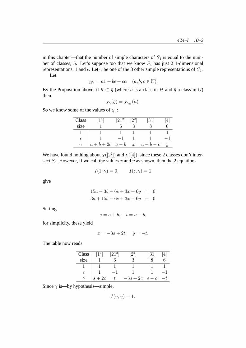
424–I 10–2

in this chapter—that the number of simple characters ofS4 is equal to the num-ber of classes, 5. Let’s suppose too that we knowS4 has just 2 1-dimensionalrepresentations,1 andε. Let γ be one of the 3 other simple representations ofS4.

LetγS3 = a1 + bε+ cα (a, b, c ∈ N).

By the Proposition above, ifh ⊂ g (whereh is a class inH and g a class inG)then

χγ(g) = χγH (h).

So we know some of the values ofχγ:

Class [14] [212] [22] [31] [4]size 1 6 3 8 61 1 1 1 1 1ε 1 −1 1 1 −1γ a+ b+ 2c a− b x a+ b− c y

We have found nothing aboutχ([22]) andχ([4]), since these 2 classes don’t inter-sectS3. However, if we call the valuesx andy as shown, then the 2 equations

I(1, γ) = 0, I(ε, γ) = 1

give

15a+ 3b− 6c+ 3x+ 6y = 0

3a+ 15b− 6c+ 3x+ 6y = 0

Settings = a+ b, t = a− b,

for simplicity, these yield

x = −3s+ 2t, y = −t.

The table now reads

Class [14] [212] [22] [31] [4]size 1 6 3 8 61 1 1 1 1 1ε 1 −1 1 1 −1γ s+ 2c t −3s+ 2c s− c −t

Sinceγ is—by hypothesis—simple,

I(γ, γ) = 1.

424–I 10–3

Thus24 = (s+ 2c)2 + 6t2 + 3(−3s+ 2c)2 + 8(s− c)2 + 6t2.

On simplification this becomes

2 = 3s2 − 4sc+ 2c2 + t2

= s2 + 2(s− c)2 + t2.

Noting thats, t, c are all integral, and thats, c ≥ 0, we see that there are just 3solutions to this diophantine equation:

(a, b, c) = (1, 0, 1), (0, 1, 1), (0, 0, 1).

These must yield the 3 missing characters.We have determined the character table ofS4 without constructing—even

implicitly—the corresponding representations. This has an interesting parallel inrecent mathematical history. One of the great achievements of the last 25 years hasbeenthe determination of all finite simple groups, ie groups possessing no propernormal (or self-conjugate) subgroups. The last link in the chain was the deter-mination of theexceptionalsimple groups, ie those not belonging to the knowninfinite families (such as the family of alternating groupsAn for n ≥ 5). Finally,all was known except for the largest exceptional group—the so-calledmammothgroup. The character table of this group had been determined several years beforeit was established that a group did indeed exist with this table.

As we remarked earlier, the technique above isnot recommended for seriouscharacter hunting. The method of choice must be induced representations, ournext topic.

SupposeV is a vector space. Then we denote byC(G, V ) theG-space ofmapsf : G→ V , with the action ofG defined by

(gf)(x) = f(g−1x)

(This extends our earlier definition ofC(G, k).)

Definition 10.2 SupposeH is a subgroup ofG; and supposeα is a representationofH in U . Then we define the induced representationαG ofG as follows. Let

V = {F ∈ C(G,U) : F (gh) = h−1F (g) for all g ∈ G, h ∈ H}.

ThenV is aG-subspace ofC(G,U); and αG is the representation ofG in thissubspace.

424–I 10–4

Remark:ThatV is aG-subspace follows from the fact that we are acting onGwithG andH from opposite sides (G on the left,H on the right); and their actionstherefore commute:

(gx)h = g(xh).

Thus ifF ∈ V then

(gF )(xh) = F (g−1xh)

= h−1F (g−1x)

= h−1((gF )(x)),

ie gF ∈ V .This definition is too cumbersome to be of much practical use. The following

result offers an alternative, and usually more convenient, starting point.

Lemma 10.1 Supposee = g1, g2, ..., gr are representatives of the cosets ofH inG, ie

G = g1H ∪ g2H ∪ ... ∪ grH.

Then there exists anH-subspaceU ′ ⊂ V such that

(a)U ′ is isomorphic toU as anH-space,

(b) V = g1U′⊕ g2U

′⊕ ...⊕grU

′.

Moreover the induced representationαG is uniquely characterised by the exis-tence of such a subspace.

Remarks:

1. After the lemma, we may write

V = g1U⊕

g2U⊕

...⊕

grU.

2. The action ofG onV is implicit in this description ofV . For supposev isin theith summand, say

v = giu;

and supposeggi is in thejth coset, say

ggi = gjh.

Thengv is in thejth summand:

gv = ggiu = gj(hu).

424–I 10–5

3. The difficulty of taking this result as the definition ofαG lies in the awk-wardness of showing that the resulting representation does not depend onthe choice of coset-representatives.

Proof I To eachu ∈ U let us associate the functionu′ = u′(g) ∈ C(G,U) by

u′(g) =

{gu if g ∈ H0 otherwise

Then it is readily verified that

(a) u′ ∈ V , ieu′(gh) = h−1u′(g) for all h ∈ H.

(b) If u 7→ u′ thenhu 7→ hu′.

Thus the mapu 7→ u′ sets up anH-isomorphism betweenU and anH-subspaceU ′ ⊂ V .

SupposeF ∈ V . From the definition ofV ,

F (gh) = h−1F (g).

It follows that the values ofF on any cosetgiH are completely determined by itsvalue at one pointgi. ThusF is completely determined by itsr values

u1 = F (e), u2 = F (g2), ..., ur = F (gr).

Let us writeF ←→ (u1, u2, ..., ur).

Then it is readily verified that

u′ ←→ (u, 0, ..., 0);

and more generallygiu′ ←→ (0, .., u, .., 0),

ie the functiongiu′ vanishes on all except theith cosetgiH, and takes the valueuatgi.

It follows thatF = g1u

′1 + g2u

′2 + . . .+ gru

′r

since the 2 functions take the same values at ther pointsgi. Moreover the argu-ment shows that this expression forF ∈ V as a sum of functions in the subspacesU ′ = g1U

′, g2U′, ..., grU

′, respectively, is unique: so that

V = g1U′⊕ g2U

′⊕ ...⊕

grU′.

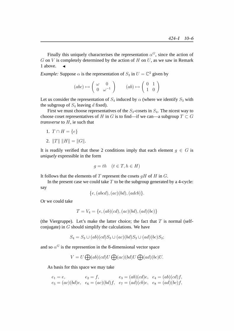
424–I 10–6

Finally this uniquely characterises the representationαG, since the action ofG onV is completely determined by the action ofH onU , as we saw in Remark1 above. J

Example:Supposeα is the representation ofS3 in U = C2 given by

(abc) 7→(ω 00 ω−1

)(ab) 7→

(0 11 0

)

Let us consider the representation ofS4 induced byα (where we identifyS3 withthe subgroup ofS4 leavingd fixed).

First we must choose representatives of theS3-cosets inS4. The nicest way tochoose coset representatives ofH in G is to find—if we can—a subgroupT ⊂ GtransversetoH, ie such that

1. T ∩H = {e}

2. ‖T‖ ‖H‖ = ‖G‖.

It is readily verified that these 2 conditions imply that each elementg ∈ G isuniquelyexpressible in the form

g = th (t ∈ T, h ∈ H)

It follows that the elements ofT represent the cosetsgH of H in G.In the present case we could takeT to be the subgroup generated by a 4-cycle:

say{e, (abcd), (ac)(bd), (adcb)}.

Or we could take

T = V4 = {e, (ab)(cd), (ac)(bd), (ad)(bc)}

(the Viergruppe). Let’s make the latter choice; the fact thatT is normal (self-conjugate) inG should simplify the calculations. We have

S4 = S3 ∪ (ab)(cd)S3 ∪ (ac)(bd)S3 ∪ (ad)(bc)S3;

and soαG is the represention in the 8-dimensional vector space

V = U⊕

(ab)(cd)U⊕

(ac)(bd)U⊕

(ad)(bc)U.

As basis for this space we may take

e1 = e, e2 = f, e3 = (ab)(cd)e, e4 = (ab)(cd)f,e5 = (ac)(bd)e, e6 = (ac)(bd)f, e7 = (ad)(cb)e, e8 = (ad)(bc)f,

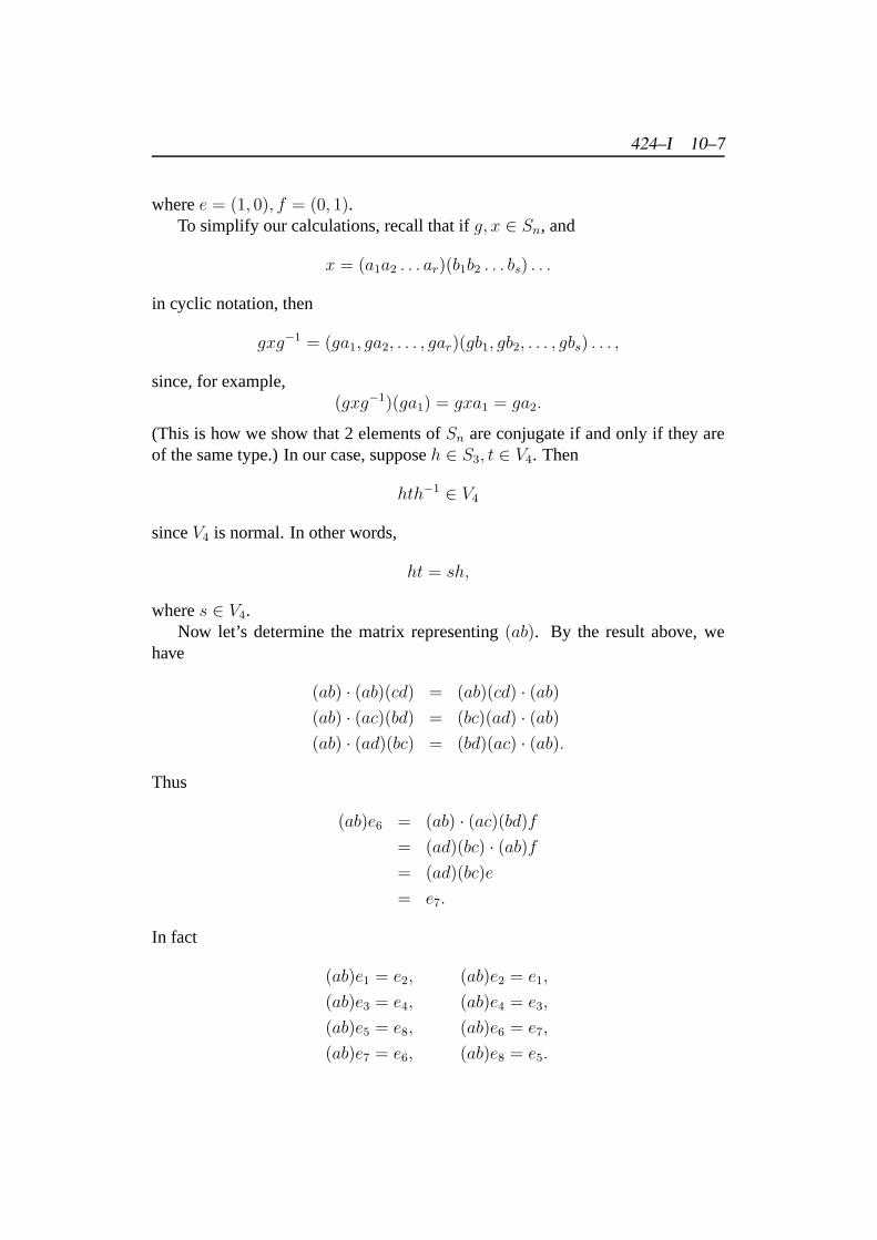
424–I 10–7

wheree = (1, 0), f = (0, 1).To simplify our calculations, recall that ifg, x ∈ Sn, and

x = (a1a2 . . . ar)(b1b2 . . . bs) . . .

in cyclic notation, then

gxg−1 = (ga1, ga2, . . . , gar)(gb1, gb2, . . . , gbs) . . . ,

since, for example,(gxg−1)(ga1) = gxa1 = ga2.

(This is how we show that 2 elements ofSn are conjugate if and only if they areof the same type.) In our case, supposeh ∈ S3, t ∈ V4. Then

hth−1 ∈ V4

sinceV4 is normal. In other words,

ht = sh,

wheres ∈ V4.Now let’s determine the matrix representing(ab). By the result above, we

have

(ab) · (ab)(cd) = (ab)(cd) · (ab)(ab) · (ac)(bd) = (bc)(ad) · (ab)(ab) · (ad)(bc) = (bd)(ac) · (ab).

Thus

(ab)e6 = (ab) · (ac)(bd)f

= (ad)(bc) · (ab)f= (ad)(bc)e

= e7.

In fact

(ab)e1 = e2, (ab)e2 = e1,

(ab)e3 = e4, (ab)e4 = e3,

(ab)e5 = e8, (ab)e6 = e7,

(ab)e7 = e6, (ab)e8 = e5.

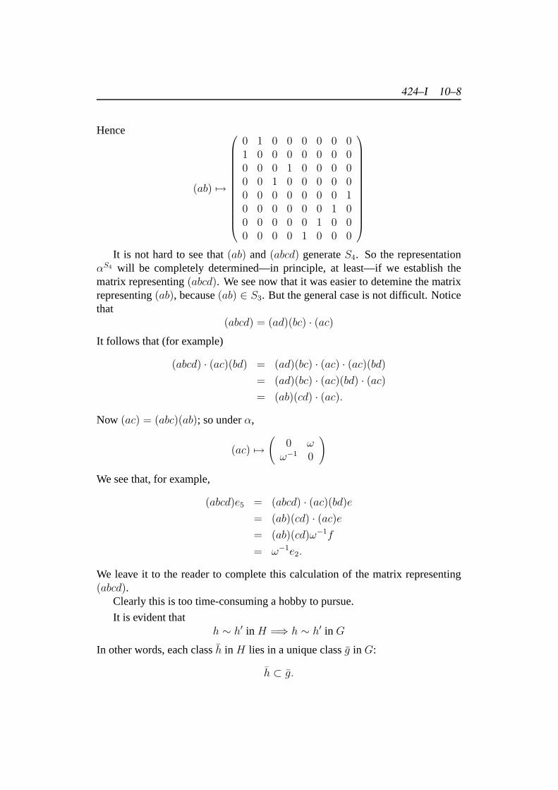
424–I 10–8

Hence

(ab) 7→

0 1 0 0 0 0 0 01 0 0 0 0 0 0 00 0 0 1 0 0 0 00 0 1 0 0 0 0 00 0 0 0 0 0 0 10 0 0 0 0 0 1 00 0 0 0 0 1 0 00 0 0 0 1 0 0 0

It is not hard to see that(ab) and(abcd) generateS4. So the representation

αS4 will be completely determined—in principle, at least—if we establish thematrix representing(abcd). We see now that it was easier to detemine the matrixrepresenting(ab), because(ab) ∈ S3. But the general case is not difficult. Noticethat

(abcd) = (ad)(bc) · (ac)It follows that (for example)

(abcd) · (ac)(bd) = (ad)(bc) · (ac) · (ac)(bd)

= (ad)(bc) · (ac)(bd) · (ac)= (ab)(cd) · (ac).

Now (ac) = (abc)(ab); so underα,

(ac) 7→(

0 ωω−1 0

)

We see that, for example,

(abcd)e5 = (abcd) · (ac)(bd)e

= (ab)(cd) · (ac)e= (ab)(cd)ω−1f

= ω−1e2.

We leave it to the reader to complete this calculation of the matrix representing(abcd).

Clearly this is too time-consuming a hobby to pursue.

It is evident thath ∼ h′ in H =⇒ h ∼ h′ in G

In other words, each classh in H lies in a unique classg in G:

h ⊂ g.

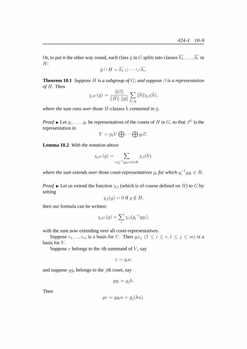
424–I 10–9

Or, to put it the other way round, each classg in G splitsinto classesh1, . . . , hr inH:

g ∩H = h1 ∪ · · · ∪ hr.

Theorem 10.1 SupposeH is a subgroup ofG; and supposeβ is a representationofH. Then

χβG(g) =‖G‖‖H‖ ‖g‖

∑h⊂g‖h‖χβ(h),

where the sum runs over thoseH-classesh contained ing.

Proof I Let g1, . . . , gr be representatives of the cosets ofH inG, so thatβG is therepresentation in

V = g1U⊕· · ·

⊕grU.

Lemma 10.2 With the notation above

χβG(g) =∑

i:g−1i ggi=h∈H

χβ(h),

where the sum extends over those coset-representativesgi for whichg−1i ggi ∈ H.

Proof I Let us extend the functionχβ (which is of course defined onH) toG bysetting

χβ(g) = 0 if g /∈ H,

then our formula can be written:

χβG(g) =∑i

χβ(g−1i ggi),

with the sum now extending over all coset-representatives.Supposee1, ..., em is a basis forU . Thengiej (1 ≤ i ≤ r, 1 ≤ j ≤ m) is a

basis forV .Supposev belongs to theith summand ofV , say

v = giu;

and supposeggi belongs to thejth coset, say

ggi = gjh.

Thengv = ggiu = gj(hu).

424–I 10–10

Sog(giU) ⊂ gjU.

Thus the basis elements ingiU cannot contribute toχβG(g) unlessi = j, that is,unlessggi = gih, ie

g−1i ggi = h ∈ H.

Moreover if this is so theng(giej) = gi(hej),

ie them × m matrix defining the action ofg on giU with respect to the basisgie1, ..., giem is justB(h); so that its contribution toχβG(g) is

χβ(h).

The result follows on adding the contributions from all those summands sent intothemselves byg. J

Lemma 10.3 For eachg ∈ G,

χβG(g) =1

‖H‖∑

g′∈G:g′−1gg′=h∈H

χβ(h)

Proof I Suppose we take a different representative of theith coset, say

g′i = gih.

This will make the same contribution to the sum, since

g′i−1gg′i = h−1(g−1

i ggi)h;

andχβ(h−1h′h) = χβ(h′).

Thus if we sum over all the elements ofG, we shall get each coset-contributionjust‖H‖ times. J

To return to the proof of the Proposition, we compute how many times eachelementh ∈ H occurs in the sum above.

Two elementsg′, g′′ define the same conjugate ofg in G, ie

g′−1gg′ = g′′

−1gg′′,

if and only if g′′g′−1 andg commute, ie if and only

g′′N(g) = g′N(g),

424–I 10–11

whereN(g) = {x ∈ G : gx = xg}.

It follows that eachG-conjugateh of g in H will occur just‖N(g)‖ times in thesum of Corollary 1. Thus if we sum over these elementsh we must multiply by‖N(g)‖.

The result follows, since

|N(g)‖ =‖G‖‖g‖

by the same argument, each conjugatex−1gx of g arising from‖N(g)‖ elementsx. J

Examples:

1. Let us look again atαS3→S4 . The classes ofS4 andS3 are related as follows:

[14] ∩ S3 = [13]

[212] ∩ S3 = [21]

[22] ∩ S3 = ∅[31] ∩ S3 = [3]

[4] ∩ S3 = ∅

Hence

χαS4 ([14]) =24

6 · 1χα(13) = 8

χαS4 ([212]) =24

6 · 63χα(21) = 0

χαS4 ([22]) = 0

χαS4 ([31]) =24

6 · 82χα(3) = −1

χαS4 (4) = 0

Class [14] [212] [22] [31] [4]size 1 6 3 8 6αS4 8 0 0 −1 0

Since

I(αS4 , αS4) =1

24

(82 + 8 · 12

)= 3,

424–I 10–12

αS4 has just 3 distinct simple parts. whose determination is left to the reader.

The relation betweenS4 andS3 is unusual, in thatclasses never split. If gis a class inS4 theng ∩ S3 is either a whole classh in H, or else is empty.This is true more generally forSn andSm (m < n), whereSm is identifiedwith the subgroup ofSn leaving the lastn−m elements fixed. Ifg is a classin Sn, then

g ∩ Sm = h or ∅.

2. Now let’s look at the cyclic subgroup

C4 = 〈(abcd)〉 = {e, (abcd), (ac)(bd), (adcb)}

of S4. SinceC4 is abelian, each element is in a class by itself. Letθ be the1-dimensional representation ofC4 defined by

(abcd) 7→ i

We have

[14] ∩ C4 = {e}[212] ∩ C4 = ∅[22] ∩ C4 = {(ac)(bd)}[31] ∩ C4 = ∅[4] ∩ C4 = {(abcd), (adcb)}

Hence

χθS4 ([14]) =24

4 · 1χθ(e) = 6

χθS4 ([212]) = 0

χθS4 ([22]) =24

4 · 3χθ((ac)(bd)) = −2

χθS4 ([31]) = 0

χθS4 ([4]) =24

4 · 6(χθ((abcd)) + χθ((adcb)))

= i+ (−i) = 0

Class [14] [212] [22] [31] [4]size 1 6 3 8 6θS4 6 −2 0 0 0

424–I 10–13

Since

I(θS4 , θS4) =1

24

(62 + 6 · 22

)= 3,

θS4 has just 3 distinct simple parts. whose elucidation we again leave to thereader.

Proposition 10.2 1. (α + α′)G = αG + α′G;

2. (α∗)G = (αG)∗;

3. dimαG = [G : H] dimα.

It is worth noting that permutation representations are a particular case of in-duced representations.

Lemma 10.4 SupposeG acts transitively on the finite setX. Letα be the corre-sponding representation ofG. Takex ∈ X; and let

Sx = {g ∈ G : gx = x}

be the corresponding stabilizer subgroup. Then

α = 1Sx→G,

ie α is the representation ofG obtained by induction from the trivial representa-tion ofSx.

Remark:The result is easily extended to non-transitive actions. For in that case theset splits into a number of orbits, on each of whichG acts transitively. On applyingthe Proposition to each orbit, we conclude that any permutation representation canbe expressed as a sum of representations, each of which arises by induction fromthe trivial representation of some subgroup ofG.

Proof I By Definition 1,α′ = 1Sx→G

is the representation in the subspace

V ⊂ C(G)

consisting of those functionsF : G→ k satisfying

F (gh) = h−1F (g) ∀h ∈ Sx.

424–I 10–14

But sinceSx acts trivially onk this condition reduces to

F (gh) = F (g),

ie F is constant on each cosetgSx. ThusV can be identified with the spaceC(G/Sx, k) of functions on the setG/Sx of Sx-cosets inG.

On the other hand, theG-setsX andG/Sx can be identified, with the elementgx ∈ X corresponding to the cosetgSx. Thus

C(G/Sx, k) = C(X, k).

Sinceα is by definition the representation ofG in CX the result follows. J

Proof I (Alternative) By Proposition 2,

χα′(g) = ‖{i : g−1i ggi ∈ Sx}‖

= ‖{i : ggix = gix}‖= ‖{y ∈ X : gy = y}‖,

since eachy ∈ X is uniquely expressible in the formy = gix. But by Proposition???,

χα(g) = ‖{y ∈ X : gy = y}‖.

Thusχα = χα′ ,

and soα = α′ = 1Sx→G.

J

Induced representations are of great practical value. But we end with an ex-tremely important theoretical application.

Proposition 10.3 The number of simple representations of a finite groupG isequal to the number of conjugacy classes inG.

Proof I Let s denote the number of classes inG. We already know that

• The characters ofG are class functions.

• The simple characters are linearly independent.

424–I 10–15

ThusG has at mosts simple characters; and the result will follow if we can showthat every class function is a linear combination of characters.

It suffices for the latter to show that we can find a linear combination of char-acters taking the value 1 on a given classg, and vanishing on all other classes.

We can extend the formula in the Theorem above to define a map

f(h) 7→ fG(g) : X(H, k)→ X(G, k)

from the spaceX(H, k) of class functions on the subgroupH ⊂ G to the spaceX(G, k) of class functions onG, by

fG(g) =‖G‖‖H‖‖g‖

∑h⊂g‖h‖f(h).

Evidently this map is linear:

F (h) = af(h) + bg(h) =⇒ FG(g) = afG(g) + bfG(g).

Choose anyg ∈ g. LetH be the subgroup generated byg. Thus ifg is of orderd,

H = Cd = 〈g〉 = {e, g, g2, . . . , gd−1}.

Let θ denote the 1-dimensional character onH defined by

θ(g) = ω = e2πi/d.

SinceH is abelian, each element is in a class by itself, so all functions onH areclass functions. Thed characters onH are

1, θ, θ2, . . . , θd−1.

Let f(h) denote the linear combination

f = 1 + ω−1θ + ω−2θ2 + · · ·+ ω−(d−1)θd−1.

Then

f(hi) =

{d if i = 1,0 if i = 0.

,

ie f vanishes off theH-class{g}, but is not identically 0.It follows that the induced functionfG(g) has the required property; it van-

ishes offg, while

fG(g) =‖G‖d‖H‖‖g‖

6= 0.

424–I 10–16

This proves the result, sincefG is a linear combination of characters:

fG = 1G + ωθG + ω2(θ2)G + · · ·+ ω−(d−1)(θd−1)G.

J

Examples:

1. S3 has 3 classes:13, 21 and3. So it has 3 simple representations overC, asof course we already knew: namely 1,ε andα.

2. D(4) has 5 classes:{e}, {s2}, {s, s3}, {c, d} and{h, v}. So it has 5 simplerepresentations overC. We already know of 4 1-dimensional representa-tions. In addition the matrices defining the natural 2-dimensional represen-tation inR2 also define a 2-dimensional complex representation. (We shallconsider this process of complexification more carefully in Chapter ???.)This representation must be simple, since the matrices do not commute, asthey would if it were the sum of 2 1-dimensional representations. Thus allthe representations ofD4 are accounted for.

Proposition 10.4 (Frobenius’ Reciprocity Theorem) Supposeα is a representa-tion ofG, andβ a representation ofH ⊂ G. Then

IG(α, βG) = IH(αH , β).

Proof IWe have

IG(α, βG) =1

‖G‖∑g

‖g‖χα(g)‖G‖‖H‖‖g‖

∑h⊂g‖h‖χβ(h)

=1

‖H‖∑h

‖h‖χα(h)χβ(h)

= IH(αH , β).

J

This short proof does not explainwhyFrobenius’ Reciprocity Theorem holds.For that we must take a brief excursion into category theory.

Let CG denote the category ofG-spaces andG-maps. Then restriction andinduction definefunctors

S : CG → CH , , I : CH → CG.

Now 2 functorsE : C1 → C2, F : C2 → C1

424–I 10–17

are said to beadjoint if for any 2 objectsX ∈ C1, Y ∈ C2 there are bijections

MC1(X,FY ) =MC2(EX, Y )

which are natural in the sense that given any morphism

f : X → X ′

in C1 the diagramM(X,FY ) ←− M(X ′, FY )∥∥∥∥ ∥∥∥∥M(EX, Y ) ←− M(EX ′, Y )

is commutative, and similarly given any morphism

e : Y → Y ′

in C2 the diagramM(X,FY ) −→ M(X,FY ′)∥∥∥∥ ∥∥∥∥M(EX, Y ) −→ M(EX, Y ′)

is commutative.It’s not difficult to establish—but would take us too far out of our way—that

the induction and restriction functors are adjointin this sense: ifV is aG-space,andU aH-space, then

homH(VH , U) = homG(V, UG).

On taking dimensions, this gives Frobenius’ Theorem:

IH(αH , β) = IG(α, βG).

Chapter 11

Representations of Product Groups

The representations of a product groupG×H can be expressed—in as neata way as one could wish—in terms of the representations ofG andH.

Definition 11.1 Supposeα is a representation ofG in the vector spaceU overk,and β a representation ofH in the vector spaceV over k. Then we denote byα×β the representation of the product groupG×H in the tensor productU ⊗Vdefined by

(g, h)∑

u⊗ v =∑

gu⊗ hv.

Lemma 11.1 1. χα×β(g, h) = χα(g)χβ(h)

2. dim(α× β) = dimα dim β

3. if α andβ are both representations ofG then

(α× β)G = αβ,

where the restriction is to the diagonal subgroup

G = {(g, g) : g ∈ G} ⊂ G×G.

Proposition 11.1 The representationα×β ofG×H overC is simple if and onlyif α andβ are both simple. Moreover, every simple representation ofG×H is ofthis form.

Proof I

Lemma 11.2 If α1, α2 are representations ofG, andβ1, β2 are representations ofH, all overk, then

I(α1 × β1, α2 × β2) = I(α1, β1)I(α2, β2)

424–I 11–1

424–I 11–2

Proof IWe have

I(α1 × β1, α2 × β2) =1

|G||H|∑

(g,h)∈G×Hχα1×β1(g, h)χα2×β2(g, h)

=1

|G||H|∑

(g,h)∈G×Hχα1(g)χβ1(h)χα2(g)χβ2(h)

=1

|G|∑g∈G

χα1(g)χα2(g)1

|G|∑h∈H

χβ1(h)χβ2(h)

= I(α1, β1)I(α2, β2)

J

Recall that a representationα overC is simple if and only if

I(α, α) = 1.

Thus ifα is a simple representation ofG andβ is a simple representation ofH (both overC) then

I(α× β, α× β) = I(α, α)I(β, β) = 1;

and thereforeα× β is simple.Now supposeG hasr classes andH hass classes. ThenG×H hasrs classes,

since(g, h) ∼ (g′, h′)⇐⇒ g ∼ g′ andh ∼ h′.

But we have just producedrs simple representationsα×β of G×G; so these arein fact the full complement.

(The lemma shows that these representations are distinct; for

I(α1 × β1, α2 × β1) = I(α1, α2)I(β1, β2) = 0

unlessα1 = α2 andβ1 = β2.) J

It is useful to give a proof of the last part of the Proposition not using the fun-damental result that the number of simple representations is equal to the numberof classes; for we can give an alternative proof of this result using product groups.

Proof I (of last part of Proposition). Supposeγ is a representation ofG × H inW overC.

Consider the restrictionγH of γ to the subgroupH = e×H ⊂ G×H. LetVbe a simple part ofWH :

WH = V ⊕ · · ·Let

X = homH(V,W )

424–I 11–3

be the vector space formed by theH-mapst : V → W . This is non-trivial sinceV is a subspace ofW .

NowX is aG-space, under the action

(gt)(v) = g(tv)

LetU be a simpleG-subspace ofX. Then

homG(U,X) = homG(U,homH(V,W ))

= homG×H(U ⊗ V,W ).

Since this space is non-trivial, there exists aG×H map

θ : U ⊗ V → W.

But since bothU ⊗ V andW are simple, we must have

ker θ = 0, im θ = W.

Henceθ is an isomorphism, ie

W = U ⊗ V.

Thusγ = α× β,

whereα is the representation ofG in U , andβ is the representation ofH in V .J

Theorem 11.1 SupposeG hasn elements ands classes. Then

1. G hass simple representations overC;

2. if these areσ1, . . . , σs then

dim2 σ1 + · · ·+ dim2 σs = n.

Proof I Let τ be the permutation representation ofG×G in C(G, k) induced bythe action

(g, h)x = gxh−1

of G×G onG.

Lemma 11.3 The character ofτ is given by

χτ (g, h) =

{|G|/|g| if g ∼ h0 otherwise

424–I 11–4

Proof I Sinceτ is a permutational representation,

χτ (g, h) = |{x : (g, h)x = x}|= |{x : gxh−1 = x}|= |{x : x−1gx = h}|.

If g 6∼ h then clearly no suchx exists.Supposeg ∼ h. Then there exists at least onex, sayx0, such that

h = x−10 gx0.

Now

x−1gx = h ⇐⇒ x−1gx = x−10 gx0

⇐⇒ (xx−10 )g = g(xx−1

0 )

⇐⇒ xx−10 ∈ Z(g)

⇐⇒ x ∈ Z(g)x0.

Thus

χτ (g, h) = |{x : gxh−1 = x|= |Z(g)|= |G|/|g|.

J

Lemma 11.4 SupposeG has simple representationsσ1, . . . σs. Then

τ = σ∗1 × σ1 + · · ·+ σ∗s × σs.

Proof IWe know that the simple representations ofG×G areσi × σj. Thus

τ =∑i,j

e(i, j)σi × σj,

wheree(i.j) ∈ N.

424–I 11–5

To determinee(i, j) we must compute the intertwining number

I(τ, σi × σj) =1

|G|2∑g,h

χτ (g, h)χσi×σj(g, h)

=1

|G|2∑g,h

χτ (g, h)χσi(g)χσj(h)

=1

|G|2∑h∼g

|G||g|

χσi(g)χσj(h)

=1

|G|χσi(g)χσj(g)

=1

|G|χσ∗i (g)χσj(g)

= I(σ∗i , σj).

Thus

I(τ, σi × σj) =

{1 if σ∗i = σj0 otherwise

In other words,σi × σj occurs inτ if and only if σ∗i = σj, and then occurs justonce. J

It follows from this result in particular that the number of simple representa-tions is equal toI(τ, τ).

Lemma 11.5 I(τ, τ) is equal to the number of classes inG.

Proof IWe have

I(τ, τ) =1

|G|2∑g,h

|χτ (g, h)|2

=1

|G|2∑g

∑h∼g

(|G||g|

)2

=1

|G|2∑g

|g| |G|2

|g|2

=∑g

1

|g|.

Since each class contributes|g| terms to this sum, each equal to1/|g|, the sum isequal to the number of classes.J

That proves the first part of the Theorem; the number of simple representationsis equal toI(τ, τ), which in turn is equal to the number of classes.

424–I 11–6

The second part follows at once on taking dimensions in

τ = σ∗1 × σ1 + · · ·+ σ∗s × σs.

J

Example:We can think of product groups in 2 ways—as a method of constructingnew groups, or as a way of splitting up a given group into factors.

We say thatG = H ×K, whereH,K are subgroups ofG, if the map

H ×K → G : (h, k) 7→ hk

is an isomorphism.A necessary and sufficient condition for this— supposingG finite—is that

1. elements ofH andK commute, ie

hk = kh

for all h ∈ H, k ∈ K; and

2. |G| = |H||K|.

Now consider the symmetry groupG of a cube. This has 48 elements; forthere are 8 vertices, and 6 symmetries leaving a given vertex fixed.

Of these 48 symmetries, half are proper and half improper. The proper sym-metries form a subgroupP ⊂ G.

Let Z = {I, J}, whereJ denotes reflection in the centre of the cube. In factZ is the centre ofG:

Z = ZG = {z ∈ G : zg = gz for all g ∈ G}.

By the criterion above,G = Z × P.

Moreover,P = S4,

as we can see by considering the action of symmetries on the 4 diagonals of thecube. This defines a homomorphism

Θ : P → S4.

Since no symmetry send every diagonal into itself,

ker Θ = {I}.

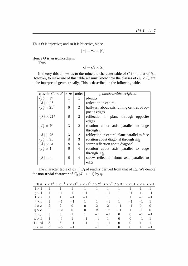
424–I 11–7

ThusΘ is injective; and so it is bijective, since

|P | = 24 = |S4|.

HenceΘ is an isomorphism.Thus

G = C2 × S4.

In theory this allows us to dtermine the character table ofG from that ofS4.However, to make use of this table we must know how the classes ofC2 × S4 areto be interpreted geometrically. This is described in the following table.

class inC2 × P size order geometricaldescription{I} × 14 1 1 identity{J} × 14 1 1 reflection in centre{I} × 212 6 2 half-turn about axis joining centres of op-

posite edges{J} × 212 6 2 relflection in plane through opposite

edges{I} × 22 3 2 rotation about axis parallel to edge

throughπ{J} × 22 3 2 relflection in central plane parallel to face{I} × 31 8 3 rotation about diagonal through±π

3

{J} × 31 8 6 screw reflection about diagonal{I} × 4 6 4 rotation about axis parallel to edge

through±π2

{J} × 4 6 4 screw reflection about axis parallel toedge

The character table ofC2 × S4 id readily derived from that ofS4. We denotethe non-trivial character ofC2 (J 7→ −1) by η.

Class I × 14 J × 14 I × 212 J × 212 I × 22 J × 22 I × 31 J × 31 I × 4 J × 41× 1 1 1 1 1 1 1 1 1 1 1η × 1 1 −1 1 −1 1 −1 1 −1 1 −11× ε 1 1 −1 −1 1 1 1 1 −1 −1η × ε 1 −1 −1 1 1 −1 1 −1 −1 11× α 2 2 0 0 2 2 −1 −1 0 0η × α 2 −2 0 0 2 −2 −1 1 0 01× β 3 3 1 1 −1 −1 0 0 −1 −1η × β 3 −3 1 −1 −1 1 0 0 −1 11× εβ 3 3 −1 −1 −1 −1 0 0 1 1η × εβ 3 −3 −1 1 −1 1 0 0 1 −1

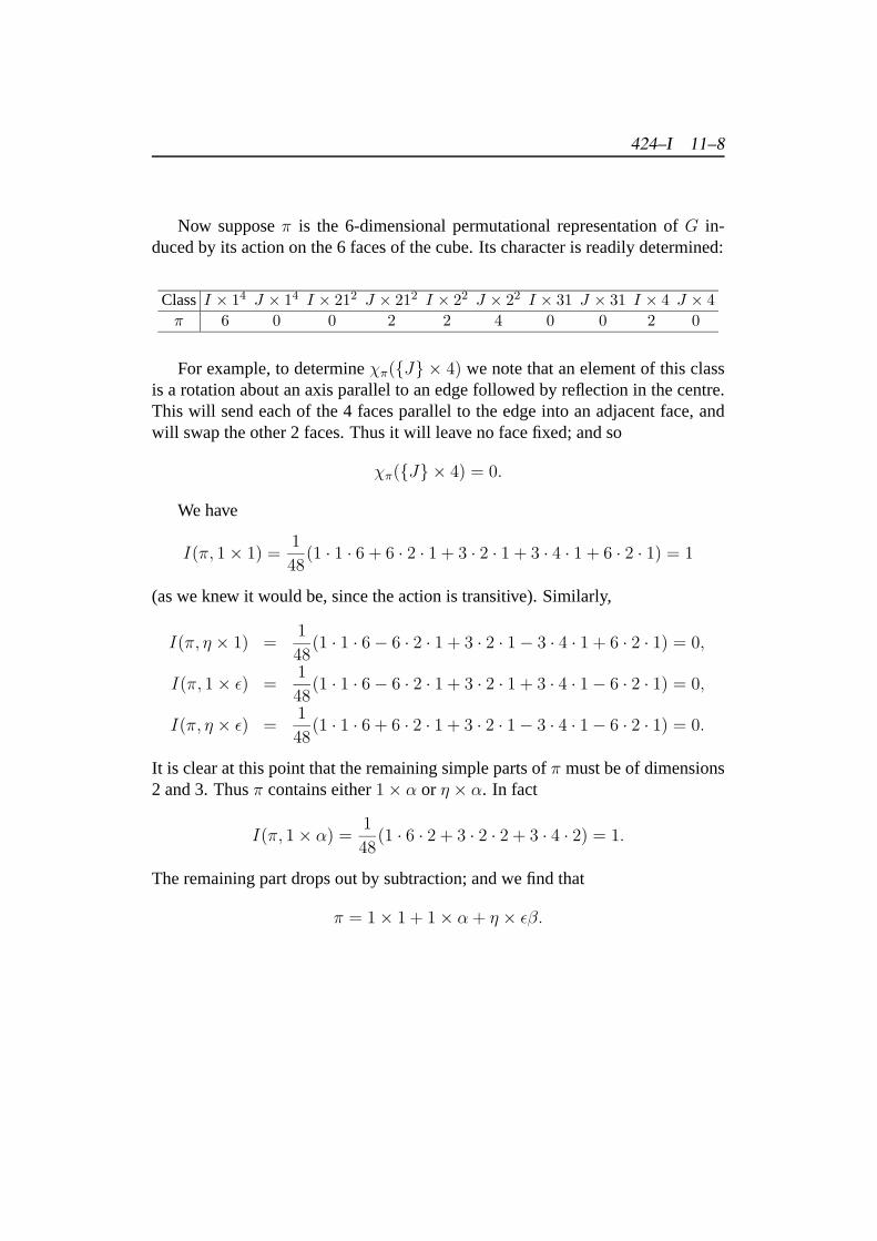
424–I 11–8

Now supposeπ is the 6-dimensional permutational representation ofG in-duced by its action on the 6 faces of the cube. Its character is readily determined:

ClassI × 14 J × 14 I × 212 J × 212 I × 22 J × 22 I × 31 J × 31 I × 4 J × 4π 6 0 0 2 2 4 0 0 2 0

For example, to determineχπ({J} × 4) we note that an element of this classis a rotation about an axis parallel to an edge followed by reflection in the centre.This will send each of the 4 faces parallel to the edge into an adjacent face, andwill swap the other 2 faces. Thus it will leave no face fixed; and so

χπ({J} × 4) = 0.

We have

I(π, 1× 1) =1

48(1 · 1 · 6 + 6 · 2 · 1 + 3 · 2 · 1 + 3 · 4 · 1 + 6 · 2 · 1) = 1

(as we knew it would be, since the action is transitive). Similarly,

I(π, η × 1) =1

48(1 · 1 · 6− 6 · 2 · 1 + 3 · 2 · 1− 3 · 4 · 1 + 6 · 2 · 1) = 0,

I(π, 1× ε) =1

48(1 · 1 · 6− 6 · 2 · 1 + 3 · 2 · 1 + 3 · 4 · 1− 6 · 2 · 1) = 0,

I(π, η × ε) =1

48(1 · 1 · 6 + 6 · 2 · 1 + 3 · 2 · 1− 3 · 4 · 1− 6 · 2 · 1) = 0.

It is clear at this point that the remaining simple parts ofπ must be of dimensions2 and 3. Thusπ contains either1× α or η × α. In fact

I(π, 1× α) =1

48(1 · 6 · 2 + 3 · 2 · 2 + 3 · 4 · 2) = 1.

The remaining part drops out by subtraction; and we find that

π = 1× 1 + 1× α + η × εβ.

Chapter 12

Exterior Products

12.1 The exterior products of a vector space

SupposeV is a vector space. Recall that itsrth exterior product∧rV is a vectorspace, spanned by elements of the form

v1 ∧ · · · ∧ vr (v1, . . . , vr ∈ V ),

wherevπ1 ∧ · · · ∧ vπr = ε(π)v1 ∧ · · · ∧ vr

for any permutationπ ∈ Sr.This implies in particular that any product containing a repeated element van-

ishes:· · · ∧ v ∧ · · · ∧ v ∧ · · · = 0.

(We are assuming here that the characteristic of the scalar fieldk is not 2. In factwe shall only be concerned with the casesk = R orC.)

The exterior product∧rV could be defined rigorously as the quotient-space

∧rV = V ⊗r/X,

whereX is the subspace ofV ⊗r spanned by all elements of the form

vπ1 ∧ . . . vπr − ε(π)v1 ∧ · · · ∧ vr,

wherev1, . . . , vr ∈ V, π ∈ Sr, andε denotes the parity representation ofSr.Supposee1, . . . , en is a basis forV . Then

ei1 ∧ ei2 ∧ · · · ∧ eir (i1 < i2 < · · · < ir)

424–I 12–1

12.1. THE EXTERIOR PRODUCTS OF A VECTOR SPACE 424–I 12–2

is a basis for∧rV . (Note that there is one basis element corresponding to eachsubset of{e1, . . . , en} containingr elements.) It follows that ifdimV = n then

∧rV = 0 if r > n;

while if r ≤ n then

dim∧rV =

(n

r

).

Now supposeT : V → V is a linear map. Then we can define a linear map

∧rT : ∧rV → ∧rV

by(∧rT )(v1 ∧ · · · ∧ vr) = (Tv1) ∧ · · · ∧ (Tvr).

(To see that this action is properly defined, it is sufficient to see that it sends thesubspaceX ⊂ V ⊗n described above into itself; and that follows at once since

(∧rT ) (vπ1 ∧ · · · ∧ vπr)−ε(π)v1∧. . . vr = (Tvπ1)∧· · ·∧(Tvπr)−ε(π)(Tv1)∧· · ·∧(Tvr)

is again one of the spanning elements ofX.)In the caser = n, ∧nV is 1-dimensional, with the basis element

e1 ∧ · · · ∧ en;

and∧nT = (detT )I.

This is in fact the “true” definition of the determinant.Although we shall not make use of this, the spaces∧rV can be combined to

form theexterior algebra∧V of V

∧V =⊕∧rV,

with the “wedge multiplication”

∧ : ∧rV × ∧sV → ∧r+sV

defined by

(u1 ∧ · · · ∧ ur) ∧ (v1 ∧ · · · ∧ vs) = u1 ∧ · · · ∧ ur ∧ v1 ∧ · · · ∧ vs,

extended to∧V by linearity.Observe that ifa ∈ ∧rV, b ∈ ∧sV then

b ∧ a = (−1)rsa ∧ b.

In particular the elements of even order form acommutativesubalgebra of∧V .

12.2. THE EXTERIOR PRODUCTS OF A GROUP REPRESENTATION424–I 12–3

12.2 The exterior products of a group representa-tion

Definition 12.1 Supposeα is a representation ofG in V . Then we denote by∧rαthe representation ofG in ∧rV defined by

g(v1 ∧ · · · ∧ vr) = (gv1) ∧ · · · ∧ (gvr).

In other words,g acts through the linear map∧r (α(g)).

Proposition 12.1 Supposeg ∈ G has eigenvaluesλ1, . . . , λn in the representa-tion α. Then the character of∧rα is therth symmetric sum of theλ’s, ie

χ∧rα(g) =∑

i1<i2<···<irλi1λi2 . . . λir .

Proof I Let us suppose thatk = C. We know thatα(g) can be diagonalised, iewe can find a basise1, . . . , en of the representation-spaceV such that

gei = λiei (i = 1, . . . , n).

But now

gei1 ∧ ei2 ∧ · · · ∧ eir = λi1λi2 . . . λi1ei1 ∧ ei2 ∧ · · · ∧ eir ,

from which the result follows, since these products form a basis for∧rV . J

12.3 Symmetric polynomials

We usually denote the symmetric product in the Proposition above by∑λ1 . . . λr.

It is an example of asymmetric polynomialin λ1, . . . , λn.More generally, supposeA is a commutative ring, with 1. (In fact we shall

only be interested in the ringsZ andQ.) As usual,A[x1, . . . , xn] denotes the ringof polynomials inx1, . . . , xn with coefficients inA.

The symmetric groupSn acts on this ring, by permutation of the variables:

(πP )(x1, . . . , xn) = P(xπ−1(1), . . . , xπ−1(n)

)(π ∈ Sn).

The polynomialP (x1, . . . , xn) is said to besymmetricif it is left invariant by thisaction ofSn. The symmetric polynomials evidently form asub-ringofA[x1, . . . , xn],which we shall denote byΣn(A).

12.3. SYMMETRIC POLYNOMIALS 424–I 12–4

Then polynomials

a1 =∑

xi, a2 =∑i1<i2

xi1xi2 , . . . , an = x1 · · ·xn

are symmetric; as are

s1 =∑

xi, s2 =∑

x2i , ; s3 =

∑x3i , . . . .

Proposition 12.2 The ringΣZ(n) is freely generated overZ bya1, . . . , an, ie themap

p(x1, . . . , xn) 7→ p(a1, . . . , an) : Z[x1, . . . , xn]→ Σn(Z)

is a ring-isomorphism.

Proof IWe have to show that

1. Every symmetric polynomialP (x1, . . . , xn) overZ (ie with integer coeffi-cients) is expressible as a polynomial ina1, . . . , an overZ:

P (x1, . . . , xn) = p(a1, . . . , an).

This will show that the map is surjective.

2. The map is injective, ie

p(a1, . . . , an) ≡ 0 =⇒ p ≡ 0.

1. Any polynomial is a linear combination ofmonomialsxe11 · · ·xenn . We orderthe monomials first by degree, with higher degree first, and then within eachdegreelexicographically, eg ifn = 2 then

1 < x2 < x1 < x22 < x1x2 < x2

1 < x32 < · · · .

The leading termin p(x1, . . . , xn) is the non-zero termcxe11 · · ·xenn contain-ing the greatest monomial in this ordering.

Now suppose the polynomialP (x1, . . . , xn) is symmetric. Evidentlye1 ≥e2 ≥ · · · ≥ en in the leading term. For if saye1 < e2 then the termcxe21 x

e12 · · ·xenn — which must also appear inP (x1, . . . , xn).

J

Corollary 12.1 The ringΣQ(n) is freely generated overQ bya1, . . . , an,

Proposition 12.3 The ringΣQ(n) is freely generated overQ bys1, . . . , sn,

Proof I J

12.4. NEWTON’S FORMULA 424–I 12–5

12.4 Newton’s formula

It follows from the Propositions above that the power-sumssn are expressible interms of the symmetric productsan, and vice versa. More precisely, there existpolynomialsSn(x1, . . . , xn) andAn(x1, . . . , xn) such that

sn = Sn(a1, . . . , n), an = An(a1, . . . , n),

with the coefficients ofSn integral and those ofAn rational. Newton’s formulaallows these polynomials to be determined recursively.

Let

f(t) = (1− x1t) · · · (1− xnt)= 1− a1t+ a2t

2 − · · ·+ (−1)nantn.

Then

f ′(t)

f(t)= frac−x11− x1t+ · · ·+ frac−xn1− xnt

= −s1 − s2t− s3t2 − · · · .

Thus

−a1+2a2t−3a3t2+· · ·+(−1)nnant

n−1 = (1−a1t+a2t2−· · ·+(−1)nant

n)(−s1−s2t−s3t2−· · · ).

Equating coefficients,

a1 = s1

2a2 = s1a1 − s2

3a3 = s1a2 − s2a1 + s3

. . .

rar = s1ar − s2ar−1 + · · ·+ (−1)r−1sr

. . .

Evidently these equations allow us to expresss1, s2, s3, . . . successively in

12.5. PLETHYSM 424–I 12–6

terms ofa1, a2, a3, . . . , or vice versa:

s1 = a1

s2 = a21 − 2a2

s3 = a31 − 3a1a2 + 3a3

. . .

a1 = s1

2a2 = s21 − s2

6a3 = s31 − 3s1s2 + 2s3

. . .

12.5 Plethysm

There is another way of looking at the exterior product — as a particular case oftheplethysmoperator on the representation-ringR(G).

SupposeV is a vector space over a fieldk of characteristic 0. (We shall onlybe interested in the casesk = R orC.) Then the symmetric groupSn acts on thetensor productV ⊗n by permutation of the factors:

π(v1 ⊗ · · · ⊗ vn) = vπ−11 ⊗ · · · ⊗ vπ−1n.

ThusV ⊗n carries a representation ofSn. As we know this splits into componentsV Σ corresponding to the simple representationsΣ of Sn:

V ⊗n = V Σ1 ⊕ · · · ⊕ V Σs ,

whereΣ1, . . . ,Σs are the simple representations ofSn. (We shall find it convenientto use superfixes rather than suffixes for objects corresponding to representationsof Sn.)

We are particularly interested in the components corresponding to the 2 1-dimensional representations ofSn: the trivial representation1n and the parityrepresentationεn, and we shall write

V P = V 1n , V N = V εn .

We also useP andN to denote the operations ofsymmetrisationandskew-symmetrisationonV ⊗n; that is, the linear maps

P,N : V ⊗n → V ⊗n

12.5. PLETHYSM 424–I 12–7

defined by

P (v1 ⊗ · · · ⊗ vn) =1

n!

∑π∈Sn

π(v1 ⊗ · · · ⊗ vn),

N(v1 ⊗ · · · ⊗ vn) =1

n!

∑π∈Sn

ε(π)π(v1 ⊗ · · · ⊗ vn).

Supposeπ ∈ Sn. Regardingπ as a mapV ⊗n → V ⊗n, we have

πP = P = Pπ, πN = ε(π)N = Nπ.

It follows that{P 2 = P, N2 = N,

ie P andN are bothprojectionsonto subspaces ofV ⊗n.We say thatx ∈ V ⊗n is symmetricif

πx = x

for all π ∈ Sn; and we say thatx is skew-symmetricif

πx = ε(π)x

for all π. It follows at once from the relationsπP = P, πN = εN that x issymmetric if and only if

Px = x;

while x is skew-symmetric if and only if

Nx = x.

ThusP is a projection onto the symmetric elements inV ⊗n, andN is a projectiononto the skew-symmetric elements.

To see the connection with the exterior product∧nV , recall that we coulddefine the latter by

∧nV = V ⊗n/X,

whereX ⊂ V ⊗n is the subspace spanned by elements of the form

πx− ε(π)x.

It is easy to see thatNx = 0 for such an elementx; while conversely, for anyx ∈ V ⊗n

x−Nx =1

n!

∑π∈Sn

ε(π) (ε(π)x− πxs)

∈ X

12.5. PLETHYSM 424–I 12–8

It follows thatX = kerN ;

and so (sinceN is a projection)

∧nV = V/X ∼= imN = V N ;

that is, thenth exterior product ofV can be identified with theε-component ofV ⊗n.

Now suppose thatV carries a representationα of some groupG. ThenG actsonV ⊗n through the representationαn.

Proposition 12.4 Supposeα is a represenation ofG in V . Then the actions ofGandSn onV ⊗n commute.

For each simple representationΣ of Sn, the componentV Σ of V ⊗n is stableunderG, and so carries a representationαΣ ofG. Thus

αn = αΣ1 + · · ·+ αΣs ,

whereΣ1, . . . ,Σs are the simple representations ofSn.

Proof IWe have

πg(v1 ⊗ · · · ⊗ vn) = π(gv1 ⊗ · · · ⊗ gvn)

= (gvπ−11 ⊗ · · · ⊗ gvπ−1n)

= gπ(v1 ⊗ · · · ⊗ vn).

J

Since the actions ofG andSn on V ⊗n commute, they combine to define arepresentation of the product groupG× Sn on this space.

Corollary 12.2 The representation ofG× Sn onV ⊗n is given by

αΣ1 × Σ1 + · · ·+ αΣs × Σs.

Supposeg ∈ G (or more accurately,α(g)) has eigenvaluesλ1, . . . , λd. Weknow that the character of

∧nα = αεn

is thenth symmetric product of theλi:

χ∧nα(g) = an(λ1, . . . , λd).

12.5. PLETHYSM 424–I 12–9

Proposition 12.5 To each simple representationΣ of Sn there corresponds aunique symmetric functionSΣ of degreen such that for any representationα ofG, and for anyg ∈ G with eigenvaluesλ1, . . . , λd,

χ∧nα(g) = SΣ(λ1, . . . , λd).

Proof IWe begin by establishing an important result which should perhaps havebeen proved when we discussed the splitting of aG-spaceV into components

V = Vσ1 ⊕ · · · ⊕ Vσs

corresponding to the simple representationsσ1, . . . , σs of G.

Lemma 12.1 The projectionPσ onto theσ-component ofV is given by

Pσ =dimσ

‖G‖∑g∈G

χσ(g−1)g.

Proof of LemmaB Supposeα is a representation ofG in V . Then the formula

above defines a linear mapP : V → V.

Supposeh ∈ G. Then (writingd for dimσ)

hPh−1 =d

‖G‖∑g

χσ(g−1)hgh−1

=d

‖G‖∑g′χσ(h−1g′

−1h)g′

=d

‖G‖∑g′χσ(g′

−1)g′

= P.

Now supposeα is simple. By Schur’s Lemma, the only linear transformationscommuting with allα(g) are multiples of the identity. Thus

P = ρI

for someρ ∈ C. Taking traces,

d

‖G‖∑g

χσ(g−1)χα(g) = ρd.

12.5. PLETHYSM 424–I 12–10

It follows that

ρ =

1 α = σ

0 α 6= σ

C In other words,

P =

I α = σ

0 α 6= σ

It follows thatP acts as the identity on all simpleG-subspaces carrying the repre-sentationσ, and as 0 on all simple subspaces carrying a representationσ′ 6= σ. Inparticular,P = I onVσ andP = 0 onVσ′ for all σ′ 6= σ. In other words,P is theprojection onto the componentVσ.

J

Chapter 13

Real Representations

Representation theory overC is much simpler than representation theoryoverR. For that reason, we usuallycomplexifyreal representations—extendthe scalars fromR toC—just as we do with polynomial equations. But at theend of the day we must determine if the representations—or solutions—thatwe have obtained are in fact real.

SupposeU is a vector space overR. Then we can define a vector spaceV =CU overC by “extension of scalars”. More precisely,

V = C⊗R U.

In practical terms,V = U ⊕ iU,

ie each elementv ∈ V is uniquely expressible in the form

v = u1 + iu2 (u1, u2 ∈ U).

If e1, . . . , en is a basis forU overR, then it is also a basis forV overC. Inparticular,

dimC V = dimR U.

On the other hand, supposeV is a vector space overC. Then we can define avector spaceU = RV overR by “forgetting” scalar multiplication by non-reals.Thus the elements ofU are precisely the same as those ofV . If e1, . . . , en is abasis forV over V , thene1, ie1, e2, ie2, . . . , en, ien is a basis forU overR. Inparticular,

dimR U = 2 dimC V.

Now supposeG acts on the vector spaceU overR. ThenG also acts onCU ,by

g(u1 + iu2) = (gu1) + i(gu2).

424–I 13–1

424–I 13–2

On the other hand, supposeG acts on the vector spaceV overC. ThenG alsoacts onRV by the same rule

(g, v) 7→ gv.

Definition 13.1 1. Supposeβ is a real representation ofG in U . Then wedenote byCβ the complex representation ofG in the vector space

CU = U ⊕ iU

derived fromU by extending the scalars fromR toC.

2. Supposeα is a complex representation ofG in V . Then we denote byRαthe real representation ofG in the vector spaceRV derived fromV by“forgetting” scalar multiplication by non-reals.

Remarks:

1. Supposeβ is described in matrix terms, by choosing a basis forU and givingthe matricesB(g) representingβ(g) with respect to this basis. Then we cantake the same basis forCU , and the same matrices to representCβ(g). Thusfrom the matrix point of view,β andCβ appear the same. The essentialdifference is thatCβ may split even ifβ is simple, ie we may be able to finda complex matrixP such that

PB(g)P−1 =

(C(g) 0

0 D(g)

)

for all g ∈ G, although no real matrixP has this property.

2. Supposeα is described in matrix form, by choosing a basise1, e2, . . . , enfor V , and giving the matricesA(g) representingα(g) with respect to thisbasis. Then we can take the2n elementse1, ie1, e2, ie2, . . . , en, ien as abasis forRV ; and the matrix representingRα(g) with respect to this basiscan be derived from the matrixA = A(g) representingα(g) as follows. Bydefinition,

ger =∑s

Asres.

LetAr,s = Xr,s + iYr,s,

whereXr,s, Yr,s ∈ R. Then

ger = Xsres + Ysries

g(ier) = −Ysres +Xsries

424–I 13–3

Thus the entryArs is replaced inRα(g) by the2× 2-matrix(Xr,s −Yr,sYr,s Xr,s

)

Proposition 13.1 1. C(β + β′) = Cβ + Cβ′

2. C(ββ′) = (Cβ)(Cβ′)

3. C(β∗) = (Cβ)∗

4. C1 = 1

5. dimCβ = dim β

6. χCβ(g) = χβ(g)

7. I(Cβ,Cβ′) = I(β, β′)

8. R(α + α′) = Rα + Rα′

9. R(α∗) = (Rα)∗

10. dimRα = 2 dimα

11. χRα(g) = 2<χα(g) = χα(g) + χα(g−1)

12. RCβ = 2β

13. CRα = α + α∗

Proof I All is immediate except (perhaps) parts (11) and (13).11. Supposeα(g) is represented by then× n matrix

A = X + iY,

whereX, Y are real. Then—as we saw above—the entryArs is replaced inRα(g)by the2× 2 matrix (

Xr,s −Yr,sYr,s Xr,s

)

424–I 13–4

Thus

trRα(g) = 2∑r

Xrr

= 2<(∑r

Arr)

= 2< trα(g)

= 2<χα(g)

= χα(g) + χα(g−1)

sinceχ(g) = χ(g−1).

13. This now follows on taking characters, since

χCRα(g) = χRα(g)

= χα(g) + χα(g−1)

= χα(g) + χα∗(g)

Since this holds for allg,CRα = α + α∗.

J

Lemma 13.1 Given a representationα ofG overC there exists at most one realrepresentationβ ofG overR such that

α = Cβ.

Proof I By Proposition 1,

Cβ = Cβ′ =⇒ χCβ(g) = χCβ′(g)

=⇒ χβ(g) = χβ′(g)

=⇒ β = β′.

J

Definition 13.2 A representationα of G overC is said to be real ifα = Cβ forsome representationβ overR.

Remarks:

424–I 13–5

1. In matrix termsα is real if we can find a complex matrixP such that thematrices

PB(g)P−1

are real for allg ∈ G.

2. Sinceβ is uniquely determined byα in this case, one can to some extentconfuse the two (as indeed in speaking ofα as real), although eg if dis-cussing simplicity it must be made clear whether the reference is toα or toβ.

Lemma 13.2 Consider the following 3 properties of the representationα overC:

1. α is real

2. χα is real, ieχα(g) ∈ R for all g ∈ G

3. α = α∗

We have(1) =⇒ (2)⇐⇒ (3).

Proof I (1) =⇒ (2): If α = Cβ then

χα(g) = χβ(g).

But the trace of a real matrix is necessarily real.(2)⇐⇒ (3): If χα is real then

χα(g) = χα(g) = χα∗(g)

for all g ∈ G. Henceα = α∗.

J

Problems involving representations overR often arise in classical physics,since the spaces there are normally real, eg those given by the electric and mag-netic fields, or the vibrations of a system. The best way of tackling such a problemis usually to complexify, ie to extend the scalars fromR toC. This allows the pow-erful techniques developed in the earlier chapters to be applied. But at the end ofthe day it may be necessary to determine whether or not the representations thatarise are real. The Lemma above gives a necessary condition: ifα is real thenits character must be real. But this condition is not sufficient; and our aim in therest of the Chapter is to find necessary and sufficient conditions for reality, of aspractical a nature as possible.

424–I 13–6

Definition 13.3 Supposeα is a simple representation overC. Then we say thatαis strictly complexif χα is not real; and we say thatα is quaternionicif χα is real,butα itself is not real;

Thus the simple representations ofG overC fall into 3 mutually exclusiveclasses:

R real: α = Cβ

C strictly complex:χα not real

H quaternionic:χα real butα not real

Lemma 13.3 Supposeα is a simple representation overC. Then

1. If α is real,Rα = 2β, whereβ is a simple representation overR;

2. if α is strictly complex or quaternionic,Rα = β is a simple representationoverR.

In particular, if χα is not real thenRα must be simple.

Proof I If α is real, sayα = Cβ, then by Proposition 1

Rα = RCβ = 2β.

Conversely, supposeRα splits, say

Rα = β + β′.

Then by Proposition 1,

α + α∗ = CRα = Cβ + Cβ′.

But sinceα andα∗ are simple, this implies (by the unique factorisation theorem)that

α = Cβ or α = Cβ′.

In either caseα is real. J

This gives a (not very practical) way of distinguishing between the 3 classes:

R: α real⇐⇒ χα real andRα splits

C: α quaternionic⇐⇒ χα real andRα simple

H: α strictly complex⇐⇒ χα not real (=⇒ Rα simple)

424–I 13–7

The next Proposition shows that the classification of simple representationsoverC into 3 classes leads to a similar classification of simple representationsoverR.

Proposition 13.2 Supposeβ is a simple representation overR. Then there are 3(mutually exclusive) possibilities:

R: Cβ = α is simple

C: Cβ = α + α∗,

H: Cβ = 2α, withα simple withα (andα∗) simple, andα 6= α∗

In case (R), α is real andI(β, β) = 1.

In case (C), α is strictly complex and

I(β, β) = 2.

In case (H), α is quaternionic and

I(β, β) = 4.

Proof I SinceRCβ = 2β,

Cβ cannot split into more than 2 parts. Thus there are 3 possibilities:

1. Cβ = α is simple

2. Cβ = 2α, with α simple

3. Cβ = α + α′, with α, α′ simple andα 6= α′

SinceI(β, β) = I(Cβ,Cβ)

by Proposition 1, the values ofI(β, β) in the 3 cases follow at once. Thus it onlyremains to show thatα is in the class specified in each case, and thatα′ = α∗ incase (3).

In case (1),α is real by definition.In case (2),

2χα(g) = χ2α(g) = χβ(g)

424–I 13–8

is real for allg ∈ G. Henceχα(g) is real, and soα is either real or quaternionic.If α were real, sayα = Cβ′, we should have

Cβ = 2Cβ′

which would imply thatβ = 2β′

by Proposition 2. Henceα is quaternionic.In case (3)

2β = RCβ = Rα + Rα′.

HenceRα = β = Rα′.

But thenα + α′ = Cβ = α + α∗.

Henceα′ = α∗.

Finally, sinceα∗ = α′ 6= α, α is strictly complex. J

Proposition 5 gives a practical criterion for determining which of the 3 classesa simple representationβ overR belongs to, namely by computingI(β, β) fromχβ. Unfortunately, the question that more often arises is: which class does a givensimple representationα overC belong to? and this is more difficult to determine.

Lemma 13.4 Supposeα is a simple representation ofG overC in V . Then

R: if α is real,there exists an invariant symmetric (quadratic) form onV , uniqueup to a scalar multiple—but there is no invariant skew-symmetric form onV ;

C: if α is complex, there is no invariant bilinear form onV .

H: if α is quaternionic, there exists an invariant skew-symmetric form onV ,unique up to a scalar multiple—but there is no invariant symmetric formonV ;

Proof I A bilinear form onV is a linear map

V ⊗ V → C,

ie an element of(V ⊗ V )∗ = V ∗ ⊗ V ∗.

424–I 13–9

Thus the space of bilinear maps carries the representation(α∗)2 of G. Hence theinvariant bilinear maps form a space of dimension

I(1, (α∗)2) = I(1, α∗α∗) = I(α, α∗)

Sinceα andα∗ are simple, this is 0 or 1 according asα = α∗ or not, ie accordingasα is either real or quaternionic, or strictly complex. In other words, ifα iscomplex there is no invariant bilinear form; while ifα is real or quaternionic thereis an invariant bilinear form onV , sayF (u, v), unique up to a scalar multiple.

Now any bilinear form can be split into a symmetric (or quadratic) part and askew-symmetric part; say

F (u, v) = Q(u, v) + S(u, v),

where

Q(u, v) =1

2(F (u, v) + F (v, u)) , S(u, v) =

1

2(F (u, v)− F (v, u))

But it is easy to see that ifF is invariant then so areQ andS. SinceF is the onlyinvariant bilinear form onV , it follows that either

F = Q or F = S,

ie F is either symmetric or skew-symmetric. It remains to show that the formeroccurs in the real case, the latter in the quaternionic case.

Supposeα is real, sayα = Cβ, whereβ is a representation in the real vectorspaceU . We know thatU carries an invariant symmetric form (in fact a positive-definite one), sayQ(u, u′). But this defines an invariant symmetric formCQ onV = CU by extension of scalars. So ifα is real,V carries an invariant symmetricform.

Finally, supposeα is quaternionic. ThenV carries either a symmetric or askew-symmetric invariant form (but not both). Suppose the former; sayQ(v, v′)is invariant. By Proposition 3,β = Rα is simple. Hence there exists a realinvariant positive-definite symmetric form onRV ; and this is the only invariantsymmetric form onRV , up to a scalar multiple. But the real part ofQ(v, v′) isalso an invariant form onRV ; and it is certainly not positive-definite, since

<Q(iv, iv) = −<Q(v, v).

This contradiction shows thatV cannot carry an invariant symmetric form. Weconclude that it must carry an invariant skew-symmetric form.J

We deduce from this Proposition the following more practical criterion forreality.

424–I 13–10

Proposition 13.3 Supposeα is a simple representation overC. Then

1

|G|∑g∈G

χα(g2) =

1 if α is real0 if α is strictly complex−1 if α is quaternionic

Proof I Every bilinear form has a unique expression as the sum of its symmetricand skew-symmetric parts. In other words, the space of bilinear forms is the directsum of the spaces of symmetric and of skew-symmetric forms; say

V ∗ ⊗ V ∗ = V Q ⊕ V S.

Moreover, each of these subspaces is stable underG; so the representation(α∗)2

in the space of bilinear forms splits in the same way; say

(α∗)2 = αQ + αS,

whereαQ is the representation ofG in the spaceV Q of symmetric forms on V,andαS is the representation in the spaceV S of skew-symmetric forms.

Now the dimensions of the spaces of invariant symmetric and skew-symmetricspace are

I(1, αQ) andI(1, αS),

respectively. Thus Proposition 6 can be reworded as follows:

R: If α is real thenI(1, αQ) = 1 andI(1, αS) = 0.

C: If α is complex then

I(1, αQ) = 0 andI(1, αS) = 0.

H: If α is quaternionic then

I(1, αQ) = 0 andI(1, αS) = 1.

Thus all (!) we have to do is to compute these 2 intertwining numbers. In factit suffices to find one of them, since

I(1, αQ) + I(1, αS) = I(1, (α∗)2) = I(α, α∗)

which we already know to be 1 ifα is real or quaternionic, and 0 ifα is complex.

424–I 13–11

To computeI(1, αQ), choose a basise1, ..., en for V ; and let the correspondingcoordinates bex1, ..., xn. Then then(n+ 1)/2 quadratic forms

x2i (1 ≤ i ≤ n), 2xixj (1 ≤ i < j ≤ n)

form a basis forV Q. Let gij denote the matrix defined byα(g). Thus if v =(x1, ..., xn) ∈ V , then the coordinates ofgv are

(gv)i =∑j

gijxj.

Henceg(x2

i ) =∑j,k

gijxjgikxk.

In particular, the coefficient ofx2i in this (which is all we need to know for the

trace) isg2ii. Similarly, the coefficient of2xixj in g(2xixj) is

giigjj + gijgji.

We conclude that

χαQ(g) =∑i

g2ii +

∑i,j:i<j

(giigjj + gijgji).

Butχα(g) =

∑i

gii, χα(g2) =∑i,j

gijgji.

Thus

χαQ(g) =1

2

(χα(g)2 + χα(g2)

).

Since

I(1, αQ) =1

|G|∑g∈G

χα[2](g),

it follows that

2I(1, αQ) =1

|G|∑g∈G

(χα(g))2 + χα(g2)

).

But1

|G|∑g

χα(g)2 = I(α, α∗).

Thus

2I(1, αQ) = I(α, α∗) +1

|G|∑g

χα(g2).

The result follows, sinceI(α, α∗) = 1 in the real and quaternionic cases, and 0 inthe complex case. J

Appendix A

Linear algebra over the quaternions

The basic ideas of linear algebra carry over with the quaternionsH (or in-deed any skew-field) in place ofR orC.

A vector spaceW overH is an abelian group (written additively) togetherwith an operation

H×W → W : (q, w) 7→ qw,

which we cann scalar multiplication, such that

1. q(w1 + w2) = qw1 + qw2,

2. (q1 + q2)w = q1w + q2w,

3. (q1q2)w = q1(q2w),

4. 1w = w.

The notions ofbasisanddimension(together withlinear independenceandspanning) carry over without change. Thuse1, . . . , en are said to be linearly inde-pendent if

q1e1 + · · ·+ qnen = 0 =⇒ q1 = · · · = qn = 0.

424–I 1–0