Ch9_Frequency Response Analysis
81
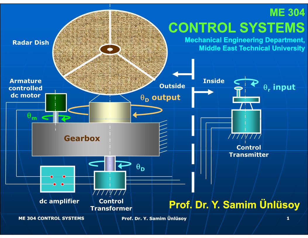
ME 304 ME 304 CONTROL SYSTEMS CONTROL SYSTEMS CONTROL SYSTEMS CONTROL SYSTEMS Mechanical Engineering Department, Mechanical Engineering Department, Middle East Technical University Middle East Technical University Radar Dish θ r input Armature controlled Outside Inside r controlled dc motor θ D output θ m Gearbox Control m Control Transmitter θ D Prof Dr Y Samim Ünlüsoy Prof Dr Y Samim Ünlüsoy Control dc amplifier ME 304 CONTROL SYSTEMS ME 304 CONTROL SYSTEMS Prof. Dr. Y. Samim Ünlüsoy Prof. Dr. Y. Samim Ünlüsoy 1 Prof. Dr . Y . Samim Ünlüsoy Prof. Dr . Y . Samim Ünlüsoy Transformer
Transcript of Ch9_Frequency Response Analysis
ME 304ME 304CONTROL SYSTEMSCONTROL SYSTEMSCONTROL SYSTEMSCONTROL SYSTEMS
Mechanical Engineering Department,Mechanical Engineering Department,Middle East Technical UniversityMiddle East Technical University
Radar Dish
θr inputArmature controlled Outside
Insider pcontrolled
dc motor θD output
θm
GearboxControl
m
Control Transmitter
θD
Prof Dr Y Samim ÜnlüsoyProf Dr Y Samim ÜnlüsoyControl dc amplifier
ME 304 CONTROL SYSTEMSME 304 CONTROL SYSTEMS Prof. Dr. Y. Samim ÜnlüsoyProf. Dr. Y. Samim Ünlüsoy 11
Prof. Dr. Y. Samim ÜnlüsoyProf. Dr. Y. Samim ÜnlüsoyTransformer
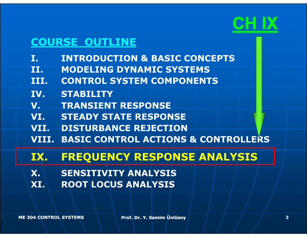
CH IXCH IXCOURSE OUTLINE
I. INTRODUCTION & BASIC CONCEPTSI. INTRODUCTION & BASIC CONCEPTSII. MODELING DYNAMIC SYSTEMSIII. CONTROL SYSTEM COMPONENTS
IV. STABILITYV. TRANSIENT RESPONSEVI. STEADY STATE RESPONSEVI. STEADY STATE RESPONSEVII. DISTURBANCE REJECTIONVIII. BASIC CONTROL ACTIONS & CONTROLLERS
IX. FREQUENCY RESPONSE ANALYSIS
X. SENSITIVITY ANALYSISX. SENSITIVITY ANALYSISXI. ROOT LOCUS ANALYSIS
ME 304 CONTROL SYSTEMSME 304 CONTROL SYSTEMS Prof. Dr. Y. Samim ÜnlüsoyProf. Dr. Y. Samim Ünlüsoy 22
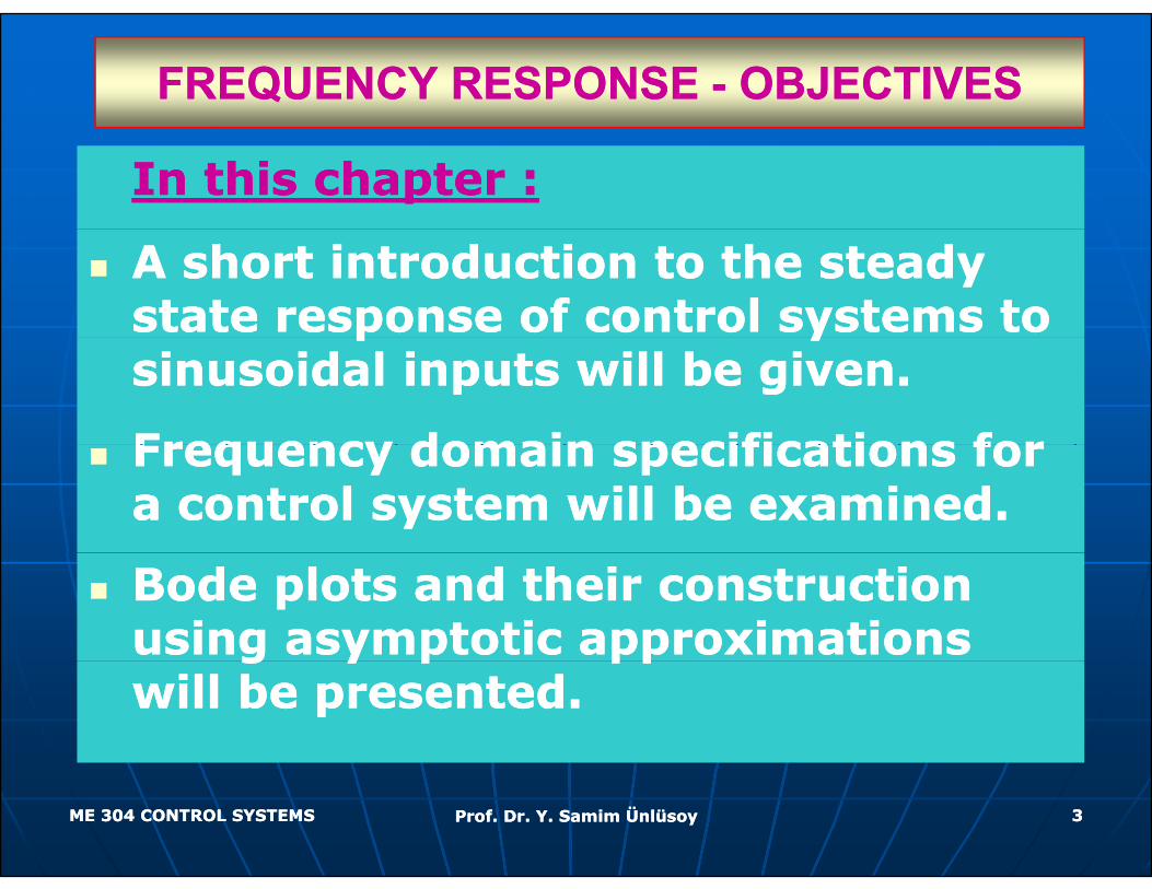
FREQUENCY RESPONSE FREQUENCY RESPONSE -- OBJECTIVESOBJECTIVES
In this chapter :In this chapter :
A short introduction to the steady A short introduction to the steady state response of control systems to state response of control systems to p yp ysinusoidal inputs will be given.sinusoidal inputs will be given.
Frequency domain specifications for Frequency domain specifications for Frequency domain specifications for Frequency domain specifications for a control system will be examined.a control system will be examined.
Bode plots and their construction Bode plots and their construction using asymptotic approximations using asymptotic approximations g y p ppg y p ppwill be presented. will be presented.
ME 304 CONTROL SYSTEMSME 304 CONTROL SYSTEMS Prof. Dr. Y. Samim ÜnlüsoyProf. Dr. Y. Samim Ünlüsoy 33
FREQUENCY RESPONSE FREQUENCY RESPONSE –– INTRODUCTIONINTRODUCTIONNi Ch 10Ni Ch 10Nise Ch. 10Nise Ch. 10
In frequency response analysis of control In frequency response analysis of control In frequency response analysis of control In frequency response analysis of control systems, systems, the steady state response of the the steady state response of the system to sinusoidal inputsystem to sinusoidal input is of interest.is of interest.
The frequency response analyses are The frequency response analyses are carried out in the carried out in the frequency domainfrequency domain, , q yq y ,,rather than the time domain.rather than the time domain.
It is to be noted that, It is to be noted that, time domain time domain It is to be noted that, It is to be noted that, time domain time domain properties of a control system can be properties of a control system can be predicted from its frequency domain predicted from its frequency domain characteristicscharacteristics..
ME 304 CONTROL SYSTEMSME 304 CONTROL SYSTEMS Prof. Dr. Y. Samim ÜnlüsoyProf. Dr. Y. Samim Ünlüsoy 44
FREQUENCY RESPONSE FREQUENCY RESPONSE -- INTRODUCTIONINTRODUCTION
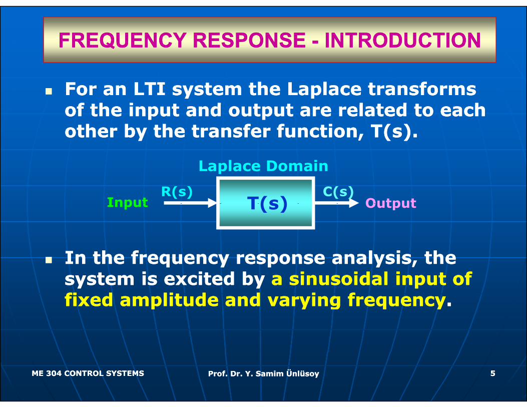
For an LTI system the Laplace transforms For an LTI system the Laplace transforms f th i t d t t l t d t h f th i t d t t l t d t h of the input and output are related to each of the input and output are related to each
other by the transfer function, T(s).other by the transfer function, T(s).
R(s) C(s)T(s)
Laplace Domain
Input Output
I th f l i th I th f l i th
T(s)Input Output
In the frequency response analysis, the In the frequency response analysis, the system is excited by system is excited by a sinusoidal input of a sinusoidal input of fixed amplitude and varying frequencyfixed amplitude and varying frequencyfixed amplitude and varying frequencyfixed amplitude and varying frequency..
ME 304 CONTROL SYSTEMSME 304 CONTROL SYSTEMS Prof. Dr. Y. Samim ÜnlüsoyProf. Dr. Y. Samim Ünlüsoy 55
FREQUENCY RESPONSE FREQUENCY RESPONSE -- INTRODUCTIONINTRODUCTION
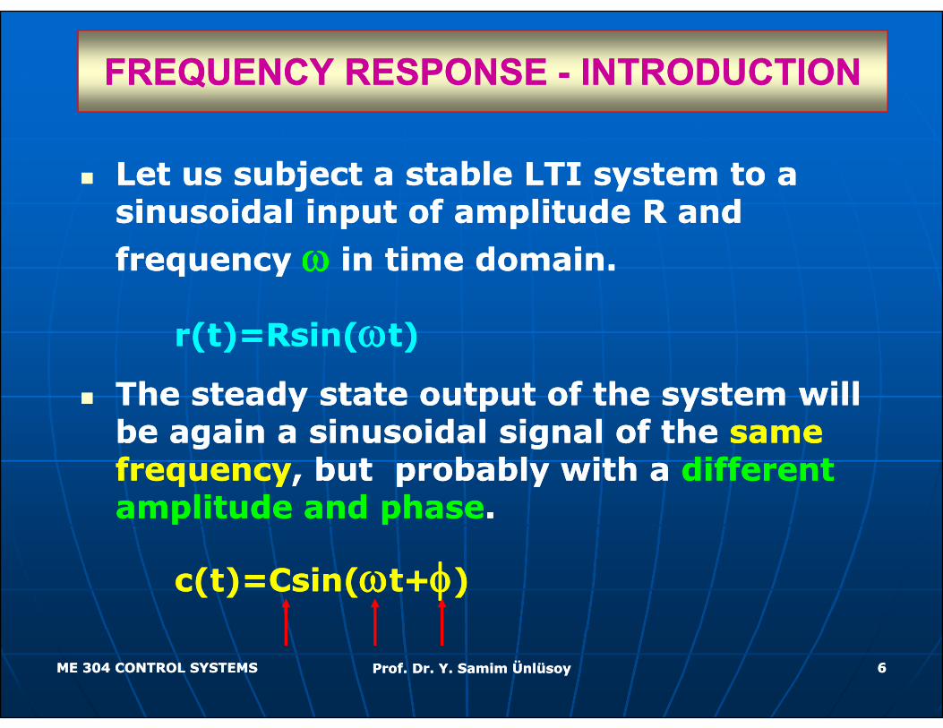
Let us subject a stable LTI system to a Let us subject a stable LTI system to a j yj ysinusoidal input of amplitude R and sinusoidal input of amplitude R and
frequency frequency ωω in time domain.in time domain.q yq y
r(t)=Rsin(r(t)=Rsin(ωωt)t)
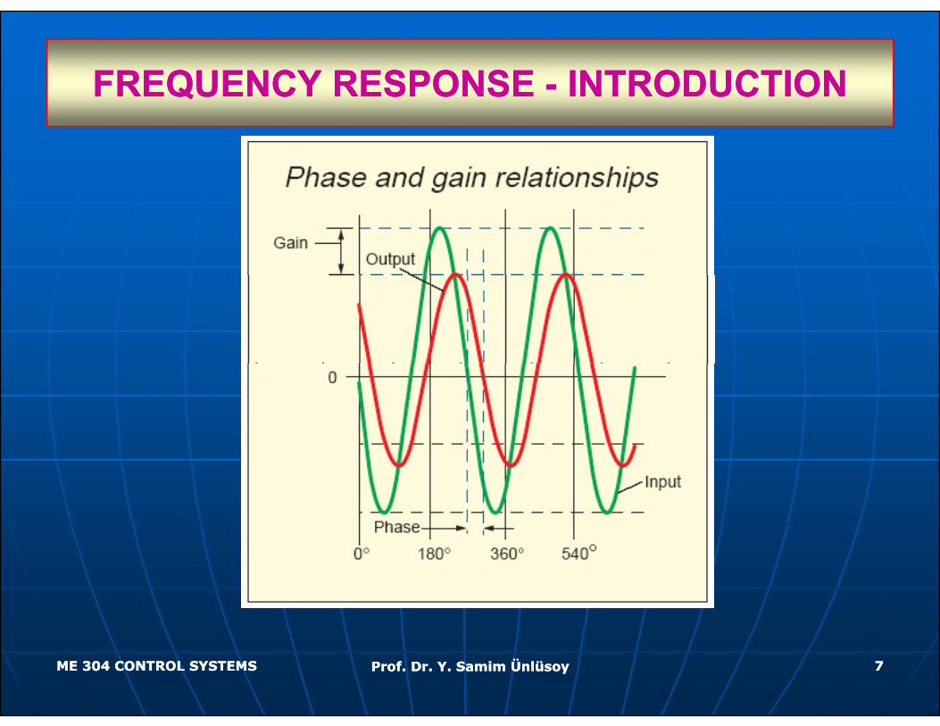
The steady state output of the system will The steady state output of the system will be again a sinusoidal signal of the be again a sinusoidal signal of the same same frequencyfrequency, but probably with a , but probably with a different different amplitude and phaseamplitude and phase..
c(t)=Csin(c(t)=Csin(ωωt+t+φφ))
ME 304 CONTROL SYSTEMSME 304 CONTROL SYSTEMS Prof. Dr. Y. Samim ÜnlüsoyProf. Dr. Y. Samim Ünlüsoy 66
FREQUENCY RESPONSE FREQUENCY RESPONSE -- INTRODUCTIONINTRODUCTIONQQ
ME 304 CONTROL SYSTEMSME 304 CONTROL SYSTEMS Prof. Dr. Y. Samim ÜnlüsoyProf. Dr. Y. Samim Ünlüsoy 77

FREQUENCY RESPONSE FREQUENCY RESPONSE -- INTRODUCTIONINTRODUCTION
To carry out the same process in the To carry out the same process in the y py pfrequency domain for sinusoidal steady frequency domain for sinusoidal steady state analysis, one replaces the Laplace state analysis, one replaces the Laplace
i bl i bl i hi hvariable variable ss withwith
s=js=jωωjjin the input output relation in the input output relation
C(s)=T(s)R(s)C(s)=T(s)R(s)C(s) T(s)R(s)C(s) T(s)R(s)with the resultwith the result
C(jC(j ) T(j) T(j )R(j)R(j ))C(jC(jωω)=T(j)=T(jωω)R(j)R(jωω))
ME 304 CONTROL SYSTEMSME 304 CONTROL SYSTEMS Prof. Dr. Y. Samim ÜnlüsoyProf. Dr. Y. Samim Ünlüsoy 88
FREQUENCY RESPONSE FREQUENCY RESPONSE -- INTRODUCTIONINTRODUCTION
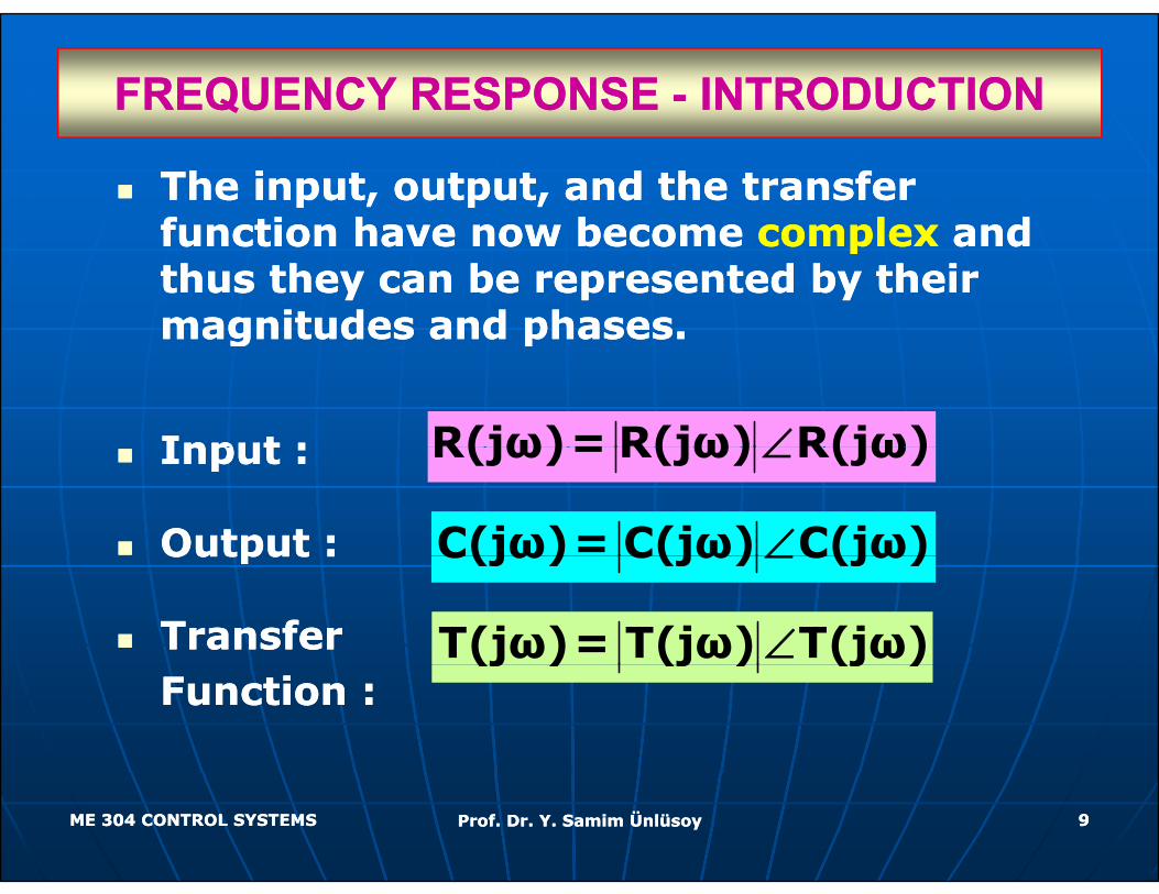
The input, output, and the transfer The input, output, and the transfer function have now become function have now become complexcomplex and and function have now become function have now become complexcomplex and and thus they can be represented by their thus they can be represented by their magnitudes and phases.magnitudes and phases.magnitudes and phases.magnitudes and phases.
Input :Input : R(jω)= R(jω) R(jω)∠Input :Input :
Output :Output : C(jω)= C(jω) C(jω)∠
R(jω)= R(jω) R(jω)∠
Output :Output :
TransferTransfer
C(jω) C(jω) C(jω)∠
T(jω)= T(jω) Τ(jω)∠Function :Function :
(j ) (j ) (j )
ME 304 CONTROL SYSTEMSME 304 CONTROL SYSTEMS Prof. Dr. Y. Samim ÜnlüsoyProf. Dr. Y. Samim Ünlüsoy 99
FREQUENCY RESPONSE FREQUENCY RESPONSE -- INTRODUCTIONINTRODUCTION
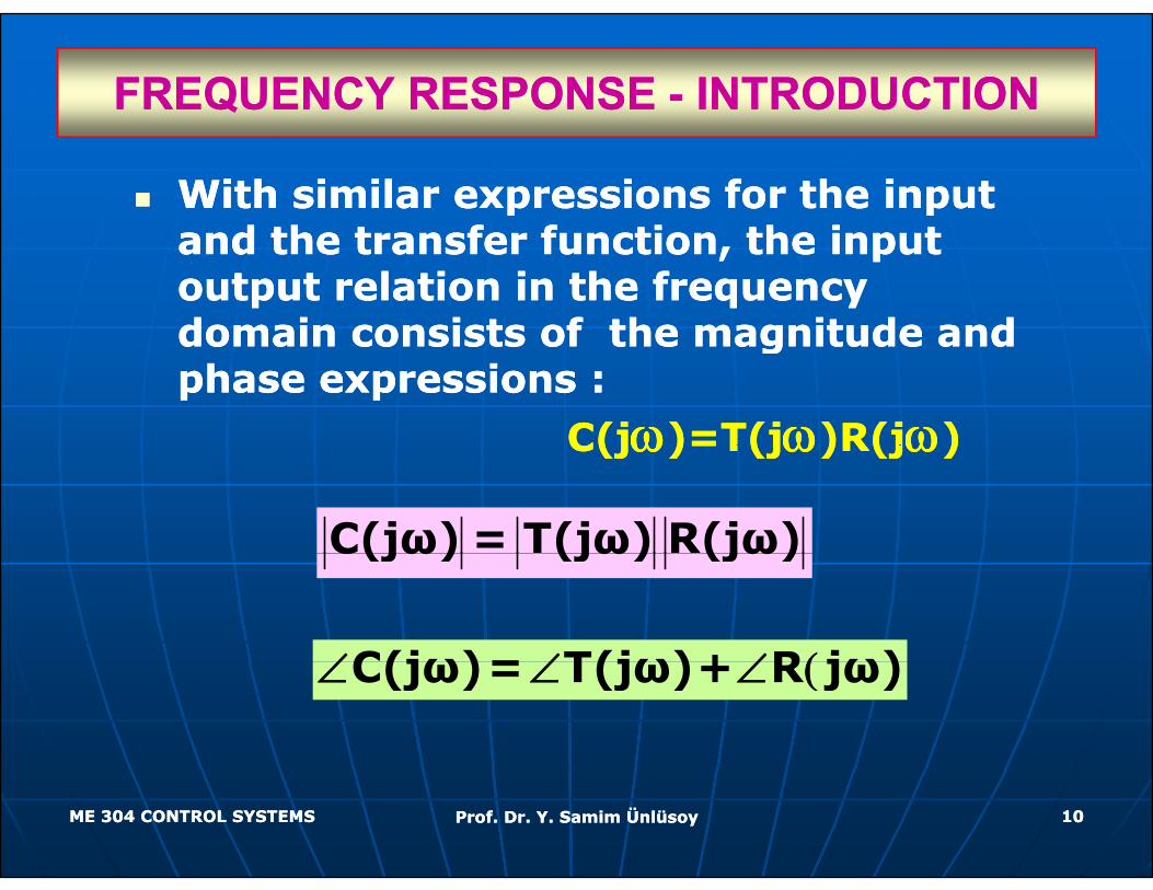
With similar expressions for the input With similar expressions for the input d th t f f ti th i t d th t f f ti th i t and the transfer function, the input and the transfer function, the input
output relation in the frequency output relation in the frequency domain consists of the magnitude and domain consists of the magnitude and domain consists of the magnitude and domain consists of the magnitude and phase expressions :phase expressions :
C(jC(jωω)=T(j)=T(jωω)R(j)R(jωω))C(jC(jωω)=T(j)=T(jωω)R(j)R(jωω))
C(jω) = T(jω) R(jω)C(jω) (jω) (jω)
C(jω)= T(jω)+ R jω)∠ ∠ ∠ (C(jω)= T(jω)+ R jω)∠ ∠ ∠ (
ME 304 CONTROL SYSTEMSME 304 CONTROL SYSTEMS Prof. Dr. Y. Samim ÜnlüsoyProf. Dr. Y. Samim Ünlüsoy 1010
FREQUENCY RESPONSE FREQUENCY RESPONSE -- INTRODUCTIONINTRODUCTION
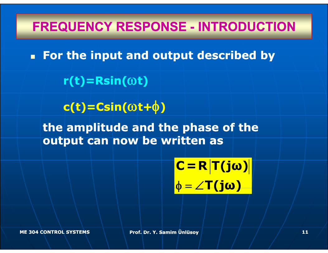
For the input and output described byFor the input and output described by
r(t)=Rsin(r(t)=Rsin(ωωt)t)
c(t)=Csin(c(t)=Csin(ωωt+t+φφ))
the amplitude and the phase of the the amplitude and the phase of the the amplitude and the phase of the the amplitude and the phase of the output can now be written asoutput can now be written as
C=R T(jω)
T(jω)φ = ∠T(jω)φ ∠
ME 304 CONTROL SYSTEMSME 304 CONTROL SYSTEMS Prof. Dr. Y. Samim ÜnlüsoyProf. Dr. Y. Samim Ünlüsoy 1111
FREQUENCY RESPONSEFREQUENCY RESPONSE
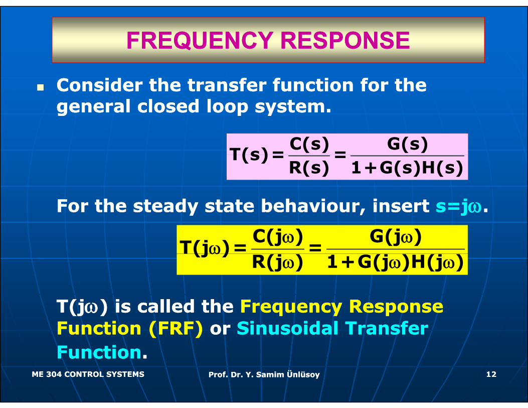
Consider the transfer function for the Consider the transfer function for the general closed loop systemgeneral closed loop systemgeneral closed loop system.general closed loop system.
C(s) G(s)T(s)= =
For the steady state behaviour insert For the steady state behaviour insert s=js=jωω
T(s)= =R(s) 1+G(s)H(s)
For the steady state behaviour, insert For the steady state behaviour, insert s=js=jωω..
C(j ) G(j )T(j )= =
ω ωω
T(jT(jωω) is called the ) is called the Frequency Response Frequency Response
T(j )R(j ) 1+G(j )H(j )
ωω ω ω
T(jT(jωω) is called the ) is called the Frequency Response Frequency Response Function (FRF) Function (FRF) or or Sinusoidal Transfer Sinusoidal Transfer FunctionFunction
ME 304 CONTROL SYSTEMSME 304 CONTROL SYSTEMS Prof. Dr. Y. Samim ÜnlüsoyProf. Dr. Y. Samim Ünlüsoy 1212
FunctionFunction..
FREQUENCY RESPONSEFREQUENCY RESPONSEFREQUENCY RESPONSEFREQUENCY RESPONSE
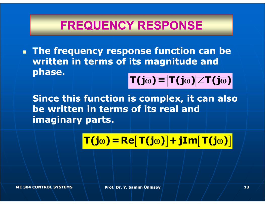
The frequency response function can be The frequency response function can be The frequency response function can be The frequency response function can be written in terms of its magnitude and written in terms of its magnitude and phase.phase.
T(j ) T(j ) T(j )∠
Since this function is complex, it can also Since this function is complex, it can also
T(j )= T(j ) T(j )ω ω ∠ ω
p ,p ,be written in terms of its real and be written in terms of its real and imaginary parts. imaginary parts.
[ ] [ ]T(j )=Re T(j ) + jIm T(j )ω ω ω
ME 304 CONTROL SYSTEMSME 304 CONTROL SYSTEMS Prof. Dr. Y. Samim ÜnlüsoyProf. Dr. Y. Samim Ünlüsoy 1313
FREQUENCY RESPONSEFREQUENCY RESPONSE
R b th t f l b b R b th t f l b b
FREQUENCY RESPONSEFREQUENCY RESPONSE
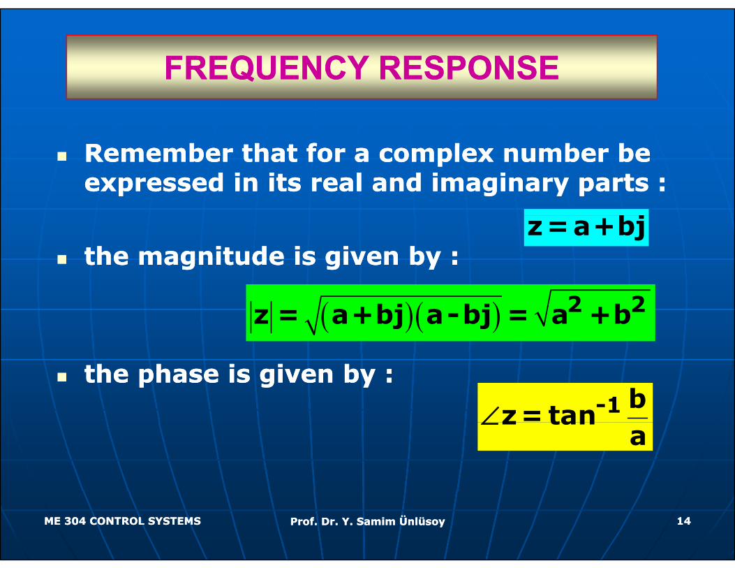
Remember that for a complex number be Remember that for a complex number be expressed in its real and imaginary parts :expressed in its real and imaginary parts :
the magnitude is given by : the magnitude is given by : z=a+bj
( )( ) 2 2z = a+bj a-bj = a +b
the phase is given by :the phase is given by :-1 b
z= tan∠z tana
∠
ME 304 CONTROL SYSTEMSME 304 CONTROL SYSTEMS Prof. Dr. Y. Samim ÜnlüsoyProf. Dr. Y. Samim Ünlüsoy 1414
FREQUENCY RESPONSEFREQUENCY RESPONSEQQ
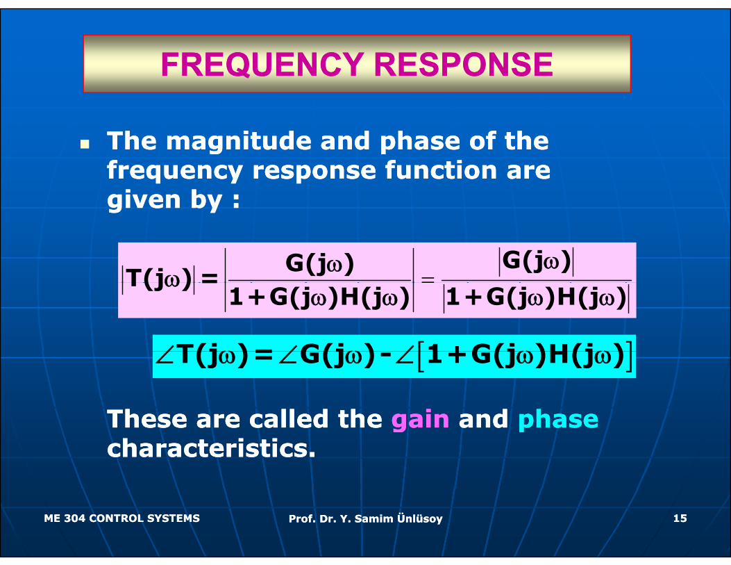
The magnitude and phase of the The magnitude and phase of the The magnitude and phase of the The magnitude and phase of the frequency response function are frequency response function are given by :given by :
=G(j )G(j )
T(j ) =ωω
ω =T(j ) =1+G(j )H(j ) 1+G(j )H(j )
ωω ω ω ω
[ ]T(j )= G(j ) 1+G(j )H(j )∠ ω ∠ ω ∠ ω ω
These are called the These are called the gain gain and and phase phase
[ ]T(j )= G(j )- 1+G(j )H(j )∠ ω ∠ ω ∠ ω ω
These are called the These are called the gain gain and and phase phase characteristics.characteristics.
ME 304 CONTROL SYSTEMSME 304 CONTROL SYSTEMS Prof. Dr. Y. Samim ÜnlüsoyProf. Dr. Y. Samim Ünlüsoy 1515
FREQUENCY RESPONSE FREQUENCY RESPONSE –– Example 1aExample 1app
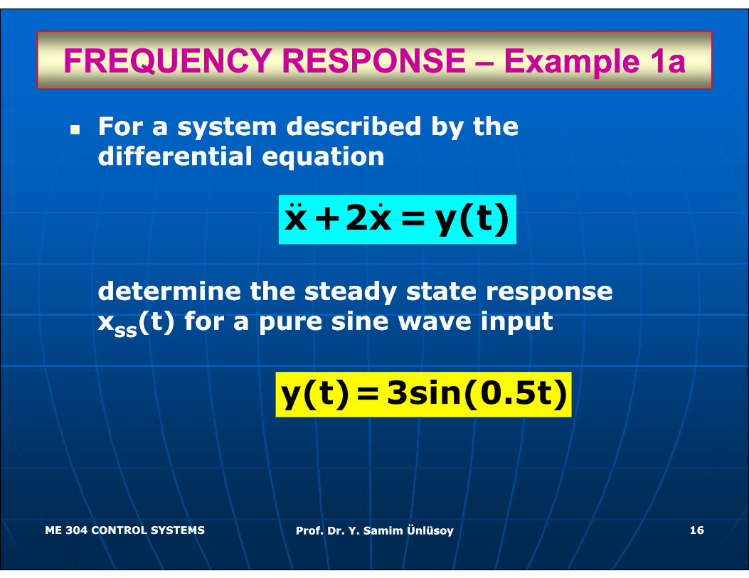
For a system described by the For a system described by the diff ti l tidiff ti l tidifferential equationdifferential equation
x+2x = y(t)
determine the steady state response determine the steady state response
x+2x = y(t)
determine the steady state response determine the steady state response xxssss(t) for a pure sine wave input(t) for a pure sine wave input
y(t)=3sin(0.5t)
ME 304 CONTROL SYSTEMSME 304 CONTROL SYSTEMS Prof. Dr. Y. Samim ÜnlüsoyProf. Dr. Y. Samim Ünlüsoy 1616
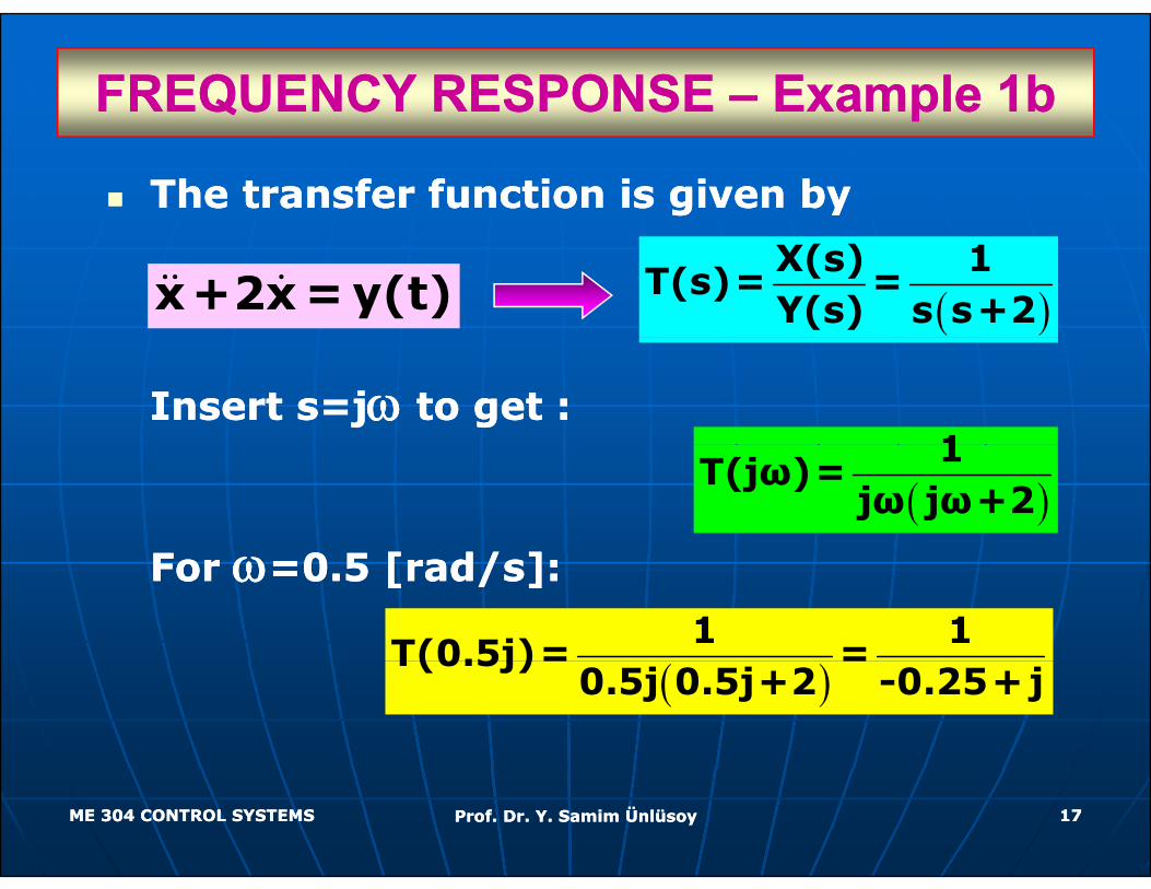
FREQUENCY RESPONSE FREQUENCY RESPONSE –– Example 1bExample 1bpp
The transfer function is given byThe transfer function is given by
x+2x = y(t) ( )X(s) 1
T(s)= =Y(s) s s+2
Insert s=jInsert s=jωω to get :to get :1
0 [ d/ ]0 [ d/ ]
( )1
T(jω)=jω jω+2
For For ωω=0.5 [rad/s]:=0.5 [rad/s]:
1 1T(0.5j)= =
( )T(0.5j)= =
0.5j 0.5j+2 -0.25+j
ME 304 CONTROL SYSTEMSME 304 CONTROL SYSTEMS Prof. Dr. Y. Samim ÜnlüsoyProf. Dr. Y. Samim Ünlüsoy 1717
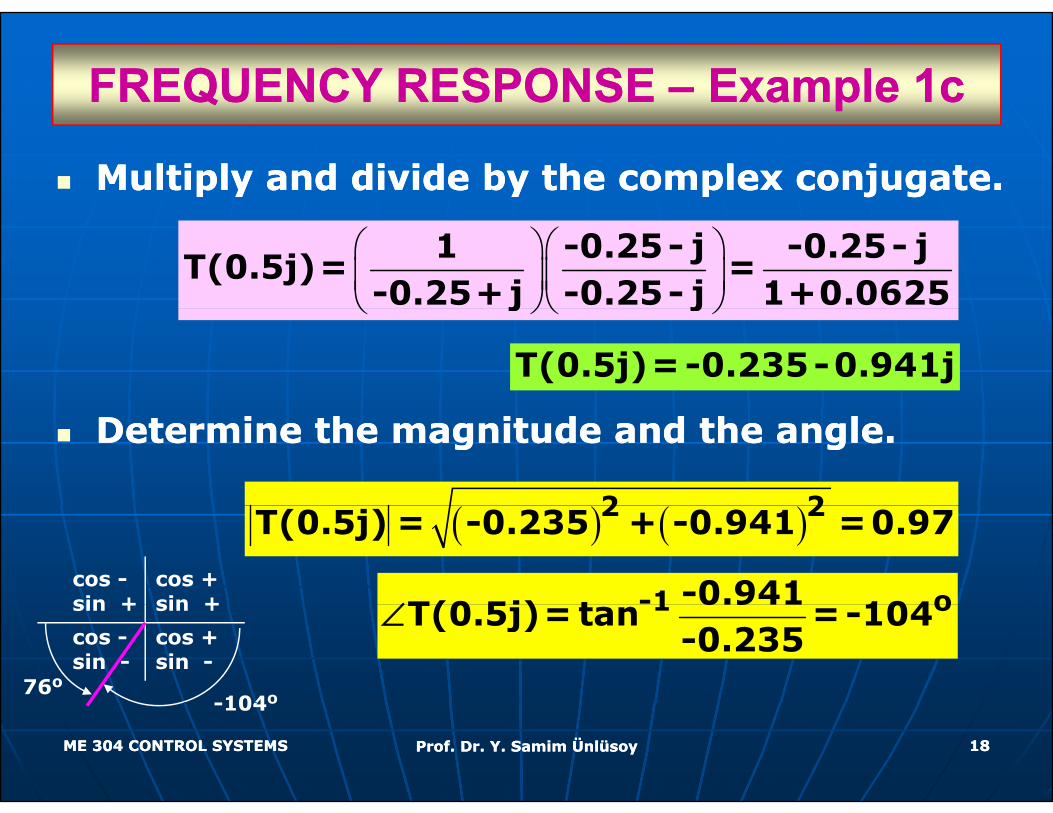
FREQUENCY RESPONSE FREQUENCY RESPONSE –– Example 1cExample 1cpp
Multiply and divide by the complex conjugate.Multiply and divide by the complex conjugate.
⎛ ⎞⎛ ⎞⎜ ⎟⎜ ⎟⎝ ⎠⎝ ⎠
1 -0.25- j -0.25- jT(0.5j)= =
-0.25+j -0.25- j 1+0.0625⎝ ⎠⎝ ⎠j j
T(0.5j)=-0.235-0.941j
Determine the magnitude and the angle. Determine the magnitude and the angle.
2 2( ) ( )2 2T(0.5j) = -0.235 + -0.941 =0.97
-1 o-0.941T(0 5j) t 104∠
cos +sin +
cos -sin + 1 o0.941
T(0.5j)= tan =-104-0.235
∠sin +sin +
cos -sin -
cos +sin -
76o-104o
ME 304 CONTROL SYSTEMSME 304 CONTROL SYSTEMS Prof. Dr. Y. Samim ÜnlüsoyProf. Dr. Y. Samim Ünlüsoy 1818
-104o
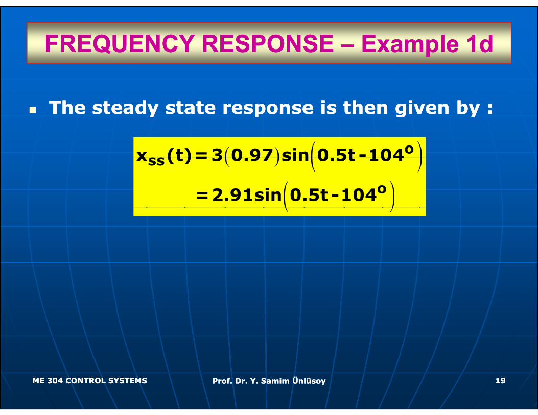
FREQUENCY RESPONSE FREQUENCY RESPONSE –– Example 1dExample 1dpp
The steady state response is then given by :The steady state response is then given by :The steady state response is then given by :The steady state response is then given by :
( ) ( )ox (t)=3 0 97 sin 0 5t -104( ) ( )( )
ss
o
x (t)=3 0.97 sin 0.5t 104
=2.91sin 0.5t -104( )
ME 304 CONTROL SYSTEMSME 304 CONTROL SYSTEMS Prof. Dr. Y. Samim ÜnlüsoyProf. Dr. Y. Samim Ünlüsoy 1919
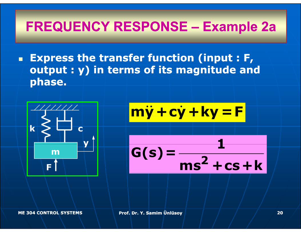
FREQUENCY RESPONSE FREQUENCY RESPONSE –– Example 2aExample 2aQQ pp
Express the transfer function (input : F, Express the transfer function (input : F, Express the transfer function (input : F, Express the transfer function (input : F, output : y) in terms of its magnitude and output : y) in terms of its magnitude and phase.phase.
my+cy+ky =Fmy+cy+ky F
1k c
y
21
G(s)=ms +cs+k
m
F
y
ME 304 CONTROL SYSTEMSME 304 CONTROL SYSTEMS Prof. Dr. Y. Samim ÜnlüsoyProf. Dr. Y. Samim Ünlüsoy 2020
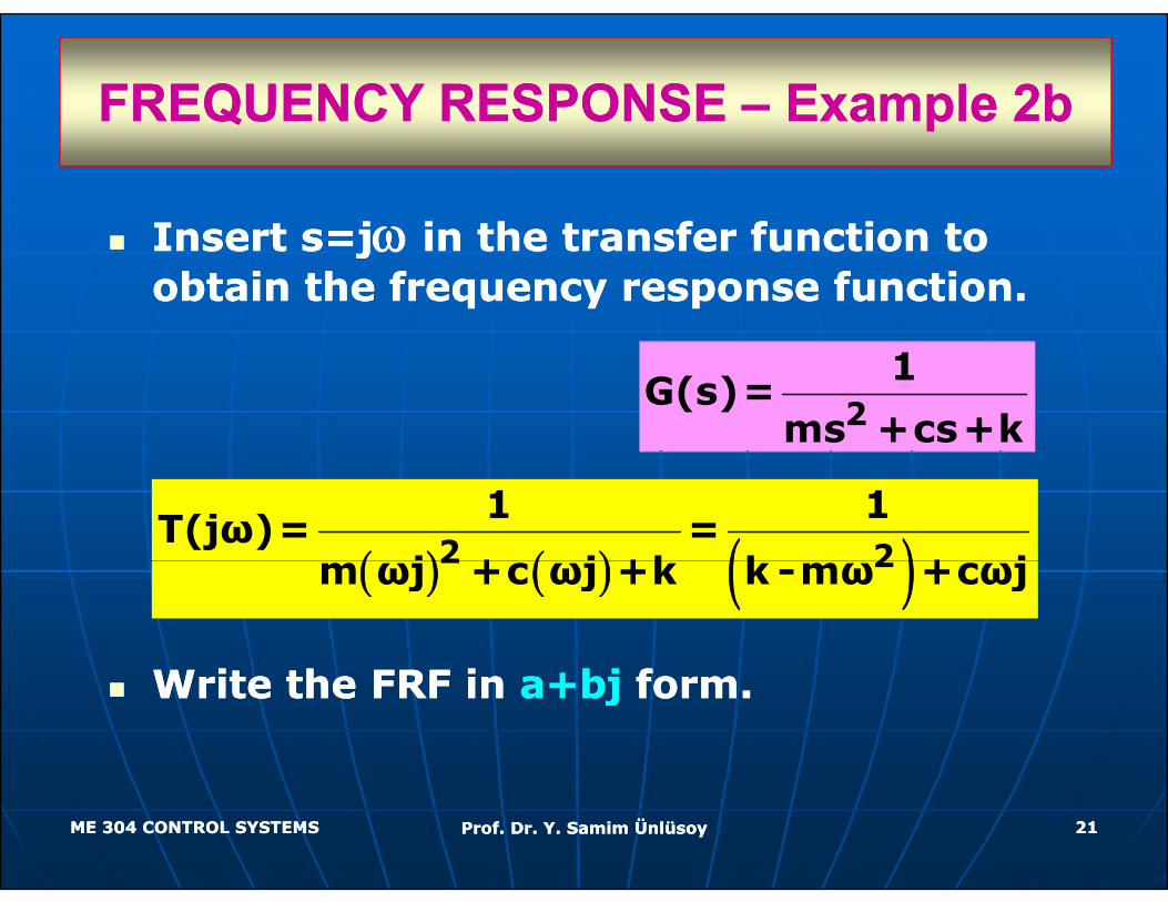
FREQUENCY RESPONSE FREQUENCY RESPONSE –– Example 2bExample 2bQQ pp
Insert s=jInsert s=jωω in the transfer function to in the transfer function to Insert s=jInsert s=jωω in the transfer function to in the transfer function to obtain the frequency response function.obtain the frequency response function.
21
G(s)=ms +cs+k
( ) ( ) ( )2 2
1 1T(jω)= =
j + j +k k + j
W i h FRF i W i h FRF i bjbj ff
( ) ( ) ( )2 2m ωj +c ωj +k k -mω +cωj
Write the FRF in Write the FRF in a+bja+bj form.form.
ME 304 CONTROL SYSTEMSME 304 CONTROL SYSTEMS Prof. Dr. Y. Samim ÜnlüsoyProf. Dr. Y. Samim Ünlüsoy 2121
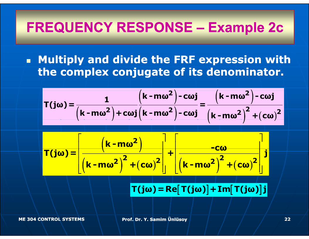
FREQUENCY RESPONSE FREQUENCY RESPONSE –– Example 2cExample 2cQQ pp
Multiply and divide the FRF expression with Multiply and divide the FRF expression with Multiply and divide the FRF expression with Multiply and divide the FRF expression with the complex conjugate of its denominator.the complex conjugate of its denominator.
( ) ( )2 2
( )( )( )
( )( ) ( )
2 2
22 2 22
k -mω -cωj k -mω -cωj1T(jω)= =
k -mω +cωj k -mω -cωj k -mω + cω( ) ( ) ( ) ( )
( )2k -mω -cω⎡ ⎤ ⎡ ⎤⎢ ⎥ ⎢ ⎥( )( ) ( ) ( ) ( )
2 22 22 2
cωT(jω)= + j
k -mω + cω k -mω + cω
⎢ ⎥ ⎢ ⎥⎢ ⎥ ⎢ ⎥⎢ ⎥ ⎢ ⎥⎢ ⎥ ⎢ ⎥⎣ ⎦ ⎣ ⎦
[ ] [ ]T(jω)=Re T(jω) +Im T(jω) j
ME 304 CONTROL SYSTEMSME 304 CONTROL SYSTEMS Prof. Dr. Y. Samim ÜnlüsoyProf. Dr. Y. Samim Ünlüsoy 2222
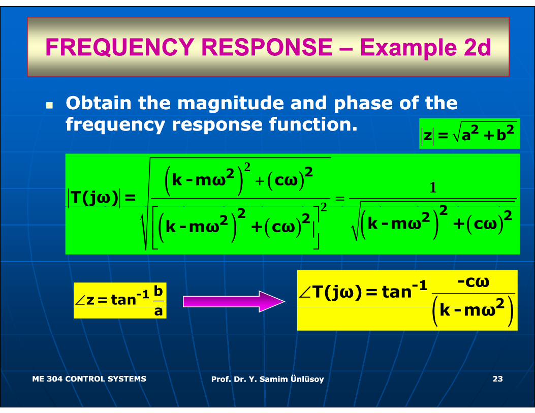
FREQUENCY RESPONSE FREQUENCY RESPONSE –– Example 2dExample 2dQQ pp
Obtain the magnitude and phase of the Obtain the magnitude and phase of the Obtain the magnitude and phase of the Obtain the magnitude and phase of the frequency response function.frequency response function. 2 2z = a +b
( ) ( )2
21
22
2
k -mω cωT(jω) =
+=
⎡ ⎤( ) ( ) ( ) ( )2 22 2222 k -mω + cωk -mω + cω
⎡ ⎤⎢ ⎥⎣ ⎦
( )-1
2
-cωT(jω)= tan
k mω∠-1 b
z= tan∠ ( )2k -mωa
ME 304 CONTROL SYSTEMSME 304 CONTROL SYSTEMS Prof. Dr. Y. Samim ÜnlüsoyProf. Dr. Y. Samim Ünlüsoy 2323
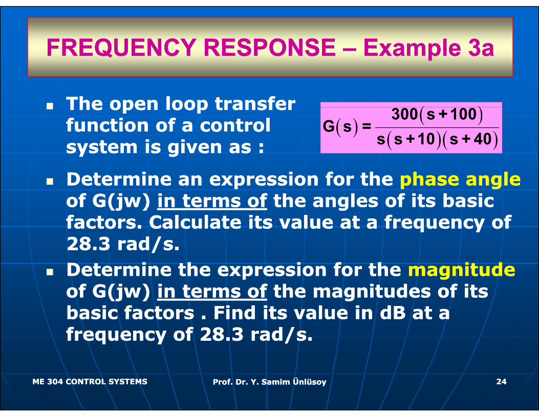
FREQUENCY RESPONSE FREQUENCY RESPONSE –– Example 3aExample 3aQQ pp
The open loop transferThe open loop transfer ( )The open loop transferThe open loop transferfunction of a control function of a control system is given as :system is given as :
( ) ( )( )( )300 s +100
G s =s s +10 s + 40
Determine an expression for the Determine an expression for the phase anglephase angleof G(jw) of G(jw) in terms ofin terms of the angles of its basic the angles of its basic (j )(j ) ggfactorsfactors.. Calculate its valueCalculate its value at a frequency of at a frequency of 28.3 rad/s.28.3 rad/s.Determine the expression for the Determine the expression for the magnitude magnitude of G(jw) of G(jw) in terms ofin terms of the magnitudes of its the magnitudes of its basic factors basic factors Find its al e in dB at a Find its al e in dB at a basic factors basic factors .. Find its value in dB at a Find its value in dB at a frequency of 28.3 rad/s.frequency of 28.3 rad/s.
ME 304 CONTROL SYSTEMSME 304 CONTROL SYSTEMS Prof. Dr. Y. Samim ÜnlüsoyProf. Dr. Y. Samim Ünlüsoy 2424
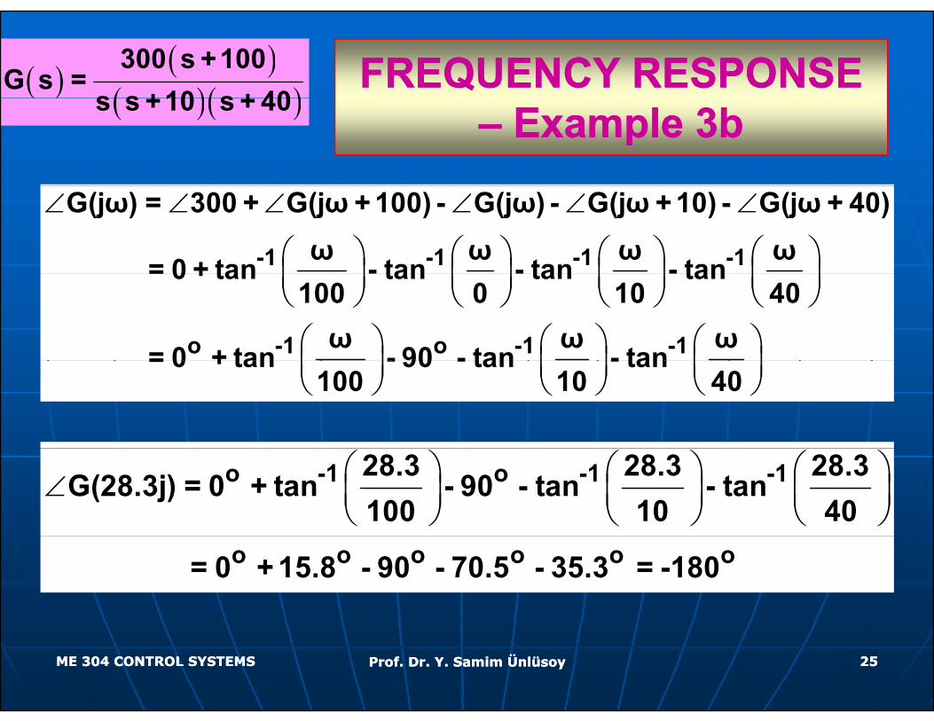
FREQUENCY RESPONSE FREQUENCY RESPONSE ( ) ( )( )( )300 s +100
G s =s s +10 s + 40 –– Example 3bExample 3b
( ) ( )( )s s +10 s + 40
∠ ∠ ∠ ∠ ∠ ∠
⎛ ⎞ ⎛ ⎞ ⎛ ⎞ ⎛ ⎞⎜ ⎟ ⎜ ⎟ ⎜ ⎟ ⎜ ⎟
-1 -1 -1 -1
G(jω) = 300 + G(jω + 100) - G(jω) - G(jω + 10) - G(jω + 40)ω ω ω ω= 0 + tan - tan - tan - tan⎜ ⎟ ⎜ ⎟ ⎜ ⎟ ⎜ ⎟
⎝ ⎠ ⎝ ⎠ ⎝ ⎠ ⎝ ⎠⎛ ⎞ ⎛ ⎞ ⎛ ⎞⎜ ⎟ ⎜ ⎟ ⎜ ⎟
o -1 o -1 -1
= 0 + tan - tan - tan - tan100 0 10 40ω ω ω= 0 + tan - 90 - tan - tan⎜ ⎟ ⎜ ⎟ ⎜ ⎟
⎝ ⎠ ⎝ ⎠ ⎝ ⎠= 0 + tan - 90 - tan - tan
100 10 40
∠ ⎛ ⎞ ⎛ ⎞ ⎛ ⎞⎜ ⎟ ⎜ ⎟ ⎜ ⎟⎝ ⎠ ⎝ ⎠ ⎝ ⎠
o -1 o -1 -128.3 28.3 28.3G(28.3j) = 0 + tan - 90 - tan - tan100 10 40
o o o o o o= 0 + 15.8 - 90 - 70.5 - 35.3 = -180
ME 304 CONTROL SYSTEMSME 304 CONTROL SYSTEMS Prof. Dr. Y. Samim ÜnlüsoyProf. Dr. Y. Samim Ünlüsoy 2525

FREQUENCY RESPONSE FREQUENCY RESPONSE ( ) ( )( )( )300 s +100
G s =s s +10 s + 40 –– Example 3cExample 3c
( ) ( )( )s s +10 s + 40
300 j 100( )
300 jω + 100G jω =
jω jω + 10 jω + 40
2 2
2 2 2 2
300 ω + 100=
2 2 2 2ω ω + 10 ω + 40
2 2300 28 3 + 100( )2 2 2 2
300 28.3 + 100G 28.3j =
28.3 28.3 + 10 28.3 + 40
( )( )( )( )( )
300 103.9= = 0.749
28.3 30.0 49.0
ME 304 CONTROL SYSTEMSME 304 CONTROL SYSTEMS Prof. Dr. Y. Samim ÜnlüsoyProf. Dr. Y. Samim Ünlüsoy 2626
FREQUENCY RESPONSEFREQUENCY RESPONSEFREQUENCY RESPONSEFREQUENCY RESPONSE
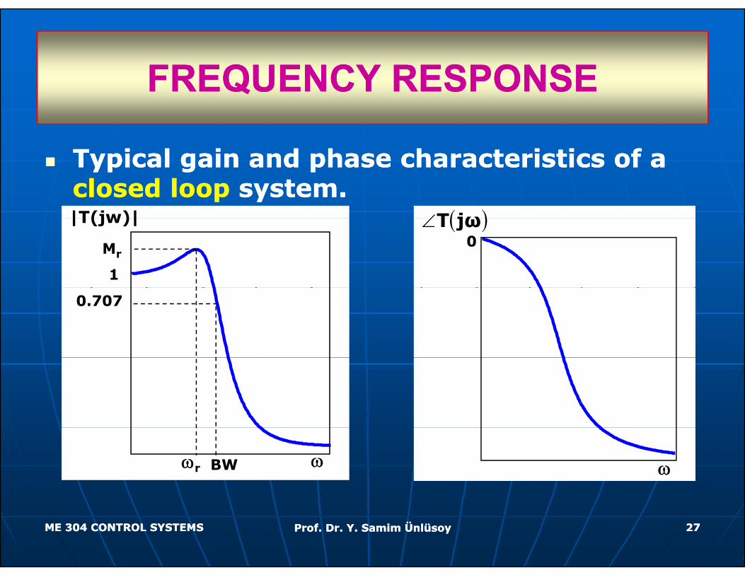
Typical gain and phase characteristics of a Typical gain and phase characteristics of a closed loopclosed loop system.system.|T(jw)| ( )jωT∠
1
Mr
|T(jw)|0
( )jωT∠
0.707
ωωr BW ω
ME 304 CONTROL SYSTEMSME 304 CONTROL SYSTEMS Prof. Dr. Y. Samim ÜnlüsoyProf. Dr. Y. Samim Ünlüsoy 2727
FREQUENCY DOMAIN SPECIFICATIONSFREQUENCY DOMAIN SPECIFICATIONSQQ
Similar to transient response Similar to transient response Similar to transient response Similar to transient response specifications in time domain, specifications in time domain, frequency response specifications are frequency response specifications are frequency response specifications are frequency response specifications are defined.defined.
-- Resonant peak, MResonant peak, Mrr,,
-- Resonant frequency, Resonant frequency, ωωrr,,Resonant frequency, Resonant frequency, ωωrr,,
-- Bandwidth, BW,Bandwidth, BW,ffff-- Cutoff Rate.Cutoff Rate.
ME 304 CONTROL SYSTEMSME 304 CONTROL SYSTEMS Prof. Dr. Y. Samim ÜnlüsoyProf. Dr. Y. Samim Ünlüsoy 2828
FREQUENCY DOMAIN SPECIFICATIONSFREQUENCY DOMAIN SPECIFICATIONSQQ
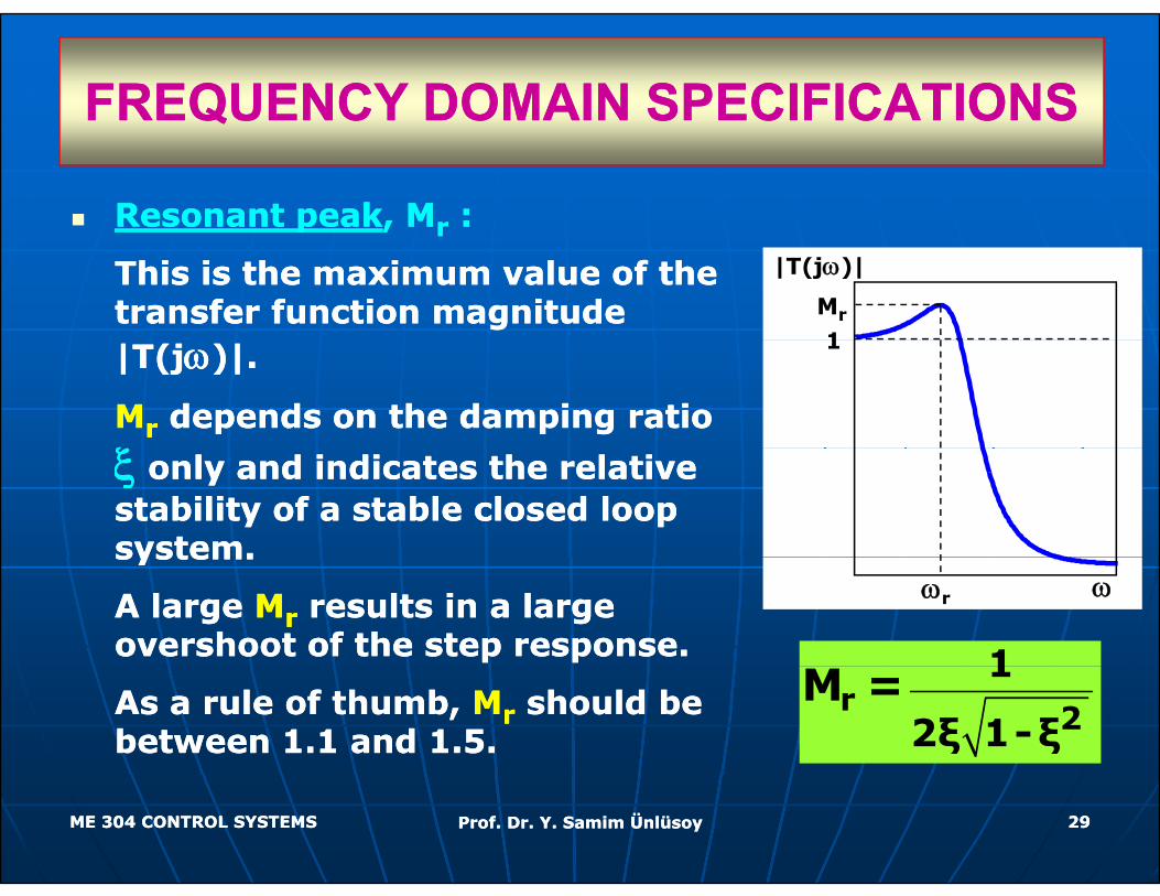
Resonant peakResonant peak, M, Mrr ::pp ,, rr
This is the maximum value of the This is the maximum value of the transfer function magnitude transfer function magnitude
1
Mr
|T(jω)|
|T(j|T(jωω)|. )|.
MMrr depends on the damping ratio depends on the damping ratio
ξξ
1
ξξ only and indicates the relative only and indicates the relative stability of a stable closed loop stability of a stable closed loop system.system.system.system.
A large A large MMrr results in a large results in a large overshoot of the step response.overshoot of the step response. 1
ωωr
As a rule of thumb, As a rule of thumb, MMrr should be should be between 1.1 and 1.5.between 1.1 and 1.5.
r 2
1
2ξ 1-ξM =
ME 304 CONTROL SYSTEMSME 304 CONTROL SYSTEMS Prof. Dr. Y. Samim ÜnlüsoyProf. Dr. Y. Samim Ünlüsoy 2929
FREQUENCY DOMAIN SPECIFICATIONSFREQUENCY DOMAIN SPECIFICATIONSQQ
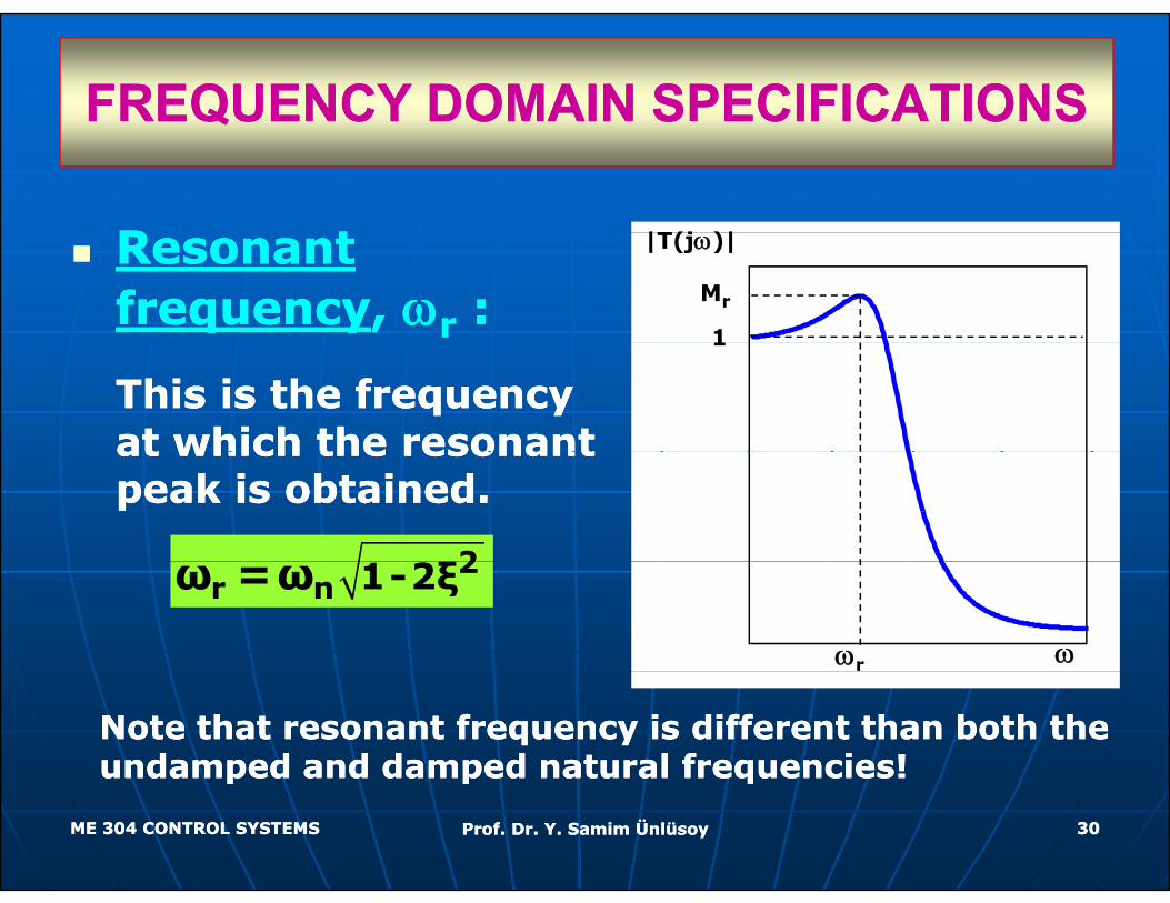
R t R t |T(j )|Resonant Resonant frequencyfrequency, , ωωrr ::
1
Mr
|T(jω)|
This is the frequency This is the frequency at which the resonant at which the resonant
1
at which the resonant at which the resonant peak is obtained.peak is obtained.
22r n 1-2ξω =ω
ωωr
Note that resonant frequency is different than both the Note that resonant frequency is different than both the undamped and damped natural frequencies!undamped and damped natural frequencies!
ME 304 CONTROL SYSTEMSME 304 CONTROL SYSTEMS Prof. Dr. Y. Samim ÜnlüsoyProf. Dr. Y. Samim Ünlüsoy 3030
p p qp p q
FREQUENCY DOMAIN SPECIFICATIONSFREQUENCY DOMAIN SPECIFICATIONS
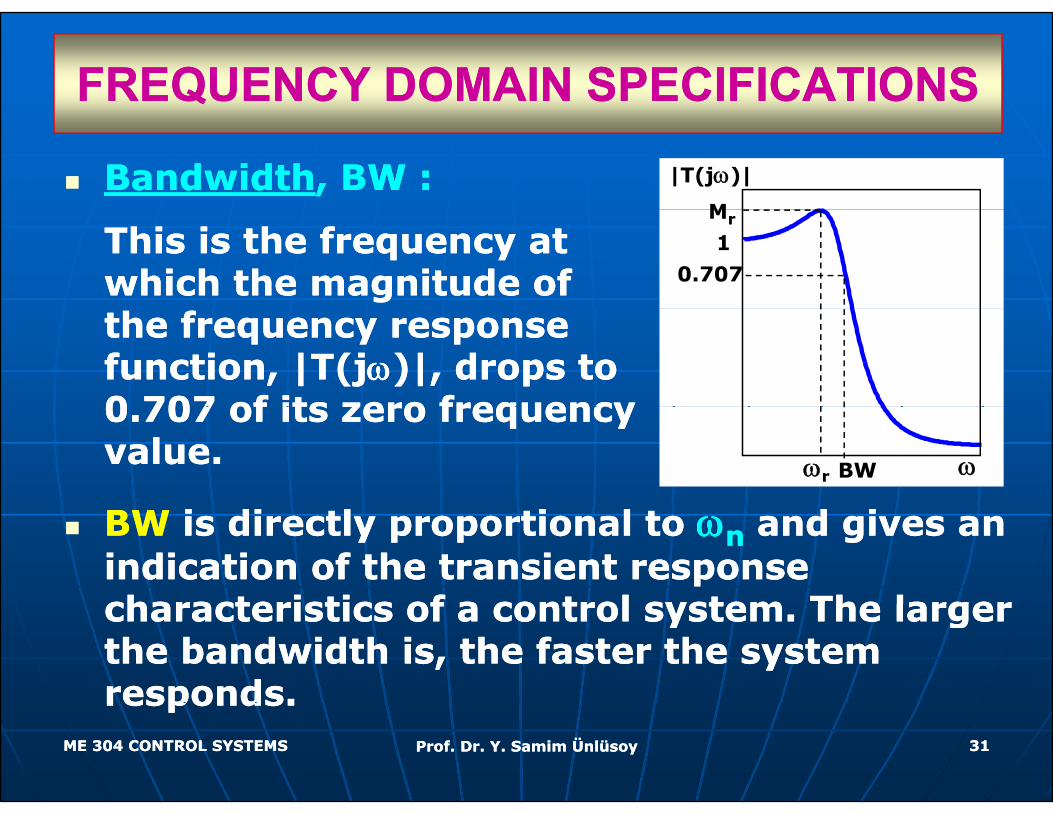
BandwidthBandwidth, BW :, BW :M
|T(jω)|
This is the frequency at This is the frequency at which the magnitude of which the magnitude of
1
0.707
Mr
the frequency response the frequency response function, |T(jfunction, |T(jωω)|, drops to )|, drops to 0 707 of its zero frequency 0 707 of its zero frequency 0.707 of its zero frequency 0.707 of its zero frequency value. value. ωωr BW
BWBW is directly proportional to is directly proportional to ωωnn and gives an and gives an indication of the transient response indication of the transient response characteristics of a control system The larger characteristics of a control system The larger characteristics of a control system. The larger characteristics of a control system. The larger the bandwidth is, the faster the system the bandwidth is, the faster the system responds.responds.
ME 304 CONTROL SYSTEMSME 304 CONTROL SYSTEMS Prof. Dr. Y. Samim ÜnlüsoyProf. Dr. Y. Samim Ünlüsoy 3131
responds.responds.
FREQUENCY DOMAIN SPECIFICATIONSFREQUENCY DOMAIN SPECIFICATIONSQU C O S C C O SQU C O S C C O S
|T(jω)|
1
0 707
Mr
|T(jω)|
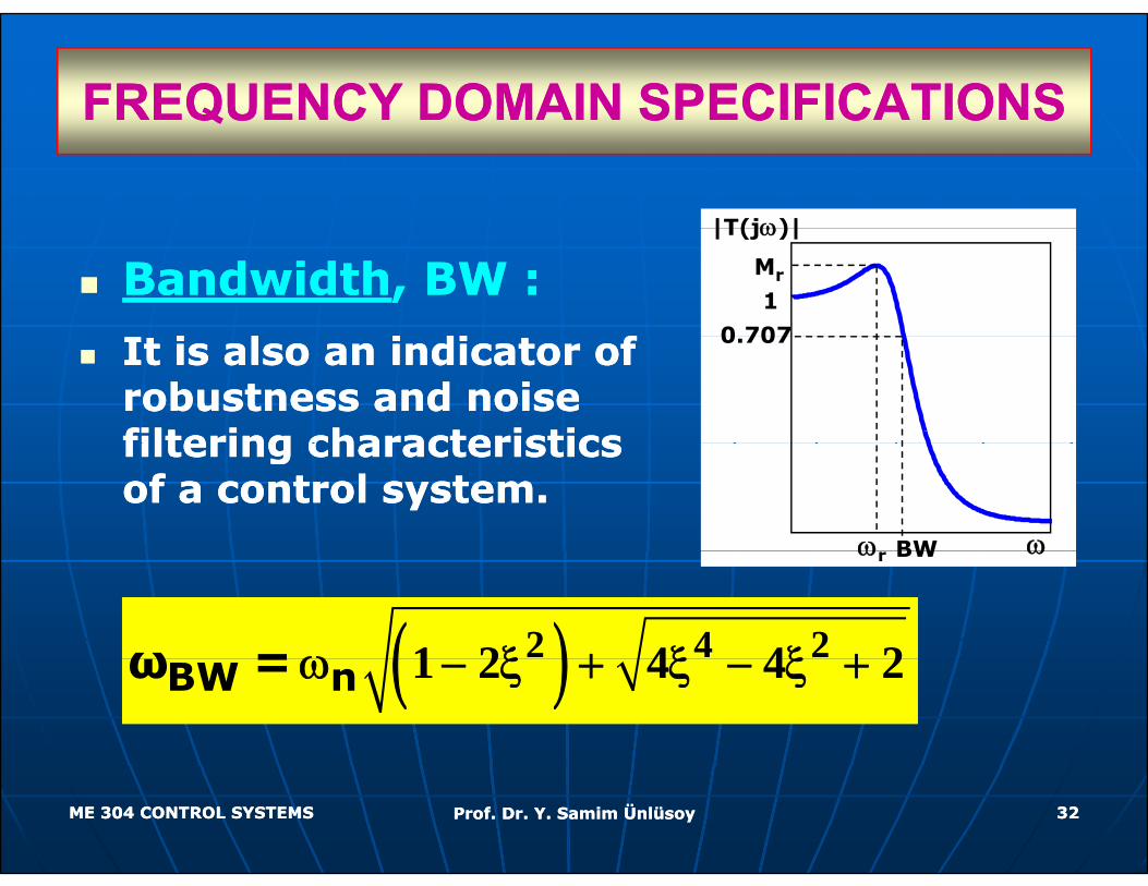
BandwidthBandwidth, BW :, BW :
ff 0.707It is also an indicator of It is also an indicator of robustness and noise robustness and noise filtering characteristics filtering characteristics
ωω BW
filtering characteristics filtering characteristics of a control system.of a control system.
ωωr BW
( )2 4 21 2 4 4 2ω = ω ξ + ξ ξ +( )1 2 4 4 2BW nω = ω − ξ + ξ − ξ +
ME 304 CONTROL SYSTEMSME 304 CONTROL SYSTEMS Prof. Dr. Y. Samim ÜnlüsoyProf. Dr. Y. Samim Ünlüsoy 3232
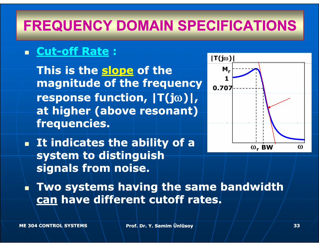
FREQUENCY DOMAIN SPECIFICATIONSFREQUENCY DOMAIN SPECIFICATIONSCutCut--off Rateoff Rate ::
|T(jω)|
This is the This is the slopeslope of the of the magnitude of the frequency magnitude of the frequency
f i | (jf i | (j )|)|
1
0.707
Mr
response function, |T(jresponse function, |T(jωω)|, )|, at higher (above resonant) at higher (above resonant) frequencies frequencies frequencies. frequencies.
It indicates the ability of a It indicates the ability of a t t di ti i h t t di ti i h
ωωr BW
system to distinguish system to distinguish signals from noise.signals from noise.
T h i h b d id h T h i h b d id h Two systems having the same bandwidth Two systems having the same bandwidth cancan have different cutoff rates.have different cutoff rates.
ME 304 CONTROL SYSTEMSME 304 CONTROL SYSTEMS Prof. Dr. Y. Samim ÜnlüsoyProf. Dr. Y. Samim Ünlüsoy 3333
BODE PLOT BODE PLOT Dorf & Bishop Ch 8Dorf & Bishop Ch 8 Ogata Ch 8Ogata Ch 8Dorf & Bishop Ch. 8,Dorf & Bishop Ch. 8, Ogata Ch. 8Ogata Ch. 8
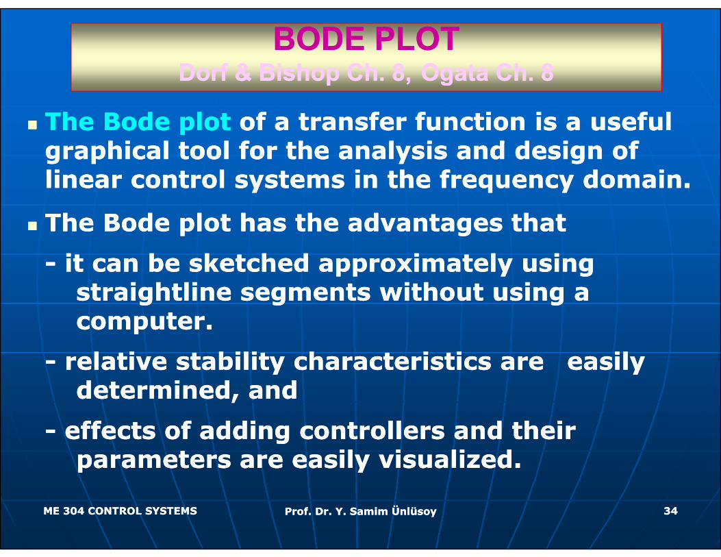
The Bode plot The Bode plot of a transfer function is a useful of a transfer function is a useful hi l t l f th l i d d i f hi l t l f th l i d d i f graphical tool for the analysis and design of graphical tool for the analysis and design of
linear control systems in the frequency domain.linear control systems in the frequency domain.
The Bode plot has the advantages thatThe Bode plot has the advantages that
-- it can be sketched approximately using it can be sketched approximately using straightline segments without using a straightline segments without using a computer.computer.
-- relative stability characteristics are relative stability characteristics are easily easily determined, anddetermined, and
-- effects of adding controllers and their effects of adding controllers and their parameters are easily visualized.parameters are easily visualized.
ME 304 CONTROL SYSTEMSME 304 CONTROL SYSTEMS Prof. Dr. Y. Samim ÜnlüsoyProf. Dr. Y. Samim Ünlüsoy 3434
BODE PLOTBODE PLOT
ME 304 CONTROL SYSTEMSME 304 CONTROL SYSTEMS Prof. Dr. Y. Samim ÜnlüsoyProf. Dr. Y. Samim Ünlüsoy 3535
BODE PLOTBODE PLOTNise Section 10 2Nise Section 10 2Nise Section 10.2Nise Section 10.2
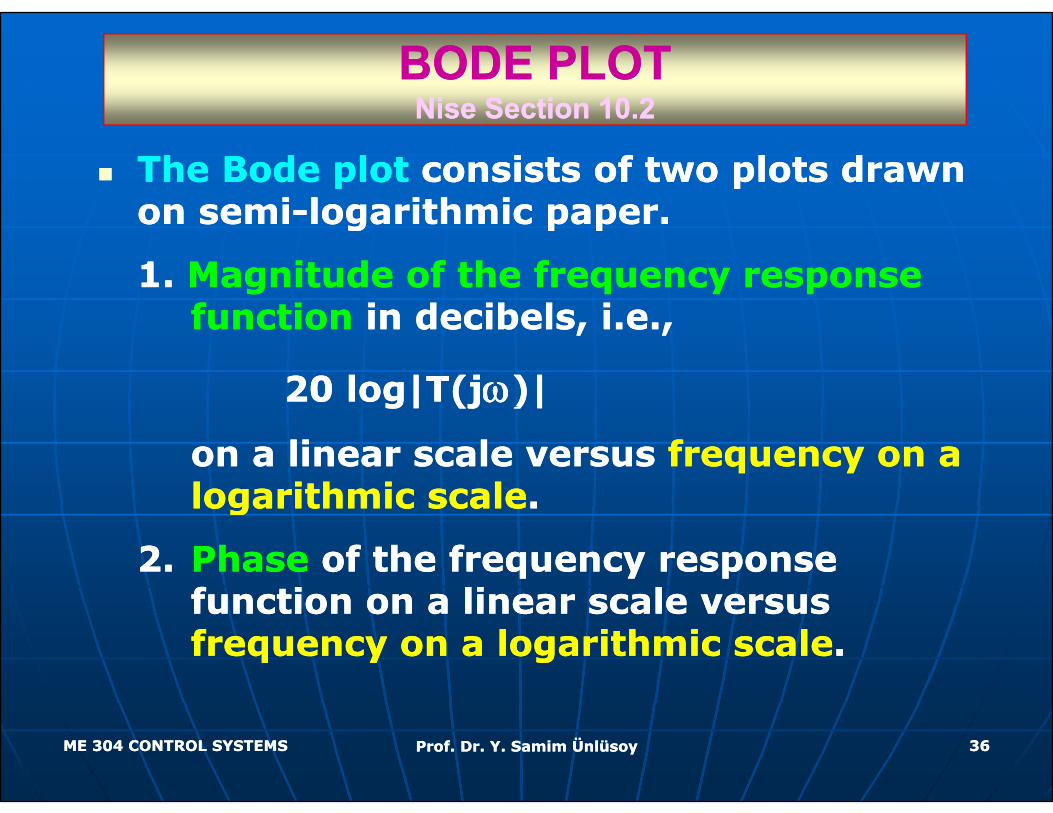
The Bode plot The Bode plot consists of two plots drawn consists of two plots drawn on semion semi logarithmic paperlogarithmic paperon semion semi--logarithmic paper.logarithmic paper.
1. 1. Magnitude of the frequency response Magnitude of the frequency response f tif ti i d ib l ii d ib l ifunctionfunction in decibels, i.e.,in decibels, i.e.,
20 log|T(j20 log|T(jωω)|)|g| (jg| (j )|)|
on a linear scale versus on a linear scale versus frequency on a frequency on a logarithmic scalelogarithmic scale..logarithmic scalelogarithmic scale..
2.2. PhasePhase of the frequency response of the frequency response function on a linear scale versus function on a linear scale versus function on a linear scale versus function on a linear scale versus frequency on a logarithmic scalefrequency on a logarithmic scale..
ME 304 CONTROL SYSTEMSME 304 CONTROL SYSTEMS Prof. Dr. Y. Samim ÜnlüsoyProf. Dr. Y. Samim Ünlüsoy 3636
BODE PLOTBODE PLOT
ME 304 CONTROL SYSTEMSME 304 CONTROL SYSTEMS Prof. Dr. Y. Samim ÜnlüsoyProf. Dr. Y. Samim Ünlüsoy 3737
BODE PLOTBODE PLOT
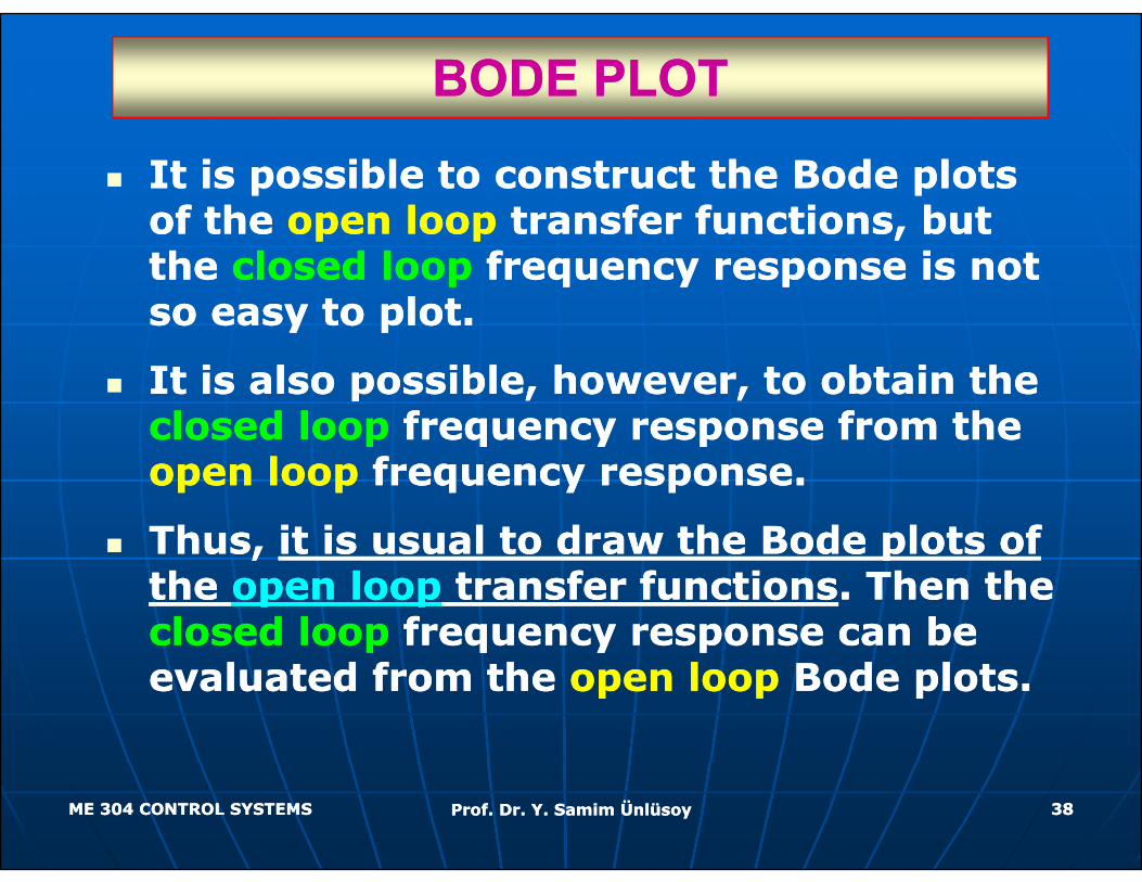
It is possible to construct the Bode plots It is possible to construct the Bode plots of the of the open loopopen loop transfer functions, but transfer functions, but of the of the open loopopen loop transfer functions, but transfer functions, but the the closed loopclosed loop frequency response is not frequency response is not so easy to plot.so easy to plot.
It is also possible, however, to obtain the It is also possible, however, to obtain the closed loopclosed loop frequency response from the frequency response from the pp q y pq y popen loopopen loop frequency response.frequency response.
Thus, Thus, it is usual to draw the Bode plots of it is usual to draw the Bode plots of Thus, Thus, it is usual to draw the Bode plots of it is usual to draw the Bode plots of the the open loopopen loop transfer functionstransfer functions. Then the . Then the closed loopclosed loop frequency response can be frequency response can be evaluated from the evaluated from the open loopopen loop Bode plots.Bode plots.
ME 304 CONTROL SYSTEMSME 304 CONTROL SYSTEMS Prof. Dr. Y. Samim ÜnlüsoyProf. Dr. Y. Samim Ünlüsoy 3838
BODE PLOTBODE PLOT
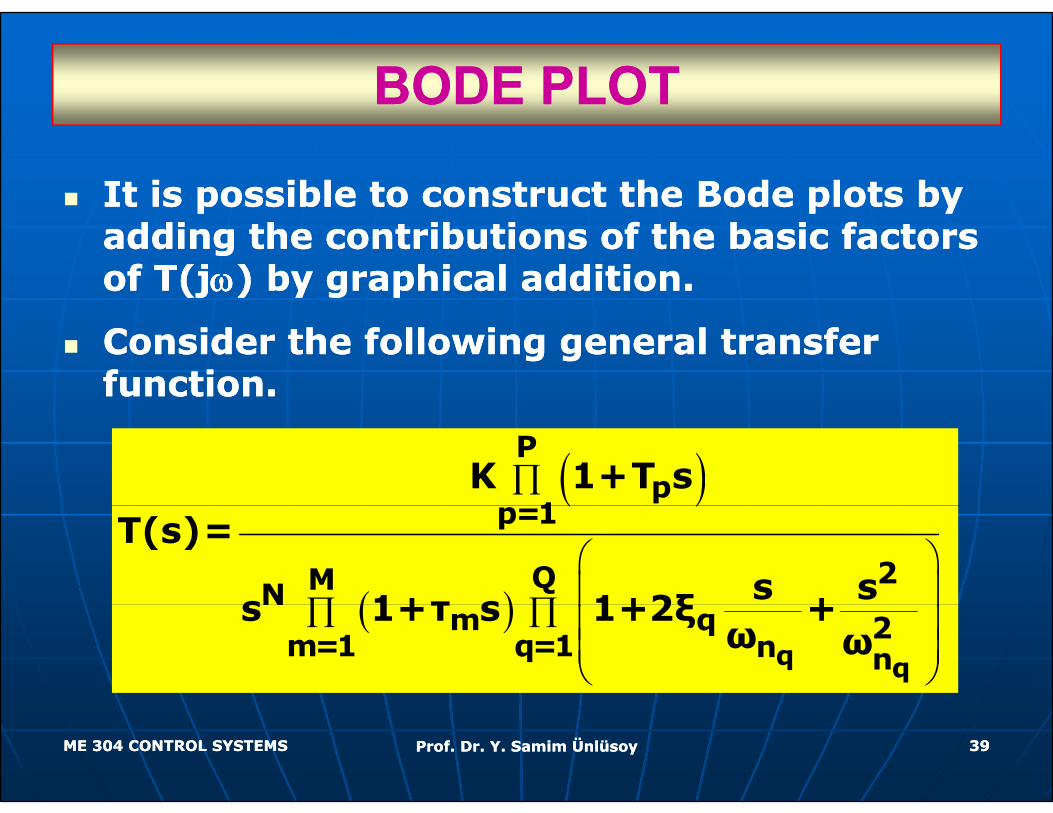
It is possible to construct the Bode plots by It is possible to construct the Bode plots by p p yp p yadding the contributions of the basic factors adding the contributions of the basic factors of T(jof T(jωω) by graphical addition.) by graphical addition.
Consider the following general transfer Consider the following general transfer function.function.
( )∏P
p1
K 1+T s( )
( )⎛ ⎞⎜ ⎟∏ ∏
p=1
2QMN
T(s)=
s ss 1+τ s 1+2ξ +( ) ⎜ ⎟∏ ∏ ⎜ ⎟
⎜ ⎟⎝ ⎠q q
Nm q 2
m=1 q=1 n n
s 1+τ s 1+2ξ +ω ω
ME 304 CONTROL SYSTEMSME 304 CONTROL SYSTEMS Prof. Dr. Y. Samim ÜnlüsoyProf. Dr. Y. Samim Ünlüsoy 3939
BODE PLOTBODE PLOT( )
( )
∏
⎛ ⎞⎜ ⎟
∏ ∏
Pp
p=1
2QMN
K 1+T s
T(s)=
s ss 1+τ s 1+2ξ +( ) ⎜ ⎟
∏ ∏ ⎜ ⎟⎜ ⎟⎝ ⎠q q
Nm q 2m=1 q=1 n n
s 1+τ s 1+2ξ +ω ω
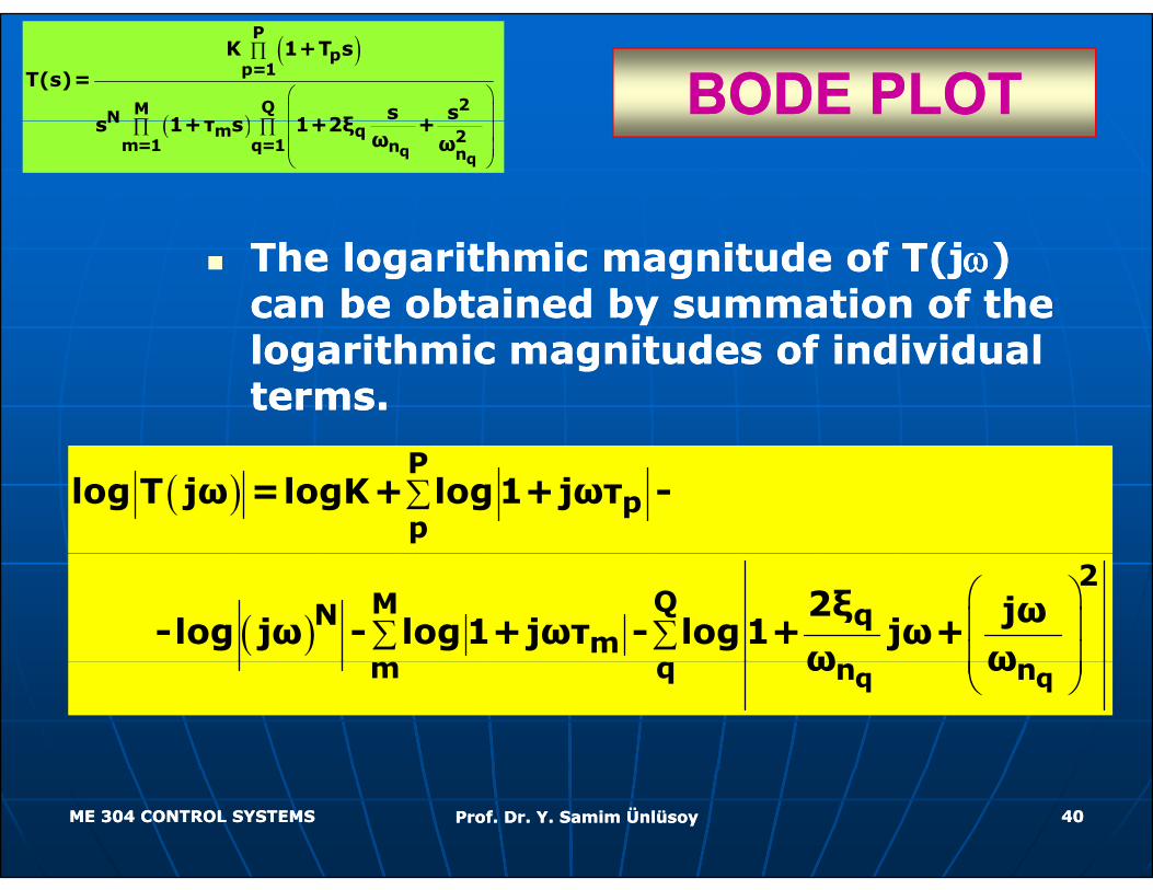
The logarithmic magnitude of T(jThe logarithmic magnitude of T(jωω) ) can be obtained by summation of the can be obtained by summation of the l ith i it d f i di id l l ith i it d f i di id l logarithmic magnitudes of individual logarithmic magnitudes of individual terms.terms.
( ) ∑P
pp
log T jω =logK+ log1+jωτ -
( )⎛ ⎞⎜ ⎟∑ ∑⎜ ⎟⎝ ⎠
2QMN q
m2ξ jω
-log jω - log1+jωτ - log1+ jω+ω ω⎜ ⎟
⎝ ⎠q qm q n nω ω
ME 304 CONTROL SYSTEMSME 304 CONTROL SYSTEMS Prof. Dr. Y. Samim ÜnlüsoyProf. Dr. Y. Samim Ünlüsoy 4040
BODE PLOTBODE PLOT( )
( )
∏
⎛ ⎞⎜ ⎟
∏ ∏ ⎜ ⎟
Pp
p=1
2QMNm q 2
K 1+T s
T(s)=
s ss 1+τ s 1+2ξ +( )∏ ∏ ⎜ ⎟
⎜ ⎟⎝ ⎠q q
m q 2m=1 q=1 n n
s 1+τ s 1+2ξ +ω ω
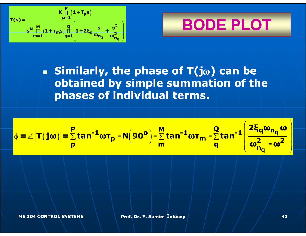
Similarly, the phase of T(jSimilarly, the phase of T(jωω) can be ) can be obtained by simple summation of the obtained by simple summation of the phases of individual terms.phases of individual terms.
( ) ( )⎛ ⎞⎜ ⎟
∑ ∑ ∑ ⎜ ⎟⎜ ⎟⎝ ⎠
qQP M q n-1 o -1 -1p m 2 2p m q n
2ξ ω ω= T jω = tan ωτ -N 90 - tan ωτ - tan
ω -ωφ ∠
⎜ ⎟⎝ ⎠q
p q n
ME 304 CONTROL SYSTEMSME 304 CONTROL SYSTEMS Prof. Dr. Y. Samim ÜnlüsoyProf. Dr. Y. Samim Ünlüsoy 4141
BODE PLOTBODE PLOT
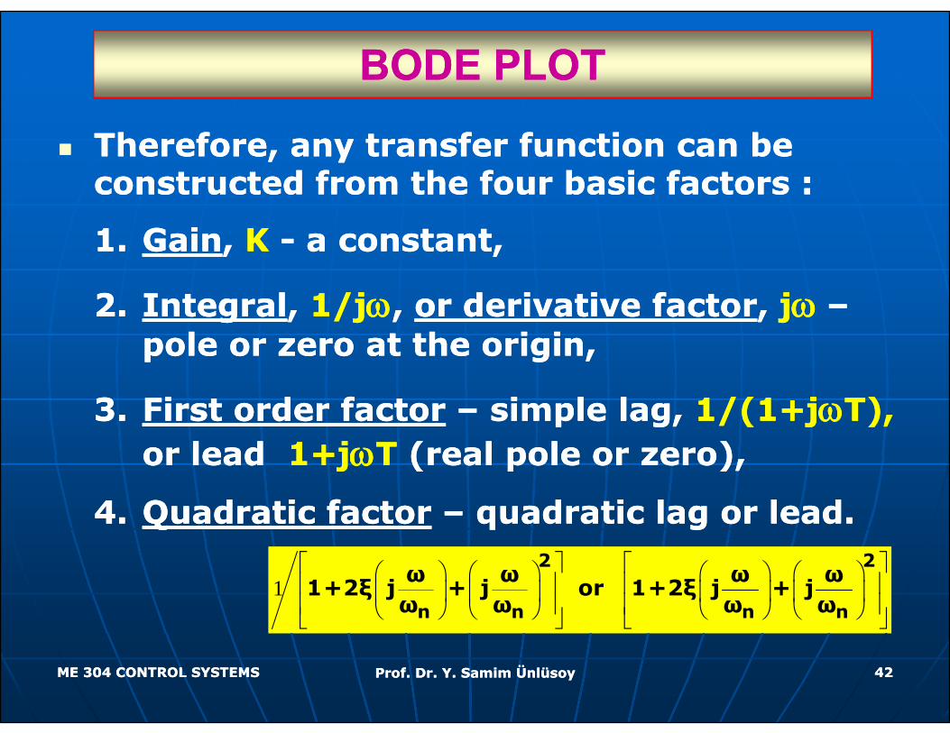
Therefore, any transfer function can be Therefore, any transfer function can be constructed from the four basic factors :constructed from the four basic factors :constructed from the four basic factors :constructed from the four basic factors :
1.1. GainGain, , KK -- a constant,a constant,
2.2. IntegralIntegral, , 1/j1/jωω, , or derivative factoror derivative factor, , jjω ω ––pole or zero at the origin,pole or zero at the origin,
3.3. First order factorFirst order factor –– simple lag, simple lag, 1/(1+j1/(1+jωωT),T),or lead or lead 1+j1+jωωT T (real pole or zero)(real pole or zero)or lead or lead 1+j1+jωωT T (real pole or zero),(real pole or zero),
4.4. Quadratic factorQuadratic factor –– quadratic lag or lead.quadratic lag or lead.
1⎡ ⎤ ⎡ ⎤⎛ ⎞ ⎛ ⎞ ⎛ ⎞ ⎛ ⎞⎢ ⎥ ⎢ ⎥⎜ ⎟ ⎜ ⎟ ⎜ ⎟ ⎜ ⎟⎢ ⎥ ⎢ ⎥⎝ ⎠ ⎝ ⎠ ⎝ ⎠ ⎝ ⎠⎣ ⎦ ⎣ ⎦
2 2
n n n n
ω ω ω ω1+2ξ j + j or 1+2ξ j + j
ω ω ω ω
ME 304 CONTROL SYSTEMSME 304 CONTROL SYSTEMS Prof. Dr. Y. Samim ÜnlüsoyProf. Dr. Y. Samim Ünlüsoy 4242
BODE PLOTBODE PLOT
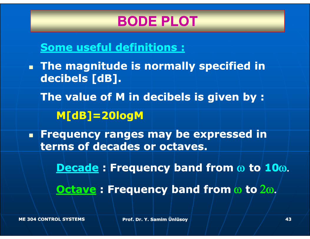
Some useful definitions :Some useful definitions :
The magnitude is normally specified in The magnitude is normally specified in decibels [dB].decibels [dB].
The value of M in decibels is given by :The value of M in decibels is given by :
M[dB]=20logMM[dB]=20logM[ ] g[ ] g
Frequency ranges may be expressed in Frequency ranges may be expressed in terms of decades or octaves.terms of decades or octaves.terms of decades or octaves.terms of decades or octaves.
DecadeDecade : Frequency band from : Frequency band from ωω to to 1010ωω..
OctaveOctave : Frequency band from: Frequency band from ωω toto 2ω2ω..
ME 304 CONTROL SYSTEMSME 304 CONTROL SYSTEMS Prof. Dr. Y. Samim ÜnlüsoyProf. Dr. Y. Samim Ünlüsoy 4343
BODE PLOTBODE PLOT
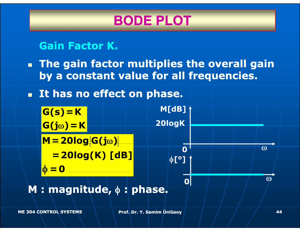
Gain Factor K.Gain Factor K.
The gain factor multiplies the overall gain The gain factor multiplies the overall gain by a constant value for all frequencies.by a constant value for all frequencies.
It has no effect on phase.It has no effect on phase.
G(s)=K M[dB]( )G(j )=Kω
M=20log G(j )ω
20logK
M 20log G(j )
=20log(K) [dB]
=0
ω
φ
ω0φ[o]
M : magnitude, M : magnitude, φφ : phase.: phase.
0φω0
ME 304 CONTROL SYSTEMSME 304 CONTROL SYSTEMS Prof. Dr. Y. Samim ÜnlüsoyProf. Dr. Y. Samim Ünlüsoy 4444
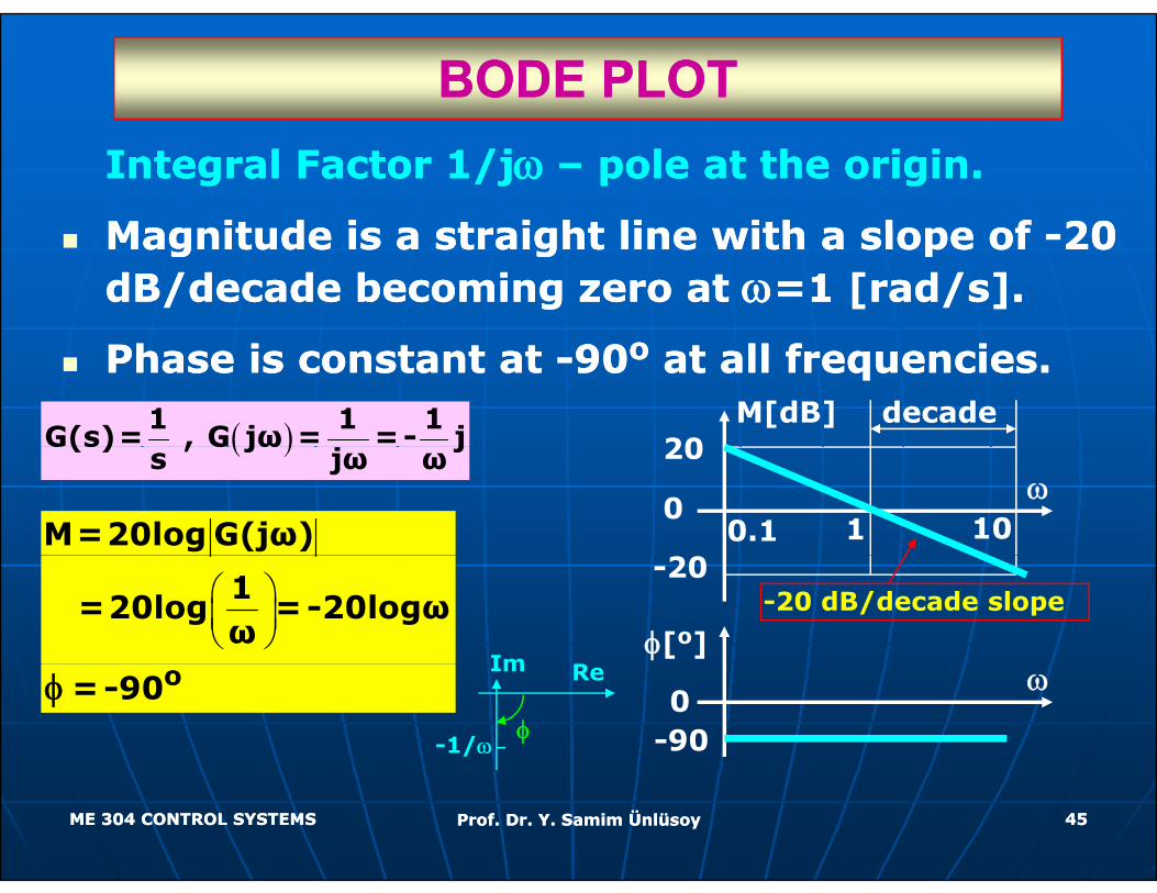
BODE PLOTBODE PLOTIntegral Factor 1/jIntegral Factor 1/jω ω –– pole at the origin.pole at the origin.
Magnitude is a straight line with a slope of Magnitude is a straight line with a slope of 20 20 Magnitude is a straight line with a slope of Magnitude is a straight line with a slope of --20 20 dB/decade becoming zero at dB/decade becoming zero at ωω=1 [rad/s].=1 [rad/s].
Phase is constant at Phase is constant at --9090oo at all frequencies.at all frequencies.
( )1 1 1G(s)= , G jω = =- j
M[dB]20
decade( )G(s) , G jω j
s jω ω
M=20log G(jω)
20ω
00.1 1 10
⎛ ⎞⎜ ⎟⎝ ⎠
1=20log =-20logω
ω
-20
φ[o]-20 dB/decade slope
Imo=-90 φ 0-90
ωReIm
-1/ωφ
ME 304 CONTROL SYSTEMSME 304 CONTROL SYSTEMS Prof. Dr. Y. Samim ÜnlüsoyProf. Dr. Y. Samim Ünlüsoy 4545
BODE PLOTBODE PLOT ReIm-1/ω2
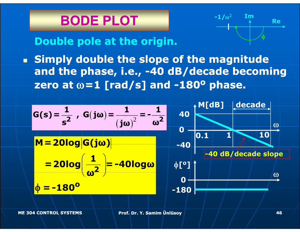
Double pole at the origin.Double pole at the origin.
Simply double the slope of the magnitude Simply double the slope of the magnitude
φ
Simply double the slope of the magnitude Simply double the slope of the magnitude and the phase, i.e., and the phase, i.e., --40 dB/decade becoming 40 dB/decade becoming zero at zero at ωω=1 [rad/s] and =1 [rad/s] and --180180oo phase.phase.zero at zero at ωω 1 [rad/s] and 1 [rad/s] and 180180 phase.phase.
( )1 1 1G(s)= , G jω = =-
M[dB]40
decade( )
( )22 2G(s)= , G jω = =
s ωjω
M=20log G(jω)
ω40
0
400.1 1 10
⎛ ⎞⎜ ⎟⎝ ⎠2
M=20log G(jω)
1=20log =-40logω
ω
-40
φ[o]-40 dB/decade slope
⎝ ⎠oω
=-180 φω
0-180
ME 304 CONTROL SYSTEMSME 304 CONTROL SYSTEMS Prof. Dr. Y. Samim ÜnlüsoyProf. Dr. Y. Samim Ünlüsoy 4646
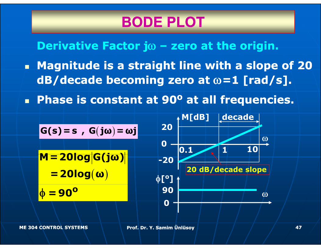
BODE PLOTBODE PLOTDerivative Factor jDerivative Factor jω ω –– zero at the origin.zero at the origin.
Magnitude is a straight line with a slope of 20 Magnitude is a straight line with a slope of 20 Magnitude is a straight line with a slope of 20 Magnitude is a straight line with a slope of 20 dB/decade becoming zero at dB/decade becoming zero at ωω=1 [rad/s].=1 [rad/s].
Phase is constant at 90Phase is constant at 90oo at all frequencies.at all frequencies.
M[dB]20
decade
( )G(s)=s , G jω =ωj
M 20l G(j )
20ω
00.1 1 10
( )M=20log G(jω)
=20log ω-20
φ[o]20 dB/decade slope
o=90 φ0
90 ω
ME 304 CONTROL SYSTEMSME 304 CONTROL SYSTEMS Prof. Dr. Y. Samim ÜnlüsoyProf. Dr. Y. Samim Ünlüsoy 4747
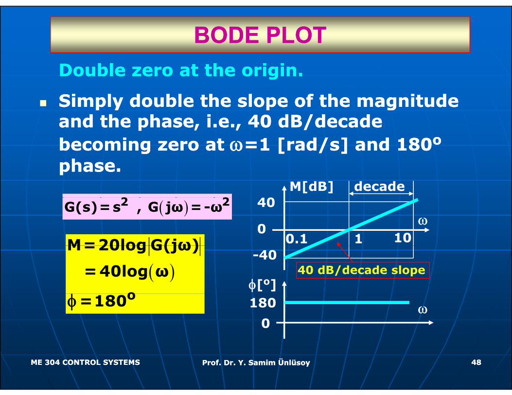
BODE PLOTBODE PLOTDouble zero at the origin.Double zero at the origin.
Simply double the slope of the magnitude Simply double the slope of the magnitude Simply double the slope of the magnitude Simply double the slope of the magnitude and the phase, i.e., 40 dB/decade and the phase, i.e., 40 dB/decade becoming zero at becoming zero at ωω=1 [rad/s] and 180=1 [rad/s] and 180oobecoming zero at becoming zero at ωω 1 [rad/s] and 1801 [rad/s] and 180phase.phase.
2 2M[dB]
0decade
( )2 2G(s)=s , G jω =-ω
M=20log G(jω)
40ω
00.1 1 10
( )o
M=20log G(jω)
=40log ω-40
φ[o]40 dB/decade slope
o=180φ0
180 ω
ME 304 CONTROL SYSTEMSME 304 CONTROL SYSTEMS Prof. Dr. Y. Samim ÜnlüsoyProf. Dr. Y. Samim Ünlüsoy 4848
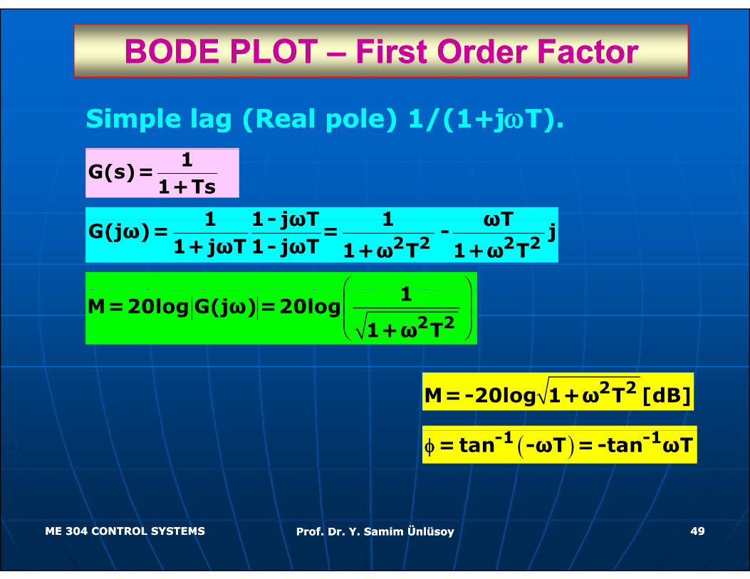
BODE PLOT BODE PLOT –– First Order FactorFirst Order Factor
Simple lag (Real pole) 1/(1+jSimple lag (Real pole) 1/(1+jωωT).T).
1G(s)=
1+Ts
1 1- jωT 1 ωT
⎛ ⎞1
2 2 2 21 1- jωT 1 ωT
G(jω)= = - j1+jωT 1- jωT 1+ω T 1+ω T
⎛ ⎞⎜ ⎟⎜ ⎟⎝ ⎠2 2
1M=20log G(jω)=20log
1+ω T
2 2M=-20log 1+ω T [dB]
( )-1 -1= tan -ωT =-tan ωTφ
ME 304 CONTROL SYSTEMSME 304 CONTROL SYSTEMS Prof. Dr. Y. Samim ÜnlüsoyProf. Dr. Y. Samim Ünlüsoy 4949
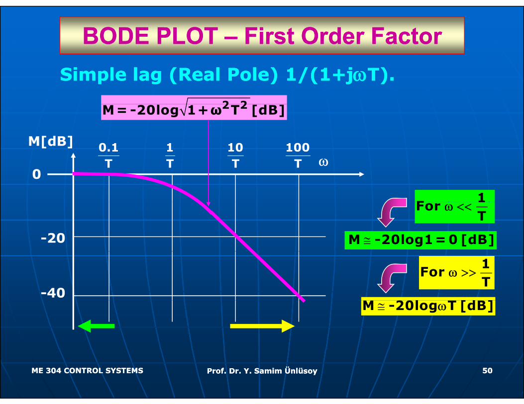
BODE PLOT BODE PLOT –– First Order FactorFirst Order FactorSimple lag (Real Pole) 1/(1+jSimple lag (Real Pole) 1/(1+jωωT).T).
2 22 2M= -20log 1+ω T [dB]
M[dB] 0.1 1 10 100
1F
ω0
T T T T
1For
Tω <<
-20 ≅M -20log1= 0 [dB]
1For
Tω >>
-40l [d ]≅M -20log T [dB]ω
ME 304 CONTROL SYSTEMSME 304 CONTROL SYSTEMS Prof. Dr. Y. Samim ÜnlüsoyProf. Dr. Y. Samim Ünlüsoy 5050
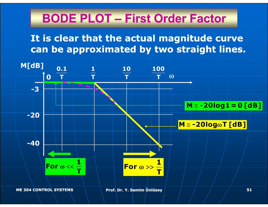
BODE PLOT BODE PLOT –– First Order FactorFirst Order FactorIt is clear that the actual magnitude curve It is clear that the actual magnitude curve can be approximated by two straight lines.can be approximated by two straight lines.pp y gpp y g
M[dB]ω0
0.1T
1T
10T
100T0
-3
T T T T
M 20l 1 0 [dB]-20
≅M -20log1= 0 [dB]
≅M -20log T [dB]ω
-40
1For
Tω << 1
For T
ω >>
ME 304 CONTROL SYSTEMSME 304 CONTROL SYSTEMS Prof. Dr. Y. Samim ÜnlüsoyProf. Dr. Y. Samim Ünlüsoy 5151
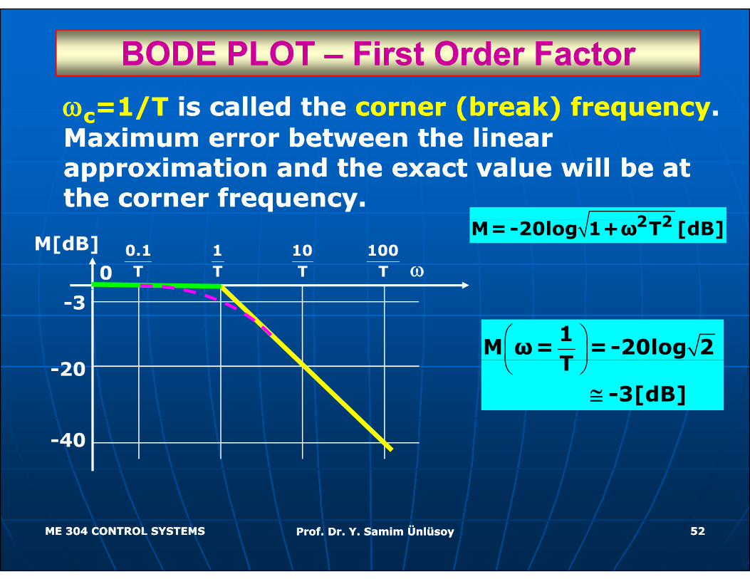
BODE PLOT BODE PLOT –– First Order FactorFirst Order Factorωωcc=1/T=1/T is called the is called the corner (break) frequencycorner (break) frequency. . Maximum error between the linear Maximum error between the linear approximation and the exact value will be at approximation and the exact value will be at the corner frequency.the corner frequency.
2 22 2M=-20log 1+ω T [dB]M[dB]
ω00.1T
1T
10T
100T
-3
⎛ ⎞⎜ ⎟⎝ ⎠
1M ω= =-20log 2
T-20⎜ ⎟⎝ ⎠T
-3[dB]≅
-40
ME 304 CONTROL SYSTEMSME 304 CONTROL SYSTEMS Prof. Dr. Y. Samim ÜnlüsoyProf. Dr. Y. Samim Ünlüsoy 5252
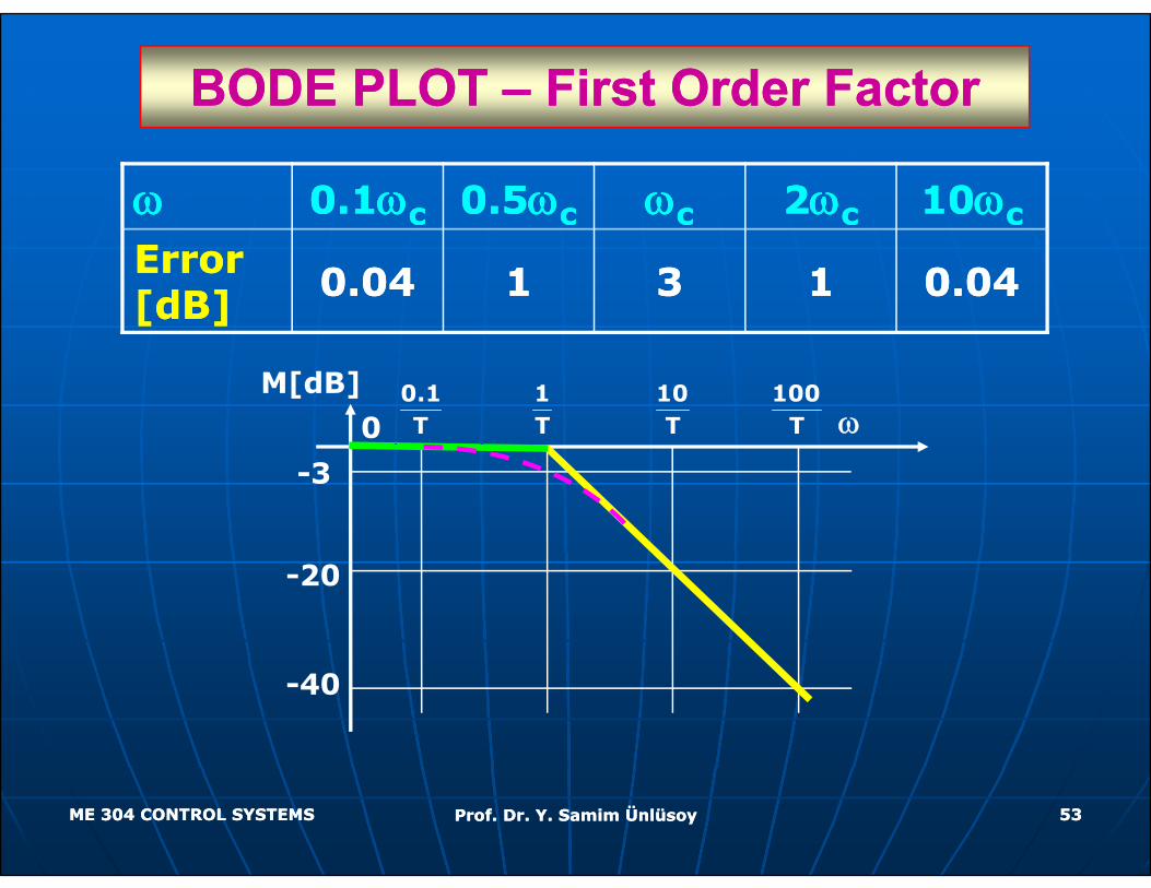
BODE PLOT BODE PLOT –– First Order FactorFirst Order Factor
ωω 0.10.1ωωcc 0.50.5ωωcc ωωcc 22ωωcc 1010ωωcc
Error Error [dB][dB] 0.040.04 11 33 11 0.040.04
M[dB]ω0
0.1T
1T
10T
100T
-3
-20
-40
ME 304 CONTROL SYSTEMSME 304 CONTROL SYSTEMS Prof. Dr. Y. Samim ÜnlüsoyProf. Dr. Y. Samim Ünlüsoy 5353
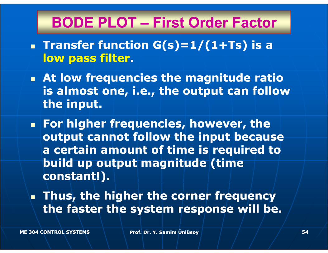
BODE PLOT BODE PLOT –– First Order FactorFirst Order FactorTransfer function G(s)=1/(1+Ts) is a Transfer function G(s)=1/(1+Ts) is a low pass filterlow pass filter..
At low frequencies the magnitude ratio At low frequencies the magnitude ratio is almost one, i.e., the output can follow is almost one, i.e., the output can follow , , p, , pthe input.the input.
For higher frequencies, however, the For higher frequencies, however, the For higher frequencies, however, the For higher frequencies, however, the output cannot follow the input because output cannot follow the input because a certain amount of time is required to a certain amount of time is required to build up output magnitude (time build up output magnitude (time constant!).constant!).
Thus, the higher the corner frequency Thus, the higher the corner frequency the faster the system response will be.the faster the system response will be.
ME 304 CONTROL SYSTEMSME 304 CONTROL SYSTEMS Prof. Dr. Y. Samim ÜnlüsoyProf. Dr. Y. Samim Ünlüsoy 5454
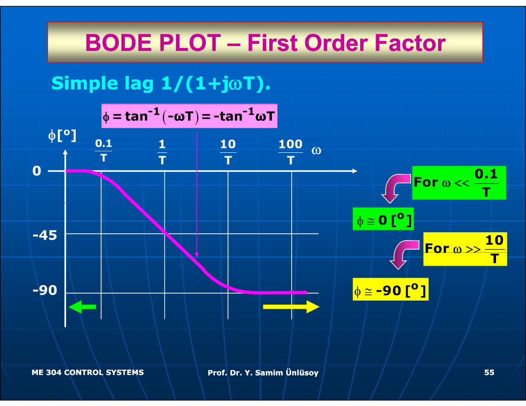
BODE PLOT BODE PLOT –– First Order FactorFirst Order FactorSimple lag 1/(1+jSimple lag 1/(1+jωωT).T).
( )-1 -1= tan -ωT =-tan ωTφ
ω0.1φ[o]
1 10 100
0.1For
Tω <<
ωT
0T T T
10For ω >>
φ ≅ o0 [ ]-45
For T
ω >>
φ ≅ o-90 [ ]-90
ME 304 CONTROL SYSTEMSME 304 CONTROL SYSTEMS Prof. Dr. Y. Samim ÜnlüsoyProf. Dr. Y. Samim Ünlüsoy 5555
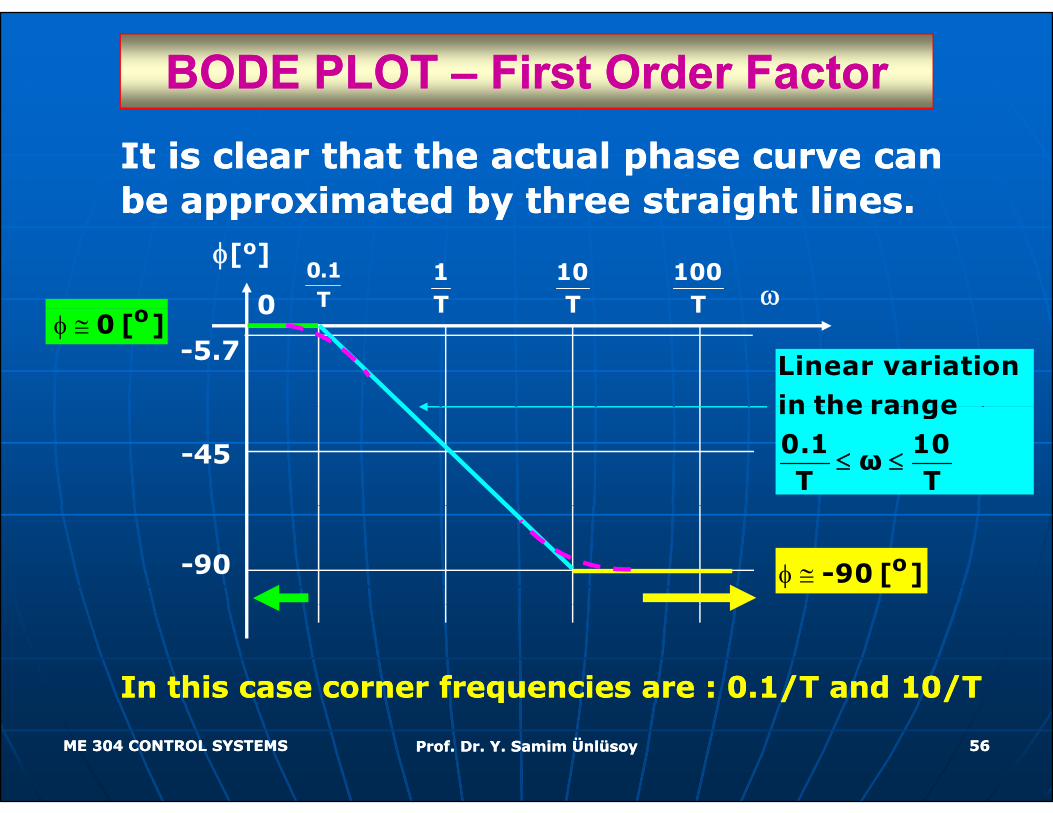
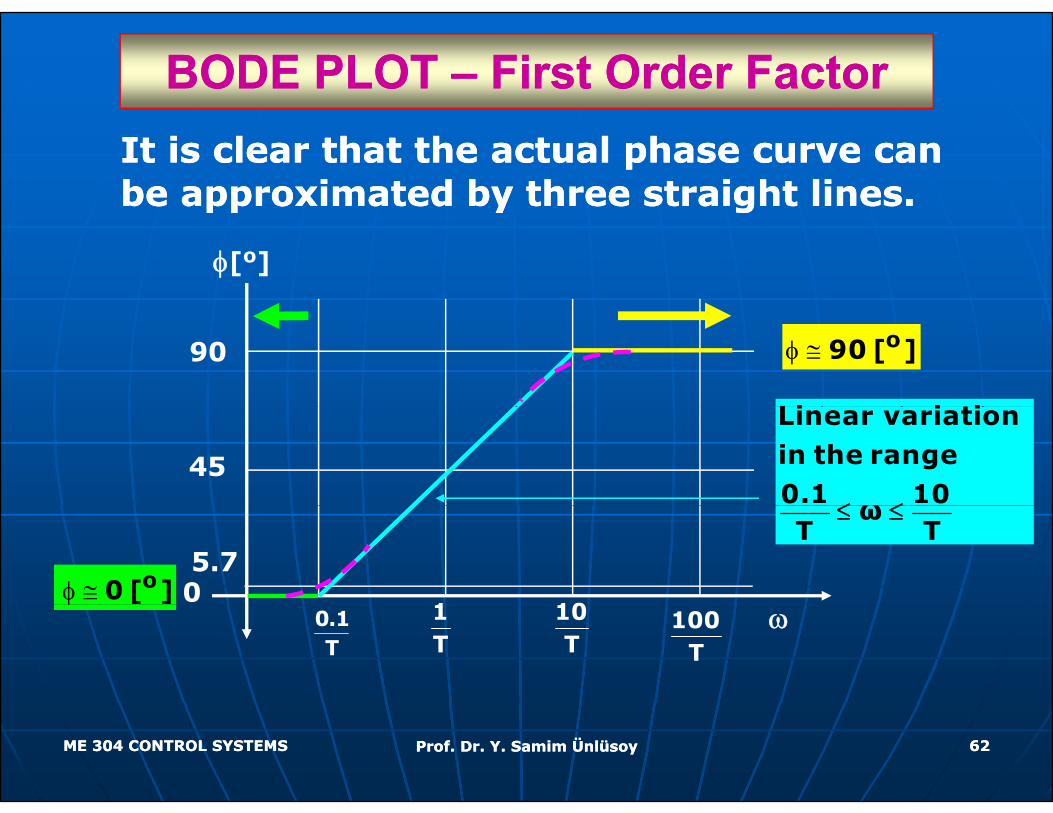
BODE PLOT BODE PLOT –– First Order FactorFirst Order FactorIt is clear that the actual phase curve can It is clear that the actual phase curve can be approximated by three straight lines.be approximated by three straight lines.be approximated by three straight lines.be approximated by three straight lines.
ω0.1T
φ[o]
01T
10T
100T
φ ≅ o0 [ ]0
-5.7
T T T
Linear variationin the range
-45
in the range0.1 10
ωT T
≤ ≤
φ ≅ o-90 [ ]-90
In this case corner frequencies are : 0.1/T and 10/TIn this case corner frequencies are : 0.1/T and 10/T
ME 304 CONTROL SYSTEMSME 304 CONTROL SYSTEMS Prof. Dr. Y. Samim ÜnlüsoyProf. Dr. Y. Samim Ünlüsoy 5656
BODE PLOT BODE PLOT –– First Order FactorFirst Order Factor
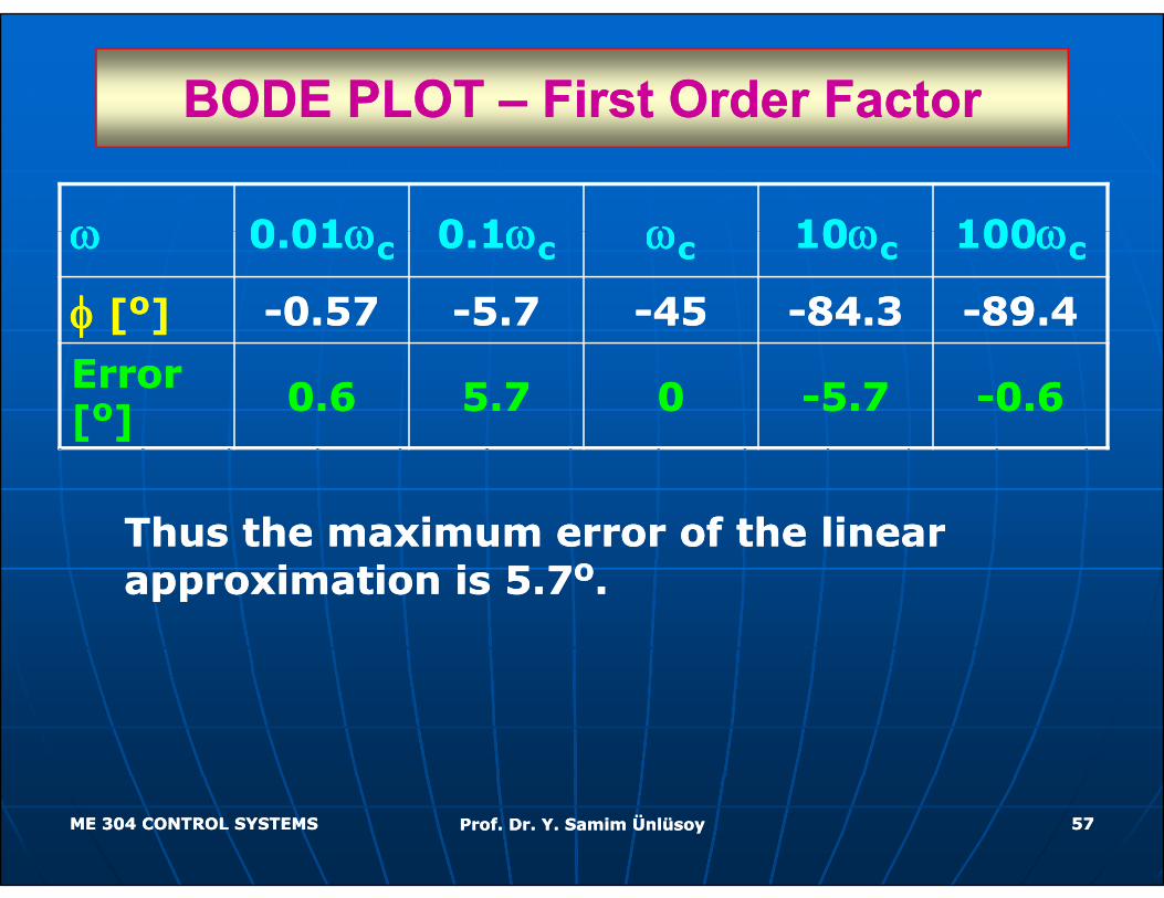
ωω 0 010 01ωω 0 10 1ωω ωω 1010ωω 100100ωωωω 0.010.01ωωcc 0.10.1ωωcc ωωcc 1010ωωcc 100100ωωcc
φφ [[oo]] --0.570.57 --5.75.7 --4545 --84.384.3 --89.489.4
Error Error [[oo]] 0.60.6 5.75.7 00 --5.75.7 --0.60.6
Thus the maximum error of the linear Thus the maximum error of the linear approximation is 5.7approximation is 5.7oo..
ME 304 CONTROL SYSTEMSME 304 CONTROL SYSTEMS Prof. Dr. Y. Samim ÜnlüsoyProf. Dr. Y. Samim Ünlüsoy 5757
BODE PLOT BODE PLOT –– First Order FactorFirst Order Factor
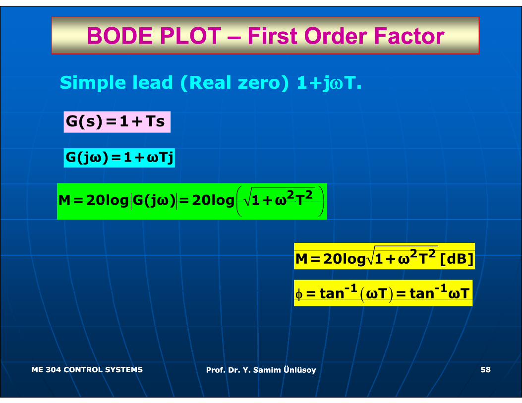
Simple lead (Real zero) 1+jSimple lead (Real zero) 1+jωωT.T.
G(s)=1+Ts
G(j ) 1 Tj
⎛ ⎞⎜ ⎟
2 2M=20log G(jω)=20log 1+ω T
G(jω)=1+ωTj
⎜ ⎟⎝ ⎠
M=20log G(jω)=20log 1+ω T
2 2
( )-1 -1= tan ωT = tan ωTφ
2 2M=20log 1+ω T [dB]
( )φ
ME 304 CONTROL SYSTEMSME 304 CONTROL SYSTEMS Prof. Dr. Y. Samim ÜnlüsoyProf. Dr. Y. Samim Ünlüsoy 5858
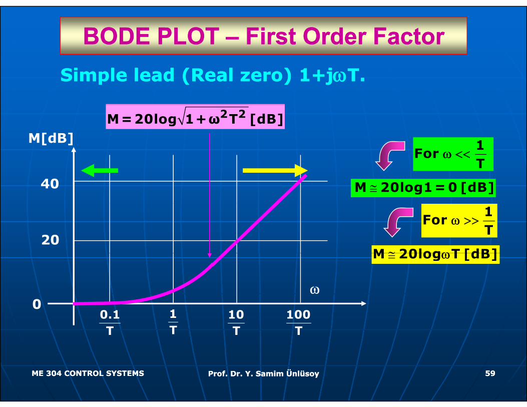
BODE PLOT BODE PLOT –– First Order FactorFirst Order FactorSimple lead (Real zero) 1+jSimple lead (Real zero) 1+jωωT.T.
2 2M=20log 1+ω T [dB]
1For ω <<
M[dB]For
Tω <<
≅M 20log1= 0 [dB]40
1For
Tω >>
≅M 20log T [dB]ω20
≅M 20log T [dB]ω
ω00
0.1T
1T
10T
100T
ME 304 CONTROL SYSTEMSME 304 CONTROL SYSTEMS Prof. Dr. Y. Samim ÜnlüsoyProf. Dr. Y. Samim Ünlüsoy 5959
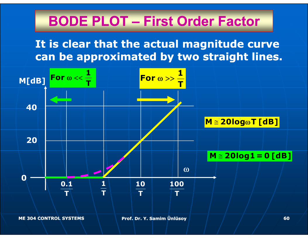
BODE PLOT BODE PLOT –– First Order FactorFirst Order FactorIt is clear that the actual magnitude curve It is clear that the actual magnitude curve can be approximated by two straight lines.can be approximated by two straight lines.pp y gpp y g
1For
Tω << 1
For T
ω >>M[dB]
M 20l T [dB]
40
≅M 20log T [dB]ω
20
≅M 20log1= 0 [dB]
ω00
0.1T
1T
10T
100T
ME 304 CONTROL SYSTEMSME 304 CONTROL SYSTEMS Prof. Dr. Y. Samim ÜnlüsoyProf. Dr. Y. Samim Ünlüsoy 6060
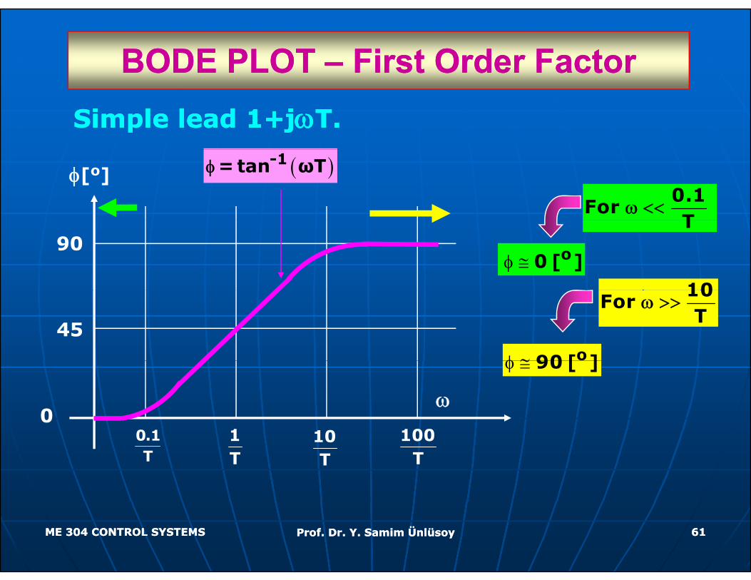
BODE PLOT BODE PLOT –– First Order FactorFirst Order FactorSimple lead 1+jSimple lead 1+jωωT.T.
0.1For
Tω <<
( )-1= tan ωTφφ[o]
T
10
φ ≅ o0 [ ]90
10For
Tω >>
φ ≅ o90 [ ]
45
φ ≅ 90 [ ]
ω
0 10
1 10 1000.1T
1T
10T
100T
ME 304 CONTROL SYSTEMSME 304 CONTROL SYSTEMS Prof. Dr. Y. Samim ÜnlüsoyProf. Dr. Y. Samim Ünlüsoy 6161
BODE PLOT BODE PLOT –– First Order FactorFirst Order FactorIt is clear that the actual phase curve can It is clear that the actual phase curve can be approximated by three straight lines.be approximated by three straight lines.pp y gpp y g
φ[o]
φ ≅ o90 [ ]90
Li i ti
45
Linear variationin the range0.1 10
ω≤ ≤
φ ≅ o0 [ ] 05.7
1 10
ωT T
≤ ≤
φω0.1
T
1T
10T
100T
ME 304 CONTROL SYSTEMSME 304 CONTROL SYSTEMS Prof. Dr. Y. Samim ÜnlüsoyProf. Dr. Y. Samim Ünlüsoy 6262
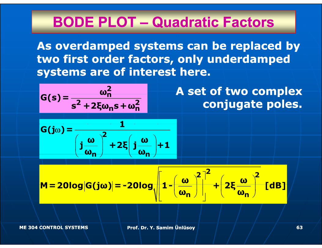
BODE PLOT BODE PLOT –– Quadratic FactorsQuadratic FactorsAs overdamped systems can be replaced by As overdamped systems can be replaced by two first order factors, only underdamped two first order factors, only underdamped , y p, y psystems are of interest here.systems are of interest here.
A set of two complex A set of two complex 2nω A set of two complex A set of two complex
conjugate poles.conjugate poles.n
2 2n n
ωG(s)=
s +2ξω s+ω
1
⎛ ⎞ ⎛ ⎞⎜ ⎟ ⎜ ⎟⎝ ⎠ ⎝ ⎠
2
n n
1G(j )=
ω ωj +2ξ j +1ω ω
ω
⎝ ⎠ ⎝ ⎠n nω ω
⎡ ⎤⎛ ⎞ ⎛ ⎞⎢ ⎥⎜ ⎟ ⎜ ⎟
22 2ω ω
M=20log G(jω) = 20log 1 + 2ξ [dB]⎢ ⎥⎜ ⎟ ⎜ ⎟⎢ ⎥⎝ ⎠ ⎝ ⎠⎣ ⎦n nM=20log G(jω) =-20log 1- + 2ξ [dB]
ω ω
ME 304 CONTROL SYSTEMSME 304 CONTROL SYSTEMS Prof. Dr. Y. Samim ÜnlüsoyProf. Dr. Y. Samim Ünlüsoy 6363
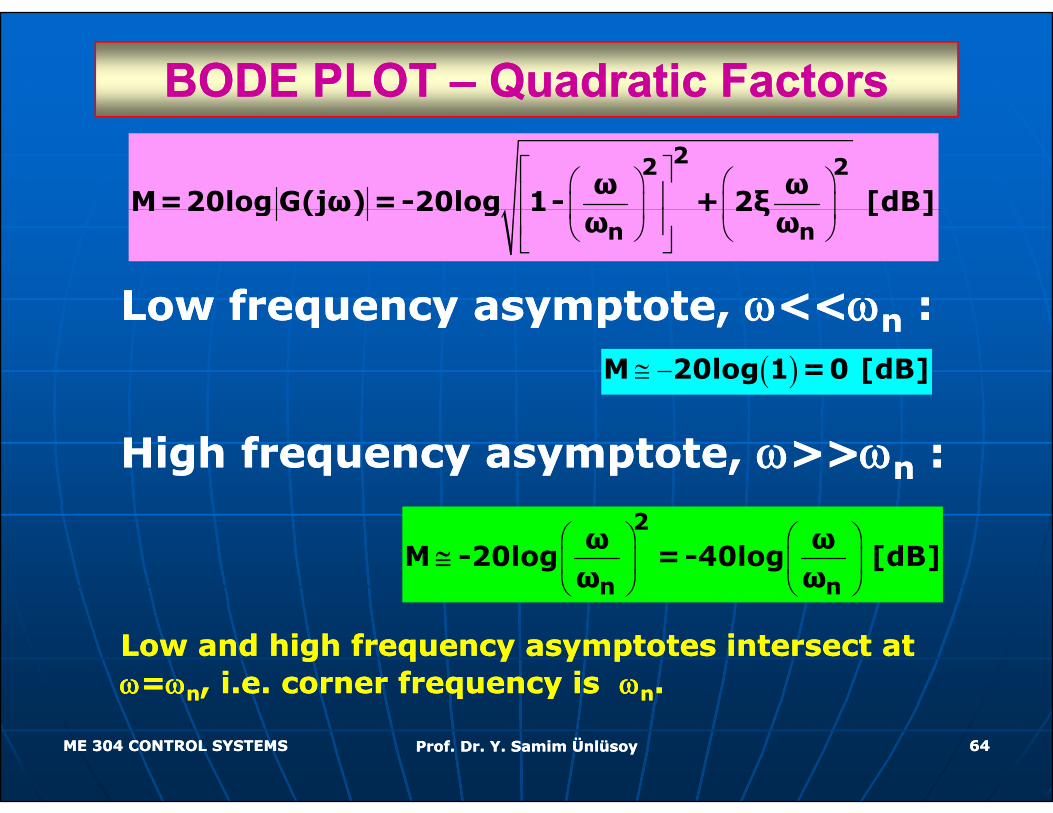
BODE PLOT BODE PLOT –– Quadratic FactorsQuadratic Factors
⎡ ⎤⎛ ⎞ ⎛ ⎞⎢ ⎥⎜ ⎟ ⎜ ⎟⎢ ⎥
22 2ω ω
M=20log G(jω) =-20log 1- + 2ξ [dB]⎜ ⎟ ⎜ ⎟⎢ ⎥⎝ ⎠ ⎝ ⎠⎣ ⎦n nM 20log G(jω) 20log 1 + 2ξ [dB]
ω ω
Low frequency asymptote Low frequency asymptote ωω<<<<ωω ::Low frequency asymptote, Low frequency asymptote, ωω<<<<ωωnn ::( )≅ −M 20log 1 =0 [dB]
High frequency asymptote, High frequency asymptote, ωω>>>>ωωnn ::
⎛ ⎞ ⎛ ⎞⎜ ⎟ ⎜ ⎟⎝ ⎠ ⎝ ⎠
2
n n
ω ωM -20log =-40log [dB]
ω ω≅
Low and high frequency asymptotes intersect at Low and high frequency asymptotes intersect at ωω==ωωnn, i.e. corner frequency is , i.e. corner frequency is ωωnn. .
ME 304 CONTROL SYSTEMSME 304 CONTROL SYSTEMS Prof. Dr. Y. Samim ÜnlüsoyProf. Dr. Y. Samim Ünlüsoy 6464
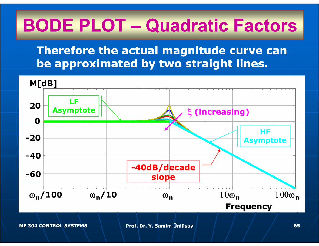
BODE PLOT BODE PLOT –– Quadratic FactorsQuadratic FactorsTherefore the actual magnitude curve can Therefore the actual magnitude curve can be approximated by two straight linesbe approximated by two straight lines
M[dB]
be approximated by two straight lines.be approximated by two straight lines.
ξ (increasing)20
0
LF Asymptote
0
-20
40
HF Asymptote
-40dB/decade slope
-40
-60
ωn 10ωn 100ωnωn/10ωn/100Frequency
ME 304 CONTROL SYSTEMSME 304 CONTROL SYSTEMS Prof. Dr. Y. Samim ÜnlüsoyProf. Dr. Y. Samim Ünlüsoy 6565
BODE PLOT BODE PLOT –– Quadratic FactorsQuadratic Factors
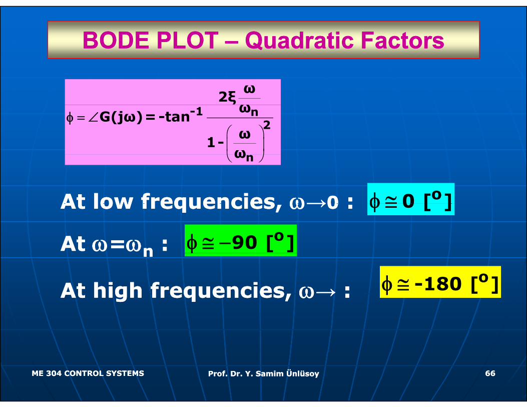
ω2ξω
⎛ ⎞⎜ ⎟⎝ ⎠
-1 n2
ωG(jω)=-tan
ω1-
ω
φ = ∠
⎝ ⎠nω
At low frequencies At low frequencies ωω→→00 :: o0 [ ]φ ≅At low frequencies, At low frequencies, ωω→→00 ::
At At ωω==ωωnn ::
0 [ ]φ ≅
o90 [ ]φ ≅ −nn
At high frequencies, At high frequencies, ωω→→ ::
φ
o-180 [ ]φ ≅
ME 304 CONTROL SYSTEMSME 304 CONTROL SYSTEMS Prof. Dr. Y. Samim ÜnlüsoyProf. Dr. Y. Samim Ünlüsoy 6666
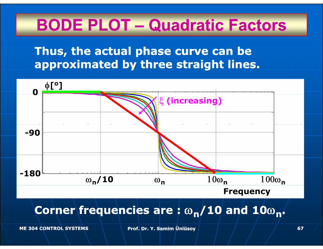
BODE PLOT BODE PLOT –– Quadratic FactorsQuadratic FactorsThus, the actual phase curve can be Thus, the actual phase curve can be approximated by three straight linesapproximated by three straight linesapproximated by three straight lines.approximated by three straight lines.
φ[o]0
ξ (increasing)0
-90o/decade slope
-90
ωn 10ωn 100ωnωn/10-180
Corner frequencies are : Corner frequencies are : ωωnn/10 and 10/10 and 10ωωnn. .
Frequency
ME 304 CONTROL SYSTEMSME 304 CONTROL SYSTEMS Prof. Dr. Y. Samim ÜnlüsoyProf. Dr. Y. Samim Ünlüsoy 6767
qq nn// nn
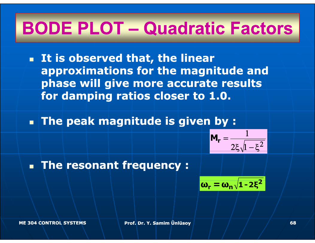
BODE PLOTBODE PLOT –– Quadratic FactorsQuadratic FactorsBODE PLOT BODE PLOT Quadratic FactorsQuadratic FactorsIt is observed that, the linear It is observed that, the linear ,,approximations for the magnitude and approximations for the magnitude and phase will give more accurate results phase will give more accurate results f d i i l 1 0f d i i l 1 0for damping ratios closer to 1.0.for damping ratios closer to 1.0.
The peak magnitude is given by :The peak magnitude is given by :The peak magnitude is given by :The peak magnitude is given by :
rΜ 21=
2ξ 1− ξ
The resonant frequency :The resonant frequency :
ξ ξ
22r n 1-2ξω =ω
ME 304 CONTROL SYSTEMSME 304 CONTROL SYSTEMS Prof. Dr. Y. Samim ÜnlüsoyProf. Dr. Y. Samim Ünlüsoy 6868
BODE PLOTBODE PLOT –– Quadratic FactorsQuadratic FactorsBODE PLOT BODE PLOT Quadratic FactorsQuadratic Factors
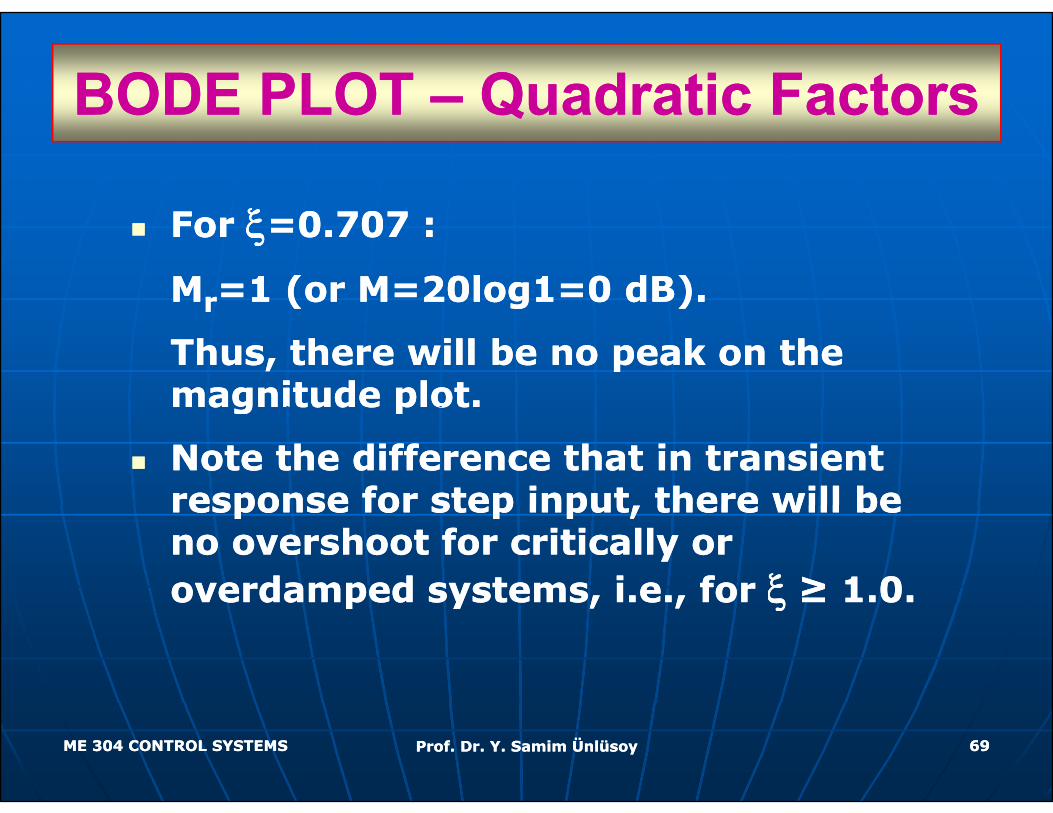
ξξFor For ξξ=0.707 :=0.707 :
MMrr=1 (or M=20log1=0 dB).=1 (or M=20log1=0 dB).rr ( g )( g )
Thus, there will be no peak on the Thus, there will be no peak on the magnitude plot.magnitude plot.magnitude plot.magnitude plot.
Note the difference that in transient Note the difference that in transient response for step input there will be response for step input there will be response for step input, there will be response for step input, there will be no overshoot for critically or no overshoot for critically or overdamped systems, i.e., for overdamped systems, i.e., for ξ ξ ≥ 1.0.≥ 1.0.p y , ,p y , , ξξ
ME 304 CONTROL SYSTEMSME 304 CONTROL SYSTEMS Prof. Dr. Y. Samim ÜnlüsoyProf. Dr. Y. Samim Ünlüsoy 6969
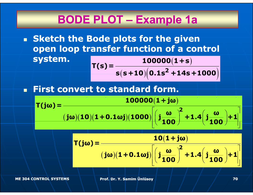
BODE PLOT BODE PLOT –– Example 1aExample 1aSketch the Bode plots for the given Sketch the Bode plots for the given open loop transfer function of a control open loop transfer function of a control open loop transfer function of a control open loop transfer function of a control system.system. ( )
( )( )2
100000 1+sT(s)=
s s+10 0 1s +14s+1000
First convert to standard form.First convert to standard form.
( )( )s s+10 0.1s +14s+1000
( )( )
( )( )( )( )⎡ ⎤⎛ ⎞ ⎛ ⎞⎢ ⎥⎜ ⎟ ⎜ ⎟⎝ ⎠ ⎝ ⎠⎢ ⎥
2
100000 1+jωT(jω)=
ω ωjω 10 1+0.1ωj 1000 j +1.4 j +1
100 100( )( )( )( ) ⎜ ⎟ ⎜ ⎟
⎝ ⎠ ⎝ ⎠⎢ ⎥⎣ ⎦100 100
( )⎡ ⎤
10 1+jωT(jω)=
( )( )⎡ ⎤⎛ ⎞ ⎛ ⎞⎢ ⎥⎜ ⎟ ⎜ ⎟⎝ ⎠ ⎝ ⎠⎢ ⎥⎣ ⎦
2T(jω)
ω ωjω 1+0.1ωj j +1.4 j +1
100 100
ME 304 CONTROL SYSTEMSME 304 CONTROL SYSTEMS Prof. Dr. Y. Samim ÜnlüsoyProf. Dr. Y. Samim Ünlüsoy 7070
BODE PLOT BODE PLOT –– Example 1bExample 1b( )
( )( )⎡ ⎤⎛ ⎞ ⎛ ⎞⎢ ⎥⎜ ⎟ ⎜ ⎟
2
10 1+jωT(jω)=
ω ωjω 1+0 1ωj j +1 4 j +1
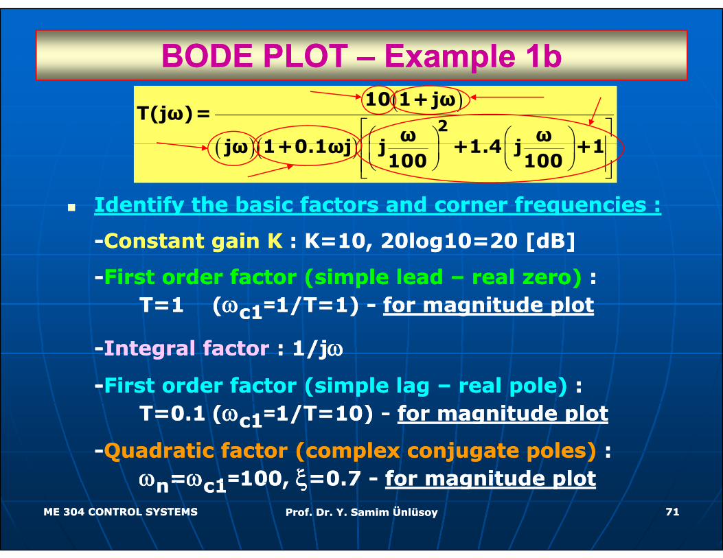
Identify the basic factors and corner frequencies :Identify the basic factors and corner frequencies :
( )( ) ⎛ ⎞ ⎛ ⎞⎢ ⎥⎜ ⎟ ⎜ ⎟⎝ ⎠ ⎝ ⎠⎢ ⎥⎣ ⎦
jω 1+0.1ωj j +1.4 j +1100 100
Identify the basic factors and corner frequencies :Identify the basic factors and corner frequencies :
--Constant gain KConstant gain K : K=10, 20log10=20 [dB]: K=10, 20log10=20 [dB]
--First order factor (simple lead First order factor (simple lead –– real zero)real zero) ::First order factor (simple lead First order factor (simple lead real zero)real zero) ::T=1T=1 ((ωωc1c1==1/T=1) 1/T=1) -- for magnitude plotfor magnitude plot
Integral factorIntegral factor : 1/j: 1/jωω--Integral factorIntegral factor : 1/j: 1/jωω
--First order factor (simple lag First order factor (simple lag –– real pole)real pole) : : T=0 1T=0 1 ((ωω 11==1/T=10) 1/T=10) -- for magnitude plotfor magnitude plotT=0.1T=0.1 ((ωωc1c1==1/T=10) 1/T=10) -- for magnitude plotfor magnitude plot
--Quadratic factor (complex conjugate poles)Quadratic factor (complex conjugate poles) ::ωωnn==ωωc1c1==100, 100, ξξ=0.7 =0.7 -- for magnitude plotfor magnitude plot
ME 304 CONTROL SYSTEMSME 304 CONTROL SYSTEMS Prof. Dr. Y. Samim ÜnlüsoyProf. Dr. Y. Samim Ünlüsoy 7171
ωωnn==ωωc1c1 100, 100, ξξ=0.7 =0.7 for magnitude plotfor magnitude plot
BODE PLOT BODE PLOT –– Example 1cExample 1c( )
( )( )⎡ ⎤⎛ ⎞ ⎛ ⎞⎢ ⎥⎜ ⎟ ⎜ ⎟
2
10 1+jωT(jω)=
ω ωjω 1+0 1ωj j +1 4 j +1
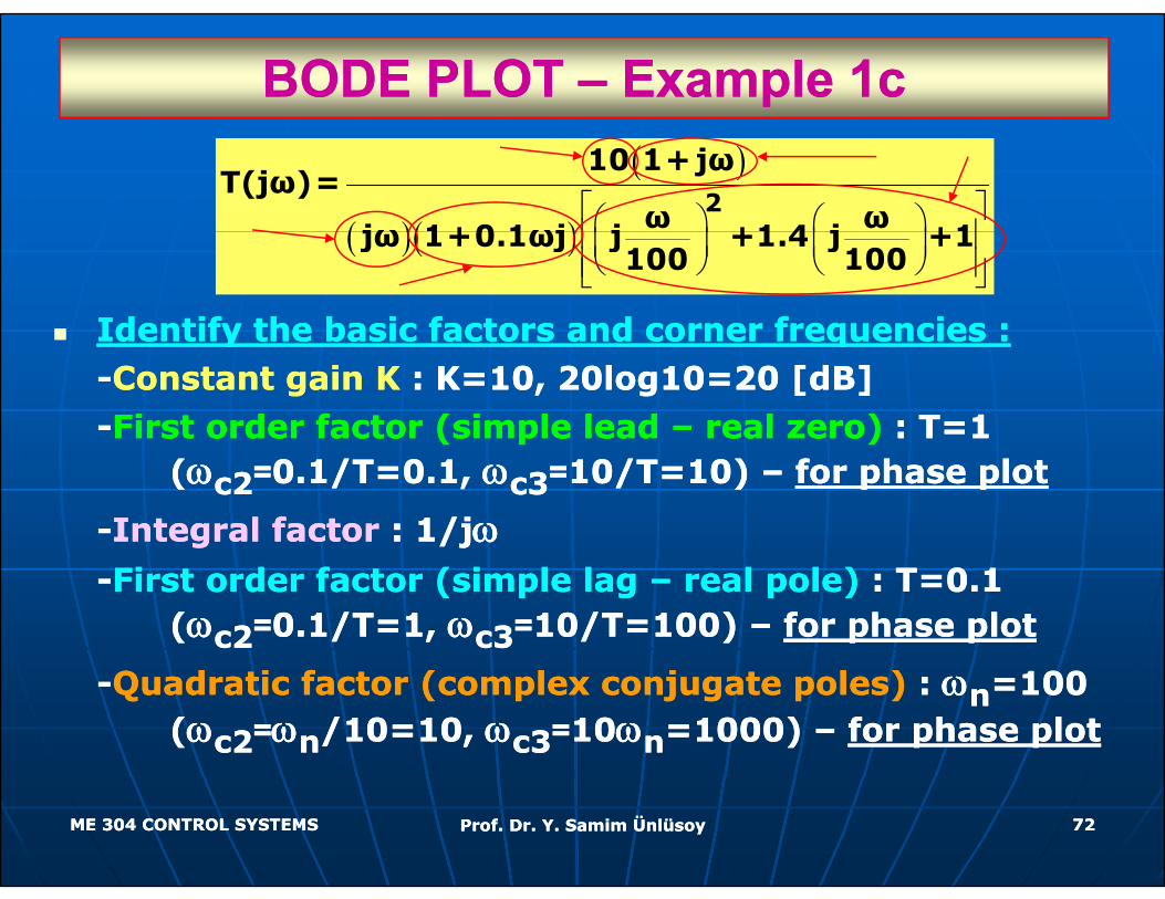
Identify the basic factors and corner frequencies :Identify the basic factors and corner frequencies :
( )( ) ⎛ ⎞ ⎛ ⎞⎢ ⎥⎜ ⎟ ⎜ ⎟⎝ ⎠ ⎝ ⎠⎢ ⎥⎣ ⎦
jω 1+0.1ωj j +1.4 j +1100 100
Identify the basic factors and corner frequencies :Identify the basic factors and corner frequencies :--Constant gain KConstant gain K : K=10, 20log10=20 [dB]: K=10, 20log10=20 [dB]--First order factor (simple lead First order factor (simple lead –– real zero)real zero) : T=1 : T=1
((ωωc2c2==0.1/T=0.1, 0.1/T=0.1, ωωc3c3==10/T=10) 10/T=10) –– for phase plotfor phase plot
--Integral factorIntegral factor : 1/j: 1/jωω--First order factor (simple lag First order factor (simple lag –– real pole)real pole) : T=0.1 : T=0.1
((ωωc2c2==0.1/T=1, 0.1/T=1, ωωc3c3==10/T=100) 10/T=100) –– for phase plotfor phase plot
--Quadratic factor (complex conjugate poles)Quadratic factor (complex conjugate poles) : : ωωnn=100 =100 ((ωωc2c2==ωωnn/10=10, /10=10, ωωc3c3==1010ωωnn=1000) =1000) –– for phase plotfor phase plot
ME 304 CONTROL SYSTEMSME 304 CONTROL SYSTEMS Prof. Dr. Y. Samim ÜnlüsoyProf. Dr. Y. Samim Ünlüsoy 7272
BODE PLOT BODE PLOT –– Example 1dExample 1d
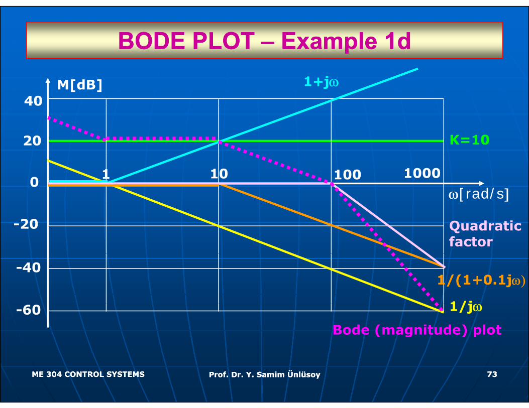
40M[dB] 1+jω
20
40
K=10
0 1 10 100 1000
ω[rad/s]
-20 Quadratic factor
-40
1/j
1/(1+0.1jω)
-60 1/jω
Bode (magnitude) plot
ME 304 CONTROL SYSTEMSME 304 CONTROL SYSTEMS Prof. Dr. Y. Samim ÜnlüsoyProf. Dr. Y. Samim Ünlüsoy 7373
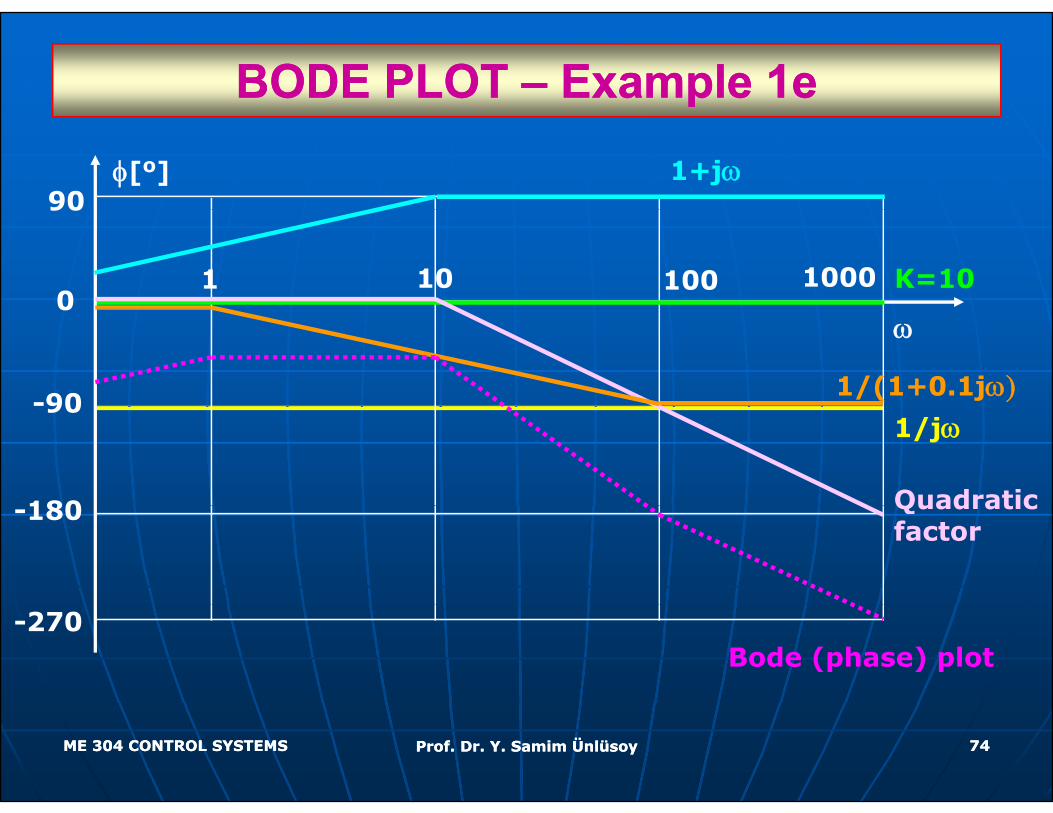
BODE PLOT BODE PLOT –– Example 1eExample 1e
90φ[o] 1+jω
0
90
1 10 100 1000 K=100
-90
ω
1/(1+0.1jω)90
180
1/jω
Quadratic -180 Quadratic factor
-270Bode (phase) plot
ME 304 CONTROL SYSTEMSME 304 CONTROL SYSTEMS Prof. Dr. Y. Samim ÜnlüsoyProf. Dr. Y. Samim Ünlüsoy 7474
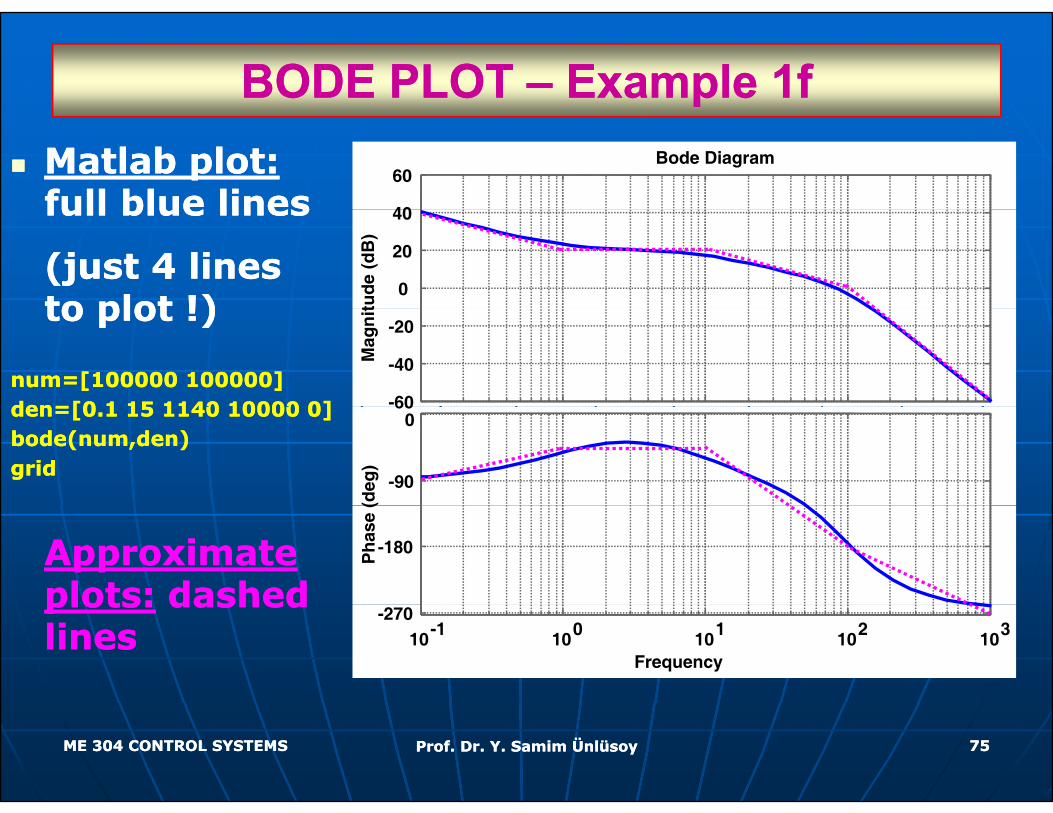
BODE PLOT BODE PLOT –– Example 1fExample 1fMatlab plot:Matlab plot:full blue linesfull blue lines 40
60Bode Diagram
full blue linesfull blue lines
(just 4 lines (just 4 lines to plot !)to plot !)
0
20
40
tud
e (d
B)
to plot !)to plot !)
num=[100000 100000]num=[100000 100000]den=[0 1 15 1140 10000 0]den=[0 1 15 1140 10000 0] -60
-40
-20
Mag
nit
den=[0.1 15 1140 10000 0]den=[0.1 15 1140 10000 0]bode(num,den)bode(num,den)gridgrid
60
-90
0
(deg
)
Approximate Approximate plots:plots: dashed dashed
-180
Ph
ase
(
plots:plots: dashed dashed lineslines 10-1 100 101 102 103
-270
Frequency
ME 304 CONTROL SYSTEMSME 304 CONTROL SYSTEMS Prof. Dr. Y. Samim ÜnlüsoyProf. Dr. Y. Samim Ünlüsoy 7575
STABILITY ANALYSISSTABILITY ANALYSISNise Sect 10 7 pp 638Nise Sect 10 7 pp 638--641641Nise Sect. 10.7, pp.638Nise Sect. 10.7, pp.638 641641
Transfer functions which have no poles or Transfer functions which have no poles or Transfer functions which have no poles or Transfer functions which have no poles or zeroes on the right hand side of the zeroes on the right hand side of the complex plane are called complex plane are called minimum phase minimum phase transfer funtions.transfer funtions.
Nonminimum phaseNonminimum phase transfer functions, on transfer functions, on pp ,,the other hand, have zeros and/or poles on the other hand, have zeros and/or poles on the right hand side of the complex plane. the right hand side of the complex plane.
The major disadvantage of Bode Plot is that The major disadvantage of Bode Plot is that stability of stability of onlyonly minimum phase systems minimum phase systems can can be determined using Bode plot.be determined using Bode plot.
ME 304 CONTROL SYSTEMSME 304 CONTROL SYSTEMS Prof. Dr. Y. Samim ÜnlüsoyProf. Dr. Y. Samim Ünlüsoy 7676
STABILITY ANALYSISSTABILITY ANALYSIS
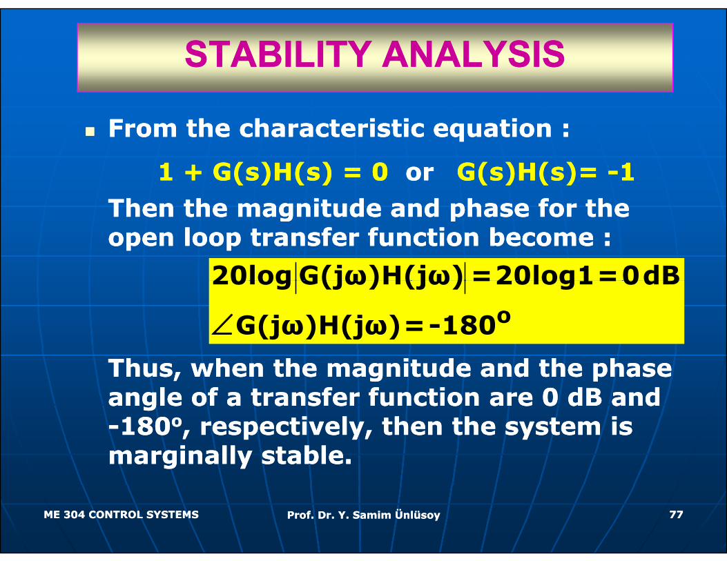
From the characteristic equation :From the characteristic equation :
1 + G(s)H(s) = 01 + G(s)H(s) = 0 oror G(s)H(s)= G(s)H(s)= --11Then the magnitude and phase for the Then the magnitude and phase for the Then the magnitude and phase for the Then the magnitude and phase for the open loop transfer function become :open loop transfer function become :
20log G(jω)H(jω) =20log1=0dBo
20log G(jω)H(jω) =20log1=0dB
G(jω)H(jω)=-180∠Thus, when the magnitude and the phase Thus, when the magnitude and the phase angle of a transfer function are 0 dB and angle of a transfer function are 0 dB and
8080 i l h h ii l h h i--180180oo, respectively, then the system is , respectively, then the system is marginally stable. marginally stable.
ME 304 CONTROL SYSTEMSME 304 CONTROL SYSTEMS Prof. Dr. Y. Samim ÜnlüsoyProf. Dr. Y. Samim Ünlüsoy 7777
STABILITY ANALSISSTABILITY ANALSIS
If at the frequency, for which phase If at the frequency, for which phase becomes equal to becomes equal to --180180oo, gain is below 0 , gain is below 0 dB, then the system is stable (unstable dB, then the system is stable (unstable otherwise)otherwise)otherwise).otherwise).
Further, if at the frequency, for which Further, if at the frequency, for which i b l t h i i b l t h i gain becomes equal to zero, phase is gain becomes equal to zero, phase is
above above --180180oo, then the system is stable , then the system is stable (unstable otherwise)(unstable otherwise)(unstable otherwise).(unstable otherwise).
Thus, Thus, relative stabilityrelative stability of a minimum of a minimum phase system can be determined phase system can be determined phase system can be determined phase system can be determined according to these observations.according to these observations.
ME 304 CONTROL SYSTEMSME 304 CONTROL SYSTEMS Prof. Dr. Y. Samim ÜnlüsoyProf. Dr. Y. Samim Ünlüsoy 7878
GAIN and PHASE MARGINSGAIN and PHASE MARGINSNi 638Ni 638 641641Nise pp. 638Nise pp. 638--641641
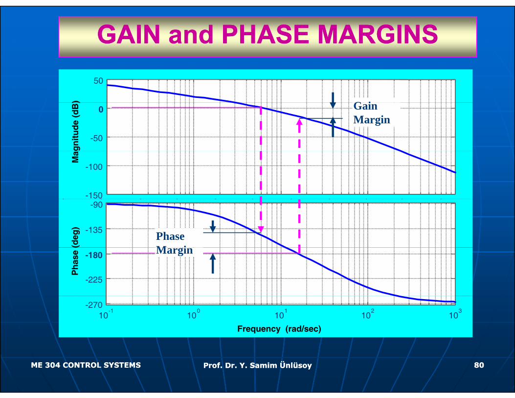
Gain Margin :Gain Margin : Additional gain to make Additional gain to make Gain Margin :Gain Margin : Additional gain to make Additional gain to make the system marginally stable at a the system marginally stable at a frequency for which the phase of the frequency for which the phase of the q y pq y popen loop transfer function passes open loop transfer function passes through through --180180oo..
Phase Margin :Phase Margin : Additional phase angle Additional phase angle to make the system marginally stable at to make the system marginally stable at a frequency for which the magnitude of a frequency for which the magnitude of the open loop transfer function is 0 dB.the open loop transfer function is 0 dB.
ME 304 CONTROL SYSTEMSME 304 CONTROL SYSTEMS Prof. Dr. Y. Samim ÜnlüsoyProf. Dr. Y. Samim Ünlüsoy 7979
GAIN and PHASE MARGINSGAIN and PHASE MARGINS50
) G i
-50
0
gn
itu
de
(dB
) Gain Margin
-150
-100
Mag
-135
-90
(deg
)
Phase M i
-225
-180
Ph
ase
( Margin
10-1
100
101
102
103
-270
Frequency (rad/sec)
ME 304 CONTROL SYSTEMSME 304 CONTROL SYSTEMS Prof. Dr. Y. Samim ÜnlüsoyProf. Dr. Y. Samim Ünlüsoy 8080
BODE PLOTBODE PLOTCan you Can you identify the identify the identify the identify the transfer transfer function function approximatelyapproximatelyif the if the meas red meas red measured measured Bode diagram Bode diagram is available ?is available ?is available ?is available ?
ME 304 CONTROL SYSTEMSME 304 CONTROL SYSTEMS Prof. Dr. Y. Samim ÜnlüsoyProf. Dr. Y. Samim Ünlüsoy 8181