CFD Simulation of Liquid-Solid Mechanically...

CFD Simulation of Liquid-Solid Mechanically Agitated Contactor

68

4.1. Introduction

Mechanical agitation is the most widely used unit operation for liquid–solid

mixing in the chemical industries, mineral processing, wastewater treatment and

biochemical process industries. The typical process requirement in this type of reactor

is for the solid phase to be suspended for the purpose of dissolution, reaction, or to

provide feed uniformity. Since the suspension of solids is an intensive energy

consuming operation, the main challenge is the ability to maintain the solid

suspension at the lowest cost. The challenge is in understanding the fluid dynamics in

the reactor and relating this knowledge to design.

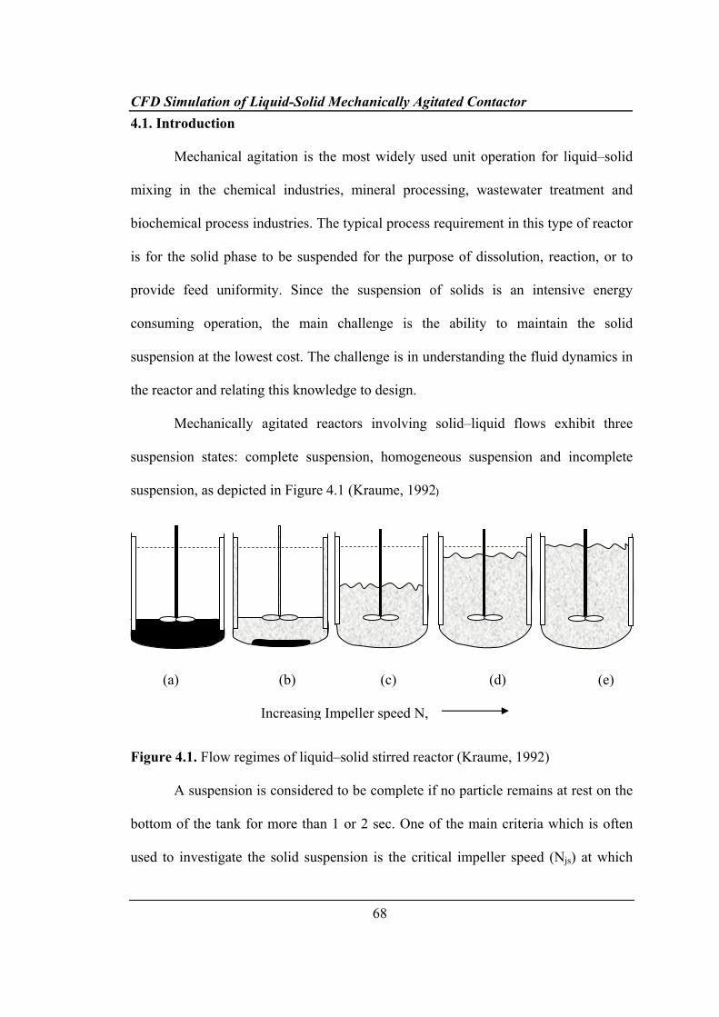
Mechanically agitated reactors involving solid–liquid flows exhibit three

suspension states: complete suspension, homogeneous suspension and incomplete

suspension, as depicted in Figure 4.1 (Kraume, 1992)

Figure 4.1. Flow regimes of liquid–solid stirred reactor (Kraume, 1992)

A suspension is considered to be complete if no particle remains at rest on the

bottom of the tank for more than 1 or 2 sec. One of the main criteria which is often

used to investigate the solid suspension is the critical impeller speed (Njs) at which

(a) (b) (c) (d) (e) Increasing Impeller speed N,


69

solids are just suspended (Zwietering, 1958). A homogeneous suspension is the state

of solid suspension, where the local solid concentration is constant throughout the

entire region of column. An incomplete suspension is the state, where the solids are

deposited at the bottom of reactor. Zwietering (1958) is the first author, who proposed

a correlation for the minimum impeller speed for complete suspension of solids on the

basis of dimensional analysis of the results obtained from over a thousand

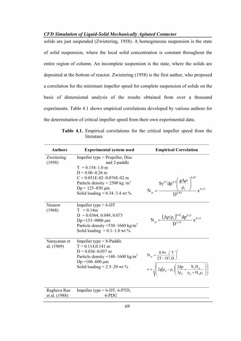
experiments. Table 4.1 shows empirical correlations developed by various authors for

the determination of critical impeller speed from their own experimental data.

Table 4.1. Empirical correlations for the critical impeller speed from the literature

Authors Experimental system used Empirical Correlation

Zweitering (1958)

Impeller type = Propeller, Disc and 2-paddle T = 0.154–1.0 m D = 0.06–0.26 m C = 0.051E-02–0.076E-02 m Particle density = 2500 kg /m3 Dp = 125–850 μm Solid loading = 0.34–3.4 wt %

0.130.85

0.45

l

0.20.1

js xD

ρgΔdpSγ

N⎟⎟⎠

⎞⎜⎜⎝

⎛

=

ρ

Nienow (1968)

Impeller type = 6-DT T = 0.14m D = 0.0364, 0.049, 0.073 Dp =153–9000 μm Particle density =530–1660 kg/m3 Solid loading = 0.1–1.0 wt %

( ) 0.12

2.25

0.210.43l

js xD

dpΔρ/ρN =

Narayanan et al. (1969)

Impeller type = 8-Paddle T = 0.114,0.141 m D = 0.036–0.057 m Particle density =140–1600 kg/m3 Dp =106–600 μm Solid loading = 2.5–20 wt %

( )⎟⎟⎠

⎞⎜⎜⎝

⎛⎟⎟⎠

⎞⎜⎜⎝

⎛

++−=

⎟⎠⎞

⎜⎝⎛

−=

lslp

sls

plp

2

js

ρHρHX

3ρ2dpρρ2gv

DT

D2T0.9vN

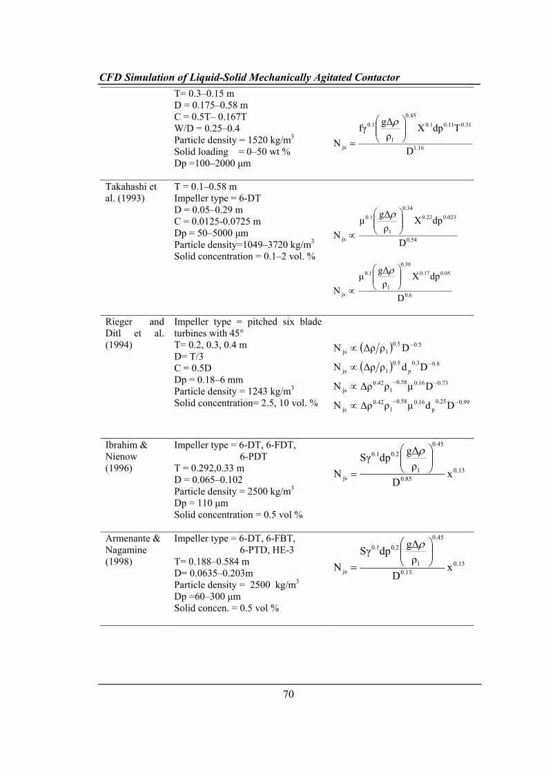
Raghava Rao et al. (1988)

Impeller type = 6-DT, 6-PTD, 6-PDU


70

T= 0.3–0.15 m D = 0.175–0.58 m C = 0.5T– 0.167T W/D = 0.25–0.4 Particle density = 1520 kg/m3 Solid loading = 0–50 wt % Dp =100–2000 μm

1.16

0.310.110.10.45

l

0.1

js D

TdpXρ

gΔfγN

⎟⎟⎠

⎞⎜⎜⎝

⎛

=

ρ

Takahashi et al. (1993)

T = 0.1–0.58 m Impeller type = 6-DT D = 0.05–0.29 m C = 0.0125-0.0725 m Dp = 50–5000 μm Particle density=1049–3720 kg/m3 Solid concentration = 0.1–2 vol. %

0.54

0.0230.220.34

l

0.1

js D

dpXρ

gΔμN

⎟⎟⎠

⎞⎜⎜⎝

⎛

∝

ρ

0.6

0.050.170.38

l

0.1

js D

dpXρ

gΔμN

⎟⎟⎠

⎞⎜⎜⎝

⎛

∝

ρ

Rieger and Ditl et al. (1994)

Impeller type = pitched six blade turbines with 45° T= 0.2, 0.3, 0.4 m D= T/3 C = 0.5D Dp = 0.18–6 mm Particle density = 1243 kg/m3 Solid concentration= 2.5, 10 vol. %

( )( )

0.990.25p

0.160.58l

0.42js

0.730.160.58l

0.42js

0.80.3p

0.5ljs

0.50.5ljs

DdμρΔρN

DμρΔρN

DdρΔρN

DρΔρN

−−

−−

−

−

∝

∝

∝

∝

Ibrahim & Nienow (1996)

Impeller type = 6-DT, 6-FDT, 6-PDT T = 0.292,0.33 m D = 0.065–0.102 Particle density = 2500 kg/m3 Dp = 110 μm Solid concentration = 0.5 vol %

0.130.85

0.45

l

0.20.1

js xD

ρgΔdpSγ

N⎟⎟⎠

⎞⎜⎜⎝

⎛

=

ρ

Armenante & Nagamine (1998)

Impeller type = 6-DT, 6-FBT, 6-PTD, HE-3 T= 0.188–0.584 m D= 0.0635–0.203m Particle density = 2500 kg/m3 Dp =60–300 μm Solid concen. = 0.5 vol %

0.130.13

0.45

l

0.20.1

js xD

ρgΔdpSγ

N⎟⎟⎠

⎞⎜⎜⎝

⎛

=

ρ


71

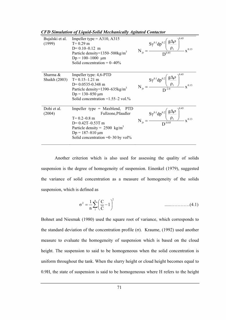
Bujalski et al. (1999)

Impeller type = A310, A315 T= 0.29 m D= 0.10–0.12 m Particle density=1350–500kg/m3 Dp = 100–1000 μm Solid concentration = 0–40%

0.1385.0

0.45

l

0.20.1

js xD

ρgΔdpSγ

N⎟⎟⎠

⎞⎜⎜⎝

⎛

=

ρ

Sharma & Shaikh (2003)

Impeller type: 4,6-PTD T= 0.15–1.21 m D= 0.0535-0.348 m Particle density=1390–635kg/m3 Dp = 130–850 μm Solid concentration =1.55–2 vol.%

0.132.0-

0.45

l

0.20.1

js xD

ρgΔdpSγ

N⎟⎟⎠

⎞⎜⎜⎝

⎛

=

ρ

Dohi et al. (2004)

Impeller type = Maxblend, PTD Fullzone,Pfaudler

T= 0.2–0.8 m D= 0.42T–0.53T m Particle density = 2500 kg/m3 Dp = 187–810 μm Solid concentration =0–30 by vol%

0.130.85-

0.45

l

0.20.1

js xD

ρgΔdpSγ

N⎟⎟⎠

⎞⎜⎜⎝

⎛

=

ρ

Another criterion which is also used for assessing the quality of solids

suspension is the degree of homogeneity of suspension. Einenkel (1979), suggested

the variance of solid concentration as a measure of homogeneity of the solids

suspension, which is defined as

2n

1

2 1CC

n1σ ∑ ⎟

⎠⎞

⎜⎝⎛ −= ......…………(4.1)

Bohnet and Niesmak (1980) used the square root of variance, which corresponds to

the standard deviation of the concentration profile (σ). Kraume, (1992) used another

measure to evaluate the homogeneity of suspension which is based on the cloud

height. The suspension to said to be homogeneous when the solid concentration is

uniform throughout the tank. When the slurry height or cloud height becomes equal to

0.9H, the state of suspension is said to be homogeneous where H refers to the height


72

of the reactor. Eventhough the suspended slurry height or cloud height is not an

absolute measure of homogeneity, it may be useful for comparing the identical

slurries.

During the last few decades, various models have been proposed for

quantifying the solid suspension from the theoretical power requirement. Kolar (1967)

presented a model for solid suspension based on energy balance, that all the power is

consumed for suspending the solids and that the stirred tank is hydrodynamically

homogeneous. Baldi et al. (1978) proposed a new model for complete suspension of

solids where it is assumed that the suspension of particles is due to turbulent eddies of

certain critical scale. Further it is assumed that the critical turbulent eddies that cause

the suspension of the particles being at rest on the tank bottom have a scale of the

order of the particles size, and the energy transferred by these eddies to the particles

is able to lift them at a height of the order of particle diameter. Since their hypothesis

related the energy dissipation rate for solid suspension to the average energy

dissipation in the vessel by employing modified Reynolds number concept, it gave

good insight into the suspension process compared to other approaches.

Chudacek (1986) proposed an alternative model for the homogeneous

suspension based on the equivalence of particle settling velocity and mean upward

flow velocity at the critical zone of the tank which leads to the constant impeller tip

speed criterion, but this is valid only under conditions of geometric and hydrodynamic

similarity. Shamlou and Koutsakos (1989) introduced a theoretical model based on

the fluid dynamics and the body force acting on solid particles at the state of incipient

motion and subsequent suspension. Rieger and Ditl (1994) developed a dimensionless


73

equation for the critical impeller speed required for complete suspension of solids

based on the inspection analysis of governing fluid dynamic equations. They observed

four different hydrodynamic regimes based on the relative particle size and Reynolds

number values.

Since most of the present knowledge on solid suspension is based on

simplified models and empirical correlations it cannot account for the complex

manner in which various parameters interact with the complex flow field. Eventhough

in the recent past, both invasive and non invasive experimental measurement

techniques have been reported in the literature, significant improvements of the design

capability and reliability can be expected from advances in computational fluid

dynamics (CFD) techniques (Dudukovic et al., 1999). CFD simulations offer the only

cost-effective means to acquire the detailed information on flow and turbulence fields

needed for realistic distributed-parameter process simulations. Table 4.2 shows the

various studies related to CFD modeling of solid suspension in such mechanically

agitated contactors in the recent past.

Hence, the objective of this work is to develop a validated CFD simulation

tool based on Eulerian multi-fluid approach for the prediction of the solid suspension

in a solid–liquid mechanically agitated contactor. CFD simulations are carried out

using the commercial package ANSYS CFX-10. After the validation, the CFD

simulations have been extended to study the effects of impeller design, impeller speed

and particle size on the solid suspension behavior.


74

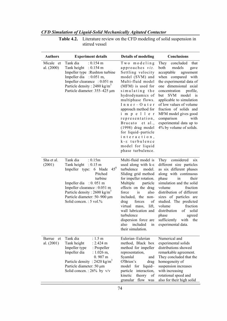
Table 4.2. Literature review on the CFD modeling of solid suspension in stirred vessel

Authors Experiment details Details of modeling Conclusions

Micale et al. (2000)

Tank dia : 0.154 m Tank height : 0.154 m Impeller type :Rushton turbine Impeller dia : 0.051 m, Impeller clearance : 0.051 m Particle density : 2480 kg/m3 Particle diameter: 355–425 μm

T w o m o d e l i n g a p p r o a c h e s v i z . Set t l ing veloci ty model (SVM) and Multi-fluid model (MFM) is used for s i m u l a t i n g t h e hydrodynamics of multiphase flows. I n n e r – O u t e r approach method for i m p e l l e r r e p r e s e n t a t i o n , B r u c a t o e t a l . , (1998) drag model for liquid–particle i n t e r a c t i o n , k - ε t u r b u l e n c e model for l iquid phase turbulence.

They concluded that both models gave acceptable agreement when compared with the experimental data of one dimensional axial concentration profile, but SVM model is applicable to simulation of low values of volume fraction of solids and MFM model gives good comparison with experimental data up to 4% by volume of solids.

Sha et al. (2001)

Tank dia : 0.15m Tank height : 0.15 m Impeller type: 6 blade 450

Pitched turbine

Impeller dia : 0. 051 m Impeller clearance : 0.051 m Particle density : 2600 kg/m3 Particle diameter: 50–900 μm Solid concen. : 5 vol.%

Multi-fluid model is used along with k-ε turbulence model. Sliding grid method for impeller rotation. Multiple particle effects on the drag force is also included, the non-drag forces of virtual mass, lift, wall lubrication and turbulence dispersion force are also included in their simulation.

They considered six different size particles as six different phases along with continuous phase in their simulation and the solid volume fraction distribution of different sizes of particles are studied. The predicted volume fraction distribution of solid phase agreed sufficiently with the experimental data.

Barrue et al. (2001)

Tank dia : 1.5 m Tank height : 2.424 m Impeller type : Propeller Impeller dia : 1.026 m, 0. 907 m Particle density : 2420 kg/m3 Particle diameter: 50 μm Solid concen. : 26% by v/v

Eulerian–Eulerian method, Black box method for impeller representation, Syamlal and O'Brien’s drag model for liquid–particle interaction, kinetic theory of granular flow was

Numerical and experimental solids distributions showed remarkable agreement. They concluded that the homogeneity of suspension increases with increasing rotational speed and also for their high solid


75

used for solid phase description, k-ε turbulence model for liquid phase turbulence.

concentration, increase of the mean concentration increases the homogeneity of the vessel.

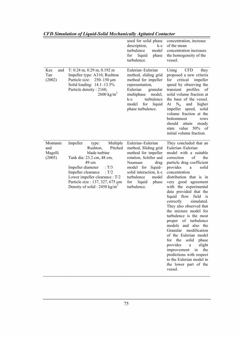
Kee and Tan (2002)

T: 0.24 m, 0.29 m, 0.192 m Impeller type: A310, Rushton Particle size: 250–150 μm Solid loading: 14.1–13.5% Particle density : 2160, 2600 kg/m3

Eulerian–Eulerian method, sliding grid method for impeller representation, Eulerian granular multiphase model, k-ε turbulence model for liquid phase turbulence.

Using CFD they proposed a new criteria for critical impeller speed by observing the transient profiles of solid volume fraction at the base of the vessel. At Njs and higher impeller speed, solid volume fraction at the bottommost rows should attain steady state value 50% of initial volume fraction.

Montante and Magelli (2005)

Impeller type: Multiple Rushton, Pitched blade turbine

Tank dia: 23.2 cm, 48 cm, 49 cm Impeller diameter : T/3 Impeller clearance : T/2 Lower impeller clearance : T/2 Particle size : 137, 327, 675 μm Density of solid : 2450 kg/m3

Eulerian–Eulerian method, Sliding grid method for impeller rotation, Schiller and Naumaan drag model for liquid–solid interaction, k-ε turbulence model for liquid phase turbulence.

They concluded that an Eulerian–Eulerian model with a suitable correction of the particle drag coefficient provides a solid concentration distribution that is in very good agreement with the experimental data provided that the liquid flow field is correctly simulated. They also observed that the mixture model for turbulence is the most proper of turbulence models and also the Granular modification of the Eulerian model for the solid phase provides a slight improvement in the predictions with respect to the Eulerian model in the lower part of the vessel.


76

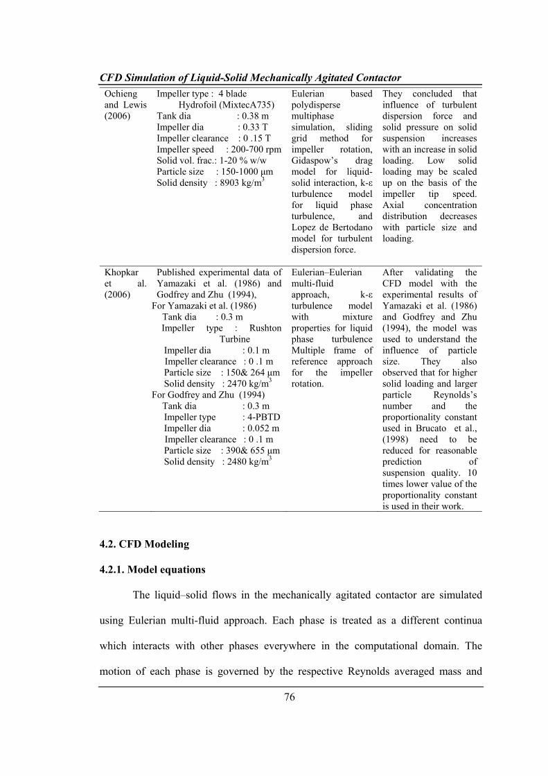
Ochieng and Lewis (2006)

Impeller type : 4 blade Hydrofoil (MixtecA735) Tank dia : 0.38 m Impeller dia : 0.33 T Impeller clearance : 0 .15 T Impeller speed : 200-700 rpm Solid vol. frac.: 1-20 % w/w Particle size : 150-1000 μm Solid density : 8903 kg/m3

Eulerian based polydisperse multiphase simulation, sliding grid method for impeller rotation, Gidaspow’s drag model for liquid-solid interaction, k-ε turbulence model for liquid phase turbulence, and Lopez de Bertodano model for turbulent dispersion force.

They concluded that influence of turbulent dispersion force and solid pressure on solid suspension increases with an increase in solid loading. Low solid loading may be scaled up on the basis of the impeller tip speed. Axial concentration distribution decreases with particle size and loading.

Khopkar et al. (2006)

Published experimental data of Yamazaki et al. (1986) and Godfrey and Zhu (1994),

For Yamazaki et al. (1986) Tank dia : 0.3 m

Impeller type : Rushton Turbine

Impeller dia : 0.1 m Impeller clearance : 0 .1 m

Particle size : 150& 264 μm Solid density : 2470 kg/m3

For Godfrey and Zhu (1994) Tank dia : 0.3 m

Impeller type : 4-PBTD Impeller dia : 0.052 m

Impeller clearance : 0 .1 m Particle size : 390& 655 μm Solid density : 2480 kg/m3

Eulerian–Eulerian multi-fluid approach, k-ε turbulence model with mixture properties for liquid phase turbulence Multiple frame of reference approach for the impeller rotation.

After validating the CFD model with the experimental results of Yamazaki et al. (1986) and Godfrey and Zhu (1994), the model was used to understand the influence of particle size. They also observed that for higher solid loading and larger particle Reynolds’s number and the proportionality constant used in Brucato et al., (1998) need to be reduced for reasonable prediction of suspension quality. 10 times lower value of the proportionality constant is used in their work.

4.2. CFD Modeling

4.2.1. Model equations

The liquid–solid flows in the mechanically agitated contactor are simulated

using Eulerian multi-fluid approach. Each phase is treated as a different continua

which interacts with other phases everywhere in the computational domain. The

motion of each phase is governed by the respective Reynolds averaged mass and


77

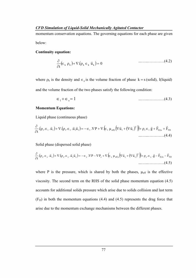
momentum conservation equations. The governing equations for each phase are given

below:

Continuity equation:

...…...…………(4.2)

where ρk is the density and k∈ is the volume fraction of phase l(liquid) (solid), sk =

and the volume fraction of the two phases satisfy the following condition:

...…...…………(4.3)

Momentum Equations:

Liquid phase (continuous phase)

...…...…………(4.4)

Solid phase (dispersed solid phase)

...…...…………(4.5)

where P is the pressure, which is shared by both the phases, μeff is the effective

viscosity. The second term on the RHS of the solid phase momentum equation (4.5)

accounts for additional solids pressure which arise due to solids collision and last term

(FD) in both the momentum equations (4.4) and (4.5) represents the drag force that

arise due to the momentum exchange mechanisms between the different phases.

( ) ( ) ( )( )( ) TDD,lsllT

lleff,llllllllll FFgρuuμ.P.uu..ρ.u..ρ.t

rrrrrrrr++∈+∇+∇∈∇+∇∈−=∈∇+∈

∂∂

( ) ( ) ( )( )( ) TDlsD,ssT

ssseff,ssssssssss FFg..ρuuμ.PP.uu..ρ.u..ρ.t

rrrrrrrr−−∈+∇+∇∈∇+∇−∇∈−=∈∇+∈

∂∂

( ) ( ) 0uρ.ρt kkkkk =∈∇+∈∂∂ r

1sl =∈+∈


78

4.2.2. Interphase momentum transfer

There are various interaction forces such as the drag force, the lift force and

the added mass force etc. during the momentum exchange between the different

phases. But the main interaction force is due to the drag force which is caused by the

slip between the different phases. Recently, Khopkar et al. (2003, 2005) studied the

influence of different interphase forces and reported that the effect of the virtual mass

force is not significant in the bulk region of agitated reactors and the magnitude of the

Basset force is also much smaller than that of the interphase drag force. Further they

also reported that the turbulent dispersion terms are significant only in the impeller

discharge stream. Very little influence of the virtual mass and lift force on the

simulated solid holdup profiles was also reported by Ljungqvist and Rasmuson

(2001). Hence based on their recommendations and also to reduce the computational

time, only the interphase drag force is considered in this work. In our CFD simulation,

the solid phase is treated as a dispersed phase and the liquid phase is treated as

continuous. Hence the drag force exerted by the dispersed phase on the continuous

phase is calculated as follows:

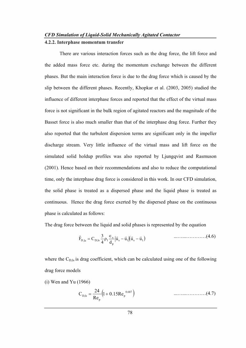
The drag force between the liquid and solid phases is represented by the equation

...…...…………(4.6)

where the CD,ls is drag coefficient, which can be calculated using one of the following

drag force models

(i) Wen and Yu (1966)

...…...…………(4.7)

( )lslsp

sllsD,ls,D uuuu

dρ

43CF rrrrr

−−∈

=

( )0.687p

plsD, 0.15Re1

Re24C +=


79

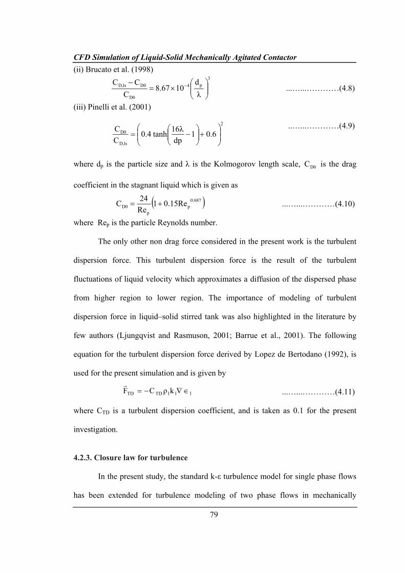
(ii) Brucato et al. (1998)

...…...…………(4.8)

(iii) Pinelli et al. (2001)

..…...…………(4.9)

where dp is the particle size and λ is the Kolmogorov length scale, D0C is the drag

coefficient in the stagnant liquid which is given as

...…...…………(4.10)

where Rep is the particle Reynolds number.

The only other non drag force considered in the present work is the turbulent

dispersion force. This turbulent dispersion force is the result of the turbulent

fluctuations of liquid velocity which approximates a diffusion of the dispersed phase

from higher region to lower region. The importance of modeling of turbulent

dispersion force in liquid–solid stirred tank was also highlighted in the literature by

few authors (Ljungqvist and Rasmuson, 2001; Barrue et al., 2001). The following

equation for the turbulent dispersion force derived by Lopez de Bertodano (1992), is

used for the present simulation and is given by

...…...…………(4.11)

where CTD is a turbulent dispersion coefficient, and is taken as 0.1 for the present

investigation.

4.2.3. Closure law for turbulence In the present study, the standard k-ε turbulence model for single phase flows

has been extended for turbulence modeling of two phase flows in mechanically

3p4

D0

D0D,ls

λd

108.67C

CC⎟⎟⎠

⎞⎜⎜⎝

⎛×=

− −

lllTDTD kρCF ∈∇−=r

2

lsD,

D0 0.61dp

16λ tanh0.4CC

⎟⎟⎠

⎞⎜⎜⎝

⎛+⎟⎟

⎠

⎞⎜⎜⎝

⎛−=

( )0.687p

pD0 0.15Re1

Re24C +=


80

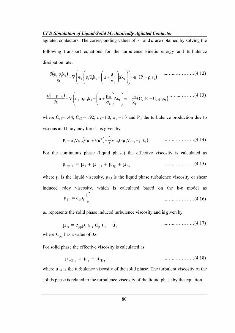
agitated contactors. The corresponding values of ε andk are obtained by solving the

following transport equations for the turbulence kinetic energy and turbulence

dissipation rate.

...…...…………(4.12)

.…....………(4.13)

where Cε1=1.44, Cε2 =1.92, σk=1.0, σε =1.3 and Pl, the turbulence production due to

viscous and buoyancy forces, is given by

...…...…………(4.14)

For the continuous phase (liquid phase) the effective viscosity is calculated as

..…...…………(4.15)

where μl is the liquid viscosity, μT,l is the liquid phase turbulence viscosity or shear

induced eddy viscosity, which is calculated based on the k-ε model as

...…...…………(4.16)

μts represents the solid phase induced turbulence viscosity and is given by

...…...…………(4.17)

where μpC has a value of 0.6.

For solid phase the effective viscosity is calculated as

...…...…………(4.18)

where μT,s is the turbulence viscosity of the solid phase. The turbulent viscosity of the

solids phase is related to the turbulence viscosity of the liquid phase by the equation

sT,sseff, μμμ +=

tstglT,lleff, μμμμμ +++=

εkρcμ

2

lμlT, =

lspslμpts uudρcμ rr−∈=

( ) ( )lllllk

tlllll

lll ερPΔkσμμkuρ.

tkρ

−=∈⎟⎟⎠

⎞⎜⎜⎝

⎛⎟⎟⎠

⎞⎜⎜⎝

⎛⎟⎟⎠

⎞⎜⎜⎝

⎛+−∈∇+

∂∈∂ r

( ) ( )llε2lε1l

lll

ε

tlllll

lll ερCPCkεΔε

σμμkuρ.

tερ

−=∈⎟⎟⎠

⎞⎜⎜⎝

⎛⎟⎟⎠

⎞⎜⎜⎝

⎛+−∈∇+

∂∈∂ r

( ) ( )llltllTllltll kρu.3μu.

32uu.uμP +∇∇−∇+∇∇=

rrrrr


81

...…...…………(4.19)

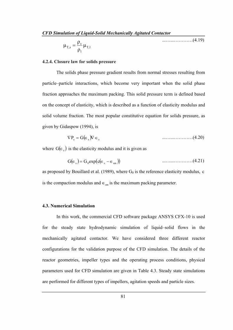
4.2.4. Closure law for solids pressure

The solids phase pressure gradient results from normal stresses resulting from

particle–particle interactions, which become very important when the solid phase

fraction approaches the maximum packing. This solid pressure term is defined based

on the concept of elasticity, which is described as a function of elasticity modulus and

solid volume fraction. The most popular constitutive equation for solids pressure, as

given by Gidaspow (1994), is

...…...…………(4.20)

where ( )sG ∈ is the elasticity modulus and it is given as

...…...…………(4.21)

as proposed by Bouillard et al. (1989), where G0 is the reference elasticity modulus, c

is the compaction modulus and sm∈ is the maximum packing parameter.

4.3. Numerical Simulation

In this work, the commercial CFD software package ANSYS CFX-10 is used

for the steady state hydrodynamic simulation of liquid–solid flows in the

mechanically agitated contactor. We have considered three different reactor

configurations for the validation purpose of the CFD simulation. The details of the

reactor geometries, impeller types and the operating process conditions, physical

parameters used for CFD simulation are given in Table 4.3. Steady state simulations

are performed for different types of impellers, agitation speeds and particle sizes.

lT,l

ssT, μ

ρρμ =

( ) ( )( )sms0s cexpGG ∈−∈=∈

( ) sss GP ∈∇∈=∇


82

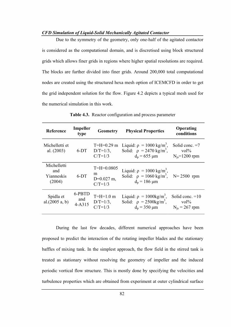
Due to the symmetry of the geometry, only one-half of the agitated contactor

is considered as the computational domain, and is discretised using block structured

grids which allows finer grids in regions where higher spatial resolutions are required.

The blocks are further divided into finer grids. Around 200,000 total computational

nodes are created using the structured hexa mesh option of ICEMCFD in order to get

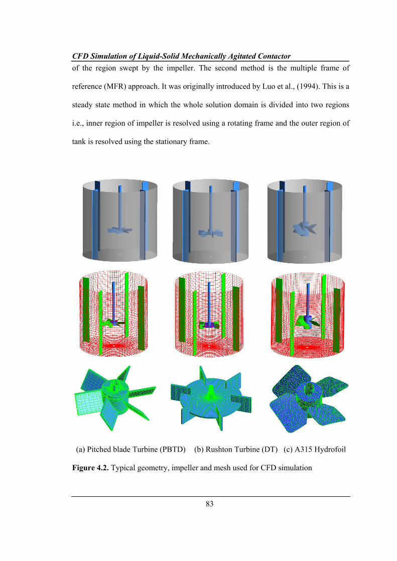
the grid independent solution for the flow. Figure 4.2 depicts a typical mesh used for

the numerical simulation in this work.

Table 4.3. Reactor configuration and process parameter

Reference Impeller type Geometry Physical Properties Operating

conditions

Michelletti et al. (2003)

6-DT

T=H=0.29 m D/T=1/3, C/T=1/3

Liquid: ρ = 1000 kg/m3, Solid: ρ = 2470 kg/m3, dp = 655 μm

Solid conc. =7 vol%

Njs=1200 rpm

Michelletti and

Yianneskis (2004)

6-DT

T=H=0.0805 m D=0.027 m, C/T=1/3

Liquid: ρ = 1000 kg/m3, Solid: ρ = 1060 kg/m3, dp = 186 μm

N= 2500 rpm

Spidla et al.(2005 a, b)

6-PBTD and

4-A315

T=H=1.0 m D/T=1/3, C/T=1/3

Liquid: ρ = 1000kg/m3, Solid: ρ = 2500kg/m3, dp = 350 μm

Solid conc. =10 vol%

Njs = 267 rpm

During the last few decades, different numerical approaches have been

proposed to predict the interaction of the rotating impeller blades and the stationary

baffles of mixing tank. In the simplest approach, the flow field in the stirred tank is

treated as stationary without resolving the geometry of impeller and the induced

periodic vortical flow structure. This is mostly done by specifying the velocities and

turbulence properties which are obtained from experiment at outer cylindrical surface


83

of the region swept by the impeller. The second method is the multiple frame of

reference (MFR) approach. It was originally introduced by Luo et al., (1994). This is a

steady state method in which the whole solution domain is divided into two regions

i.e., inner region of impeller is resolved using a rotating frame and the outer region of

tank is resolved using the stationary frame.

(a) Pitched blade Turbine (PBTD) (b) Rushton Turbine (DT) (c) A315 Hydrofoil

Figure 4.2. Typical geometry, impeller and mesh used for CFD simulation


84

The transformation of conservation equation into a rotating system yields

additional terms in the momentum equation namely the centrifugal and Coriolis force.

Another approach called inner-outer approach was introduced by Brucato et al.,

(1994). It is basically similar to the multiple frame of reference approach. The

difference between these two methods is that, there is a small overlap between the

calculation domain of the two regions and a large number of outer iterations are

required to ensure continuity across the interface between the two parts. The third

approach is the sliding grid approach. This method was first applied to the flow in a

stirred tank by Perng and Murthy (1993). In this approach, the inner region is rotated

during computation. The shape and the rotation of the impeller are therefore

represented exactly. Because the grid of the inner region is made to rotate and slide

along the interface with the outer region, this is fully transient and is considered as a

more accurate method, but it is also much more time consuming compared to MFR.

The final approach is the snapshot method. This was originally developed by Ranade

(1997). In this method the solution domain is divided into an inner region, in which

the time derivative term is approximated using a spatial derivative and in the outer

region, in which the time derivative term is neglected. The boundary between the

inner and outer region need to be selected in such a way that, the predicted results are

not sensitive to its actual location.

For the present simulation, we have used the MFR approach for simulating the

impeller rotation. In the MFR approach, the computational domain is divided into an

impeller zone (rotating reference frame) and a stationary zone (stationary reference

frame). The interaction of inner and outer regions is accounted by a suitable coupling


85

at the interface between the two regions where the continuity of the absolute velocity

is implemented. The boundary between the inner and the outer region is located at

r/R=0.6. No-slip boundary conditions are applied on the tank walls and shaft. The free

surface of tank is considered as the slip boundary condition. Initially the solid

particles are distributed in a homogeneous way inside the whole computational

domain. The discrete algebraic governing equations are obtained by the element based

finite volume method. The second order equivalent to high-resolution discretisation

scheme is applied for obtaining algebraic equations for momentum, volume fraction

of individual phases, turbulent kinetic energy and turbulence dissipation rate.

Pressure–velocity coupling was achieved by the Rhie-chow algorithm (1982).

The governing equations are solved using the advanced coupled multi grid

solver technology of ANSYS CFX-10. The criteria for convergence is set as 1 × 10−4

for the RMS residual error for all the governing equations. The RMS (Root Mean

Square) residual is obtained by taking all of the residuals throughout the domain,

squaring them, taking the mean, and then taking the square root of the mean for each

equation.

4.4. Results and Discussion

4.4.1. Single phase flow

Initially only the liquid flow (single phase) simulation of mechanically

agitated contactor was carried out to obtain the liquid phase flow field and this was

validated with the experimental data of Michelletti and Yianneskis (2004). They

carried out the measurements in a cylindrical vessel of diameter T = 0.0805 m and


86

height equal to the tank diameter. A six bladed Ruston Turbine of diameter D=T/3

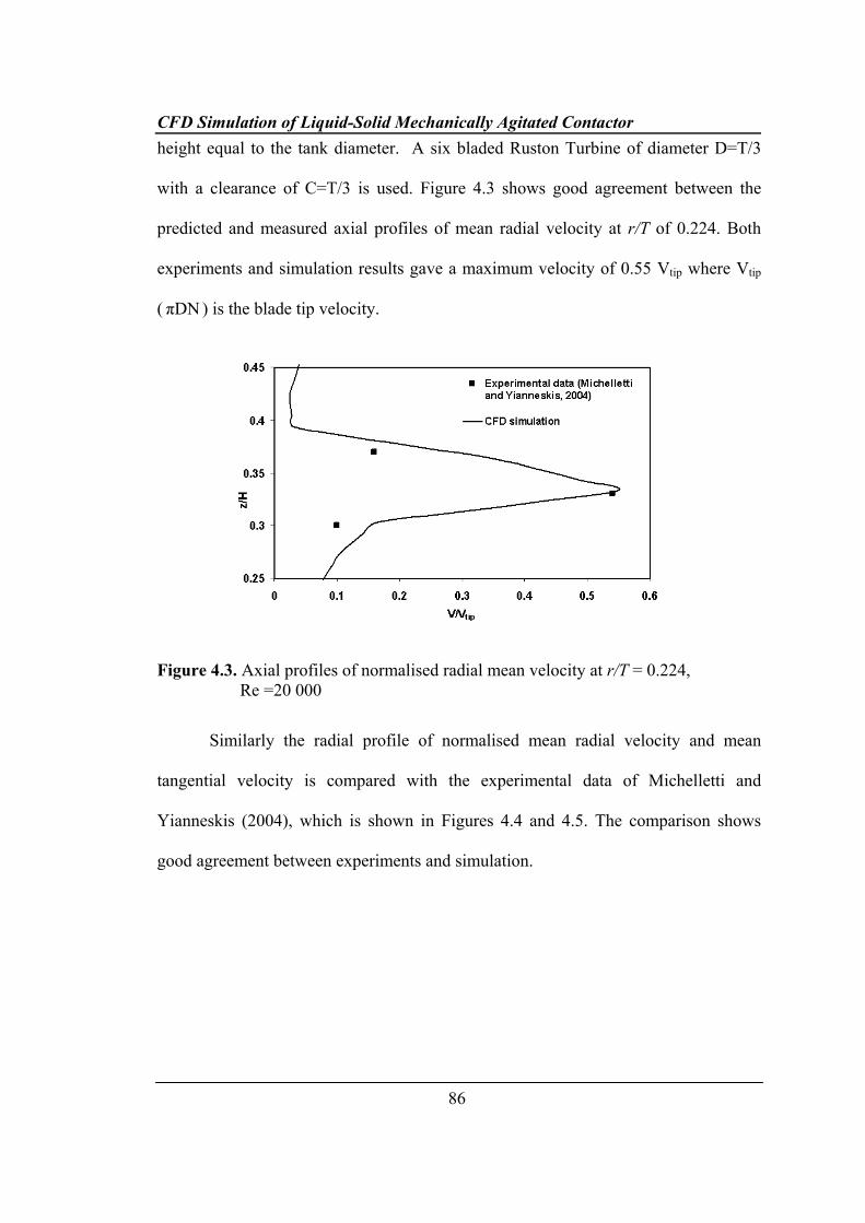
with a clearance of C=T/3 is used. Figure 4.3 shows good agreement between the

predicted and measured axial profiles of mean radial velocity at r/T of 0.224. Both

experiments and simulation results gave a maximum velocity of 0.55 Vtip where Vtip

( πDN ) is the blade tip velocity.

Figure 4.3. Axial profiles of normalised radial mean velocity at r/T = 0.224, Re =20 000

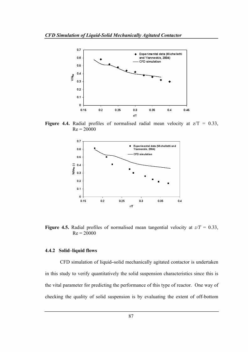
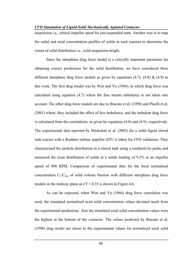
Similarly the radial profile of normalised mean radial velocity and mean

tangential velocity is compared with the experimental data of Michelletti and

Yianneskis (2004), which is shown in Figures 4.4 and 4.5. The comparison shows

good agreement between experiments and simulation.


87

Figure 4.4. Radial profiles of normalised radial mean velocity at z/T = 0.33, Re = 20000

Figure 4.5. Radial profiles of normalised mean tangential velocity at z/T = 0.33, Re = 20000

4.4.2 Solid–liquid flows

CFD simulation of liquid–solid mechanically agitated contactor is undertaken

in this study to verify quantitatively the solid suspension characteristics since this is

the vital parameter for predicting the performance of this type of reactor. One way of

checking the quality of solid suspension is by evaluating the extent of off-bottom


88

suspension i.e., critical impeller speed for just suspended state. Another way is to map

the radial and axial concentration profiles of solids in such reactors to determine the

extent of solid distribution i.e., solid suspension height.

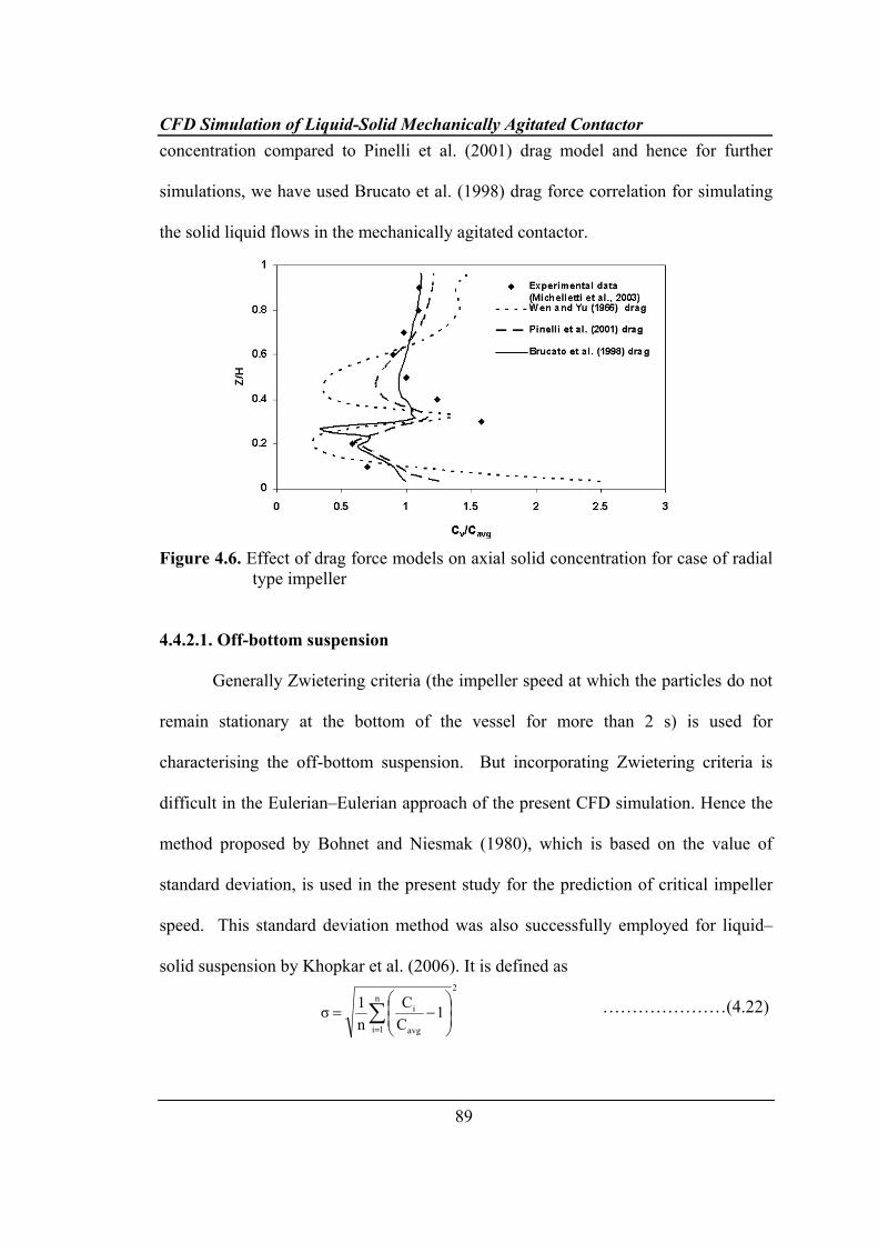
Since the interphase drag force model is a critically important parameter for

obtaining correct predictions for the solid distribution, we have considered three

different interphase drag force models as given by equations (4.7), (4.8) & (4.9) in

this work. The first drag model was by Wen and Yu (1966), in which drag force was

calculated using equation (4.7) where the free stream turbulence is not taken into

account. The other drag force models are due to Brucato et al. (1998) and Pinelli et al.

(2001) where, they included the effect of free turbulence, and the turbulent drag force

is calculated from the correlations, as given by equations (4.8) and (4.9), respectively.

The experimental data reported by Micheletti et al. (2003) for a solid–liquid stirred

tank reactor with a Rushton turbine impeller (DT) is taken for CFD validation. They

characterised the particle distribution in a stirred tank using a conductivity probe and

measured the axial distribution of solids at a solids loading of 9.2% at an impeller

speed of 988 RPM. Comparison of experimental data for the local normalised

concentration Cv/Cavg of solid volume fraction with different interphase drag force

models in the midway plane at r/T = 0.35 is shown in Figure 4.6.

As can be expected, when Wen and Yu (1966) drag force correlation was

used, the simulated normalised axial solid concentration values deviated much from

the experimental predictions. Also the simulated axial solid concentration values were

the highest at the bottom of the contactor. The values predicted by Brucato et al.

(1998) drag model are closer to the experimental values for normalized axial solid


89

concentration compared to Pinelli et al. (2001) drag model and hence for further

simulations, we have used Brucato et al. (1998) drag force correlation for simulating

the solid liquid flows in the mechanically agitated contactor.

Figure 4.6. Effect of drag force models on axial solid concentration for case of radial type impeller

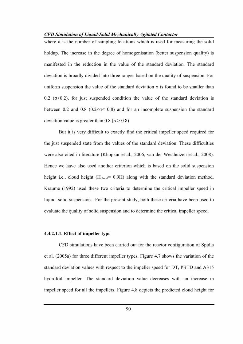
4.4.2.1. Off-bottom suspension

Generally Zwietering criteria (the impeller speed at which the particles do not

remain stationary at the bottom of the vessel for more than 2 s) is used for

characterising the off-bottom suspension. But incorporating Zwietering criteria is

difficult in the Eulerian–Eulerian approach of the present CFD simulation. Hence the

method proposed by Bohnet and Niesmak (1980), which is based on the value of

standard deviation, is used in the present study for the prediction of critical impeller

speed. This standard deviation method was also successfully employed for liquid–

solid suspension by Khopkar et al. (2006). It is defined as

…………………(4.22) 2

n

1i avg

i 1CC

n1σ ∑

=⎟⎟⎠

⎞⎜⎜⎝

⎛−=


90

where n is the number of sampling locations which is used for measuring the solid

holdup. The increase in the degree of homogenisation (better suspension quality) is

manifested in the reduction in the value of the standard deviation. The standard

deviation is broadly divided into three ranges based on the quality of suspension. For

uniform suspension the value of the standard deviation σ is found to be smaller than

0.2 (σ<0.2), for just suspended condition the value of the standard deviation is

between 0.2 and 0.8 (0.2<σ< 0.8) and for an incomplete suspension the standard

deviation value is greater than 0.8 (σ > 0.8).

But it is very difficult to exactly find the critical impeller speed required for

the just suspended state from the values of the standard deviation. These difficulties

were also cited in literature (Khopkar et al., 2006, van der Westhuizen et al., 2008).

Hence we have also used another criterion which is based on the solid suspension

height i.e., cloud height (Hcloud= 0.9H) along with the standard deviation method.

Kraume (1992) used these two criteria to determine the critical impeller speed in

liquid–solid suspension. For the present study, both these criteria have been used to

evaluate the quality of solid suspension and to determine the critical impeller speed.

4.4.2.1.1. Effect of impeller type

CFD simulations have been carried out for the reactor configuration of Spidla

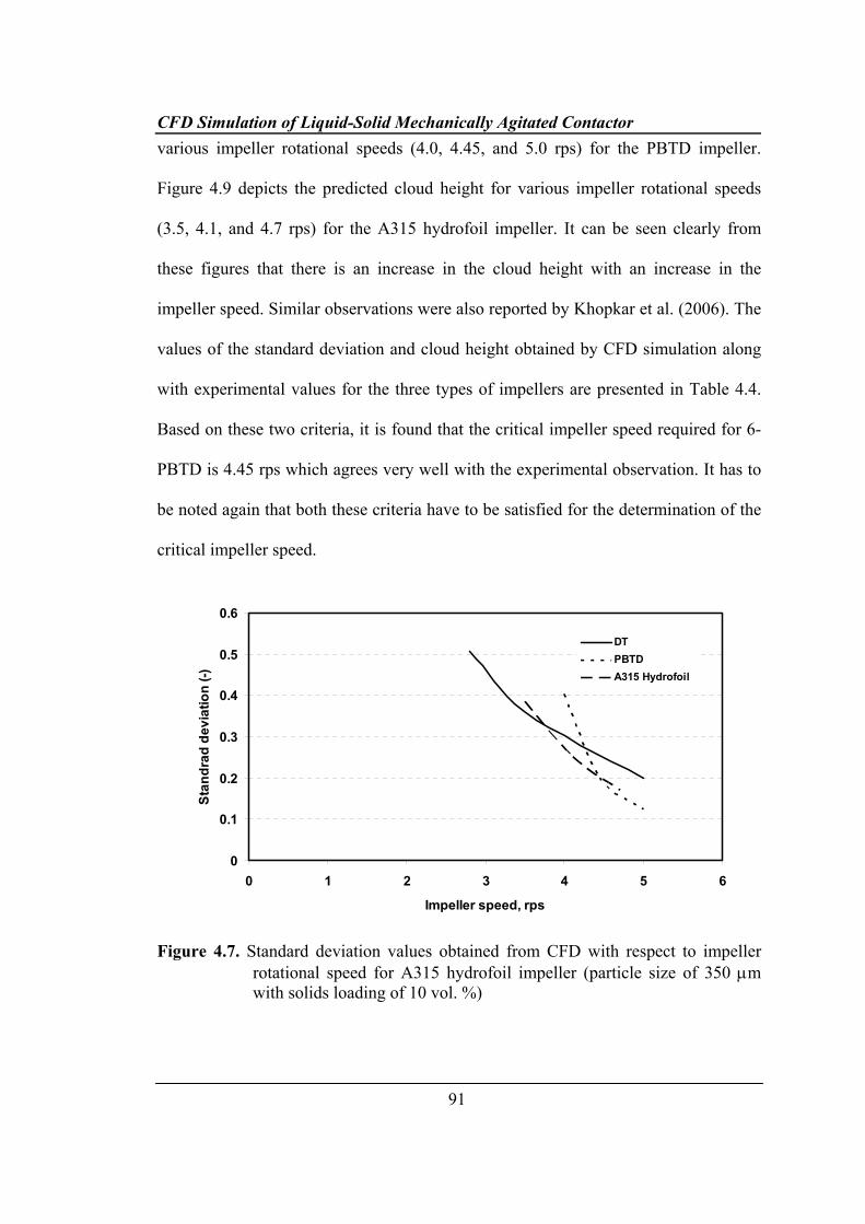
et al. (2005a) for three different impeller types. Figure 4.7 shows the variation of the

standard deviation values with respect to the impeller speed for DT, PBTD and A315

hydrofoil impeller. The standard deviation value decreases with an increase in

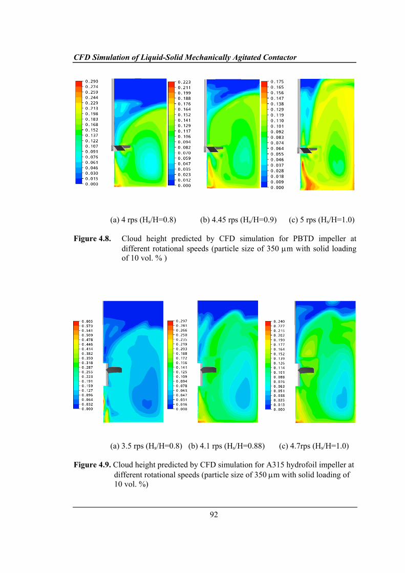
impeller speed for all the impellers. Figure 4.8 depicts the predicted cloud height for


91

various impeller rotational speeds (4.0, 4.45, and 5.0 rps) for the PBTD impeller.

Figure 4.9 depicts the predicted cloud height for various impeller rotational speeds

(3.5, 4.1, and 4.7 rps) for the A315 hydrofoil impeller. It can be seen clearly from

these figures that there is an increase in the cloud height with an increase in the

impeller speed. Similar observations were also reported by Khopkar et al. (2006). The

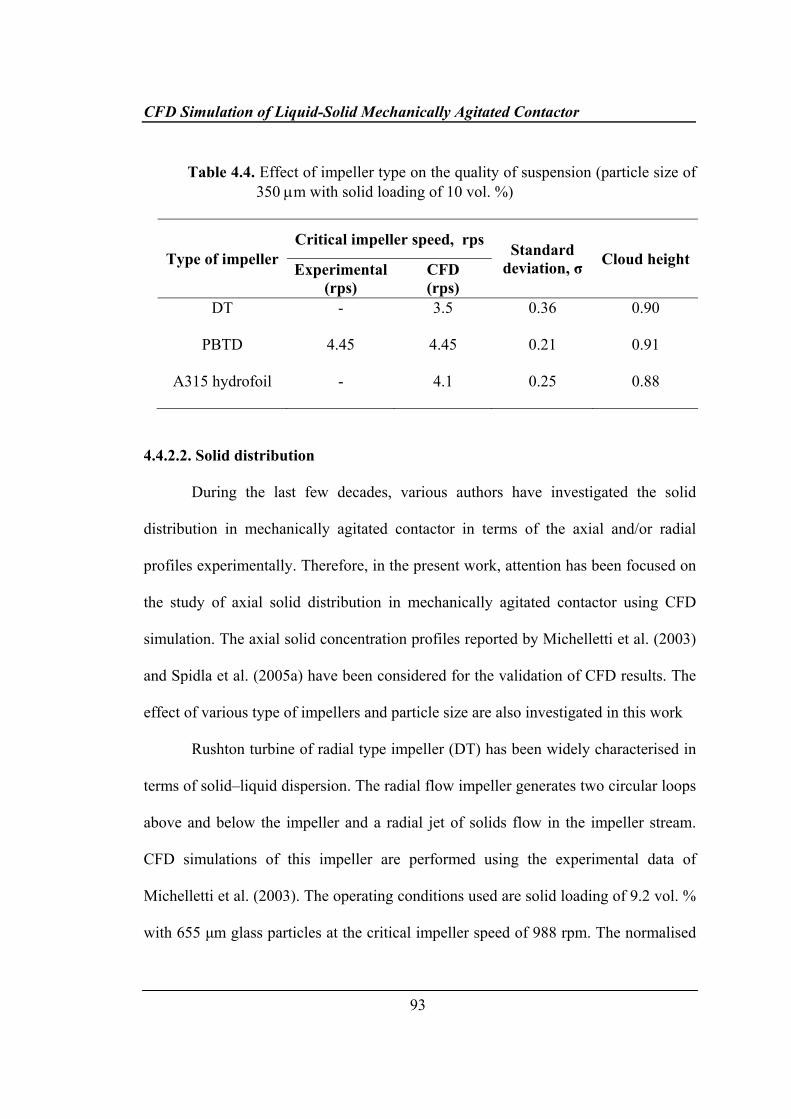
values of the standard deviation and cloud height obtained by CFD simulation along

with experimental values for the three types of impellers are presented in Table 4.4.

Based on these two criteria, it is found that the critical impeller speed required for 6-

PBTD is 4.45 rps which agrees very well with the experimental observation. It has to

be noted again that both these criteria have to be satisfied for the determination of the

critical impeller speed.

Figure 4.7. Standard deviation values obtained from CFD with respect to impeller rotational speed for A315 hydrofoil impeller (particle size of 350 μm with solids loading of 10 vol. %)

0

0.1

0.2

0.3

0.4

0.5

0.6

0 1 2 3 4 5 6

Impeller speed, rps

Stan

drad

dev

iatio

n (-)

DTPBTDA315 Hydrofoil


92

(a) 4 rps (Hs/H=0.8) (b) 4.45 rps (Hs/H=0.9) (c) 5 rps (Hs/H=1.0)

Figure 4.8. Cloud height predicted by CFD simulation for PBTD impeller at different rotational speeds (particle size of 350 μm with solid loading of 10 vol. % )

(a) 3.5 rps (Hs/H=0.8) (b) 4.1 rps (Hs/H=0.88) (c) 4.7rps (Hs/H=1.0)

Figure 4.9. Cloud height predicted by CFD simulation for A315 hydrofoil impeller at different rotational speeds (particle size of 350 μm with solid loading of 10 vol. %)


93

Table 4.4. Effect of impeller type on the quality of suspension (particle size of

350 μm with solid loading of 10 vol. %)

Type of impeller Critical impeller speed, rps Standard

deviation, σ Cloud height Experimental

(rps) CFD (rps)

DT - 3.5 0.36 0.90

PBTD 4.45 4.45 0.21 0.91

A315 hydrofoil - 4.1 0.25 0.88

4.4.2.2. Solid distribution

During the last few decades, various authors have investigated the solid

distribution in mechanically agitated contactor in terms of the axial and/or radial

profiles experimentally. Therefore, in the present work, attention has been focused on

the study of axial solid distribution in mechanically agitated contactor using CFD

simulation. The axial solid concentration profiles reported by Michelletti et al. (2003)

and Spidla et al. (2005a) have been considered for the validation of CFD results. The

effect of various type of impellers and particle size are also investigated in this work

Rushton turbine of radial type impeller (DT) has been widely characterised in

terms of solid–liquid dispersion. The radial flow impeller generates two circular loops

above and below the impeller and a radial jet of solids flow in the impeller stream.

CFD simulations of this impeller are performed using the experimental data of

Michelletti et al. (2003). The operating conditions used are solid loading of 9.2 vol. %

with 655 μm glass particles at the critical impeller speed of 988 rpm. The normalised


94

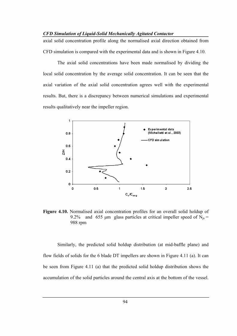
axial solid concentration profile along the normalised axial direction obtained from

CFD simulation is compared with the experimental data and is shown in Figure 4.10.

The axial solid concentrations have been made normalised by dividing the

local solid concentration by the average solid concentration. It can be seen that the

axial variation of the axial solid concentration agrees well with the experimental

results. But, there is a discrepancy between numerical simulations and experimental

results qualitatively near the impeller region.

Figure 4.10. Normalised axial concentration profiles for an overall solid holdup of

9.2% and 655 μm glass particles at critical impeller speed of Njs = 988 rpm

Similarly, the predicted solid holdup distribution (at mid-baffle plane) and

flow fields of solids for the 6 blade DT impellers are shown in Figure 4.11 (a). It can

be seen from Figure 4.11 (a) that the predicted solid holdup distribution shows the

accumulation of the solid particles around the central axis at the bottom of the vessel.


95

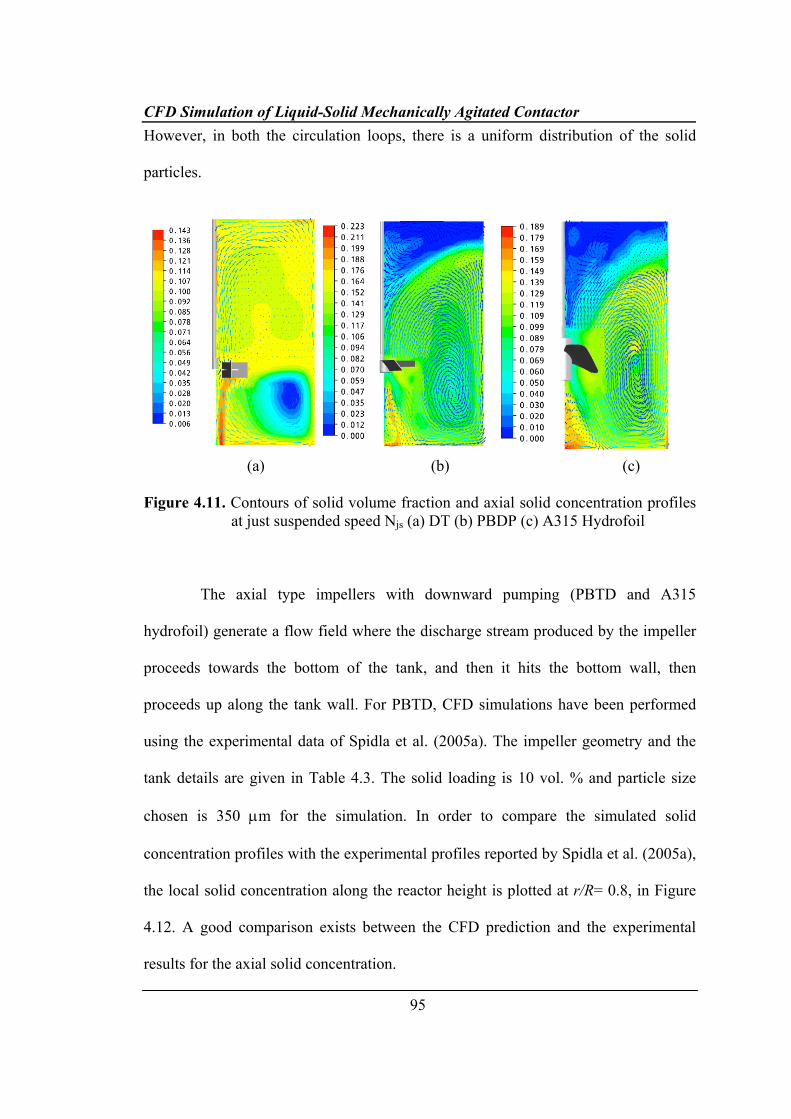
However, in both the circulation loops, there is a uniform distribution of the solid

particles.

(a) (b) (c) Figure 4.11. Contours of solid volume fraction and axial solid concentration profiles

at just suspended speed Njs (a) DT (b) PBDP (c) A315 Hydrofoil

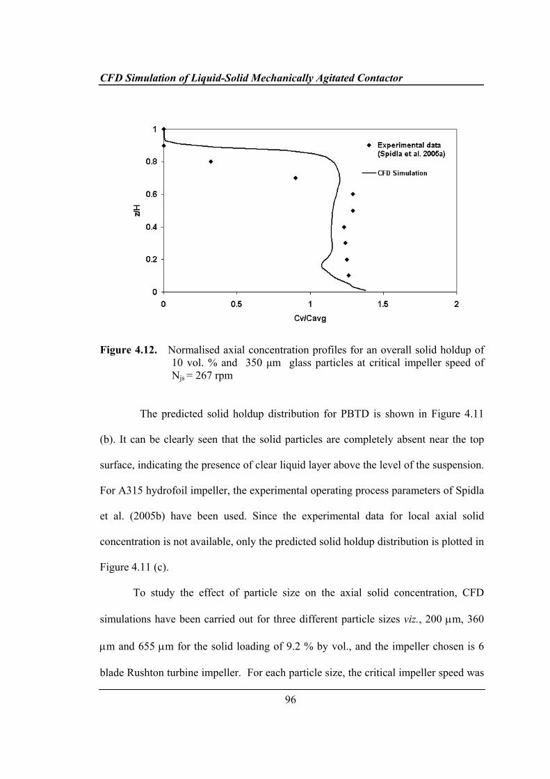
The axial type impellers with downward pumping (PBTD and A315

hydrofoil) generate a flow field where the discharge stream produced by the impeller

proceeds towards the bottom of the tank, and then it hits the bottom wall, then

proceeds up along the tank wall. For PBTD, CFD simulations have been performed

using the experimental data of Spidla et al. (2005a). The impeller geometry and the

tank details are given in Table 4.3. The solid loading is 10 vol. % and particle size

chosen is 350 μm for the simulation. In order to compare the simulated solid

concentration profiles with the experimental profiles reported by Spidla et al. (2005a),

the local solid concentration along the reactor height is plotted at r/R= 0.8, in Figure

4.12. A good comparison exists between the CFD prediction and the experimental

results for the axial solid concentration.


96

Figure 4.12. Normalised axial concentration profiles for an overall solid holdup of 10 vol. % and 350 μm glass particles at critical impeller speed of Njs = 267 rpm

The predicted solid holdup distribution for PBTD is shown in Figure 4.11

(b). It can be clearly seen that the solid particles are completely absent near the top

surface, indicating the presence of clear liquid layer above the level of the suspension.

For A315 hydrofoil impeller, the experimental operating process parameters of Spidla

et al. (2005b) have been used. Since the experimental data for local axial solid

concentration is not available, only the predicted solid holdup distribution is plotted in

Figure 4.11 (c).

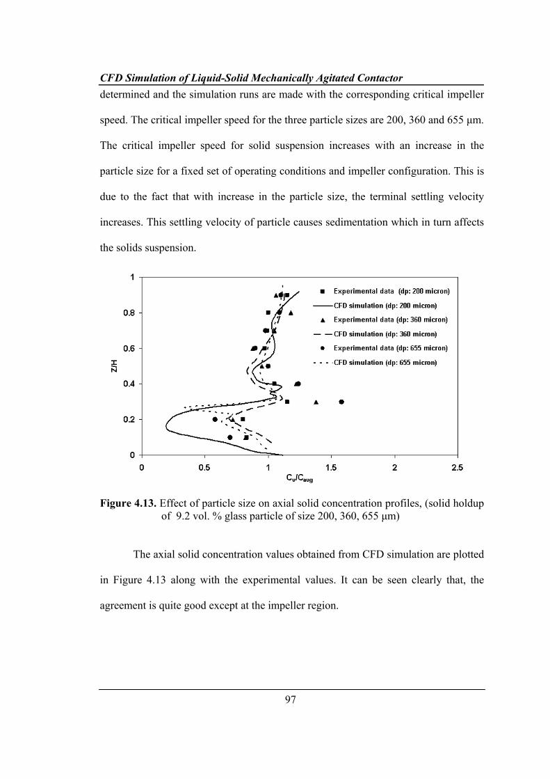
To study the effect of particle size on the axial solid concentration, CFD

simulations have been carried out for three different particle sizes viz., 200 μm, 360

μm and 655 μm for the solid loading of 9.2 % by vol., and the impeller chosen is 6

blade Rushton turbine impeller. For each particle size, the critical impeller speed was


97

determined and the simulation runs are made with the corresponding critical impeller

speed. The critical impeller speed for the three particle sizes are 200, 360 and 655 μm.

The critical impeller speed for solid suspension increases with an increase in the

particle size for a fixed set of operating conditions and impeller configuration. This is

due to the fact that with increase in the particle size, the terminal settling velocity

increases. This settling velocity of particle causes sedimentation which in turn affects

the solids suspension.

Figure 4.13. Effect of particle size on axial solid concentration profiles, (solid holdup

of 9.2 vol. % glass particle of size 200, 360, 655 μm)

The axial solid concentration values obtained from CFD simulation are plotted

in Figure 4.13 along with the experimental values. It can be seen clearly that, the

agreement is quite good except at the impeller region.


98

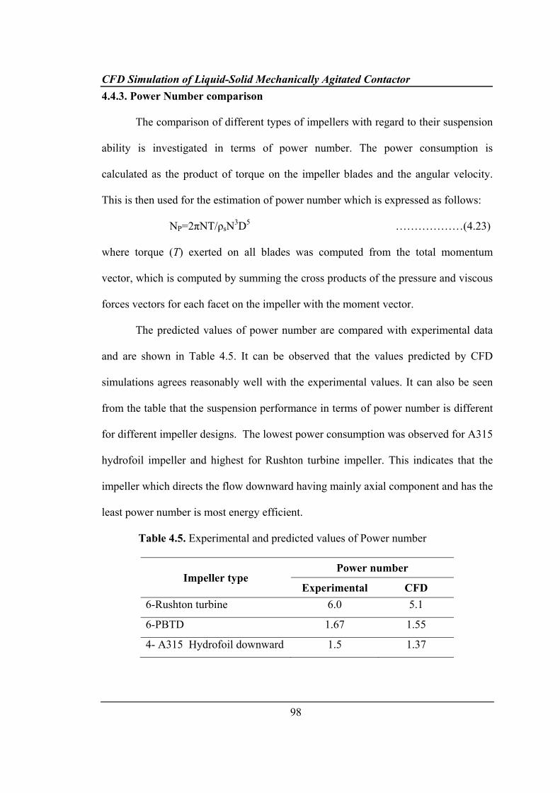
4.4.3. Power Number comparison

The comparison of different types of impellers with regard to their suspension

ability is investigated in terms of power number. The power consumption is

calculated as the product of torque on the impeller blades and the angular velocity.

This is then used for the estimation of power number which is expressed as follows:

NP=2πNT/ρsN3D5 ………………(4.23)

where torque (T) exerted on all blades was computed from the total momentum

vector, which is computed by summing the cross products of the pressure and viscous

forces vectors for each facet on the impeller with the moment vector.

The predicted values of power number are compared with experimental data

and are shown in Table 4.5. It can be observed that the values predicted by CFD

simulations agrees reasonably well with the experimental values. It can also be seen

from the table that the suspension performance in terms of power number is different

for different impeller designs. The lowest power consumption was observed for A315

hydrofoil impeller and highest for Rushton turbine impeller. This indicates that the

impeller which directs the flow downward having mainly axial component and has the

least power number is most energy efficient.

Table 4.5. Experimental and predicted values of Power number

Impeller type Power number

Experimental CFD 6-Rushton turbine 6.0 5.1

6-PBTD 1.67 1.55

4- A315 Hydrofoil downward 1.5 1.37


99

4.5. Conclusions

1. In this chapter, Eulerian multi-fluid approach along with standard k-ε turbulence

model has been used to study the solid suspension in liquid–solid mechanically

agitated contactor.

2. The results obtained from CFD simulations are validated qualitatively with

literature experimental data (Michelletti et al., 2003; Michelletti and Yianneskis

2004, Spidla et al., 2005a) in terms of axial profiles of solid distribution in liquid–

solid stirred suspension. A good agreement was found between the CFD

prediction and experimental data.

3. CFD predictions are compared quantitatively with literature experimental data

(Spidla et al., 2005a) in the terms of critical impeller speed based on the criteria of

standard deviation method and cloud height in a mechanically agitated contactor.

An adequate agreement was found between CFD prediction and the experimental

data.

4. The numerical simulation has further been extended to study the effect of impeller

design (DT, PBTD and A315 Hydrofoil), impeller speed and particle size (200–

650 μm) on the solid suspension in liquid–solid mechanically agitated contactor.

CFD Simulation of Liquid-Solid Mechanically...

Documents

Transcript of CFD Simulation of Liquid-Solid Mechanically...