
CFD application for impact & risk assessment in the ... · SCAV C V C V εεεk ε ε =− = −...
39
CFD application for impact & risk assessment in the Industrial Areas-Case Studies Fluidyn-PANEPR for local scale short-term Claude Souprayen, Fluidyn France [email protected] EAN – ALARA Workshop Lisbonne 15-17 May 2017
-
Upload
truongkhanh -
Category
Documents
-
view
215 -
download
0
Transcript of CFD application for impact & risk assessment in the ... · SCAV C V C V εεεk ε ε =− = −...
CFD application for impact & risk assessment in the Industrial Areas-Case Studies
Fluidyn-PANEPR for local scale short-term
Claude Souprayen, Fluidyn France [email protected]
EAN – ALARA Workshop Lisbonne 15-17 May 2017
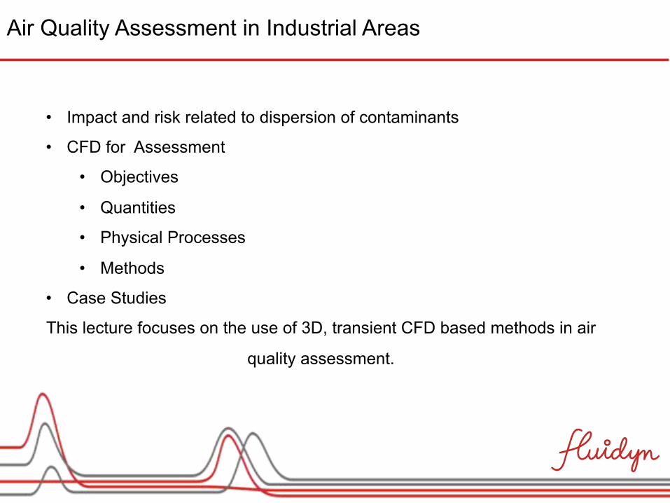
• Impact and risk related to dispersion of contaminants
• CFD for Assessment
• Objectives
• Quantities
• Physical Processes
• Methods
• Case Studies
This lecture focuses on the use of 3D, transient CFD based methods in air
quality assessment.
Air Quality Assessment in Industrial Areas
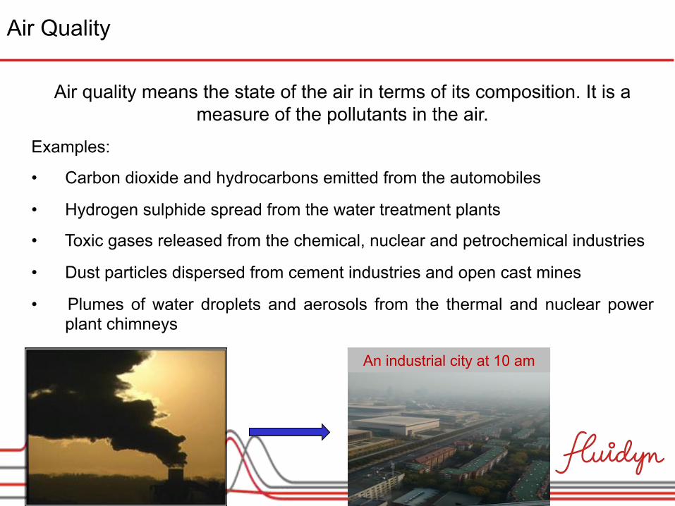
Air quality means the state of the air in terms of its composition. It is a measure of the pollutants in the air.
Examples:
• Carbon dioxide and hydrocarbons emitted from the automobiles
• Hydrogen sulphide spread from the water treatment plants
• Toxic gases released from the chemical, nuclear and petrochemical industries
• Dust particles dispersed from cement industries and open cast mines
• Plumes of water droplets and aerosols from the thermal and nuclear power plant chimneys
Air Quality
An industrial city at 10 am
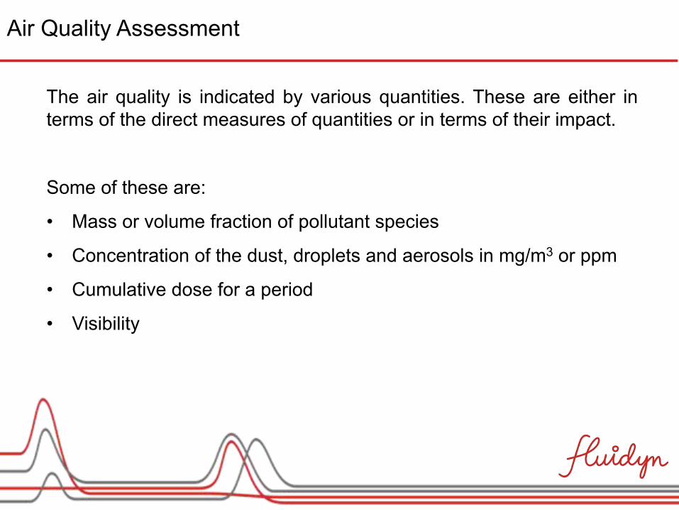
The air quality is indicated by various quantities. These are either in terms of the direct measures of quantities or in terms of their impact.
Some of these are:
• Mass or volume fraction of pollutant species
• Concentration of the dust, droplets and aerosols in mg/m3 or ppm
• Cumulative dose for a period
• Visibility
Air Quality Assessment
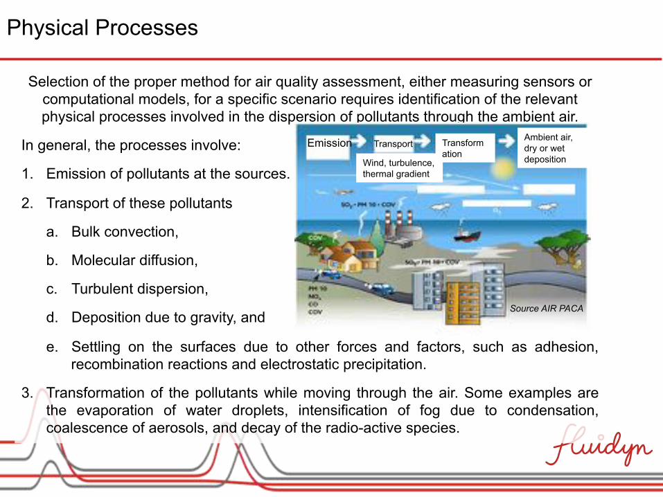
Selection of the proper method for air quality assessment, either measuring sensors or computational models, for a specific scenario requires identification of the relevant physical processes involved in the dispersion of pollutants through the ambient air.
In general, the processes involve:
1. Emission of pollutants at the sources.
2. Transport of these pollutants
a. Bulk convection,
b. Molecular diffusion,
c. Turbulent dispersion,
d. Deposition due to gravity, and
e. Settling on the surfaces due to other forces and factors, such as adhesion, recombination reactions and electrostatic precipitation.
3. Transformation of the pollutants while moving through the air. Some examples are the evaporation of water droplets, intensification of fog due to condensation, coalescence of aerosols, and decay of the radio-active species.
Physical Processes
Emission Transport
Wind, turbulence, thermal gradient
Transformation
Ambient air, dry or wet deposition
Source AIR PACA
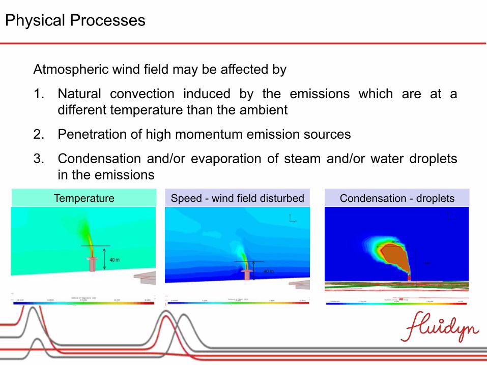
Atmospheric wind field may be affected by
1. Natural convection induced by the emissions which are at a different temperature than the ambient
2. Penetration of high momentum emission sources
3. Condensation and/or evaporation of steam and/or water droplets in the emissions
Physical Processes
Temperature Speed - wind field disturbed Condensation - droplets
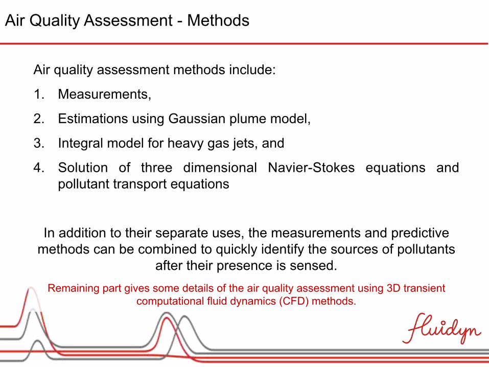
Air quality assessment methods include:
1. Measurements,
2. Estimations using Gaussian plume model,
3. Integral model for heavy gas jets, and
4. Solution of three dimensional Navier-Stokes equations and pollutant transport equations
In addition to their separate uses, the measurements and predictive methods can be combined to quickly identify the sources of pollutants
after their presence is sensed. Remaining part gives some details of the air quality assessment using 3D transient
computational fluid dynamics (CFD) methods.
Air Quality Assessment - Methods
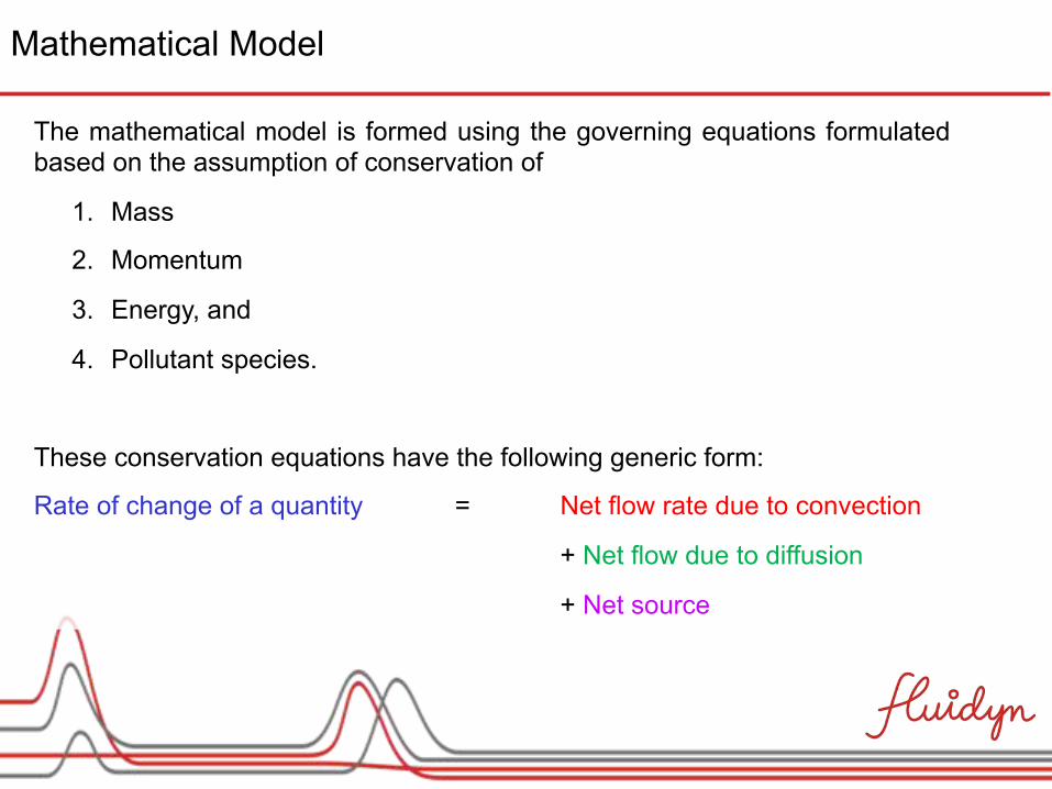
The mathematical model is formed using the governing equations formulated based on the assumption of conservation of
1. Mass
2. Momentum
3. Energy, and
4. Pollutant species.
These conservation equations have the following generic form:
Rate of change of a quantity = Net flow rate due to convection
+ Net flow due to diffusion
+ Net source
Mathematical Model
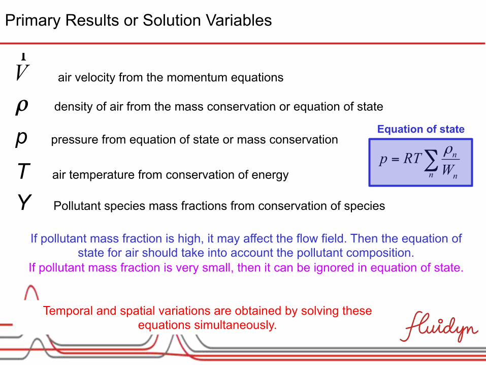
Primary Results or Solution Variables
Temporal and spatial variations are obtained by solving these equations simultaneously.
air velocity from the momentum equations
p pressure from equation of state or mass conservation
ρ density of air from the mass conservation or equation of state
Vr
T air temperature from conservation of energy
Y Pollutant species mass fractions from conservation of species
n
n n
p RTWρ
= ∑
Equation of state
If pollutant mass fraction is high, it may affect the flow field. Then the equation of state for air should take into account the pollutant composition.
If pollutant mass fraction is very small, then it can be ignored in equation of state.
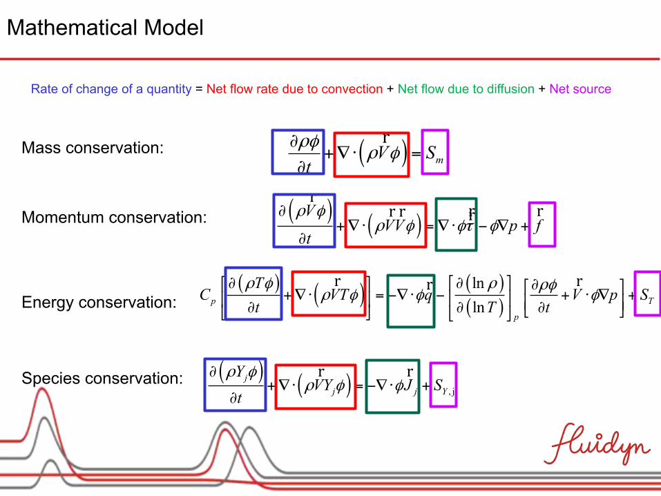
Mathematical Model
Mass conservation: ( ) mV Stρφ
ρ φ∂
+∇⋅ =∂
r
Momentum conservation: ( ) ( )V
VV p ft
ρ φρ φ φτ φ
∂+∇⋅ =∇⋅ − ∇ +
∂
rr rr r r
Energy conservation: ( ) ( ) ( )
( )lnlnp T
p
TC VT q V p S
t T tρ φ ρ ρφ
ρ φ φ φ# $∂ ∂# $ ∂# $+∇⋅ = −∇⋅ − + ⋅ ∇ +) *) * ) *∂ ∂ ∂+ ,+ , + ,
r rr
Species conservation: ( ) ( ) , jj
j j Y
YVY J S
tρ φ
ρ φ φ∂
+∇⋅ = −∇⋅ +∂
r r
Rate of change of a quantity = Net flow rate due to convection + Net flow due to diffusion + Net source
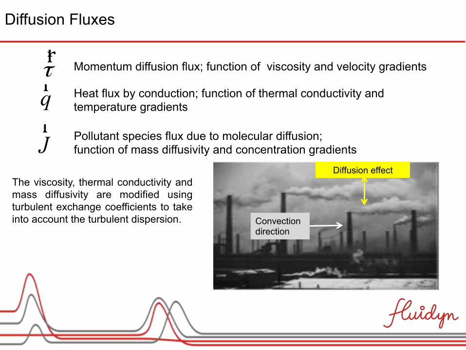
Diffusion Fluxes
Momentum diffusion flux; function of viscosity and velocity gradients
Heat flux by conduction; function of thermal conductivity and temperature gradients
τrrqr
Jr Pollutant species flux due to molecular diffusion;
function of mass diffusivity and concentration gradients
The viscosity, thermal conductivity and mass diffusivity are modified using turbulent exchange coefficients to take into account the turbulent dispersion. Convection
direction
Diffusion effect
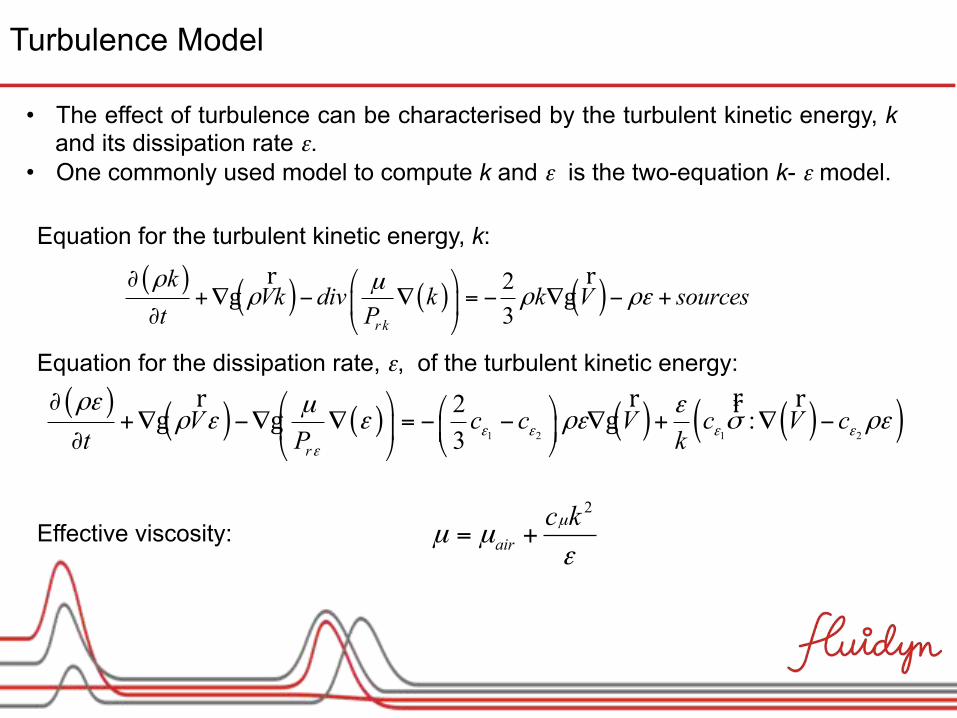
Turbulence Model
• The effect of turbulence can be characterised by the turbulent kinetic energy, k and its dissipation rate ε.
• One commonly used model to compute k and ε is the two-equation k- ε model.
Equation for the turbulent kinetic energy, k:
( ) ( ) ( ) ( )23rk
kVk div k k V sources
t Pρ µ
ρ ρ ρε∂ $ %
+∇ − ∇ = − ∇ − +( )∂ * +
r rg g
Equation for the dissipation rate, ε, of the turbulent kinetic energy:
( ) ( ) ( ) ( ) ( )( )1 2 1 2
2 :3r
V c c V c V ct P kε ε ε ε
ε
ρε µ ερ ε ε ρε σ ρε
∂ % & % &+∇ −∇ ∇ = − − ∇ + ∇ −) * ) *∂ + ,+ ,
rr r rrg g g
2
airc kµ
µ µε
= +Effective viscosity:
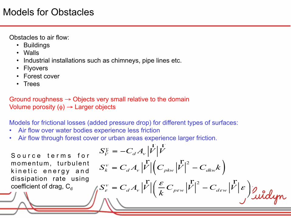
Models for Obstacles
Obstacles to air flow: • Buildings • Walls • Industrial installations such as chimneys, pipe lines etc. • Flyovers • Forest cover • Trees
Ground roughness → Objects very small relative to the domain Volume porosity (φ) → Larger objects Models for frictional losses (added pressure drop) for different types of surfaces: • Air flow over water bodies experience less friction • Air flow through forest cover or urban areas experience larger friction.
( )2
2
vd vV
vk d v pkw dkw
vd v p w d w
S C A V V
S C A V C V C k
S C A V C V C Vkε ε εε
ε
= −
= −
# $= −% &' (
rr r
r r
r r r
S o u r c e t e r m s f o r momentum, tu rbu len t k i n e t i c e n e r g y a n d dissipation rate using coefficient of drag, Cd
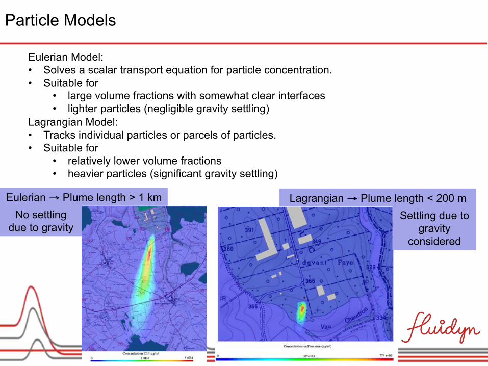
Particle Models
Eulerian Model: • Solves a scalar transport equation for particle concentration. • Suitable for
• large volume fractions with somewhat clear interfaces • lighter particles (negligible gravity settling)
Lagrangian Model: • Tracks individual particles or parcels of particles. • Suitable for
• relatively lower volume fractions • heavier particles (significant gravity settling)
Eulerian → Plume length > 1 km Lagrangian → Plume length < 200 m No settling
due to gravity Settling due to
gravity considered
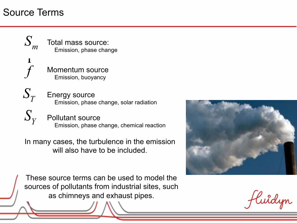
Source Terms
Momentum source Emission, buoyancy
Energy source Emission, phase change, solar radiation
fr
TS
YS Pollutant source Emission, phase change, chemical reaction
In many cases, the turbulence in the emission will also have to be included.
mS Total mass source: Emission, phase change
These source terms can be used to model the sources of pollutants from industrial sites, such
as chimneys and exhaust pipes.
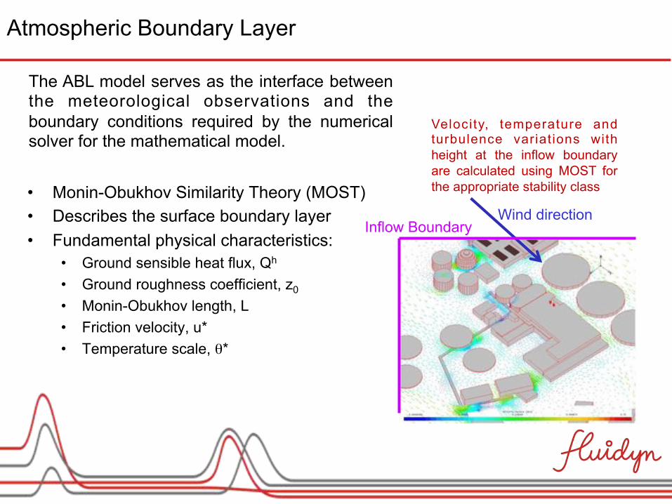
• Monin-Obukhov Similarity Theory (MOST) • Describes the surface boundary layer • Fundamental physical characteristics:
• Ground sensible heat flux, Qh
• Ground roughness coefficient, z0
• Monin-Obukhov length, L • Friction velocity, u* • Temperature scale, θ*
Atmospheric Boundary Layer
Wind direction
Velocity, temperature and turbulence variations with height at the inflow boundary are calculated using MOST for the appropriate stability class
Inflow Boundary
The ABL model serves as the interface between the meteorological observations and the boundary conditions required by the numerical solver for the mathematical model.
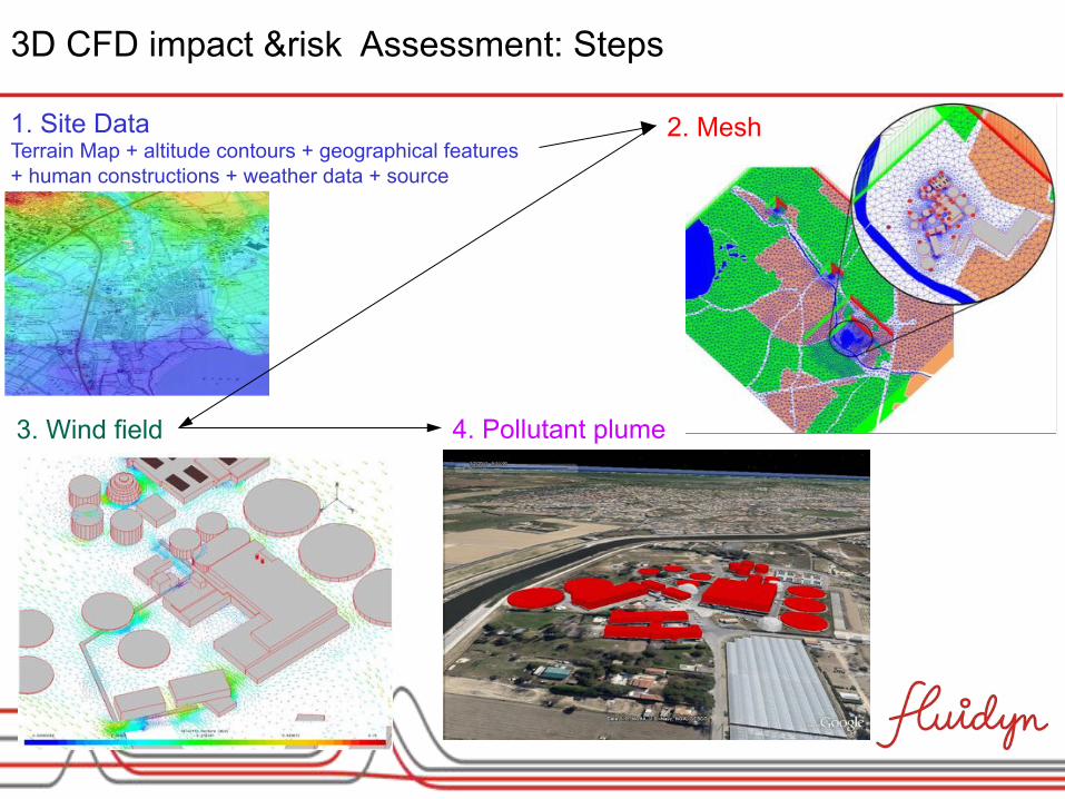
3D CFD impact &risk Assessment: Steps
1. Site Data Terrain Map + altitude contours + geographical features + human constructions + weather data + source
2. Mesh
3. Wind field 4. Pollutant plume
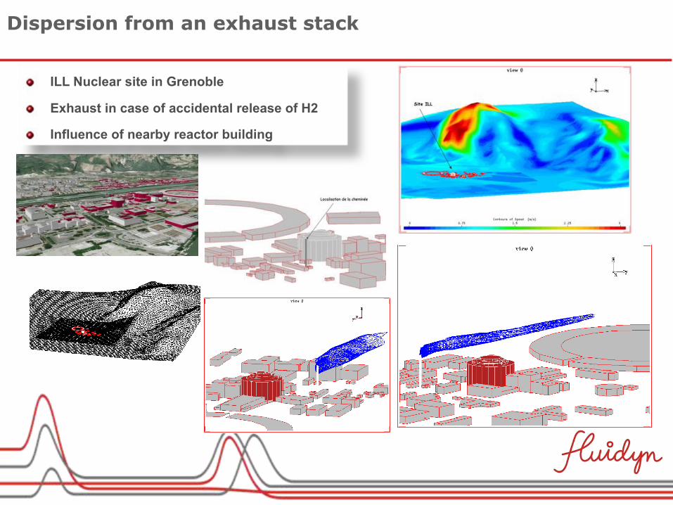
Dispersion from an exhaust stack
ILL Nuclear site in Grenoble
Exhaust in case of accidental release of H2
Influence of nearby reactor building
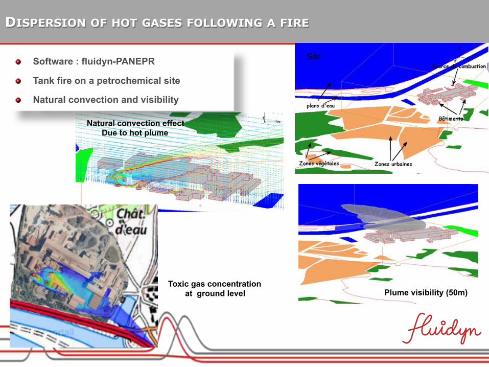
DISPERSION OF HOT GASES FOLLOWING A FIRE
Software : fluidyn-PANEPR
Tank fire on a petrochemical site
Natural convection and visibility
Site
Natural convection effect Due to hot plume
Plume visibility (50m) Toxic gas concentration
at ground level
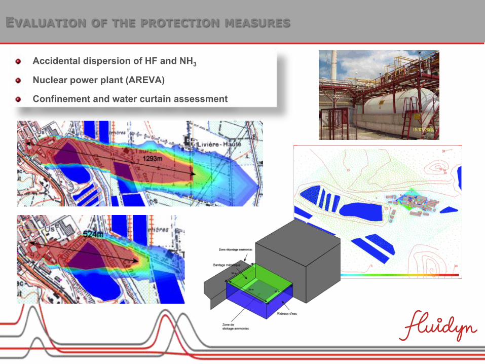
EVALUATION OF THE PROTECTION MEASURES
Accidental dispersion of HF and NH3
Nuclear power plant (AREVA)
Confinement and water curtain assessment
Site pétrochimique
• Aim: • Sense pollutant presence • Locate and quantify the pollutant source • Predict short term dispersion
• Uses weather and wind field predictions and real time data from monitor points.
• Calculate source strength, location, time and duration.
• Short term prediction is done using faster than real time CFD simulations. • This information helps to estimate the extent of dispersion of harmful
pollutants and helps in executing the mitigation measures.
Case Study 3: Real Time Monitoring and Warning
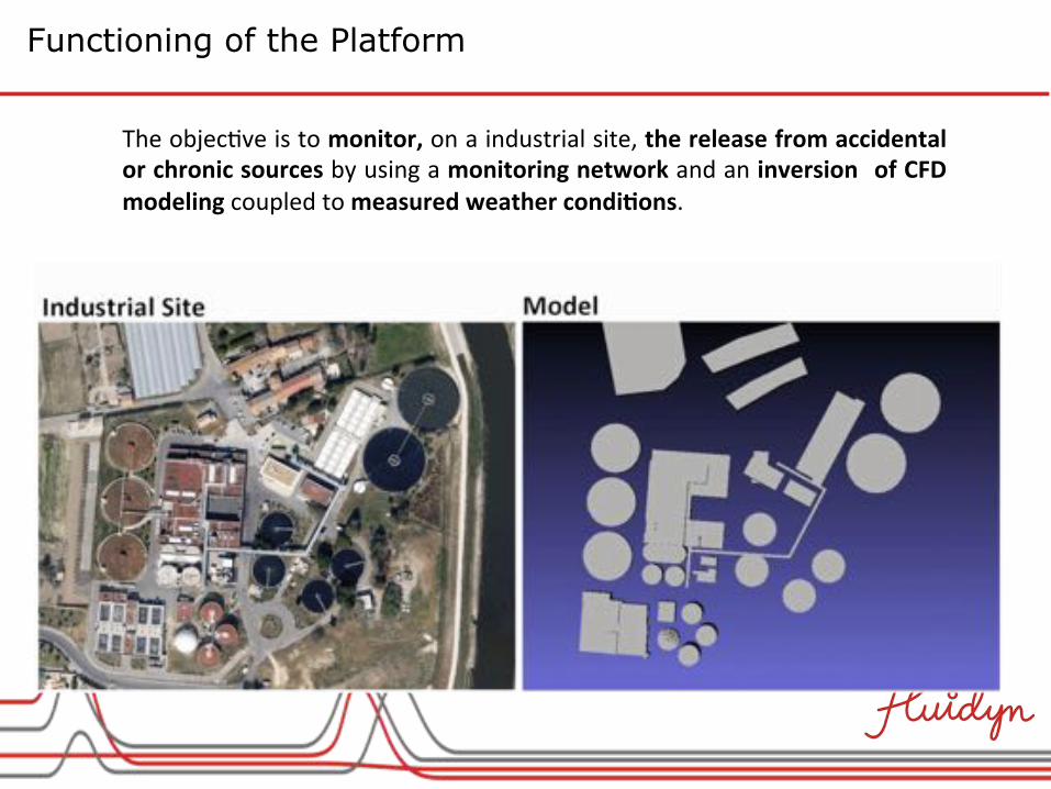
The$objec)ve$is$to$monitor,$on$a$industrial$site,$the*release*from*accidental*or*chronic*sources*by$using$a$monitoring*network*and$an$inversion* *of*CFD*modeling*coupled$to$measured*weather*condi9ons.$
Functioning of the Platform
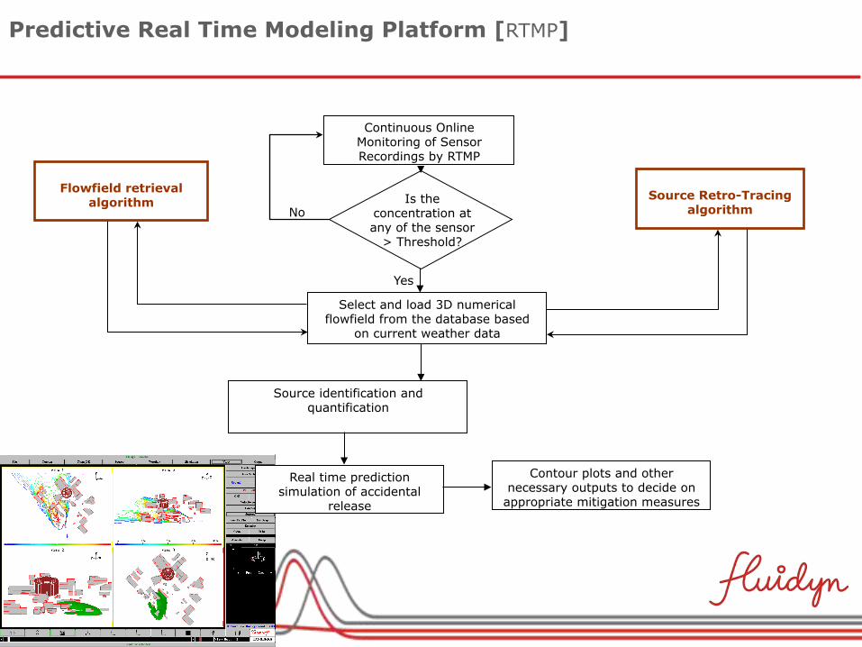
Select and load 3D numerical flowfield from the database based
on current weather data
Flowfield retrieval
algorithm
Source Retro-Tracing algorithm
Source identification and quantification
Real time prediction simulation of accidental
release Contour plots and other
necessary outputs to decide on appropriate mitigation measures
Continuous Online Monitoring of Sensor Recordings by RTMP
Is the concentration at any of the sensor
> Threshold? Yes
No
Predictive Real Time Modeling Platform [RTMP]
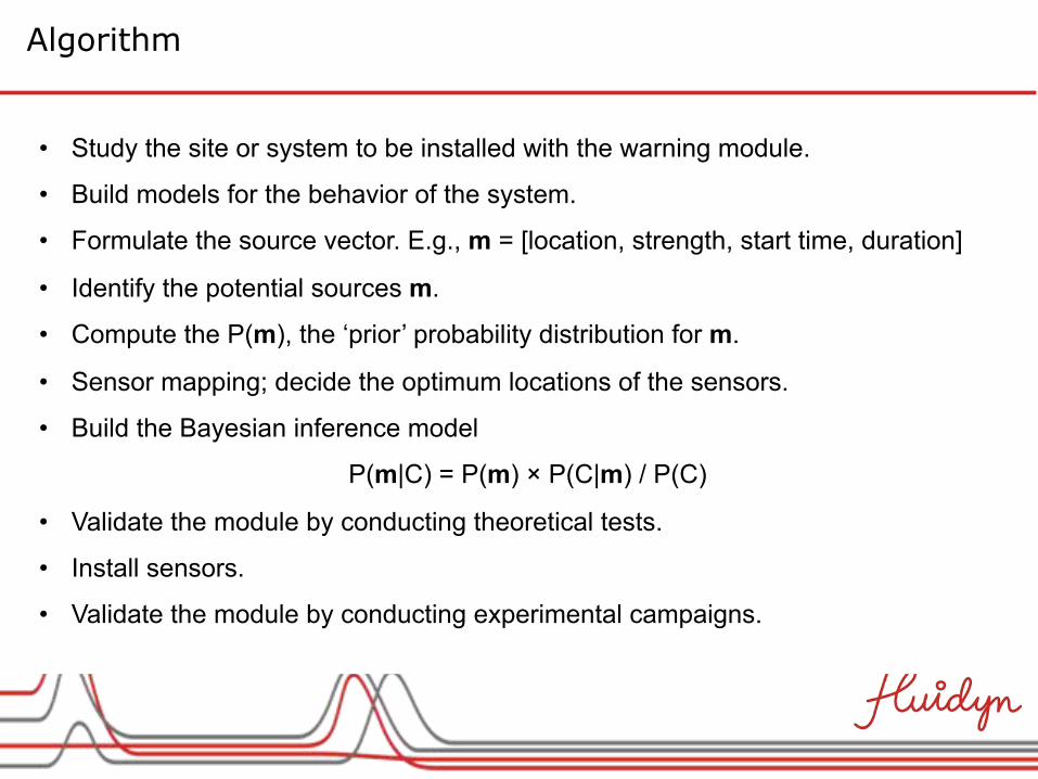
Algorithm
• Study the site or system to be installed with the warning module.
• Build models for the behavior of the system.
• Formulate the source vector. E.g., m = [location, strength, start time, duration]
• Identify the potential sources m.
• Compute the P(m), the ‘prior’ probability distribution for m.
• Sensor mapping; decide the optimum locations of the sensors.
• Build the Bayesian inference model
P(m|C) = P(m) × P(C|m) / P(C)
• Validate the module by conducting theoretical tests.
• Install sensors.
• Validate the module by conducting experimental campaigns.
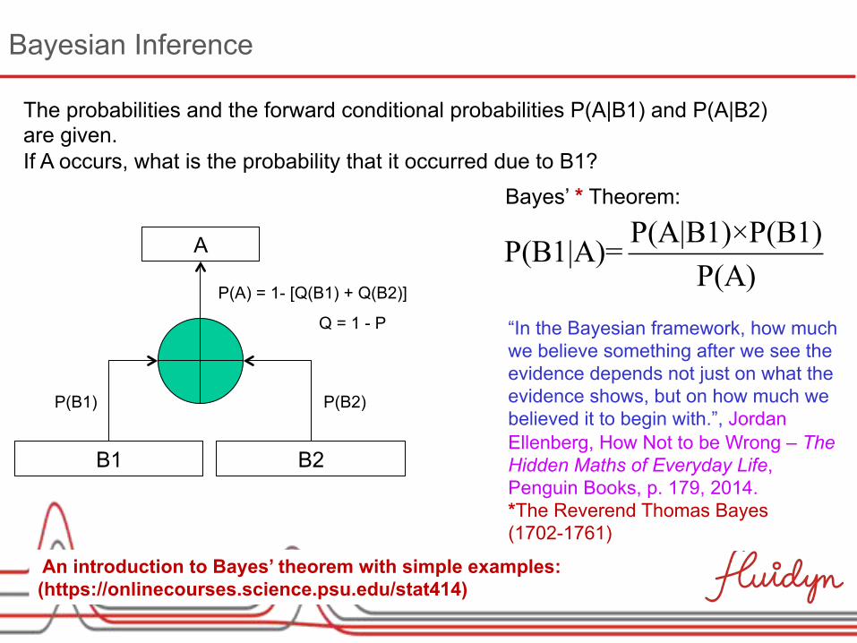
Bayesian Inference
A
B1 B2
P(B2) P(B1)
Q = 1 - P
P(A) = 1- [Q(B1) + Q(B2)]
The probabilities and the forward conditional probabilities P(A|B1) and P(A|B2) are given. If A occurs, what is the probability that it occurred due to B1?
Bayes’ * Theorem:
P(A|B1)×P(B1)P(B1|A)=P(A)
“In the Bayesian framework, how much we believe something after we see the evidence depends not just on what the evidence shows, but on how much we believed it to begin with.”, Jordan Ellenberg, How Not to be Wrong – The Hidden Maths of Everyday Life, Penguin Books, p. 179, 2014. *The Reverend Thomas Bayes (1702-1761)
An introduction to Bayes’ theorem with simple examples: (https://onlinecourses.science.psu.edu/stat414)
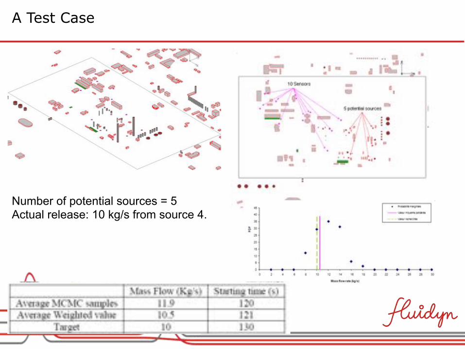
A Test Case
Number of potential sources = 5 Actual release: 10 kg/s from source 4.
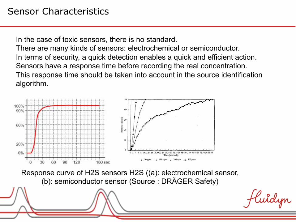
Sensor Characteristics
In the case of toxic sensors, there is no standard. There are many kinds of sensors: electrochemical or semiconductor. In terms of security, a quick detection enables a quick and efficient action. Sensors have a response time before recording the real concentration. This response time should be taken into account in the source identification algorithm.
Response curve of H2S sensors H2S ((a): electrochemical sensor, (b): semiconductor sensor (Source : DRÄGER Safety)
More details in …
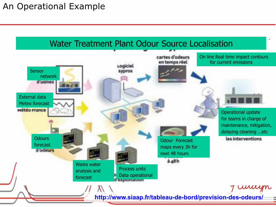
Water Treatment Plant Odour Source Localisation
Sensor network
External data Meteo forecast
Odours forecast
Waste water analysis and forecast
Process units Data operational
Odour Forecast maps every 3h for next 48 hours
On line Real time impact contours for current emissions
Operational update for teams in charge of maintenance, mitigation, delaying cleaning …etc
An Operational Example
http://www.siaap.fr/tableau-de-bord/prevision-des-odeurs/
http://www.siaap.fr/tableau-de-bord/prevision-des-odeurs/
13 February, 2016: 01:00 – 04:00 (LocalTime)
Working Example: Pollutant Prediction
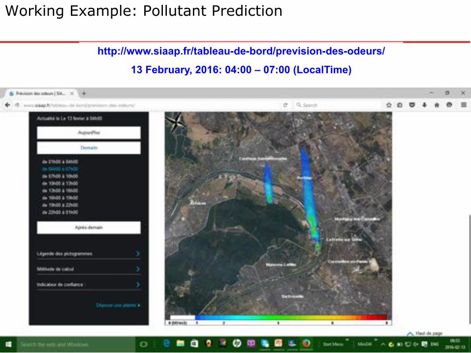
http://www.siaap.fr/tableau-de-bord/prevision-des-odeurs/
13 February, 2016: 04:00 – 07:00 (LocalTime)
Working Example: Pollutant Prediction
http://www.siaap.fr/tableau-de-bord/prevision-des-odeurs/
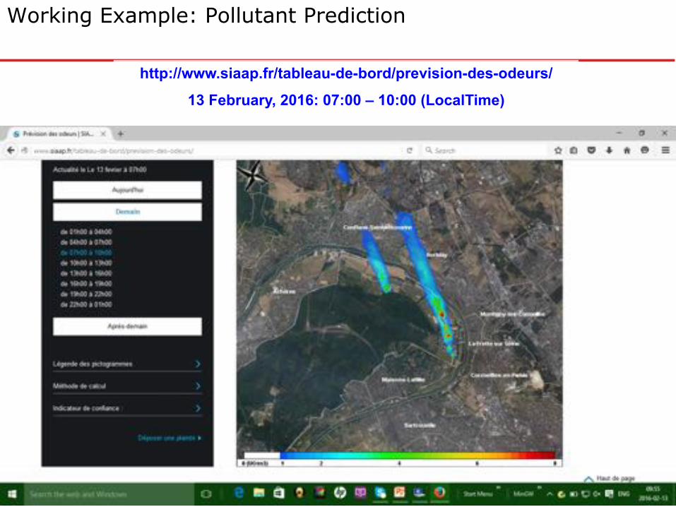
13 February, 2016: 07:00 – 10:00 (LocalTime)
Working Example: Pollutant Prediction
http://www.siaap.fr/tableau-de-bord/prevision-des-odeurs/
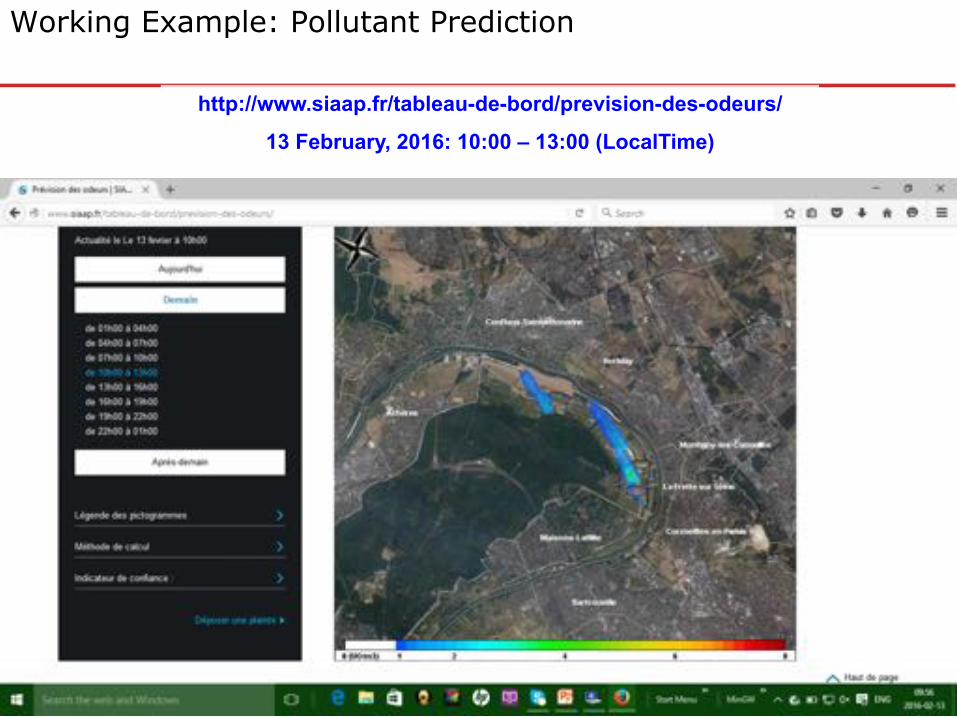
13 February, 2016: 10:00 – 13:00 (LocalTime)
Working Example: Pollutant Prediction

http://www.siaap.fr/tableau-de-bord/prevision-des-odeurs/
13 February, 2016: 13:00 – 16:00 (LocalTime)
Working Example: Pollutant Prediction
http://www.siaap.fr/tableau-de-bord/prevision-des-odeurs/
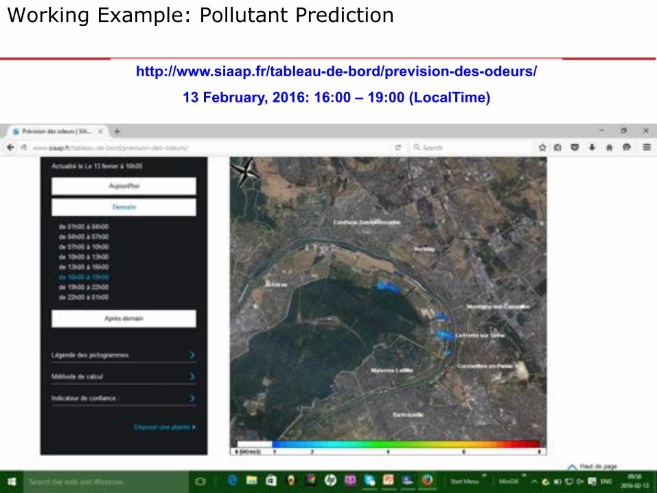
13 February, 2016: 16:00 – 19:00 (LocalTime)
Working Example: Pollutant Prediction

http://www.siaap.fr/tableau-de-bord/prevision-des-odeurs/
13 February, 2016: 19:00 – 22:00 (LocalTime)
Working Example: Pollutant Prediction

http://www.siaap.fr/tableau-de-bord/prevision-des-odeurs/
13 February, 2016: 22:00 – 01:00 (LocalTime)
Working Example: Pollutant Prediction
Guidelines
Increasing use of 3D CFD modelling for air quality assessment necessitates guidelines. For example, certain requirements stipulated by French Ministry of Environment are: • Validation of the numerical tool • Atmospheric stability class conservation over a 2-km domain • Grid independency (Variation of results <10% with grid factors of 0.8 and 1.2) • Proper meshing of obstacles (10 cells) • Cell aspect ratio less than 10 • Mesh orientation aligned with the wind • Numerical scheme of at least 2nd order of precision • Growth factor less than 1.2 between two cells • Wind profiles as defined by the WG • Boundary conditions far from zone of interest • Proper integration of the source term (geometry, temperature) • Modification of the wind field by the source, if applicable • Prandtl and Schmidt numbers equal to 0.7 • Proper turbulence model