CDS 101/110: Lecture 9-1 Frequency Domain...

CDS 101/110: Lecture 9-1 Frequency Domain Design

Richard M. Murray 26 November 2015

Goals: • Review canonical control design problem / std performance measures • Show how to use “loop shaping” to achieve a performance specification • Work through a simple example of a control design problem

Reading: • Åström and Murray, Feedback Systems, Ch 12

Richard M. Murray, Caltech CDSCDS 101/110, 23 Nov 2015

Design Patterns for Control Systems“Classical” control (1950s...)

• Goal: output y(t) should track reference trajectory r(t) • Design typically done in “frequency domain” (second half of CDS 101/110)

“Modern” (state space) control (1970s...)

• Goal unchanged: output y(t) should track reference trajectory r(t) [often constant]

2

• Reference input shaping • Feedback on output error • Compensator dynamics

shape closed loop response • Uncertainty in process

dynamics P(s) + external disturbances (d) & noise (n)

• Assume dynamics are given by linear system, with known A, B, C, D matrices • Measure the state of the

system and use this to modify the input • u = -K x + kr r

Richard M. Murray, Caltech CDSCDS 101/110, 23 Nov 2015 3

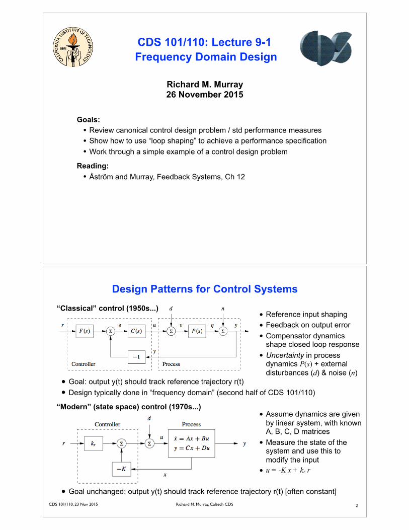
Input/Output Control Design Specifications

F(s) = 1: Four unique transfer functions define performance (“Gang of Four”) • Stability is always determined by 1/(1+PC) assuming stable process & controller

• Numerator determined by forward path between input and output

More generally: 6 primary transfer functions; simultaneous design of each • Controller C(s) enters in multiple places ⇒ hard to understand tradeoffs

Keep track all input/output transfer functions • Keep error small for all

reference signals r • Attenuate effect of sensor

noise n and disturbances d

• Avoid large input cmds u

Design represents a tradeoff between the quantities • Keep L=PC large for good

performance (Her << 1)

• Keep L=PC small for good noise rejection (Hηn < 1)

�

⇤�yu

⇥

⌅ =

�

⇧⇤

P1+PC � PC

1+PCPCF1+PC

P1+PC

11+PC

PCF1+PC

� PC1+PC � C

1+PCCF

1+PC

⇥

⌃⌅

�

⇤dnr

⇥

⌅


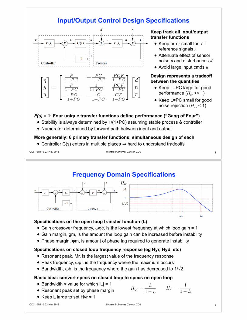
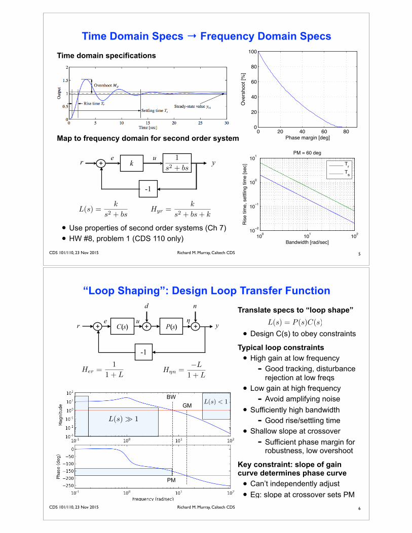
Frequency Domain Specifications

Specifications on the open loop transfer function (L) • Gain crossover frequency, ωgc, is the lowest frequency at which loop gain = 1 • Gain margin, gm, is the amount the loop gain can be increased before instability

• Phase margin, φm, is amount of phase lag required to generate instability

Specifications on closed loop frequency response (eg Hyr, Hyd, etc) • Resonant peak, Mr, is the largest value of the frequency response • Peak frequency, ωp , is the frequency where the maximum occurs • Bandwidth, ωb, is the frequency where the gain has decreased to 1/√2

Basic idea: convert specs on closed loop to specs on open loop • Bandwidth ≈ value for which |L| = 1 • Resonant peak set by phase margin

• Keep L large to set Hyr ≈ 1

4

|Hyr|

Her =1

1 + LHyr =

L

1 + L


Time domain specifications

Map to frequency domain for second order system

• Use properties of second order systems (Ch 7) • HW #8, problem 1 (CDS 110 only)

Time Domain Specs → Frequency Domain Specs

5

0 20 40 60 800

20

40

60

80

100

Phase margin [deg]

Ove

rsho

ot [%

]100 101 102

10−2

10−1

100

101

Bandwidth [rad/sec]R

ise

time,

set

tling

tim

e [s

ec]

PM = 60 deg

TrTs

k+ ye u

-1

r 1

s2 + bs

L(s) =k

s2 + bsHyr =

k

s2 + bs+ k


“Loop Shaping”: Design Loop Transfer Function

BW

L(s)� 1

L(s) < 1GM

PM

C(s) P(s)++

d

ηe u

-1

r +

n

y

Her =1

1 + L

L(s) = P (s)C(s)

H⌘n =�L

1 + L

Translate specs to “loop shape”

• Design C(s) to obey constraints

Typical loop constraints • High gain at low frequency

- Good tracking, disturbance rejection at low freqs

• Low gain at high frequency - Avoid amplifying noise

• Sufficiently high bandwidth - Good rise/settling time

• Shallow slope at crossover - Sufficient phase margin for

robustness, low overshoot

Key constraint: slope of gain curve determines phase curve • Can’t independently adjust

• Eg: slope at crossover sets PM


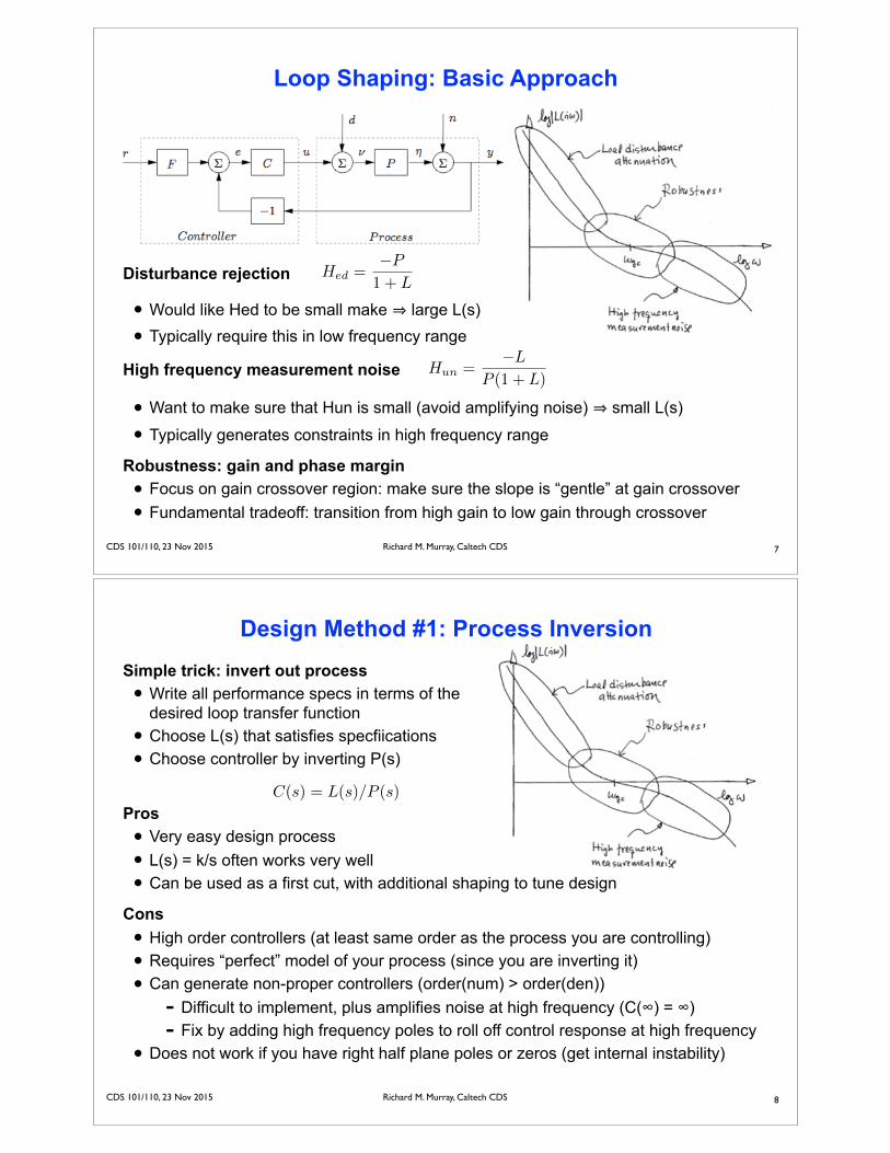
Loop Shaping: Basic Approach

Disturbance rejection

• Would like Hed to be small make ⇒ large L(s)

• Typically require this in low frequency range

High frequency measurement noise

• Want to make sure that Hun is small (avoid amplifying noise) ⇒ small L(s)

• Typically generates constraints in high frequency range

Robustness: gain and phase margin • Focus on gain crossover region: make sure the slope is “gentle” at gain crossover

• Fundamental tradeoff: transition from high gain to low gain through crossover

7

Hed =�P

1 + L

Hun =�L

P (1 + L)


Design Method #1: Process InversionSimple trick: invert out process • Write all performance specs in terms of the

desired loop transfer function • Choose L(s) that satisfies specfiications • Choose controller by inverting P(s)

Pros • Very easy design process • L(s) = k/s often works very well • Can be used as a first cut, with additional shaping to tune design

Cons • High order controllers (at least same order as the process you are controlling) • Requires “perfect” model of your process (since you are inverting it) • Can generate non-proper controllers (order(num) > order(den))

- Difficult to implement, plus amplifies noise at high frequency (C(∞) = ∞) - Fix by adding high frequency poles to roll off control response at high frequency

• Does not work if you have right half plane poles or zeros (get internal instability)

8

C(s) = L(s)/P (s)


-200

-100

0

100

10-1

100

101

102

103

-300

-200

-100

0

100

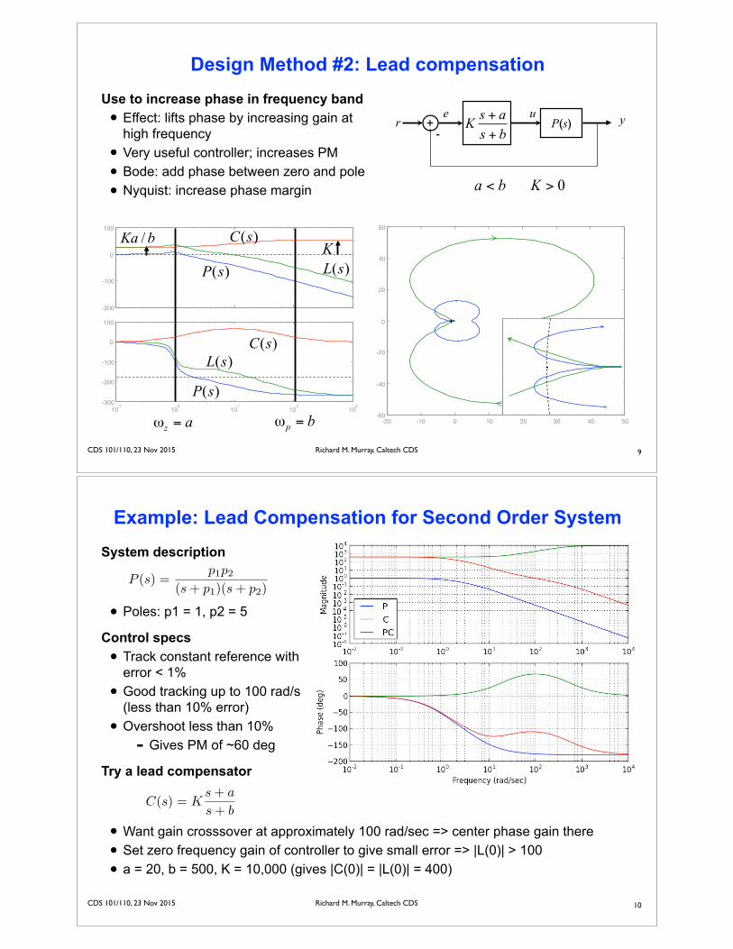
Design Method #2: Lead compensation

-20 -10 0 10 20 30 40 50-60

-40

-20

0

20

40

60

Use to increase phase in frequency band • Effect: lifts phase by increasing gain at

high frequency • Very useful controller; increases PM • Bode: add phase between zero and pole • Nyquist: increase phase margin

+-

r ye uP(s)


System description

• Poles: p1 = 1, p2 = 5

Control specs • Track constant reference with

error < 1% • Good tracking up to 100 rad/s

(less than 10% error) • Overshoot less than 10%

- Gives PM of ~60 deg

Try a lead compensator

• Want gain crosssover at approximately 100 rad/sec => center phase gain there • Set zero frequency gain of controller to give small error => |L(0)| > 100 • a = 20, b = 500, K = 10,000 (gives |C(0)| = |L(0)| = 400)

Example: Lead Compensation for Second Order System

10

P (s) =p1p2

(s+ p1)(s+ p2)

C(s) = Ks+ a

s+ b


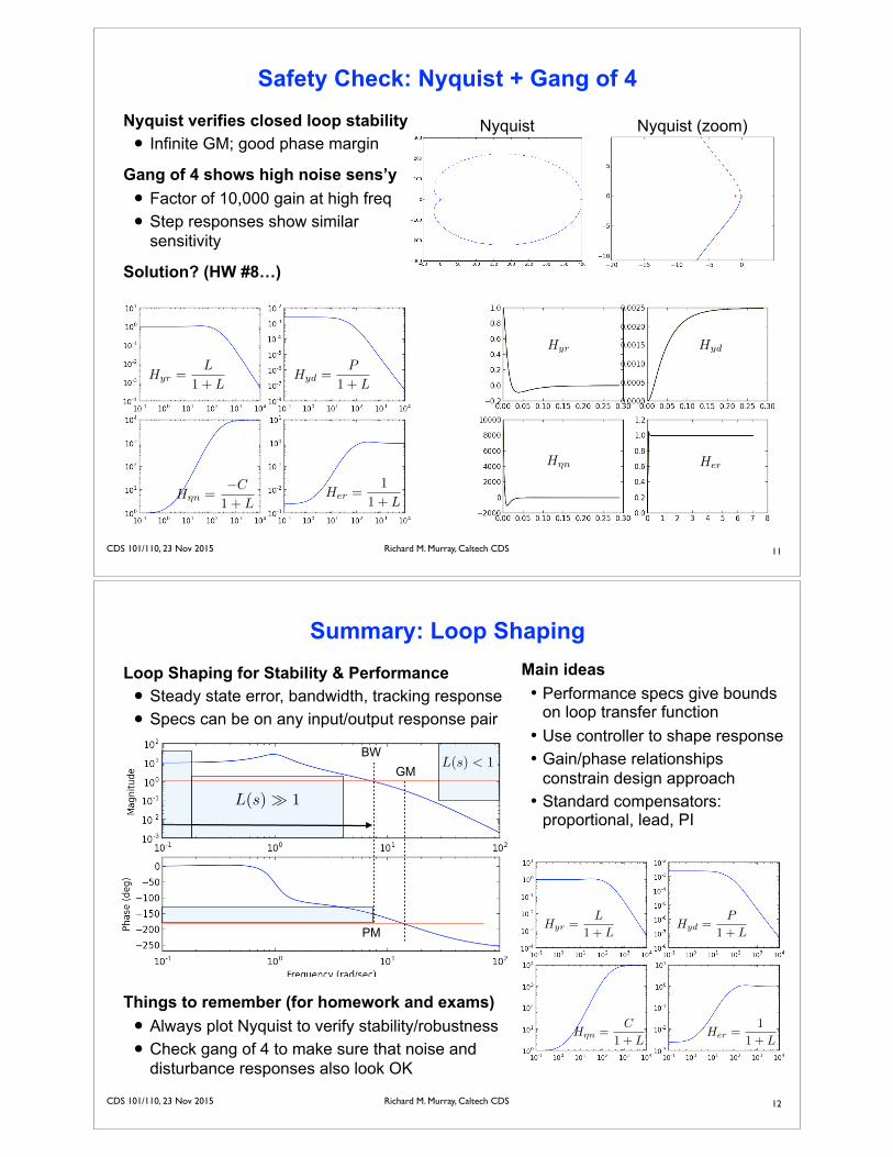
Nyquist Nyquist (zoom)Nyquist verifies closed loop stability • Infinite GM; good phase margin

Gang of 4 shows high noise sens’y • Factor of 10,000 gain at high freq • Step responses show similar

sensitivity

Solution? (HW #8…)

Safety Check: Nyquist + Gang of 4

11

H⌘n

Hyr Hyd

Her

Hyr =L

1 + L

Her =1

1 + L

Hyd =P

1 + L

H⌘n =�C

1 + L


BW

L(s)� 1

L(s) < 1GM

PM

12

Summary: Loop ShapingMain ideas � Performance specs give bounds

on loop transfer function � Use controller to shape response � Gain/phase relationships

constrain design approach � Standard compensators:

proportional, lead, PI

Hyr =L

1 + L

Her =1

1 + L

Hyd =P

1 + L

H⌘n =C

1 + L

Loop Shaping for Stability & Performance • Steady state error, bandwidth, tracking response • Specs can be on any input/output response pair

Things to remember (for homework and exams) • Always plot Nyquist to verify stability/robustness • Check gang of 4 to make sure that noise and

disturbance responses also look OK

CDS 101/110: Lecture 9-1 Frequency Domain...

Documents

Transcript of CDS 101/110: Lecture 9-1 Frequency Domain...