Cash-In-Advance

Randall Wright

1 Basic Assumptions

We begin with a very simple model: an endowment economy with homoge-

neous agents. The representative agent chooses a sequence for consumption

ct to solve

max∞Xt=0

βtu(ct),

subject to recursive budget and CIA constraints

ptct = ptet +mt + Tt −mt+1

ptct ≤ mt + Tt,

where pt is the nominal price level, et is the endowment,mt is money hodlings

at the begining of period t, and Tt is a transfer of money from the government,

that could be negative and that the agent regards as lump sum. The CIA

constraint requires that consumption be financed out of cash on hand at the

start of the period, including the transfer.1 In particular, one cannot use the

ptet dollars one receives from the sale of one’s endowment at t to finance ct;

it must be carried forward and used for ct+1.

There are different interpretations of this assumption. One that is similar

to a story Lucas proposed is as follows. First, each household consists of a

pair, say a “worker” and a “shopper.” Second, there are several types of

1Alternatively, one can assume Tt is not available that period, so that the CIA con-straint would be ptct ≤ mt; see below.

1

households, and each type lives in a distinct physical location, say an island.

To motivate gains from trade, assume that the consumption good comes in

K varieties, say different colors, and that each type produces good k but

wants to consume good k + 1 (modK). So each period “shoppers” of each

type k simultaneously take cash to the next island in order to purchase color

k + 1 consumption goods, while their “worker” partners — perhaps better

called “vendors,” really — stay home waiting to sell their endowment of color

k goods for money. Goods cannot be bartered directly if K > 2.2 Clearly,

cash aquired from today’s sales cannot be used until next period, since the

shopper leaves before the money rolls in. This motivates the CIA constraint.

What is relevant is the timing, not that households come in pairs; e.g., the

“vendor” agent can be replaced by “vending machine” that collects cash

while an individual is out shopping.

We can rewrite the CIA contraint using the budget constraint as mt+1 ≥ptet. Hence, the assumption can be reinterpretted as saying that agents are

forced to hold at least the nominal value of their endowment as money from

each period t into t+ 1. Although not usually stated this way, this makes it

pretty obvious what the CIA constraint is doing — simply imposing a demand

for money. The supply of money at t is denoted Mt, where the initial stock

M0 > 0 is given exogenously. The government budget constraint here is

T =M 0 −M . Formulating the problem in dynamic programing terms, after

eliminating ct, Bellman’s equation can be written

V (m) = maxm0

s.t. m0≥pe

½u

µe+

m+ T −m0

p

¶+ βV (m0)

¾,

where we surpress the time subscript and use a “prime” to indicate next

period (e.g., mt = m and mt+1 = m0). We ignore nonnegativity constraints

for now, but they will not bind in equilibrium here anyway. Also, we express

2In principle, goods could be traded indirectly, with perhaps some colors emerging ascommodity money; this can be ruled out simply by assuming that they cannot be stored(say, for more than one period).

2

the CIA constraint in real terms as m0/p ≥ e and let λ denote the Lagrange

multiplier, so that we can rewrite the problem as

V (m) = maxm0

½u

µe+

m+ T −m0

p

¶+ λ

µm0

p− e

¶+ βV (m0)

¾.

The usual dynamic programming arguments can be used to show that V

is differentiable and strictly concave; hence the solution to the maximization

problem is characterized by the first order condition

−u1(c)p

+λ

p+ βV 0(m0) = 0.

The envelope condition is V 0(m) = u1(c)/p. Updating this one period and

inserting into the previous equation, we have the Euler equation

u1(c)− λ =β

πu1(c

0),

where π = p0/p, so that π − 1 is the rate of inflation and 1/π the gross rateof return on money. An equilibrium here can be defined as a sequence for

(c,m, λ, p) satisfying the Euler equation, the CIA constraint, the government

budget constraint, and the market clearing conditions, c = e and m = M ,

at every date. Note that the government and individual budget constraints

together imply that as long as one of the two market clearing conditions

holds, the other holds automatically (Walras Law).

Using the fact that c = e at every date, in equilibrium, we write the Euler

equation as

λ = u1(e)−β

πu1(e

0).

Since the multipler λ must be nonnegative, we see that π ≥ βu0(e0)/u0(e) in

any equilibrium; as a special case, if e is constant then we must have π ≥ β in

any equilibrium. The CIA constraint is binding whenever π > βu0(e0)/u0(e),

in which case m0/p = c = e in equilibrium. Equating m0 = M 0, we see

that p = M 0/e at every date; i.e., the nominal price level is proportional

3

to next period’s money stock.3 Suppose e is constant, and consider the

money supply rule M 0 = µM , so that µ− 1 is the growth rate of M . Thenπ = p0/p = M 0/M = µ. More generally, if e is not constant, then inflation

is equal to the rate of monetary expansion minus the growth rate in e. In

any event, given any path for the money supply, this economy has a unique

monetary equilibrium, where c = e and p =M 0/e.4

In the above formulation there was no asset market, which is not restric-

tive because there can be no asset trading in equilibrium given a represen-

tative agent. However, as always, we could open up a bond market simply

to see what the bond prices or interest rates would have to be so that the

market cleared with no trades. Rewrite the budget equation as

pc = pe+m+ T −m0 + pbR− pb0,

where b is the number of bonds held at the start of the period, measured

in units of the consumption good, and R is the gross real rate of interest.

Agents start with b0 = 0. As is standard, the credit market clears (i.e., no

ones buys or sells bonds) as long as

R0 =u1(e)

βu1(e0).

Recall that λ ≥ 0 is equivalent to u1(e) ≥ βπu1(e

0), which we can now write

R0π ≥ 1. This is sometimes expressed as saying the nominal interest ratemust be positive, which follows as long as one defines the nominal rate i to

be R0π − 1.3If we alternatively assume that the transfer T is not available to satisfy the CIA

constraint that period, the same methods lead to p =M/e — i.e. the price level is propor-tional to the current money supply. Of course, this has no real implications in this simpleeconomy, since c = e at every date in either case.

4It is not so clear how to define a nonmonetary equilibrium here. Normally, one wouldsay that such an equilibrium is one where the value of money is 0 — i.e., p = ∞ — but inthis model, if p = ∞ the CIA constraint implies c = 0, and so markets do not clear. Itseems reasonable to say that p = ∞ constitutes a nonmonetary equilibrium despite thefact that c < e.

4

Of course, if e is constant then R0 = 1/β, and π/β ≥ 1 is a necessarycondition for equilibrium to exist, which puts constraints on feasible mon-

etary policies since π = µ. Hence, we can contract the money supply but

not faster than the rate implied by µ ≥ β. The intuitive reason is that if

we tried to set µ < β then agents would have incentive to set c < e and

store the difference in cash, since cash is appreciating faster than the rate of

time preference. Indeed, if we allow them to issue bonds (i.e., borrow), given

R = 1/β there would be arbitrage profits available. This is not crucial to

the result however: as we saw above, equilibrium requires u1(e) ≥ βπu1(e

0),

which can always be expressed as πR0 ≥ 1 by defining R0 = u1(e)/βu1(e0),

even if we do not allow bond trading. Notice that while this rules out π < β,

nothing rules out π > β; although π > β gives agents an incentive to set

c > e, the CIA constraint prevents them from doing so, and markets clear at

c = e.

2 Cash Goods and Credit Goods

Other than recognizing that there is a lower bound to the rate of monetary

contraction in equilibrium, there are of course no welfare implications to

monetary policy in the above example, because we always have c = e; there

is no margin that can be distorted to affect the real allocation, even though

prices do depend on the money supply. To make the analysis interesting

along this dimension, we need to give agents the opportunity to take some

more interesting decisions. A simple way to do this is to assume that there

are two goods, so that u(c) = u(c1, c2), but only c1 is subject to a CIA

constraint; sometimes c1 is called a cash good while c2 is called a credit good.

Moreover, for now assume that there is a linear technology for converting the

endowment good into either of the consumption goods, say e = c1 + c2; this

implies that in equilibrium the two consumption goods must have the same

price.

5

The constraints are

pc1 = pe− pc2 +m+ T −m0

pc1 ≤ m+ T,

since only c1 is subject to CIA. Eliminating c1 using the budget condition, the

CIA constraint becomes m0 ≥ pe− pc2; this says that any money generated

from the sale of e, if it is not spent on c2 must be held into the next period.

Again writing the constraing in real terms as m0/p ≥ e− c2 and letting λ be

the multipler, Bellman’s equation is

V (m) = maxm0,c2

½u

µe− c2 +

m+ T −m0

p, c2

¶+ λ

µm0

p− e+ c2

¶+ βV (m0)

¾.

As above, one can show that V is differentiable and strictly concave; hence, an

interior solution (we will consider corner solutions below) to the maximization

problem is characterized by the first order conditions

−u1(c)p

+λ

p+ βV 0(m0) = 0

−u1(c) + u2(c) + λ = 0.

The envelope condition is V 0(m) = u1(c)/p, which implies the Euler equation

u1(c)− λ =β

πu1(c

0).

While we discuss dynamic equilibria later, let us begin with the case where

the endowment e and the rate of monetary expansion µ are constant, and

look for steady state equilibria in which comsumption c and real balances

z = m/p are constant (so that prices evolve at the same rate as M). In

steady state, the Euler equation implies

λ = u1(c)

µ1− β

π

¶,

6

so that again we must have π ≥ β. Combining this with the other first order

condition, we have

E(c2) = u2(e− c2, c2)−β

πu1(e− c2, c2) = 0,

after inserting e− c2 = c1. A solution to this equation is an interior steady

state equilibrium as long as it satisfies the nonnegativity conditions strictly,

c2 ∈ (0, e).We could also have a corner solution in equilibrium. If u2(e, 0) ≤ β

πu1(e, 0)

then we have an equilibrium where only cash goods are consumed; in this

case things operate just like the previous model, with no credit goods. Alter-

natively, if u2(0, e) ≥ βπu1(0, e) then we have an equilibrium where no cash

goods are consumed and money is simply not valued. If these two inequal-

ities do not hold — which would be the case, e.g., as long as we impose the

standard curvature conditions u1(0, c2) = u2(c1, 0) = ∞ — then there exists

an interior monetary steady state, that is, a solution c2 ∈ (0, e) to E(c2) = 0.Differentiation implies E0 = β

πu11 − (1 + β

π)u12 + u22; this cannot be signed

for arbitrary values of π, but at π = β we know E0 < 0 for any concave u.

Hence, we can guarantee a unique equilibriuim for low inflation rates, but

not in general.

Summarizing, we have shown the following. First, there exists a monetary

steady state as long as u2(0, e) <βπu1(0, e), since it is only when u2(0, e) ≥

βπu1(0, e) that we have a corner solution where no cash goods are consumed.

A monetary steady state could be interior, or it could have only cash goods

consumed, which occurs when u2(e, 0) ≤ βπu1(e, 0). Thus, with low inflation

it is possible to have only cash goods consumed, with high inflation it is

possible to have only credit goods, and with intermediate inflation we have

both. Of course, curvature conditions like u2(e, 0) = u1(0, e) imply that both

goods are consumed for any π ≥ β. The monetary steady state is unique

if π is close to β, but we cannot guarantee this for a general π. We could

guarantee a unique steady state for any π if we assume u12 ≥ 0 (including

7

the case where u is separable), since then clearly E0 < 0. Actually, all we

really need is the weaker assumption that the marginal rate of substitution

along the line c1 = e− c2 is decreasing in c2:

∂

∂c2

u2(e− c2, c2)

u1(e− c2, c2)= u2u11 − (u1 + u2)u12 + u1u22 < 0. (1)

Since u2 =βπu1 in equilibrium, (1) says E0 < 0. Moreover, one can show that

(1) necessarily holds if both goods are normal, since c1 normal if and only if

u1u22 − u2u12 < 0 and c2 normal if and only if u2u11 − u1u12 < 0.5

Consider welfare. It should be obvious that efficiency requires u2 = u1

(solve the planner’s problemwithout the CIA constraint). Hence, the optimal

monetary policy requires π = β at every date, which means µ = β. This

policy a simple version of what is referred to as the Friedman rule, something

that will be encountered frequently in what follows. One way to interpret

such a policy is to say that it “undoes” the CIA constraint. It does so by

making agents “happy” to hold cash from one period to the next by effectively

giving money a rate of return equal to the rate of time preference. In principle

one could to do this by paying interest on currency, although presumably it

is administratively easier to contract the money supply, at least given that

we have recourse to nondistorting taxes (see below). Alternatively, if bonds

satisfied the CIA constraint, which is another way of saying that money pays

interest, one can support the efficient outcome by endowing the economy

with a fixed stock of bonds.6

5Consider maximizing u(c1, c2) subject to c1 + Pc2 = e. The first order condition is−Pu1 + u2 = 0, and the second order conditon always holds since Q = P 2u11 − 2Pu12 +u22 < 0. We have

∂c1∂e

= −Q−1µu2u1

u12 − u22

¶and

∂c2∂e

= −Q−1µu12 −

u2u1

u11

¶.

Since Q < 0, normal goods means u22 − u2u1u12 < 0 and u2

u1u11 − u12 < 0.

6Although we will not do do so explicitly here, one can introduce bonds (that do notsatisfy the CIA constraint) into the model with both cash and credit goods exactly as inthe model with only cash goods. As in that model, R0 = u2(c)/βu2(c

0) means that bonds

8

The situation is depicted in Figure 1 in terms of the trade off between c2at one date and c1 at the next date, since this is the interesting margin: an

agent who reduces consumption of the credit good today can keep the money

for one period when he can then consume more cash goods. An equilibrium

satisfies the marginal condition u2/βu1 = p/p0 = 1/π, as well as feasibility,

c2 = e − c1. Differentiation implies ∂c2/∂π is proportional to −E0, where

E(c2) was derived above. Again, E0 is ambiguous in general, but definitely

negative at π = β. Thus, near the optimal policy more inflation necessarily

increases the consumption of credit goods and reduces the consumption of

cash goods. One way to see it is to note that the function E shifts up with

an increase in π. If E0 < 0, which must be the case when π = β, there is a

unique equilibrium and ∂c2/∂π > 0. If there are multiple solutions to E = 0,

then of course E0 and therefore ∂c2/∂π alternates in sign across solutions.

Since E increases with π, the equilibria with π = β yields the lowest value

of c2 across any equilibria.7

Now consider dynamic equilibria. In general, a dynamic equilibrium sat-

isfies

u2(c1, c2) =β

πu1(c

01, c

02).

Suppose that π > β, so that the CIA constraint binds, at every date. Then

c1 = M 0/p = µM/p = µz, where z denotes real balances, and by feasibility

do not trade, which is necessary for equilibrium, and so in steady state we have R = 1/β.Given R0 = u2(c)/βu2(c

0), we can state the policy results as follows: µR0 ≥ 1 is necessaryfor equilibrium to exist, and the (efficient) policy is µR0 = 1.

7These effects can be illustrated using Figure 1. First, starting at the optimum, ifπ increases we need to find a point where an indifference curve is flatter on the linec2 = e − c1, which means moving southeast; hence, ∂c2/∂π > 0 at π = β. However,starting at an arbitrary equilibrium, the indifference can in principle become flatter as wemove in either direction along this line. Another way to say it is that starting with anarbitrary policy, ∂c2/∂π has a negative substitution effect and an ambiguous wealth effect,but at the optimal policy the wealth effect vanishes because ∂V/∂π = 0. The fact that c2is lowest at the optium π = β can also be seen by the fact that any intersection of the linec2 = e− c1 with an indifference curve that is flatter than this line must be to the right ofthe optimum. In particular, this implies is that in order for an increase in π to increasec1 and decrease c2, the increase in π must improve welfare.

9

Figure 1: Equilibrium with Cash and Credit Goods

c2 = e − µz. Moreover, π = p0/p = p0/M 0

p/µM= µz/z0. Hence, the previous

condition can be written

F (z, z0) = µzu2(µz, e− µz)− βz0u1(µz0, e− µz0) = 0.

This implicitly defines a difference equation z0 = f(z). An equilibrium is a

bounded solution to z0 = f(z) (it must be bounded for the usual reasons — if

not, and real balances become arbitrarily large, at some point the represen-

tative agent could get more utility from spending all of his money than he

could get in any equilibrium).

Notice that f(0) = 0, and that

dz0

dz= f 0(z) =

βu1 + βµz0(u11 − u12)

µu2 + µ2z(u21 − u22).

10

In particular, f 0(0) = βu1(0, e)/µu2(0, e), which means that f 0(0) < 1 if

and only if u2(0, e) <βµu1(0, e), which is the condition derived above that

guarantees there exists a monetary steady state. Figure 2 shows the situation

in the case where there exists a (unique) monetary steady state, z∗, which

means f 0(0) < 1, which means that f(z) cuts the 45o line from below at z∗.

This means that the monetary equilibrium is unstable, and the nonmonetary

equilibrium is stable. Hence, there always exist dynamic equilibria where we

start at some z0 ∈ (0, z∗) and z → 0. Indeed, if f 0(z) > 0, as shown, then for

any z0 ∈ (0, z∗) we have z → 0, and therefore there is an equilibrium where

real balances converge monotonically to 0 over time. we do not generate an

equilibrium if we start at z0 > z∗ in this case (where f 0 > 0), since then z

becomes unbounded.

We need to check one detail concerning the dynamic paths for z described

above — and that is we need to verify that the CIA constraint binds at all

points along the path, as we have assumed in the argument. Note that CIA

binds if and only if λ > 0, where

λ = u1(µz, e− µz)− u2(µz, e− µz)

at each point in time, from the first order conditions. Since this expression is

unambiguously decreasing in z, if λ > 0 at some z then λ > 0 for all z < z.

At the steady state z∗, we have u2 =βµu1, and so as we established earlier

λ > 0 in steady state as long as µ > β. Hence, when z < z∗ along the entire

path, as when f 0 > 0 and z0 ∈ (0, z0), we know that λ > 0 along the entire

path.

If f 0 > 0 does not hold, even more interesting outcomes are possible. For

example, if f 0(z∗) < 0 then z oscillates around z∗, and if f−1 has a slope

less than −1 at z∗ then z0 = f(z) will display limit cycles around z∗, by

the standard arguments (see, e.g., Azariadis). This is displayed in Figure 3;

clearly, if f−1 has slope less than −1 at z∗ then f and f−1 must intersect

not only at z∗, but also at (zL, zH), say; hence, zL = f(zH) and zH = f(zL).

11

Figure 2: Dynamic Equilibria with f 0 > 0

Of course, given that z is not monotone decreasing, the above argument to

establish that λ > 0 along the entire path does not work. However, since

µ > β implies λ > 0 at steady state z∗, continuity implies that λ > 0 for all

z < z for some z > z∗. Hence, we can construct equilibria where z cycles

and the CIA constraint is binding at every date at least as long as the cycle

is not too big.

Consider the following example:

u(c) =(b+ c1)

1−α

1− α+ c2,

12

where α > 0. For this case, F (z, z0) = 0 can be solved explicity for

z = f−1(z0) =βz0

µ (b+ µz0)α,

and for the steady state

z∗ =

³βµ

´1/α− b

µ.

Moreover, λ = u1−u2 = (b+ µz)−α−1 > 0 as long as z < z = (1−b)/µ > z∗

(assuming µ > β). For example, if µ = 3, β = 0.95, b = 0.47, and α = 5,

a two period cycle emerges around the steady state z∗ = 0.108, where z

fluctuates between approximately zL = 0.072 and zH = 0.151. Since z =

0.177, CIA binds at zL and zH . Indeed, in the figure, where we start at z0just below z and watch z converge to the cycle, CIA binds along the entire

path.8

3 Endogenous Labor

One intuitive breakdown of goods into cash and credit goods is to say that

consumption of one’s own leisure does not require cash, while consumption

of market goods does. Although such a model is basically a reinterpretation

of what we have already seen in the model with cash and credit goods, it

is worth considering since it is one popular specification in the literature.

Suppose u = u(c, 1− h), where c is consumption and subject to CIA, while

h is hours worked so that (by normalizing total time to 1) we can interpret

1− h as lesiure. Let the nominal wage be w; the real wage is of course w/p,

and will be determined below. The idea here will be that workers get paid

in nominal wages that cannot be spent in the current period, but everything

goes through exactly the same, if instead we say that they are paid in real

8The construction of the cycle used the fact that, in this example, the slope of f−1 atz∗is easily calculated to be

£1− α+ αb(µ/β)1/α

¤−1, which equals −1 at b = (β/µ)1/α(α−

2)/α. In the neigborhood of this value of b, a two period cycle emerges.

13

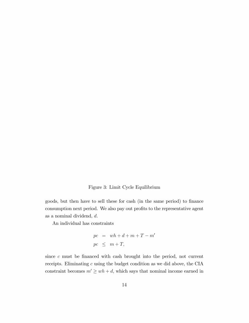
Figure 3: Limit Cycle Equilibrium

goods, but then have to sell these for cash (in the same period) to finance

consumption next period. We also pay out profits to the representative agent

as a nominal dividend, d.

An individual has constraints

pc = wh+ d+m+ T −m0

pc ≤ m+ T,

since c must be financed with cash brought into the period, not current

receipts. Eliminating c using the budget condition as we did above, the CIA

constraint becomes m0 ≥ wh+ d, which says that nominal income earned in

14

one period must be held as money into the next period. As above, we can

write the constraint in real terms as m0

p≥ w

ph + d

p, and Bellman’s equation

becomes

V (m) = maxm0,h

½u

µwh+ d+m+ T −m0

p, 1− h

¶+λ

µm0 − wh− d

p

¶+ βV (m0)

¾.

The first order conditions are

−u1(c, 1− h)

p+

λ

p+ βV 0(m0) = 0

w

pu1(c, 1− h)− u2(c, 1− h)− w

pλ = 0.

Using V 0(m) = u1(c, 1− h)/p, we can write the first of these as

u1(c, 1− h)− λ =β

πu1(c

0, 1− h0).

The obvious equilibrium conditions for competitive firms imply w = pf 0(h)

and d = pf(h)− wh, and then the budget equation implies c = f(h); hence

we can write the other first order condtion as

f 0(h) [u1(c, 1− h)− λ] = u2(c, 1− h),

where c = f(h). Combing these two equations, we have

u2(c, 1− h) =β

πu1(c

0, 1− h0)f 0(h). (2)

Things are very much analogous to the previous model, except that now the

relevant trade off can be said to be between leisure today and consumption

tomorrow, since working today yields money income that must be carried

over one period before it can be turned into consumption. In particular, in

a steady state we must have π ≥ β. Also, efficiency implies π = β.

15

One difference from the previous model is that the relative price of leisure,

the real wage, is endogenous here since w = pf 0(h), while the relative price

of credit goods in terms of cash was fixed at 1. Of course, one could augment

the previous model, say by assuming c1 = g(c2) instead of the extreme case

c1 = e−c2. In any case, having the price endogenous complicates things onlya little. For example, ∂h/∂π now takes the same sign as

βu1f00 + βf 02u11 − (β + π)f 0u12 + πu22,

where the first term accounts for the equilibrium change in wages while the

rest of the terms are analogous to the expression for ∂c2/∂π. Hence, at least

at the optimum π = β, we know that hours are decreasing in π. Moreover, h

is maximized at π = β (not only locally, but globally, by the same argument

that told us c2 is minimized globally at π = β).

One reason to interpret the credit good as leisure is that we can bring firms

into the picture in a more interesting way. In particular, suppose we change

the model by saying that consumers do not have a CIA constraint at all, but

firms do. Thus, consumers maximize subject only to the budget equation

pc = hw + d at every date. In particular, notice that since consumers are

not constrained to hold money, they never do, so m does not appear in their

problem.9 Hence, workers solve a sequence of static problems, the solution to

which is characterized by the first order condition wpu1(c, 1−h) = u2(c, 1−h)

at each date. Since c = f(h) in equilibrium, this condition can be solved for

h at each point in time. Of course, given an arbitrary interest rate consumers

might also like to save or borrow so as to smooth consumption over time, but

this will not be possible in equilibrium, because we have homogeneous agents.

As usual, interest rates will adjust so that u1(c, 1 − h) = βR0u1(c0, 1 − h0),

and no lending or borrowing takes place, which means that we can solve the

9Also, here we give all transfers of new money to firms, so T does not appear in theconsumer problem either. This is merely for notational convenience, however; it wouldbe equivalent to give these transfers to consumers, who would simply spend them in eachperiod.

16

consumer problem as described above.

The firm problem, however, now explicitly contains dynamic elements

due to their CIA constraint. As is standard, we assume that they maximize

the (real) present discounted value of their dividend stream,P

∆tdtpt, where

∆t = 1/(R1 · · ·Rt) is the relative price of a unit of consumption at t in terms

of date 0 goods, under the interpretation of Rt as the gross interest rate

on a one-period bond maturing at t. Firms are subject to two constraints.

First, d = pf(h)−wh+m+ T −m0, since dividends must come from either

profits or adjustments to their money inventories. Second, they face the CIA

constraint wh ≤ m + T , which says that they must pay nominal wages out

of cash on hand at the start of the period (and not out of cash receipts from

sales within the period). Writing the CIA constraint in real terms, Bellman’s

equation becomes

V (m) = maxm0,h

½pf(h)− wh+m+ T −m0

p+ λ

µm+ T − wh

p

¶+1

R0V (m0)

¾where the effective discount factor is ∆0/∆ = 1/R0.

The first order conditions imply

−1p+

V 0(m0)

R0= 0

f 0(h)− w

p− λ

w

p= 0.

As V 0(m) = (1 + λ)/p, the first equation can be written πR0 = 1+ λ0, which

again implies πR0 ≥ 1 as a necessary condition for equilibrium. The otherfirst order condition can now be rearranged as

f 0(h0) =w0

p0(1 + λ0) =

w0

p0πR0.

From the consumers problem, w0

p0 =u2(c0,1−h0)u1(c0,1−h0) and R0 = u1(c,1−h)

βu1(c0,1−h0) . Hence,

equilibrium satisfies

u2(c0, 1− h0) =

β

π

u1(c0, 1− h0)2

u1(c, 1− h)f 0(h0). (3)

17

Notice that this is different from the equilibrium condition when CIA is

imposed on consumers, given by (2).

The intuition is as follows. In the case of CIA on consumers the relevant

trade off for an individual is between leisure today and consumption tomor-

row, by analogy to the trade off between credit goods today and cash goods

tomorrow depicted in Figure 1. The MRS is u2(c,1−h)βu1(c0,1−h0) , while the MRT is

f 0(h)πsince by giving up a unit of leisure one acquires f 0(h) units of output

today that can be used to buy 1/π units of consumption tomorrow. Equating

MRS and MRT yields (2). With CIA on firms, however, the relevant trade

off is between consumption today and consumption tomorrow. The MRS isu1(c,1−h)

βu1(c0,1−h0) , while the MRT isu1(c0,1−h0)u2(c0,1−h0)

f 0(h0)π, since by giving up one unit of

consumption today through lower real dividends, a shareholder allows the

firm to hire u1(c0,1−h0)u2(c0,1−h0)

1πunits of labor next period, which then yields f 0(h0)

units of output. Equating MRS and MRT in this case yields (3). Despite all

this, it is quite interesting that the steady state implications are identical,

since in steady state (2) and (3) reduce to the same thing.

4 Investment and Growth

We want to consider economies with capital. A simple set up is provided

by the model with a linear technology, y = f(k) = Bk (we ignore labor for

the moment), which is interesting because it can generate long run growth.

Also, let A = B + 1− δ, where δ is the depreciation rate on capital, so that

feasibility can be written c = f(k)+(1−δ)k−k0 = Ak−k0. As a benchmark,let us review the case where there is no money. Then the equilibrium will be

efficient and solve the planner’s problem described by

V (k) = maxk0{u (Ak − k0) + βV (k0)} .

Assuming an iterior solution (we will check this below), the first order condi-

tion is u0(Ak−k0) = βV 0(k0), the envelope condition is βV 0(k) = Au0(Ak−k0),

18

and so the Euler equation is

u0(c) = βAu0(c0).

Since c = Ak − k0, this is a second order difference equation in k, which

has many solutions given the single initial condition k0. The unique optimal

path for k is the solution that also satisfies the usual transversality condition

(TVC), which here we write as limT→∞ βTu0(AkT − kT+1)kT+1 = 0.

We are interested in a balanced growth path — that is, a solution to the

above problem where k grows at a constant rate: k0 = γk, which implies

c0 = γc. It is well known that this does not obtain for arbitrary preferences,

and only in the case of constant relative risk aversion (CRRA), u(c) = c1−σ−11−σ .

Given this utility function, and given balanced growth, the Euler equation

becomes

c−σ = βA(γc)−σ,

which simplifies to γ = (βA)1/σ. Hence, the Euler equation is satisfied by

the balanced growth path k0 = γk with γ = (βA)1/σ. We have kt = γtk0

for all t, and the net growth rate is positive if γ > 1, which means βA > 1.

The TVC holds if βγ < 1, which means β1+σA > 1 (notice that this implies

c = Ak − k0 > 0 automatically). So, we simply assume that β < A−1/(1+σ),

so that TVC holds (as is nonnegativity), and then observe that there are still

two cases: β < A−1 implies γ < 1, so k → 0, and β > A−1 implies γ > 1, so

k grows without bound.10

Now consider the same economy with a CIA constraint on consumption,

but for now not investment. Using the fact that the equilibrium interest rate

(from the profit maximization condition) must be r = B, so that [r + (1 −δ)]k = Ak, the budget and cash constraints are

pc = pAk − pk0 +m+ T −m0

pc ≤ m+ T.

10Notice that in this model we converge to the balanced growth path immediately —that is, kt+1 = γkt from the very first period.

19

As usual, we combine these to write CIA asm0 ≥ p(Ak−k0). Hence, we have

V (k,m) = maxk0,m0

½u

µAk − k0 +

m+ T −m0

p

¶+ λ

µm0

p+ k0 −Ak

¶+ βV (k0,m0)

¾.

The first order conditions are u0(c) − λ = βV1(k0,m0) and u0(c) − λ =

pβV2(k0,m0), the envelope conditions are V1(k,m) = Au0(c)−Aλ and V2(k,m) =

u0(c)/p, and so the Euler equations are

u0(c)− λ = βA [u0(c0)− λ0]

u0(c)− λ =β

πu0(c0).

Togther these imply (πA − 1)u0(c0) = πAλ0, and so we see that πA ≥ 1 isnecessary for equilibrium. Recalling that A = r, this is the same as the

condition we saw in the other models, πr ≥ 1.Solving the second Euler equation for λ and inserting into the first yields

βπu0(c0) = βA β

π0u0(c00), or

u0(c0) = βAπ

π0u0(c00).

Hence, at least if π is constant, we have u0(c) = βAu0(c0) at every date,

which is identical to the equilibrium condition from the model with no CIA

constraint. That is, given CRRA utility, equilibrium in the model with CIA

is given by the same balanced growth path we had without CIA, with γ =

(βA)1/σ. Moreover, given M 0 = µM , the CIA condition at equality implies

c = µM/p = µz. So on the balance growth path z0 = γz, and therefore

π = µ/γ (the inflation rate is the rate of monetary expansion minus the

economic growth rate). This means that the condition πA ≥ 1 becomes

µ ≥ β1/σA(1−σ)/σ. This puts a bound on how fast we can contract the

money supply, but otherwise there are no implications for policy: as long as

µ satisfies this condition, the equilibrium in independent of µ and identical

to the model without CIA.

Stockman pointed out that the above very strong implication follows be-

cause we have CIA on consumption only (although he did so in a different

20

model, with a steady state rather than a balanced growth path, which we

analyze below). Consider imposing CIA on consumption and investment:

pc + p(k0 − k) ≤ m+ T . As usual, we use the budget equation to write the

CIA constraint as m0

p≥ Ak − k, which contrasts with the previous model

with CIA only on consumption, where m0

p≥ Ak − k0. We assume A > 1.11

The Bellman equation is

V (k,m) = maxk0,m0

½u

µAk − k0 +

m+ T −m0

p

¶+ λ

µm0

p+ k −Ak

¶+ βV (k0,m0)

¾.

The first order conditions are u0(c) = βV1(k0,m0) and u0(c)−λ = pβV2(k

0,m0),

the envelope conditions are V1(k,m) = Au0(c) − (A − 1)λ and V2(k,m) =

u0(c)/p, and so the Euler equations are

u0(c)− βλ0 = βA [u0(c0)− λ0]

u0(c)− λ =β

πu0(c0).

The second Euler equation is the same as in the model with CIA on c

only, but the first Euler equation is different. Eliminating λ now leads to

u0(c0) = βu0(c0) +β2(A− 1)

πu0(c00).

Assuming CRRA utility and balanced growth, this can be written

c−σ = β(γc)−σ +β2(A− 1)

π

¡γ2c¢−σ

,

which is a quadratic in γσ and has solution

γσ =β

2

h1 +

p1 + 4(A− 1)/π

i.

Hence, the growth rate is decreasing in π. As above, π = µ/γ, which in

principle we could insert into this equation to solve for γ as a function of µ;

11Recalling that A = B+1− δ, CIA implies here that (B− δ)k, and so the assumptionis B > δ.

21

alternatively, we could think of the policy as the direct choice of π, which

implies γ and then µ endogensouly. In any case, recalling that the equilibrium

without CIA is γσ = βA, the efficient policy can be seen to be πA = 1

or µ = β1/σA(1−σ)/σ. Moreover, CRRA implies λ = c−σ(1 − γ−σβ/π), or

π ≥ βγ−σ, which combines with the above solution for γ to yield πA ≥ 1 orµ ≥ β1/σA(1−σ)/σ in any equilibrium, analogous to what we found earlier.

The bottom line is when we impose CIA on consumption only then the

rate of monetary expansion µ is neutral, but when we impose CIA on con-

sumption plus investment µ affects the allocation. We leave is as an exrcise

to show that if we have CIA on investment only then the outcome is the same

as CIA on consumption plus investment (not too surprsingly, given that CIA

on consumption only did not matter). Intuitively, CIA on consumption only

cannot be avoided, since the only alternative to consumption is investment,

and investment merely creates future output that still cannot be consumed

without holding cash for one period. Hence, CIA on consumption does not

distort any decisions. By contrast, CIA on investment does distort decisions,

since one can aviod it by consuming more and saving less. As usual, in

this case the optimal policy is the Friedman rule, which is to deflate so that

πA = 1, which effectively undoes the CIA constraint.

Of course, if we impose CIA only on consumption, but assume credit

goods or leisure that are not subject to CIA as well as cash goods that

are, policy will matter in this model, just as it did in the models without

capital. For instance, suppose u = u(c, 1 − h) and y = A(h)k. Notice

that since this technology displays increasing returns, we do not assume

agents rent labor and capital in competitive factor markets here, because

profit maximization will not be well defined. Rather, we assume agents

operate their own individual technologies.12 Their resource constraint is c =

12To motivate this, consider a static (nonmonetary) economy. If competitive firmsmaximize profit A(h)k−wh− rk, the second order conditions fail. However, if individualsmaximize V = u[A(h)k − k0, 1 − h] + βv(k0), where here v is an (exogenous) increasingand concave function, the problem is well behaved. To see this, note that the first order

22

A(h)k−k0+(m+T−m0)/p, and for now we impose CIA only on consumption,

pc ≤ m+T , which becomes m0/p ≥ A(h)k−k0 using the resource constraint.Hence, we have

V (k,m) = maxk0,m0,h

½u

∙A(h)k − k0 +

m+ T −m0

p, 1− h

¸+λ

∙m0

p+ k0 −A(h)k

¸+ βV (k0,m0)

¾.

The usual methods yield a first order condition for h and two Euler equations

for k and m, which we write as

u1(c, 1− h)− λ = u2(c, 1− h)/kA0(h)

u1(c, 1− h)− λ = βA(h0) [u1(c0, 1− h0)− λ0]

u1(c, 1− h)− λ =β

πu1(c

0, 1− h0).

Proceeding as always, the two Euler equations imply λ0 = u1(c0, 1 −

h0)[ 1πA(h0) − 1], and so πA(h0) ≥ 1 in any equilibrium. By eliminating λ

the Euler equations also imply

u1(c0, 1− h0) = βA(h0)

π

π0u1(c

00, 1− h00),

which is of the same form as the equilibrium condition in the basic model

with CIA on c only; in particular, if π is constant we have u1(c, 1 − h) =

βA(h)u1(c0, 1−h0). Therefore, investment is efficient if and only if h is at its

efficient level, h∗. However, the above also imply

u2(c, 1− h) = kA0(h)β

πu1(c

0, 1− h0),

which generally distorts the labor decision here for exactly the same reason

it does in the model without capital — recall (2). We leave it as an exercise

conditions are V1 = −u1 + βv0 = 0 and V2 = u1kA0 − u2 = 0, and the second order

conditions are V11 = u11 + βv00 < 0, V22 = (kA0)2u11 − 2(kA0)u12 + u22 < 0, and (aftersimplification) V11V22 − V 2

12 = u11u22 − u212 + βv00V22 > 0.

23

to work out equilibrium for the case where preferences satisfiy the balanced

growth conditions for an economy with endogenous labor — that is, c0 = γc

and h constant — which means that either u = c1−σ

1−σ v(1− h), or u = log(c) +

v(1− h), for some well behaved function v — and to show that the Friedman

rule is once again efficient.

One can consider other combinations of the above models. For instance,

consider endogenous labor with CIA on investment only, m+Tp≥ k0− k. The

usual methods now lead to the equilibrium conditions

u1(c, 1− h) = u2(c, 1− h)/kA0(h)

u1(c, 1− h) + λ = β [A(h0)u1(c0, 1− h0) + λ0]

u1(c, 1− h) =β

πu1(c

0, 1− h0).

Or, consider cash and credit goods in the growth model. The equilibrium

conditions are now

u1(c1, c2)− λ = u2(c01, c

02)

u1(c1, c2)− λ = βA(h0) [u1(c01, c

02)− λ0]

u1(c1, c2)− λ =β

πu1(c

01, c

02).

We leave it as an exercise to find γ under the assumption that preferences

generate balanced growth, to explore the effect of an increase in π on γ

and h, and to show that the Friedman rule continues to be efficient in these

models.13

One could also work with a more standard production function, say y =

f(k, h), as much of the literature does. For example, suppose we impose

CIA on consumpton only, pc ≤ m + T . The budget constraint is pc =

wh + p(r + 1 − δ)k + d − pk0 +m + T −m0, where d represents (nominal)

13Note that the balanced growth conditions are different in these two cases: with endoge-nous labor, we want c0 = γc and h0 = h; with cash and credit goods, we would presumablywant c01 = γc1 and c02 = γc2.

24

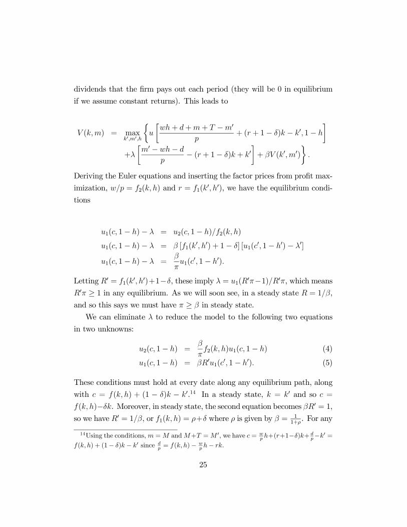
dividends that the firm pays out each period (they will be 0 in equilibrium

if we assume constant returns). This leads to

V (k,m) = maxk0,m0,h

½u

∙wh+ d+m+ T −m0

p+ (r + 1− δ)k − k0, 1− h

¸+λ

∙m0 − wh− d

p− (r + 1− δ)k + k0

¸+ βV (k0,m0)

¾.

Deriving the Euler equations and inserting the factor prices from profit max-

imization, w/p = f2(k, h) and r = f1(k0, h0), we have the equilibrium condi-

tions

u1(c, 1− h)− λ = u2(c, 1− h)/f2(k, h)

u1(c, 1− h)− λ = β [f1(k0, h0) + 1− δ] [u1(c

0, 1− h0)− λ0]

u1(c, 1− h)− λ =β

πu1(c

0, 1− h0).

Letting R0 = f1(k0, h0)+1−δ, these imply λ = u1(R

0π−1)/R0π, which meansR0π ≥ 1 in any equilibrium. As we will soon see, in a steady state R = 1/β,and so this says we must have π ≥ β in steady state.

We can eliminate λ to reduce the model to the following two equations

in two unknowns:

u2(c, 1− h) =β

πf2(k, h)u1(c, 1− h) (4)

u1(c, 1− h) = βR0u1(c0, 1− h0). (5)

These conditions must hold at every date along any equilibrium path, along

with c = f(k, h) + (1 − δ)k − k0.14 In a steady state, k = k0 and so c =

f(k, h)−δk. Moreover, in steady state, the second equation becomes βR0 = 1,so we have R0 = 1/β, or f1(k, h) = ρ+δ where ρ is given by β = 1

1+ρ. For any

14Using the conditions,m =M andM+T =M 0, we have c = wp h+(r+1−δ)k+

dp−k0 =

f(k, h) + (1− δ)k − k0 since dp = f(k, h)− w

p h− rk.

25

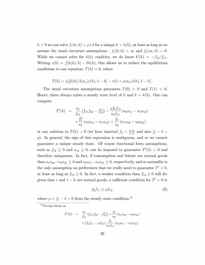
h > 0 we can solve f1(k, h) = ρ+δ for a unique k = k(h), at least as long as we

assume the usual curvature assumptions , f1(0, h) = ∞ and f1(∞, h) = 0.

While we cannot solve for k(h) explicity, we do know k0(h) = −f12/f11.Writing c(h) = f [k(h), h] − δk(h), this allows us to reduce the equilibrium

conditions to one equation, T (h) = 0, where

T (h) = f2[k(h), h]u1 [c(h), 1− h]− π(1 + ρ)u2 [c(h), 1− h] .

The usual curvature assumptions guarantee T (0) > 0 and T (1) < 0.

Hence, there always exists a steady state level of h and k = k(h). One can

compute

T 0(h) =u1f11

¡f11f22 − f212

¢− ρf2f12

u2f11(u2u11 − u1u12)

+f22u2(u2u11 − u1u12) +

f2u2(u1u22 − u2u21)

at any solution to T (h) = 0 (we have inserted f2 =πβu2u1and also f1 − δ =

ρ). In general, the sign of this expression is ambiguous, and so we cannot

guarantee a unique steady state. Of course functional form assumptions,

such as f12 ≥ 0 and u12 ≥ 0, can be imposed to guarantee T 0(h) < 0 and

therefore uniqueness. In fact, if consumption and leisure are normal goods

then u1u22−u2u21 ≤ 0 and u2u11−u1u12 ≤ 0, respectively, and so normality isthe only assumption on preferences that we really need to guarantee T 0 < 0,

at least as long as f12 ≥ 0. In fact, a weaker condition than f12 ≥ 0 will do:given that c and 1− h are normal goods, a sufficient condition for T 0 < 0 is

f2f11 ≤ ρf12, (6)

where ρ = f1 − δ > 0 from the steady state condition.15

15Group terms as

T 0(h) =u1f11

¡f11f22 − f212

¢+

f2u2(u1u22 − u2u21)

+ (f2f11 − ρf12)f2

u2f11(u2u11 − u1u12) .

26

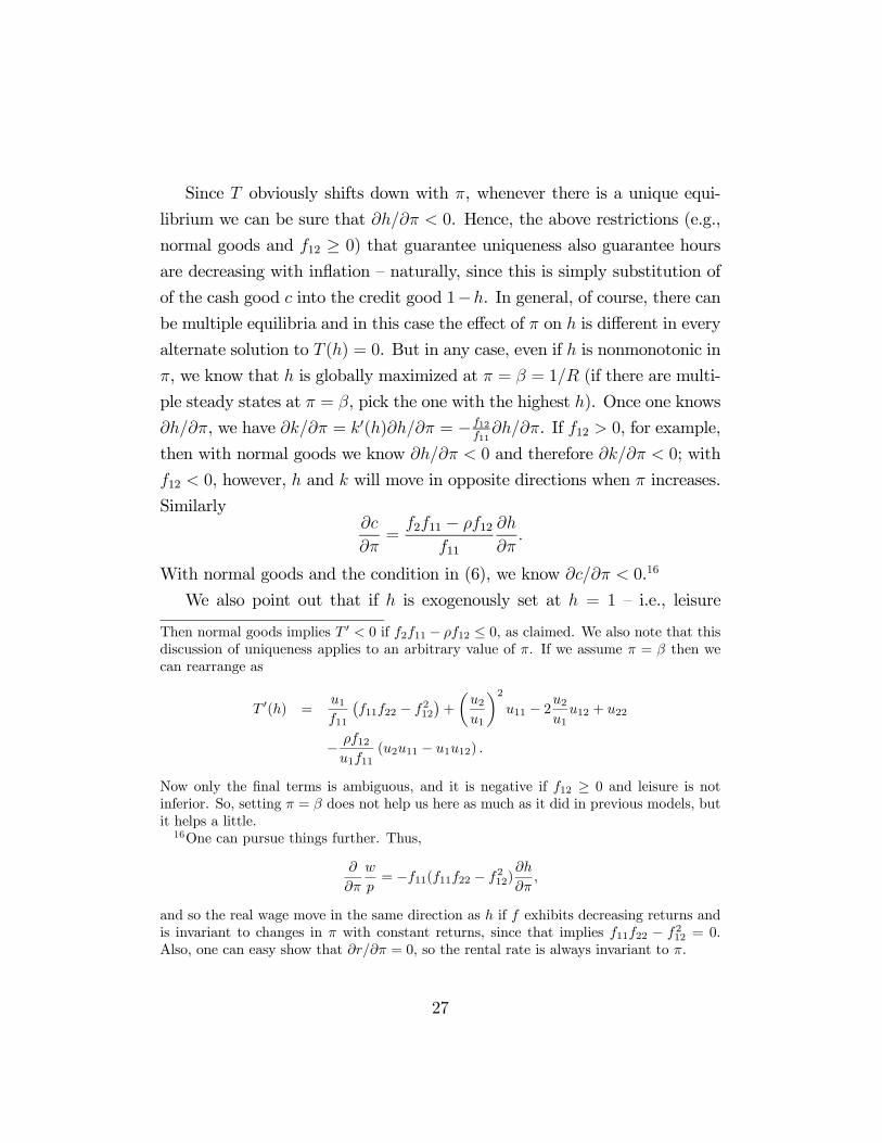
Since T obviously shifts down with π, whenever there is a unique equi-

librium we can be sure that ∂h/∂π < 0. Hence, the above restrictions (e.g.,

normal goods and f12 ≥ 0) that guarantee uniqueness also guarantee hoursare decreasing with inflation — naturally, since this is simply substitution of

of the cash good c into the credit good 1−h. In general, of course, there can

be multiple equilibria and in this case the effect of π on h is different in every

alternate solution to T (h) = 0. But in any case, even if h is nonmonotonic in

π, we know that h is globally maximized at π = β = 1/R (if there are multi-

ple steady states at π = β, pick the one with the highest h). Once one knows

∂h/∂π, we have ∂k/∂π = k0(h)∂h/∂π = −f12f11

∂h/∂π. If f12 > 0, for example,

then with normal goods we know ∂h/∂π < 0 and therefore ∂k/∂π < 0; with

f12 < 0, however, h and k will move in opposite directions when π increases.

Similarly∂c

∂π=

f2f11 − ρf12f11

∂h

∂π.

With normal goods and the condition in (6), we know ∂c/∂π < 0.16

We also point out that if h is exogenously set at h = 1 — i.e., leisure

Then normal goods implies T 0 < 0 if f2f11 − ρf12 ≤ 0, as claimed. We also note that thisdiscussion of uniqueness applies to an arbitrary value of π. If we assume π = β then wecan rearrange as

T 0(h) =u1f11

¡f11f22 − f212

¢+

µu2u1

¶2u11 − 2

u2u1

u12 + u22

− ρf12u1f11

(u2u11 − u1u12) .

Now only the final terms is ambiguous, and it is negative if f12 ≥ 0 and leisure is notinferior. So, setting π = β does not help us here as much as it did in previous models, butit helps a little.16One can pursue things further. Thus,

∂

∂π

w

p= −f11(f11f22 − f212)

∂h

∂π,

and so the real wage move in the same direction as h if f exhibits decreasing returns andis invariant to changes in π with constant returns, since that implies f11f22 − f212 = 0.Also, one can easy show that ∂r/∂π = 0, so the rental rate is always invariant to π.

27

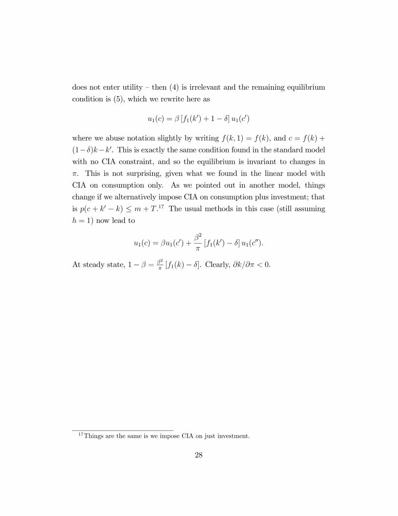
does not enter utility — then (4) is irrelevant and the remaining equilibrium

condition is (5), which we rewrite here as

u1(c) = β [f1(k0) + 1− δ]u1(c

0)

where we abuse notation slightly by writing f(k, 1) = f(k), and c = f(k) +

(1−δ)k−k0. This is exactly the same condition found in the standard modelwith no CIA constraint, and so the equilibrium is invariant to changes in

π. This is not surprising, given what we found in the linear model with

CIA on consumption only. As we pointed out in another model, things

change if we alternatively impose CIA on consumption plus investment; that

is p(c + k0 − k) ≤ m + T .17 The usual methods in this case (still assuming

h = 1) now lead to

u1(c) = βu1(c0) +

β2

π[f1(k

0)− δ]u1(c00).

At steady state, 1− β = β2

π[f1(k)− δ]. Clearly, ∂k/∂π < 0.

17Things are the same is we impose CIA on just investment.

28