Calculation of γ-ray source spectra for used

LWR nuclear fuels

Anastasios Anastasiadis

Supervisor: Peter Andersson Course: Project in Physics and Astronomy, 30.0 c,

1FA193, Master Programme in Nuclear and Particle

Physics, Department of Physics and Astronomy

- 2 -

ABBREVIATIONS

CRAM Chebyshev Rational Approximation Method

CT Cooling Time

LHR Linear Heat Rate

LWR Light Water Reactor

UO2 Uranium dioxide

TRU Transuranic elements

TTA Transmutation Trajectory Analysis

NIST National Institute of Standards and Technology

A Mass number (proton and neutron number)

Eγ γ-ray energy [keV]

kinf Infinite multiplication factor

t1/2 Half-life [s]

Z Atomic number (proton number)

𝜇

𝜌 Mass attenuation coefficient [cm2/g]

ρ Density [g/cm3]

- 3 -

Abstract

The present project aims to provide the γ-ray source spectrum (the

gamma energies and their intensities) for a nuclear fuel, given its

physical dimensions, its enrichment and the detailed knowledge of the

burnup history. In a nuclear reactor, the nuclide concentrations within

the nuclear fuel change due to nuclear transmutation caused by neutron

irradiation and due to the radioactive decay during and after the

irradiation. This alteration in the fuel composition is simulated in this

project with a burnup-mode simulation using the reactor physics code

Serpent 2. A second Serpent 2 photon-mode simulation follows as to

evaluate the γ-radiation spectrum from the respective nuclides produced

in the first simulation. Finally, the γ-ray mass attenuation coefficients

for selected energies are evaluated by combining the fuel elemental

concentrations with the corresponding mass attenuation coefficients for

fresh fuel based on NIST XCOM database. To facilitate the repeated

evaluation of the γ-ray source spectrum, a custom-made MATLAB®

function, GetEmissions, that initiates the Serpent 2 simulations was

created. This function utilizes the user input data, which are the fuel

dimensions, the fuel enrichment and the burnup history, as to

automatically create an input for the Serpent 2 code. Afterwards, it

executes burnup and photon simulations, and finally extracts the data

sought for, which are the emitted by the fuel γ-ray energies and their

intensities (γ-ray source spectrum). In addition, for the given fuel

characteristics, the function provides the mass attenuation coefficient

(𝜇

𝜌) for a selected γ-ray passing the fuel. Using the GetEmissions

function, the gamma spectra from ten nuclear burnup history cases

representing a scan through low and high burnup and short, medium and

long cooling times are calculated. The resulting top ten gamma energies

are listed by absolute intensity, and information about the mother

nuclide and the decay is provided.

- 4 -

Acknowledgements

I would like to thank my supervisor researcher Peter Andersson for the

very useful discussions during our meetings. Peter inspires me

continuously with new ideas and helps me to find the optimum solutions

to go further in research.

I am thankful to the Fission Diagnostics and Safeguards group, Applied

Nuclear Physics division, that gives me the opportunity to participate in

its very useful meeting presentations and discussions.

I also thank the visiting researcher Haluk Atak for the useful

conversations on scientific issues.

I am grateful to the senior lecturer and master studies coordinator

Andreas Korn, who informs me always about the details of my master

studies at Uppsala University.

Finally, I would like to offer my special thanks to the senior lecturer

Matthias Weiszflog for the examination, the careful reading of this

project and the very useful comments.

- 5 -

Table of Contents

1. Introduction ............................................................................................................. - 6 -

2. Theory ...................................................................................................................... - 8 -

2.1 Used fuel parameters ............................................................................................. - 8 -

2.2 γ-radiation and fission products ........................................................................... - 9 -

2.3 Monte Carlo simulations ..................................................................................... - 10 -

3. Modelling and simulations .................................................................................... - 11 -

3.1 GetEmissions function arguments ..................................................................... - 12 -

3.2 Burnup Depletion calculation ............................................................................. - 15 -

3.3 Photon simulation mode ..................................................................................... - 17 -

3.4 Mass Attenuation coefficients function (GetAttenuation.m) ........................... - 18 -

4. Absoulte γ-ray Intensity Results ......................................................................... - 20 -

5. Discussion ............................................................................................................... - 25 -

6. Outlook ................................................................................................................... - 27 -

7. References .............................................................................................................. - 28 -

Appendix .................................................................................................................... - 30 -

- 6 -

1. Introduction

In the nuclear fission diagnostics field, the nuclear fuel behavior can

be investigated by means of non-destructive γ-ray spectroscopic

techniques such as the Gamma Scanning and the Gamma Emission

Tomography. The knowledge of the gamma-emitters distribution in

the fuel, their activity and the γ-rays self-attenuation can help as to

plan irradiation tests at research reactors, in order to optimize

measurement setups and experimental techniques. The current project

belongs to the general framework of the fission diagnostics

performing the diagnosis of the fuel behavior, during irradiation in a

reactor. In this field of study, a widely-used tool for inspection of

nuclear fuel is the γ-ray spectrometry. γ-ray spectrometry is used for

fuel inspections in commercial nuclear power reactors, at interim fuel

storages as well as in research reactors. Radiation detectors can reveal

the pulse-height gamma spectrum of the used fuel rods and the full

energy peak of interest can be extracted as to measure the distribution

of a radionuclide in the rod [1].

Information about the activity of the gamma-emitters in the nuclear

fuel, the γ-rays source energy distribution and the mass attenuation

coefficients for γ-rays passing through the fuel is significant as to plan

irradiation tests for a given instrument at research reactors, predicting

signals and background count rates. It helps also the optimization of

measurement setups in development of future instruments.

During the operation of a reactor, the initial fissile and fertile content

of a nuclear fuel is consumed, and in parallel, new nuclides are

created, such as actinides, fission and activation products. The major

contribution of radioactivity in the first centuries comes from the

fission products. After the neutron irradiation taking place in the

reactor, the used fuel can be removed and be inspected. In that way,

information such as the distribution of a decaying isotope in the fuel

rod and other fuel characteristics like fuel’s burnup and cooling time

- 7 -

(CT) can be provided [2-4]. The characterization of a used fuel can be

useful also for nuclear safeguards and forensic authorities. On one

hand, nuclear safeguards, utilizing tools like gamma tomography, can

verify the presence of used nuclear fuel pins in fuel assemblies at

storage locations, or verify the burnup history of the nuclear fuel [5,

6]. On the other hand, data concerning age dating of nuclear fuels, as

well as a more accurate radionuclides fuel composition knowledge

can be useful for nuclear forensics authorities as to identify criminal

actions [7].

Aiming to provide a predictive tool to be used by practitioners

utilizing γ-ray spectrometry to investigations of high-burnup nuclear

fuels, this project deals with the construction of a modular MATLAB®

function that applies manual or computer-generated input of

fundamental dimensional characteristics of a nuclear fuel, and the

burnup history in any arbitrary level of temporal detail to a predefined

Serpent 2 code [9]. It executes a burnup and a photon simulation based

on the defined input, which includes user-defined information about

the fuel dimensions, enrichment and burnup history. Eventually, it

provides an output of the expected used fuel energy spectrum,

including information about the activity of all radionuclides found in

the reactor, their absolute intensity (photons/sec/cm), the relative

intensity (photons/decay) and their gamma energy lines (keV).

Additionally, for the respective fuel composition it couples other

functions [10] that calculate the mass attenuation coefficient for a

given γ-ray passing through the used fuel.

The performance of the developed MATLAB® function was tested by

examining the existence and disappearance of the short-lived and

long-lived nuclides at different reactor operational and cooling times.

The result was subsequently used to evaluate the dominant γ-ray

intensities and their nuclides of origin, for ten test cases representing

a wide array of nuclear burnups and cooling times.

- 8 -

2. Theory

2.1 Used fuel parameters

Fuel that has been utilized in a reactor is afterwards called irradiated

nuclear fuel. The irradiated nuclear fuel in contrast with the fresh one,

has a complex nuclide composition. In a LWR (Light Water Reactor)

fueled by UO2 (enriched to about 3-5 % uranium-235), the amount of

uranium nuclei is reduced with time either through fission or through

transmutation to heavier actinides and as a result fission products,

minor actinides and TRU (Transuranic elements) appear. When the

fissile material has been decreased to about 0.5 %, the respective fuel

is removed from the reactor’s core and they are stored in an interim

storage for cooling and radiation protection reasons. After that stage,

which can last for decades depending on different reasons such as the

country’s design and construction plans of final repositories, the fuel

can be sealed and be placed under the ground in the repository [4, 10].

However, before coming to that final step of the repository placement,

the fuel can be used for some final inspections. For this reason, there

are some physical quantities that characterize the fuel. For instance,

the enrichment, the burnup, the burnup history, the cooling time (CT)

and the decay heat. The enrichment determines the initial fissile

content (e.g. isotope 235U). The amount of the total thermal energy

production per fuel mass unit is called burnup, while the way it is

distributed in time is the burnup history. The time after the removal

of the rod from the reactor’s core is called cooling time and the heat

produced by the decaying nuclei is called decay heat.

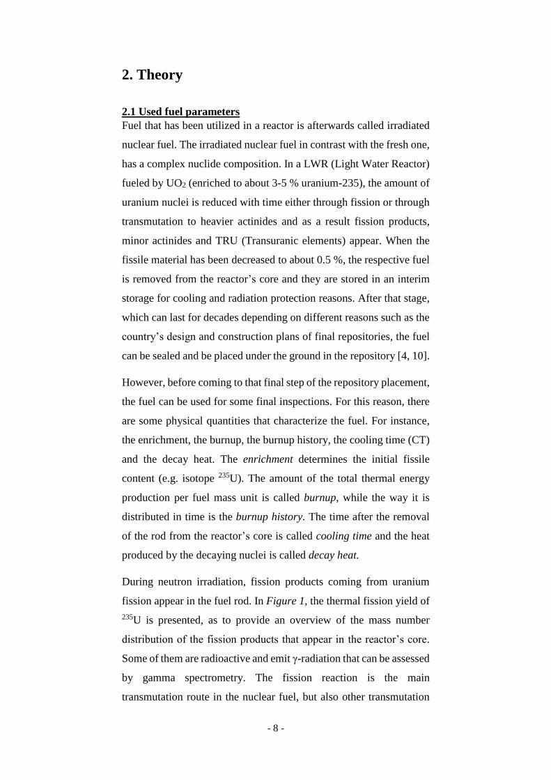
During neutron irradiation, fission products coming from uranium

fission appear in the fuel rod. In Figure 1, the thermal fission yield of

235U is presented, as to provide an overview of the mass number

distribution of the fission products that appear in the reactor’s core.

Some of them are radioactive and emit γ-radiation that can be assessed

by gamma spectrometry. The fission reaction is the main

transmutation route in the nuclear fuel, but also other transmutation

- 9 -

reactions take place, such as neutron capture, and in addition

radioactive decay [11].

2.2 γ-radiation and fission products

The high frequency electromagnetic radiation, γ-radiation, is the

object of study in many nuclear physics areas including both

fundamental and applied nuclear research. In the field of the applied

research, in a reactor the neutron bombardment happens during the

chain reaction and causes transmutation and fission. Many neutron-

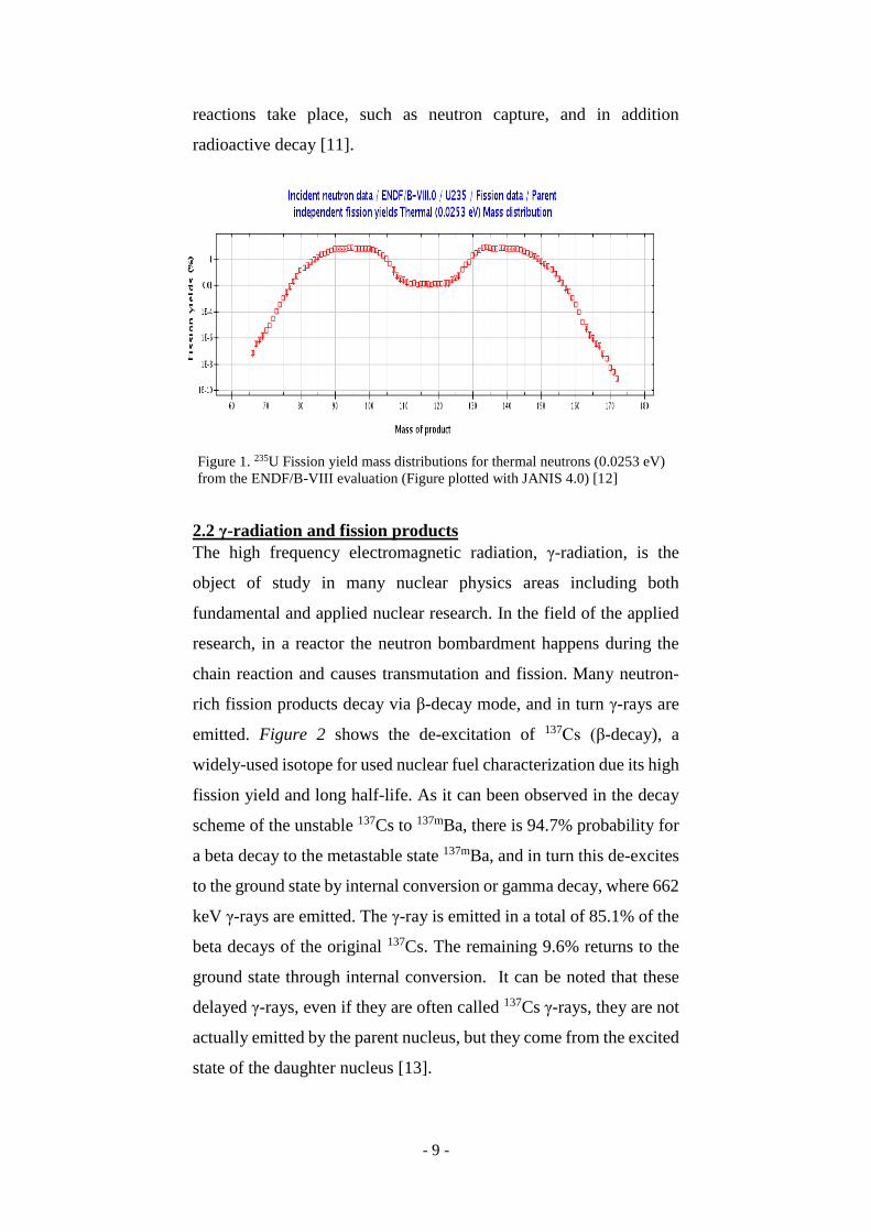
rich fission products decay via β-decay mode, and in turn γ-rays are

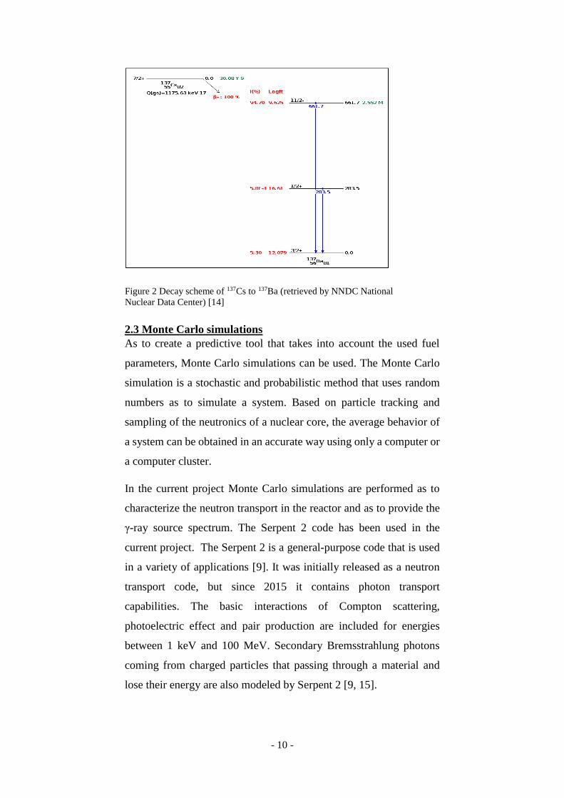
emitted. Figure 2 shows the de-excitation of 137Cs (β-decay), a

widely-used isotope for used nuclear fuel characterization due its high

fission yield and long half-life. As it can been observed in the decay

scheme of the unstable 137Cs to 137mBa, there is 94.7% probability for

a beta decay to the metastable state 137mBa, and in turn this de-excites

to the ground state by internal conversion or gamma decay, where 662

keV γ-rays are emitted. The γ-ray is emitted in a total of 85.1% of the

beta decays of the original 137Cs. The remaining 9.6% returns to the

ground state through internal conversion. It can be noted that these

delayed γ-rays, even if they are often called 137Cs γ-rays, they are not

actually emitted by the parent nucleus, but they come from the excited

state of the daughter nucleus [13].

Figure 1. 235U Fission yield mass distributions for thermal neutrons (0.0253 eV)

from the ENDF/B-VIII evaluation (Figure plotted with JANIS 4.0) [12]

- 10 -

2.3 Monte Carlo simulations

As to create a predictive tool that takes into account the used fuel

parameters, Monte Carlo simulations can be used. The Monte Carlo

simulation is a stochastic and probabilistic method that uses random

numbers as to simulate a system. Based on particle tracking and

sampling of the neutronics of a nuclear core, the average behavior of

a system can be obtained in an accurate way using only a computer or

a computer cluster.

In the current project Monte Carlo simulations are performed as to

characterize the neutron transport in the reactor and as to provide the

γ-ray source spectrum. The Serpent 2 code has been used in the

current project. The Serpent 2 is a general-purpose code that is used

in a variety of applications [9]. It was initially released as a neutron

transport code, but since 2015 it contains photon transport

capabilities. The basic interactions of Compton scattering,

photoelectric effect and pair production are included for energies

between 1 keV and 100 MeV. Secondary Bremsstrahlung photons

coming from charged particles that passing through a material and

lose their energy are also modeled by Serpent 2 [9, 15].

Figure 2 Decay scheme of 137Cs to 137Ba (retrieved by NNDC National

Nuclear Data Center) [14]

- 11 -

3. Modelling and simulations

This project intends to provide a tool for the prediction of the source

spectrum for used UO2 fuels based on the Serpent 2 three-dimensional

continuous energy Monte Carlo Reactor Physics code [9]. For that

purpose, the procedure followed during this project entangles two

Serpent 2 simulations and two MATLAB® functions into one parent

custom-made MATLAB® function called GetEmissions.m.

According to user-defined function arguments that include the fuel

burnup history, enrichment and dimensions, the GetEmissions

function arranges the inserted data into a Serpent 2 burnup simulation

input. Afterwards, the burnup depletion calculation, during which the

decrease of the fuel’s enrichment in parallel with the reactor’s core

energy extraction takes place, is activated. The simulation’s results

are written in a binary restart file as to be used for the photon transport

calculation that follows. The nuclide material compositions turn by a

Serpent 2 internal procedure into elemental compositions, the suitable

photon interaction data are found in the user-given path and the source

is normalized to photon emission rate per cm of fuel rod and gamma

energy. For the execution of the Serpent 2 photon transport

simulation, photon interaction and decay data are used. The photon

interaction data contain information about the Photoelectric effect,

Compton scattering, Rayleigh scattering, pair production and

secondary Bremsstrahlung photons, whereas the decay data include

decay constants, branching ratios, gamma energies and emission

intensities. In case that the photon simulation mode is used only to

evaluate the fuel’s decay after irradiation, the nuclide compositions

are used as to simulate the γ-ray source spectrum. In addition, the

nuclide concentrations created by the burnup depletion calculation

turn externally using MATLAB® functions into elemental

(GetAttenuation.m and xraymu.m [16]) and they are used in

combination with the National Institute of Standards and Technology

- 12 -

(NIST) XCOM database [17] as to calculate the mass attenuation

coefficient ( 𝜇

𝜌 ) of the used fuel for selected energies.

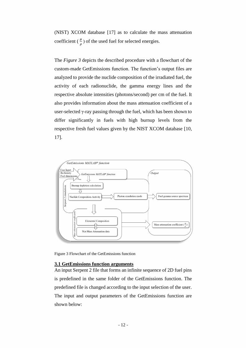
The Figure 3 depicts the described procedure with a flowchart of the

custom-made GetEmissions function. The function’s output files are

analyzed to provide the nuclide composition of the irradiated fuel, the

activity of each radionuclide, the gamma energy lines and the

respective absolute intensities (photons/second) per cm of the fuel. It

also provides information about the mass attenuation coefficient of a

user-selected γ-ray passing through the fuel, which has been shown to

differ significantly in fuels with high burnup levels from the

respective fresh fuel values given by the NIST XCOM database [10,

17].

Figure 3 Flowchart of the GetEmissions function

3.1 GetEmissions function arguments

An input Serpent 2 file that forms an infinite sequence of 2D fuel pins

is predefined in the same folder of the GetEmissions function. The

predefined file is changed according to the input selection of the user.

The input and output parameters of the GetEmissions function are

shown below:

- 13 -

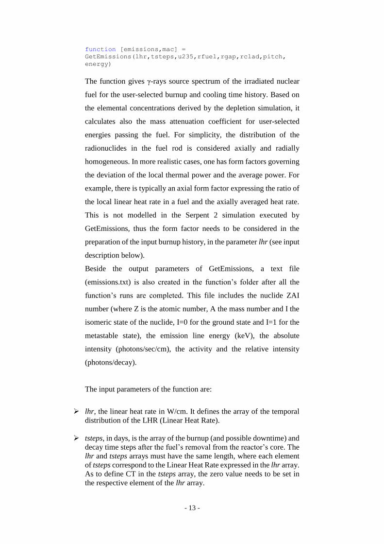
function [emissions,mac] =

GetEmissions(lhr,tsteps,u235,rfuel,rgap,rclad,pitch,

energy)

The function gives γ-rays source spectrum of the irradiated nuclear

fuel for the user-selected burnup and cooling time history. Based on

the elemental concentrations derived by the depletion simulation, it

calculates also the mass attenuation coefficient for user-selected

energies passing the fuel. For simplicity, the distribution of the

radionuclides in the fuel rod is considered axially and radially

homogeneous. In more realistic cases, one has form factors governing

the deviation of the local thermal power and the average power. For

example, there is typically an axial form factor expressing the ratio of

the local linear heat rate in a fuel and the axially averaged heat rate.

This is not modelled in the Serpent 2 simulation executed by

GetEmissions, thus the form factor needs to be considered in the

preparation of the input burnup history, in the parameter lhr (see input

description below).

Beside the output parameters of GetEmissions, a text file

(emissions.txt) is also created in the function’s folder after all the

function’s runs are completed. This file includes the nuclide ZAI

number (where Z is the atomic number, A the mass number and I the

isomeric state of the nuclide, I=0 for the ground state and I=1 for the

metastable state), the emission line energy (keV), the absolute

intensity (photons/sec/cm), the activity and the relative intensity

(photons/decay).

The input parameters of the function are:

➢ lhr, the linear heat rate in W/cm. It defines the array of the temporal

distribution of the LHR (Linear Heat Rate).

➢ tsteps, in days, is the array of the burnup (and possible downtime) and

decay time steps after the fuel’s removal from the reactor’s core. The

lhr and tsteps arrays must have the same length, where each element

of tsteps correspond to the Linear Heat Rate expressed in the lhr array.

As to define CT in the tsteps array, the zero value needs to be set in

the respective element of the lhr array.

- 14 -

➢ u235 is the enrichment of uranium (mass fraction of 235U, between 0

and 1).

➢ rfuel is the radius of the UO2 fuel pins in cm.

➢ rgap is the inner radius of the cladding from the center of the fuel in

cm.

➢ rclad is the outer radius of the cladding (zircalloy is predefined) in cm

➢ pitch defines the distance between the centers of the fuel pins in cm

➢ energy in keV. It defines the γ-ray energy for which the mass

attenuation coefficient is sought for.

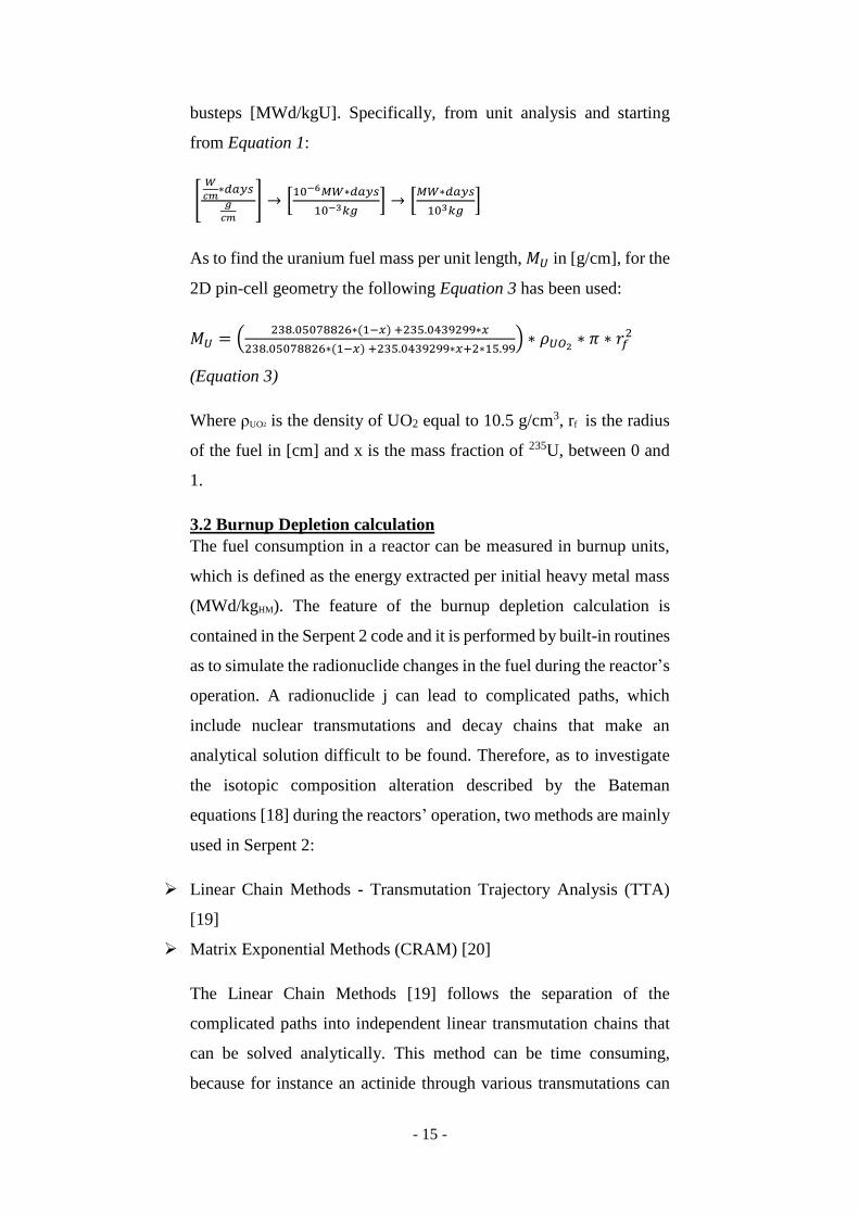
Equation 1 gives the burnup value according to the fuel

characteristics:

𝑏𝑢𝑟𝑛𝑢𝑝 = ∑𝑡𝑖𝑚𝑒(𝑖)∗𝐿𝐻𝑅(𝑖)

𝑚

𝐿 𝑖 (Equation 1)

Where time is given in [days], LHR is the Linear Heat Rate in [W/cm]

and 𝑚

𝐿 is the mass of the uranium fuel per unit length in [g/cm].

According to Equation 1, the GetEmissions code, as to handle

appropriately the Serpent 2 command needs, in terms of time and

burnup units, uses the Equation 2, when the condition of positive lhr

(which for a 2D geometry is defined in [W/cm]) is met. In that way,

the respective data elements defined in the tsteps array are converted

in [MWd/kgU] (busteps). In case of zero lhr element definition in the

lhr array, the respective tsteps array element remain in days. The

busteps represent the elements of the tsteps array when the condition

of the positive lhr is met. They are measured in [MWd/kgU] and they

are described by Equation 2.

𝑏𝑢𝑠𝑡𝑒𝑝𝑠 =𝑡𝑠𝑡𝑒𝑝𝑠∗𝑝𝑜𝑤𝑒𝑟

103∗𝑀𝑈 (Equation 2)

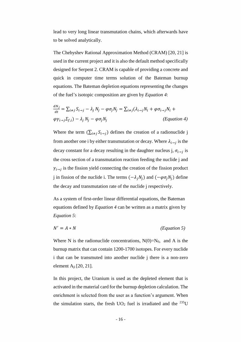
The conversion factor 103 used in Equation 2 is used

programmatically as to convert the tsteps array elements [days] to

- 15 -

busteps [MWd/kgU]. Specifically, from unit analysis and starting

from Equation 1:

[𝑊

𝑐𝑚∗𝑑𝑎𝑦𝑠

𝑔

𝑐𝑚

] → [10−6𝑀𝑊∗𝑑𝑎𝑦𝑠

10−3𝑘𝑔] → [

𝑀𝑊∗𝑑𝑎𝑦𝑠

103𝑘𝑔]

As to find the uranium fuel mass per unit length, 𝑀𝑈 in [g/cm], for the

2D pin-cell geometry the following Equation 3 has been used:

𝑀𝑈 = (238.05078826∗(1−𝑥) +235.0439299∗𝑥

238.05078826∗(1−𝑥) +235.0439299∗𝑥 +2∗15.99

) ∗ 𝜌𝑈𝑂2∗ 𝜋 ∗ 𝑟𝑓

2

(Equation 3)

Where ρUO2 is the density of UO2 equal to 10.5 g/cm3, rf is the radius

of the fuel in [cm] and x is the mass fraction of 235U, between 0 and

1.

3.2 Burnup Depletion calculation

The fuel consumption in a reactor can be measured in burnup units,

which is defined as the energy extracted per initial heavy metal mass

(MWd/kgHM). The feature of the burnup depletion calculation is

contained in the Serpent 2 code and it is performed by built-in routines

as to simulate the radionuclide changes in the fuel during the reactor’s

operation. A radionuclide j can lead to complicated paths, which

include nuclear transmutations and decay chains that make an

analytical solution difficult to be found. Therefore, as to investigate

the isotopic composition alteration described by the Bateman

equations [18] during the reactors’ operation, two methods are mainly

used in Serpent 2:

➢ Linear Chain Methods - Transmutation Trajectory Analysis (TTA)

[19]

➢ Matrix Exponential Methods (CRAM) [20]

The Linear Chain Methods [19] follows the separation of the

complicated paths into independent linear transmutation chains that

can be solved analytically. This method can be time consuming,

because for instance an actinide through various transmutations can

- 16 -

lead to very long linear transmutation chains, which afterwards have

to be solved analytically.

The Chebyshev Rational Approximation Method (CRAM) [20, 21] is

used in the current project and it is also the default method specifically

designed for Serpent 2. CRAM is capable of providing a concrete and

quick in computer time terms solution of the Bateman burnup

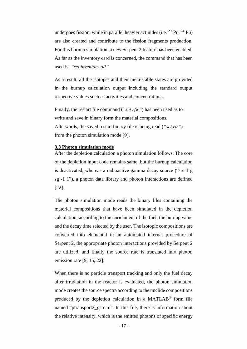
equations. The Bateman depletion equations representing the changes

of the fuel’s isotopic composition are given by Equation 4:

𝑑𝑁𝑗

𝑑𝑡= ∑ 𝑆𝑖→𝑗 − 𝜆𝑗𝑖≠𝑗 𝑁𝑗 − 𝜑𝜎𝑗𝑁𝑗 = ∑ (𝜆𝑖→𝑗𝑁𝑖 + 𝜑𝜎𝑖→𝑗𝑁𝑖 +𝑖≠𝑗

𝜑𝛾𝑖→𝑗𝛴𝑓,𝑖) − 𝜆𝑗 𝑁𝑗 − 𝜑𝜎𝑗𝑁𝑗 (Equation 4)

Where the term (∑ 𝑆𝑖→𝑗)𝑖≠𝑗 defines the creation of a radionuclide j

from another one i by either transmutation or decay. Where 𝜆𝑖→𝑗 is the

decay constant for a decay resulting in the daughter nucleus j, 𝜎𝑖→𝑗 is

the cross section of a transmutation reaction feeding the nuclide j and

𝛾𝑖→𝑗 is the fission yield connecting the creation of the fission product

j in fission of the nuclide i. The terms (−𝜆𝑗𝑁𝑗) and (−𝜑𝜎𝑗𝑁𝑗) define

the decay and transmutation rate of the nuclide j respectively.

As a system of first-order linear differential equations, the Bateman

equations defined by Equation 4 can be written as a matrix given by

Equation 5:

𝑁′ = 𝐴 ∗ 𝑁 (Equation 5)

Where N is the radionuclide concentrations, N(0)=N0, and A is the

burnup matrix that can contain 1200-1700 isotopes. For every nuclide

i that can be transmuted into another nuclide j there is a non-zero

element Aji [20, 21].

In this project, the Uranium is used as the depleted element that is

activated in the material card for the burnup depletion calculation. The

enrichment is selected from the user as a function’s argument. When

the simulation starts, the fresh UO2 fuel is irradiated and the 235U

- 17 -

undergoes fission, while in parallel heavier actinides (i.e. 239Pu, 241Pu)

are also created and contribute to the fission fragments production.

For this burnup simulation, a new Serpent 2 feature has been enabled.

As far as the inventory card is concerned, the command that has been

used is: “set inventory all”

As a result, all the isotopes and their meta-stable states are provided

in the burnup calculation output including the standard output

respective values such as activities and concentrations.

Finally, the restart file command (“set rfw”) has been used as to

write and save in binary form the material compositions.

Afterwards, the saved restart binary file is being read (“set rfr”)

from the photon simulation mode [9].

3.3 Photon simulation mode

After the depletion calculation a photon simulation follows. The core

of the depletion input code remains same, but the burnup calculation

is deactivated, whereas a radioactive gamma decay source (“src 1 g

sg -1 1”), a photon data library and photon interactions are defined

[22].

The photon simulation mode reads the binary files containing the

material compositions that have been simulated in the depletion

calculation, according to the enrichment of the fuel, the burnup value

and the decay time selected by the user. The isotopic compositions are

converted into elemental in an automated internal procedure of

Serpent 2, the appropriate photon interactions provided by Serpent 2

are utilized, and finally the source rate is translated into photon

emission rate [9, 15, 22].

When there is no particle transport tracking and only the fuel decay

after irradiation in the reactor is evaluated, the photon simulation

mode creates the source spectra according to the nuclide compositions

produced by the depletion calculation in a MATLAB® form file

named “ptransport2_gsrc.m”. In this file, there is information about

the relative intensity, which is the emitted photons of specific energy

- 18 -

per decay. In order to obtain the result about the absolute intensity that

refers to the number of photons of a specific energy line emitted per

second (in 2D geometries it is also per cm of the fuel), the

GetEmission.m function multiplies the output of activities given from

the initial neutron transport burnup calculation by the relative

intensity coming from the photon simulation mode. The results are

written in columns and they also provided in an output text file called

“emissions.txt”.

Specifically, this file provides information about each γ-ray energy

emitted from the used nuclear fuel:

• ZAI radionuclide number

• Emission energy line [keV]

• Absolute Intensity [photons/sec/cm]

• Activity [Becquerel/cm]

• Relative Intensity [photons/decay]

3.4 Mass Attenuation coefficients function (GetAttenuation.m)

The NIST XCOM program was used as to obtain the mass attenuation

coefficients [10, 17]. The GetAttenuation.m function was created

based on the xraymu.m MATLAB function [16] and it is coupled in

the GetEmissions.m function as to provide the mass attenuation

coefficient for γ-rays that impinge at the used fuel simulated

according to the user’s input specifications. The xraymu.m function

calculates the data by log-log interpolation of the values provided by

NIST and it handles the discontinuous data in the absorption edges

(K, L, M etc) using the Piecewise Cubic Hermite Interpolating

Polynomial (PCHIP) function (pchip.m). In this project, a modified

version of the xraymu.m function [16] was used as to fit with the

current project purposes. More elements’ mass attenuation coefficient

data was imported to the pre-existing function as to make it able to

handle the heavier actinides. The original xraymu.m function, which

had been built for general purpose x-ray imaging, included mass-

attenuation coefficients for elements up to Z = 94. In addition, the

- 19 -

burnup depletion simulation has been set to provide the isotopic

composition of the fuel. For this reason, all isotopic concentrations

are summed as to be converted into elemental and be used for the mass

attenuation calculation.

According to reference [10] the mass attenuation coefficient values,

provided for fresh fuels by NIST XCOM, are decreased as the burnup

of the fuel increases. The elemental composition of the fuel changes

due to transmutations and fissions. As an outcome, the γ-rays pass

through a fuel composition (including actinides and fission products)

that differs from the initial UO2 fresh fuel. For instance, the gamma

emission energy for 137Cs (Εγ=661.7 keV) experience an average

decrease of the mass attenuation coefficient value of 0.2 % every 5

MWd/kgU for a fuel of UO2 (5% 235U enrichment) [10].

In the low energy region, the photoelectric effect that is strongly

dependent on Z dominates. As the fuel burnup increases, this causes

the depletion of uranium (high atomic number: Z=92) and the parallel

creation of lighter fission products. Consequently, the effective Z

decreases and the photoelectric cross sections is affected, resulting to

the decrease of the mass attenuation coefficients of the γ-rays passing

through a high burnup fuel.

- 20 -

4. Absoulte γ-ray Intensity Results

As to test the capability of the GetEmissions.m function to provide

reasonable results, ten cases were examined. The parameters that have

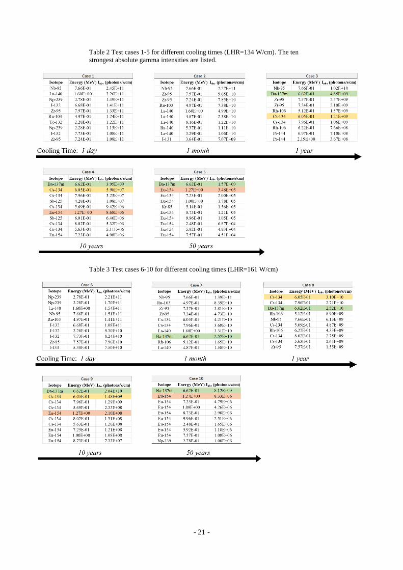
been taken into consideration for all cases are shown in Table 1. For

every single case, is in addition provided a table (Tables 2,3) that

contains information about the ten most intense γ-rays concerning

their absolute intensity [photons/sec/cm] and their energy [keV]. The

LHR was maintained constant during the first five cases at LHR=134

W/cm and during the last five cases it was maintained at LHR= 161

W/cm. In both cases the enrichment was set to 5% of 235U, the radius

of the fuel to 0.410 cm, the inner radius of the cladding to 0.418, the

outer radius of the cladding to 0.475 and the pitch to 1.6 cm.

Table 1. Description of test cases

Analyzing the Tables 2, 3, it can be observed that as the CT increases

there are some radionuclides that dominate the gamma source

spectrum. Some of them have been highlighted and their behavior has

been followed from case to case. As it can been observed, in the long

CT cases (4,5 and 9,10) the 137mBa (which is coming from a beta decay

of 137Cs) dominates. This happens, due to the long half-life of the

mother nuclide 137Cs (30.08 (9) yrs). Except for that, other nuclides

with long half-life such as the 134Cs (t1/2: 2.0652 (4) yrs) and the 154Eu

(t1/2: 8.601 (10) yrs) are also important in the spectra of long-cooled

nuclear fuel.

Cases Burnup (MWd/kgU) Running time (yrs) Cooling time LHGR (W/cm)

1 10 1 1 day 134

2 10 1 1 month 134

3 10 1 1 year 134

4 10 1 10 years 134

5 10 1 50 years 134

6 60 5 1 day 161

7 60 5 1 month 161

8 60 5 1 year 161

9 60 5 10 years 161

10 60 5 50 years 161

- 21 -

Table 2 Test cases 1-5 for different cooling times (LHR=134 W/cm). The ten

strongest absolute gamma intensities are listed.

Table 3 Test cases 6-10 for different cooling times (LHR=161 W/cm)

- 22 -

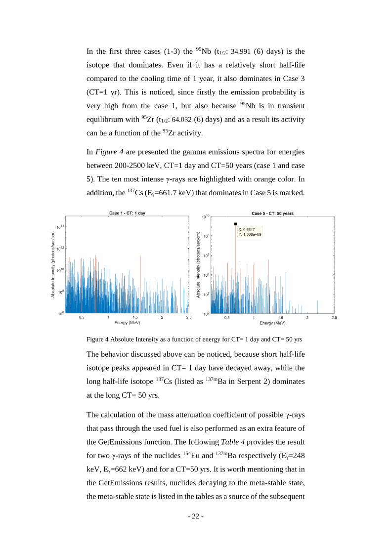
In the first three cases (1-3) the 95Nb (t1/2: 34.991 (6) days) is the

isotope that dominates. Even if it has a relatively short half-life

compared to the cooling time of 1 year, it also dominates in Case 3

(CT=1 yr). This is noticed, since firstly the emission probability is

very high from the case 1, but also because 95Nb is in transient

equilibrium with 95Zr (t1/2: 64.032 (6) days) and as a result its activity

can be a function of the 95Zr activity.

In Figure 4 are presented the gamma emissions spectra for energies

between 200-2500 keV, CT=1 day and CT=50 years (case 1 and case

5). The ten most intense γ-rays are highlighted with orange color. In

addition, the 137Cs (Eγ=661.7 keV) that dominates in Case 5 is marked.

Figure 4 Absolute Intensity as a function of energy for CT= 1 day and CT= 50 yrs

The behavior discussed above can be noticed, because short half-life

isotope peaks appeared in CT= 1 day have decayed away, while the

long half-life isotope 137Cs (listed as 137mBa in Serpent 2) dominates

at the long CT= 50 yrs.

The calculation of the mass attenuation coefficient of possible γ-rays

that pass through the used fuel is also performed as an extra feature of

the GetEmissions function. The following Table 4 provides the result

for two γ-rays of the nuclides 154Eu and 137mBa respectively (Eγ=248

keV, Eγ=662 keV) and for a CT=50 yrs. It is worth mentioning that in

the GetEmissions results, nuclides decaying to the meta-stable state,

the meta-stable state is listed in the tables as a source of the subsequent

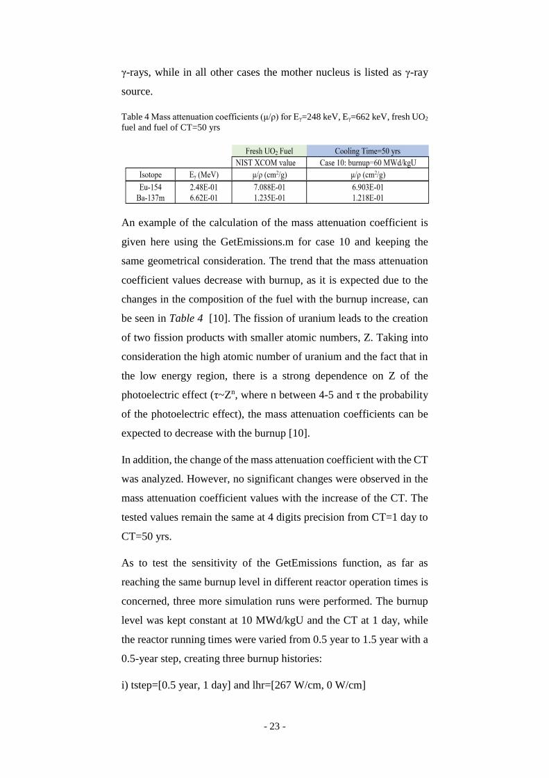
- 23 -

γ-rays, while in all other cases the mother nucleus is listed as γ-ray

source.

Table 4 Mass attenuation coefficients (μ/ρ) for Eγ=248 keV, Eγ=662 keV, fresh UO2

fuel and fuel of CT=50 yrs

An example of the calculation of the mass attenuation coefficient is

given here using the GetEmissions.m for case 10 and keeping the

same geometrical consideration. The trend that the mass attenuation

coefficient values decrease with burnup, as it is expected due to the

changes in the composition of the fuel with the burnup increase, can

be seen in Table 4 [10]. The fission of uranium leads to the creation

of two fission products with smaller atomic numbers, Z. Taking into

consideration the high atomic number of uranium and the fact that in

the low energy region, there is a strong dependence on Z of the

photoelectric effect (τ~Zn, where n between 4-5 and τ the probability

of the photoelectric effect), the mass attenuation coefficients can be

expected to decrease with the burnup [10].

In addition, the change of the mass attenuation coefficient with the CT

was analyzed. However, no significant changes were observed in the

mass attenuation coefficient values with the increase of the CT. The

tested values remain the same at 4 digits precision from CT=1 day to

CT=50 yrs.

As to test the sensitivity of the GetEmissions function, as far as

reaching the same burnup level in different reactor operation times is

concerned, three more simulation runs were performed. The burnup

level was kept constant at 10 MWd/kgU and the CT at 1 day, while

the reactor running times were varied from 0.5 year to 1.5 year with a

0.5-year step, creating three burnup histories:

i) tstep=[0.5 year, 1 day] and lhr=[267 W/cm, 0 W/cm]

- 24 -

ii) tstep=[1 year, 1 day] and lhr=[134 W/cm, 0 W/cm]

iii) tstep=[1.5 year, 1 day] and lhr=[89 W/cm, 0 W/cm]

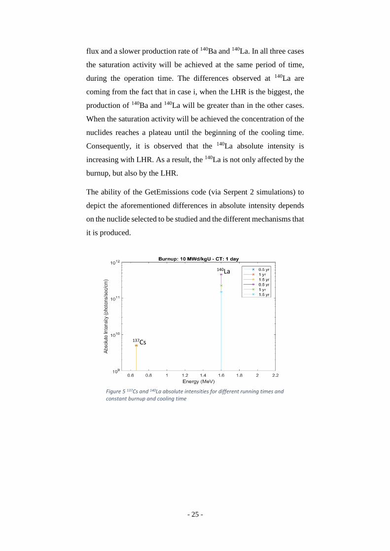
Two radionuclides with different half-life were selected for this study.

The short-lived 140La (t1/2: 1.6781(3) days) and the long-lived 137Cs

(t1/2: 30.08 (9) yrs). Figure 5 shows that the increase of the running

time in general causes the decrease of the absolute intensity of the

gamma emitters found in the reactor’s core. Specifically, the decrease

is bigger for 140La than 137Cs.

From case i to case iii, the running time of the reactor is increased

while the LHR (and the neutron flux) is decreased as to keep the

burnup level constant. On one hand, 137Cs has a long half-life

compared to the running time of the reactor and it does not reach the

saturation activity in any case. For this reason, the 137Cs isotope

concentration is going to be increased continuously during the

reactor’s operation. When the fuel will be removed from the reactor,

the cooling time begins and the concentration of 137Cs will start

decreasing due to the decay process. Consequently, the 137Cs that has

a long half-life compared to the reactor operation time in all three

cases is more depended on the burnup, which is constant here, and not

on the LHR. Eventually, its absolute intensity does not change

significantly in the presented three burnup histories.

On the other hand, 140La has a short half-life. Figure 5 shows bigger

differences for this radionuclide concerning its absolute intensity in

the different reactor running times. 140La concentration is not only

affected by its radioactive decay. It can be not only a fission product,

but also a decay product of 140Ba (t1/2: 12.752 (3) days). It is

approaching transient equilibrium with its mother nucleus, 140Ba, after

a CT of 1 day. Its decay rate is in equilibrium with its creation.

However, both nuclides have short half-lives compared to the running

time of the reactor, and long half-lives compared to the cooling time

of 1 day defined constant in the under examination cases. From case

i) to case iii) the LHR is decreased resulting in a decreased neutron

- 25 -

flux and a slower production rate of 140Ba and 140La. In all three cases

the saturation activity will be achieved at the same period of time,

during the operation time. The differences observed at 140La are

coming from the fact that in case i, when the LHR is the biggest, the

production of 140Ba and 140La will be greater than in the other cases.

When the saturation activity will be achieved the concentration of the

nuclides reaches a plateau until the beginning of the cooling time.

Consequently, it is observed that the 140La absolute intensity is

increasing with LHR. As a result, the 140La is not only affected by the

burnup, but also by the LHR.

The ability of the GetEmissions code (via Serpent 2 simulations) to

depict the aforementioned differences in absolute intensity depends

on the nuclide selected to be studied and the different mechanisms that

it is produced.

137Cs

140La

Figure 5 137Cs and 140La absolute intensities for different running times and constant burnup and cooling time

- 26 -

5. Discussion

In the framework of the current project, a predictive tool

(GetEmissions.m) consisting of custom-made MATLAB® functions

that perform simulations as to predict nuclear fuel parameters of

relevance to γ-ray spectrometry of irradiated nuclear fuel, has been

developed. Specifically, a burnup depletion calculation and a photon

simulation are subsequently performed as to extract information about

the gamma emission probabilities of the fuel’s spectrum. This tool

may be used to provide the gamma source spectrum of a LWR fuel

either using manually provided input fuel parameters and burnup

histories, or using automatically generated input data. The latter

option opens the door for application such as sensitivity analysis of

nuclide activities to parameters such as irradiation time, or for

optimization of test fuel irradiations for creating a desired intensity of

a peak of interest.

The irradiated nuclide composition resulting from the neutron

transport calculation is converted to elemental compositions and is

used for the definition of a radioactive decay source. As a

consequence, the gamma emission probabilities (in photons/sec/cm)

for the defined radioactive source are provided in a text file form, and

as an output parameter of the MATLAB® function, for every γ-

emitting isotope. Additionally, the mass attenuation coefficient for

user-selected γ-ray energy of the irradiated fuel is given as a result.

The GetEmissions.m function includes some basic input arguments

such as the uranium enrichment and the radius of the fuel that can be

defined by the user. However, there is always the option for the user

to interfere in the predefined 2D pin-cell Serpent 2 input geometry

and change the variables of the reactor’s model, in order to further

refine the geometry or the simulation settings. During this project, the

intensities of all nuclides along the fuel’s length have been considered

the same, which is not the case in the reality. In more realistic

representations, due to burnup, swelling, ballooning and the rod’s

- 27 -

position in the assembly, a heterogeneous distribution of the

radionuclides is created [10, 23].

Finally, as to test the operation of the developed function, ten

hypothetical test cases were performed. For these cases, different

burnup histories and CT were tested. The results revealed a reasonable

operation and the long-lived isotopes such as the 137Cs and 154Eu

dominated in long CT, as it was expected. In addition, a sensitivity

analysis was performed concerning the observation of differences

between the absolute intensities of the gamma-emitters that have been

produced at the same burnup level and cooling time, but for different

reactor operation times. It was found that the sensitivity of the

GetEmissions code and the way that the LHR determines the results

change according to the different mechanisms of nuclides’

production.

6. Outlook

Application of the developed prediction tool is foreseen primarily in

the field of nuclear fuel diagnostics, in order to plan test irradiations,

measurement geometries and interrogation times of gamma

spectrometric measurements of nuclear test fuels at research reactors.

As far as to validate the performance of the GetEmissions.m function,

one could benefit greatly from experimental gamma spectra from a

well-characterized setup. In this way, an extra validation of the

predictive capability could be performed.

Furthermore, the methods created in this project are expected to

facilitate the design optimization of a Gamma Emission Tomography

instrument, that is been planned at the division of Applied Nuclear

Physics in Uppsala University.

- 28 -

7. References

[1] Andersson, P., Holcombe, S., Tverberg, T., Inspection of a LOCA Test Rod at

the Halden Reactor Project using Gamma Emission Tomography, Top Fuel 2016 -

LWR Fuels with Enhanced Safety and Performance, American Nuclear Society,

viewed 26 November 2018,

<http://urn.kb.se/resolve?urn=urn:nbn:se:uu:diva-303810>

[2] Holcombe, S., Gamma Spectroscopy and Gamma Emission Tomography for

Fuel Performance Characterization of Irradiated Nuclear Fuel Assemblies, (Ph.D.

thesis), Uppsala Universitet (2014), viewed 16 November 2018,

<http://urn.kb.se/resolve?urn=urn:nbn:se:uu:diva-235124>

[3] Min, D.K., Park H.J., Park, K.J., Ro, S.G., Park, H.S., Determination of burnup,

cooling time and initial enrichment of PWR spent fuel by use of gamma-ray activity

ratios, Proceedings of the Korean Nuclear Society Spring Meeting, Vol. II, Seoul,

Korea, May 1998, p. 545

[4] Davour, A., Svärd, S.J., Andersson, P., Grape, S., Holcombe, S., Jansson, P.,

Troeng, M., Applying image analysis techniques to tomographic images of

irradiated nuclear fuel assemblies, Annals of Nuclear Energy 96, pp 223–229, 2016

[5] Svärd, S.J., Smith, L.E. , White, T.A., Mozin, V., Jansson, P., Andersson, P.,

Davour, A. Grape, S., Trellue, H., Deshmukh, N., Miller, E.A., Wittman, R. S.,

Honkamaa, T., Vaccaro, S., Ely, J., Outcomes of the JNT 1955 Phase I Viability

Study of Gamma Emission Tomography for Spent Fuel Verification, ESARDA

BULLETIN, No. 55, December 2017, viewed 20 November, 2018,

<https://esarda.jrc.ec.europa.eu/images/Bulletin/Files/B_2017_055.pdf>

[6] Willman, C., Håkansson, A., Osifo, O., Bäcklin, A., Svärd, S.J., Nondestructive

assay of spent nuclear fuel with gamma-ray spectroscopy, Annals of Nuclear

Energy, Volume 33, Issue 5, Pages 427-438, 2006

<http://www.sciencedirect.com/science/article/pii/S0306454905002847>

[7] Apostol, A., Pantelica, A., Sima, O., Fugaru, V., Isotopic composition analysis

and age dating of uranium samples by high resolution gamma ray spectrometry,

Nuclear Instruments and Methods in Physics Research, Vol 383, pp.103-108, 2016

[8] MATLAB and Statistics Toolbox Release 2012b, The MathWorks, Inc., Natick,

Massachusetts, United States, 21 September 2017

[9] Leppanen, J., Pusa, M., Viitanen, T., Valtavirta, V., Kaltiaisenaho, T., The

Serpent Monte Carlo code: Status, development and applications in 2013. Ann.

Nucl. Energy, 82, pp 142-150, 2015

[10] Anastasiadis, A., Calculation of γ-ray mass attenuation coefficients (μ/ρ) for

different burnup values of UO2 nuclear fuels in a PWR simulated by Serpent 2

Monte Carlo code, Uppsala University, Applied Nuclear Physics, Independent

thesis Advanced level, 2018, viewed 20 November 2018,

- 29 -

<http://urn.kb.se/resolve?urn=urn:nbn:se:uu:diva-351333>

[11] Willman, C., Applications of Gamma Ray Spectroscopy of Spent Nuclear Fuel

for Safeguards and Encapsulation (PhD dissertation). Acta Universitatis

Upsaliensis, Uppsala, 2016, viewed 1 November

<http://urn.kb.se/resolve?urn=urn:nbn:se:uu:diva-7116>

[12] N. Soppera, M. Bossant, E. Dupont, "JANIS 4: An Improved Version of the

NEA Java-based Nuclear Data Information System", Nuclear Data Sheets, Volume

120, pp 294-296, 2014

[13] Knoll, G. F., Radiation Detection and Measuring, New York: John Wiley &

Sons Inc, pp. 49 to 54, 2000

[14] Kinsey, R. R., et al., The NUDAT/PCNUDAT Program for Nuclear Data, paper

submitted to the 9th International Symposium of Capture Gamma-Ray

Spectroscopy and Related Topics, Budapest, Hungary, October 1996. Data

extracted from the NUDAT database, version Nudat 2, datasheet used: Browne, R.,

Tuli, R. J. K., Nuclear Data Sheets 108, 2173, 2007, viewed 20 November 2018,

<https://www.nndc.bnl.gov/nudat2/chartNuc.jsp>

[15] Kaltiaisenaho, T., Implementing a photon physics model in Serpent 2, M.Sc.

Thesis, Aalto University, 2016.

[16] Errico, J. 2011, A Matlab function to compute the attenuation coefficient,

viewed 22 November 2018,

<http://www.aprendtech.com/blog/Post3/xraymu2.html>

[17] Berger, M.J., Hubbell, J.H., Seltzer, S.M., Chang, J., Coursey, J.S.,

Sukumar, R., Zucker, D.S., and Olsen, K. (2010), XCOM: Photon Cross Section

Database (version 1.5), National Institute of Standards and Technology,

Gaithersburg, MD, viewed 10 November 2018,

<http://physics.nist.gov/xcom>

[18] Bateman, H., The solution of a system of differential equations occurring in the

theory of radioactive transformations, In Proc. Cambridge Philos. Soc Vol. 15, No.

pt V, pp. 423–427, June 1910

[19] Cetnar, J., General solution of Bateman equations for nuclear transmutations,

Annals of Nuclear Energy, Volume 33, Issue 7, Pages 640-645, 2006, viewed 12

November 2018

< http://www.sciencedirect.com/science/article/pii/S0306454906000284>

[20] Pusa M. and Leppänen J., Computing the Matrix Exponential in Burnup

Calculations, Nucl. Sci. Eng., 164, 140-150, 2010

[21] Pusa M. and Leppänen J., An Efficient Implementation of the Chebyshev

Rational Approximation, In. Proc. PHYSOR, 2012

- 30 -

[22] Serpent 2 mediawiki, Radioactive decay source, practical example, viewed 30

October 2018

<http://serpent.vtt.fi/mediawiki/index.php/Radioactive_decay_source,_practical_e

xample>

[23] Schrire, D., Kindlund, A. and Ekberg, P. 1998, Solid Swelling of LWR UO2

fuel, Konferens Halden -98, N(H)-98/10

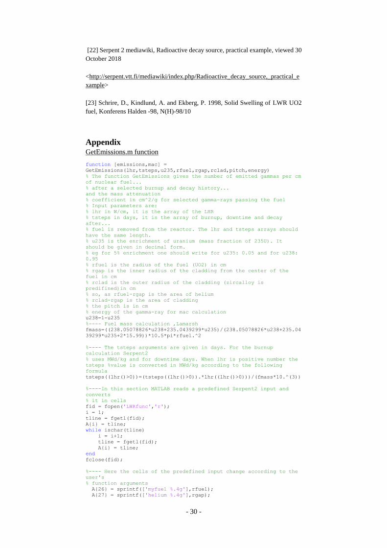
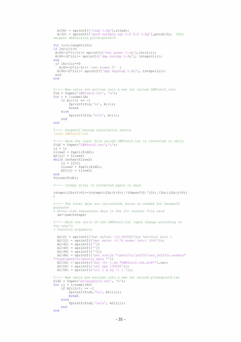
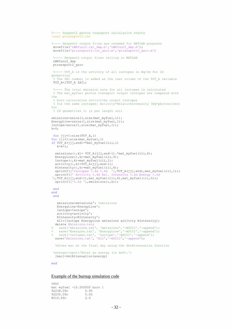
Appendix GetEmissions.m function

function [emissions,mac] =

GetEmissions(lhr,tsteps,u235,rfuel,rgap,rclad,pitch,energy)

% The function GetEmissions gives the number of emitted gammas per cm

of nuclear fuel...

% after a selected burnup and decay history...

and the mass attenuation

% coefficient in cm^2/g for selected gamma-rays passing the fuel

% Input parameters are:

% lhr in W/cm, it is the array of the LHR

% tsteps in days, it is the array of burnup, downtime and decay

after...

% fuel is removed from the reactor. The lhr and tsteps arrays should

have the same length.

% u235 is the enrichment of uranium (mass fraction of 235U). It

should be given in decimal form.

% eg for 5% enrichment one should write for u235: 0.05 and for u238:

0.95

% rfuel is the radius of the fuel (UO2) in cm

% rgap is the inner radius of the cladding from the center of the

fuel in cm

% rclad is the outer radius of the cladding (zircalloy is

predifined)in cm

% so, as rfuel-rgap is the area of helium

% rclad-rgap is the area of cladding

% the pitch is in cm

% energy of the gamma-ray for mac calculation

u238=1-u235

%---- Fuel mass calculation ,Lamarsh

fmass=((238.05078826*u238+235.0439299*u235)/(238.05078826*u238+235.04

39299*u235+2*15.99))*10.5*pi*rfuel.^2

%---- The tsteps arguments are given in days. For the burnup

calculation Serpent2

% uses MWd/kg and for downtime days. When lhr is positive number the

tsteps %value is converted in MWd/kg according to the following

formula

tsteps((lhr()>0))=(tsteps((lhr()>0)).*lhr((lhr()>0)))/(fmass*10.^(3))

%----In this section MATLAB reads a predefined Serpent2 input and

converts

% it in cells

fid = fopen('LWRfunc','r');

i = 1;

tline = fgetl(fid);

A{i} = tline;

while ischar(tline)

i = i+1;

tline = fgetl(fid);

A{i} = tline;

end

fclose(fid);

%---- Here the cells of the predefined input change according to the

user's

% function arguments

A{26} = sprintf(['myfuel %.4g'],rfuel);

A{27} = sprintf(['helium %.4g'],rgap);

- 31 -

A{28} = sprintf(['clad %.4g'],rclad);

A{32} = sprintf(['surf surface sqc 0.0 0.0 %.4g'],pitch/2); %for

serpent definition pitch=pitch/2

for ii=1:length(lhr)

if lhr(ii)>0

A{60+(2*ii-1)}= sprintf(['set power %.4g'],lhr(ii));

A{60+(2*ii)}= sprintf(['dep bustep %.4g'], tsteps(ii));

end

if lhr(ii)==0

A{60+(2*ii-1)}= 'set power 0' ;

A{60+(2*ii)}= sprintf(['dep daystep %.4g'], tsteps(ii));

end

end

%---- New cells are written into a new txt called LWRfunc2.txtc

fid = fopen('LWRfunc2.txt', 'w');

for i = 1:numel(A)

if A{i+1} == -1

fprintf(fid,'%s', A{i});

break

else

fprintf(fid,'%s\n', A{i});

end

end

%---- Serpent2 burnup calculation starts

!sss2 LWRfunc2.txt

%---- Here the input file called LWRfunc2.txt is converted in cells

fid2 = fopen('LWRfunc2.txt','r');

ij = 1;

tline2 = fgetl(fid2);

A2{ij} = tline2;

while ischar(tline2)

ij = ij+1;

tline2 = fgetl(fid2);

A2{ij} = tline2;

end

fclose(fid2);

%---- tsteps array is converted again in days

tsteps((lhr()>0))=(tsteps((lhr()>0)).*(fmass*10.^(3))./lhr((lhr()>0))

)

%---- The total days are calculated, minus is needed for Serpent2

purposes

% minus sign represents days in the rfr restart file card

sa=-sum(tsteps)

%---- Here the cells of the LWRfunc2.txt input change according to

the user's

% function arguments

A2{2} = sprintf(['mat myfuel -10.500000']); %without burn 1

A2{12} = sprintf(['mat water -0.74 moder lwtr1 1001']);

A2{40} = sprintf([''])

A2{44} = sprintf([''])

A2{46} = sprintf(['']);

A2{48} = sprintf(['set acelib "/path/to/jeff31/sss_jeff31u.xsdata"

"/home/path/to/photon_data "'])

A2{54} = sprintf(['set rfr %.4g "LWRfunc2.txt.wrk"'],sa);

A2{56} = sprintf(['set nps 100000']);

A2{58} = sprintf(['src 1 g sg -1 1 ']);

%---- New cells are written into a new txt called ptransport2.txt

fid2 = fopen('ptransport2.txt', 'w');

for ij = 1:numel(A2)

if A2{ij+1} == -1

fprintf(fid2,'%s', A2{ij});

break

else

fprintf(fid2,'%s\n', A2{ij});

end

end

- 32 -

%---- Serpent2 photon transport calculation starts

!sss2 ptransport2.txt

%---- Serpent2 output files are renamed for MATLAB purposes

movefile('LWRfunc2.txt_dep.m','LWRfunc2_dep.m');

movefile('ptransport2.txt_gsrc.m','ptransport2_gsrc.m')

%---- Serpent2 output files calling in MATLAB

LWRfunc2_dep

ptransport2_gsrc

%---- TOT_A is the activity of all isotopes in Bq/cm for 2D

geometries

% The ZAI number is added as the last column of the TOT_A variable

TOT_A=[TOT_A ZAI];

%---- The total emission rate for all isotopes is calculated

% The mat_myfuel photon transport output isotopes are compared with

the

% burn calculation activities output isotopes

% for the same isotopes: Activity*RelativeIntensity (Bq*photons/sec)

for

% 2D geometries it is per length unit

emissions=zeros(1,size(mat_myfuel,1));

EnergyLine=zeros(1,size(mat_myfuel,1));

Isotope=zeros(1,size(mat_myfuel,1));

k=0;

for jjj=1:size(TOT_A,1)

for iii=1:size(mat_myfuel,1)

if TOT_A(jjj,end)==mat_myfuel(iii,1)

k=k+1;

emissions(:,k)= TOT_A(jjj,end-1).*mat_myfuel(iii,6);

EnergyLine(:,k)=mat_myfuel(iii,5);

Isotope(:,k)=mat_myfuel(iii,1);

activity(:,k)=TOT_A(jjj,end-1);

RIntensity(:,k)=mat_myfuel(iii,6);

sprintf(['Isotopes %.4d %.4d '],TOT_A(jjj,end),mat_myfuel(iii,1));

sprintf([' Activity %.4d Rel. Intensity %.4d Energy %.4d

'],TOT_A(jjj,end-1),mat_myfuel(iii,6),mat_myfuel(iii,5));

sprintf(['%.4d '],emissions(:,k));

end

end

end

emissions=emissions'; %emissions

EnergyLine=EnergyLine';

Isotope=Isotope';

activity=activity';

RIntensity=RIntensity';

All=[Isotope EnergyLine emissions activity RIntensity];

delete Emissions.txt;

% save('emissions.txt', 'emissions','-ASCII','-append');

% save('Energies.txt', 'EnergyLine','-ASCII','-append');

% save('Isotopes.txt', 'Isotope','-ASCII','-append');

save('Emissions.txt', 'All','-ASCII','-append');

%Gives mac at the final day using the GetAttenuation function

%energy=input('Enter an energy (in keV):')

[mac]=GetAttenuation(energy)

end

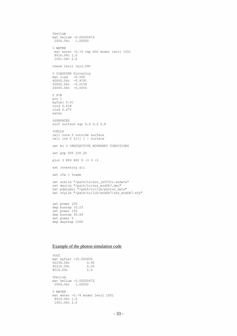
Example of the burnup simulation code

%UO2

mat myfuel -10.500000 burn 1

92238.09c 0.95

92235.09c 0.05

8016.09c 2.0

- 33 -

%helium

mat helium -0.00200472

2004.06c 1.00000

% WATER

mat water -0.74 tmp 600 moder lwtr1 1001

8016.06c 1.0

1001.06c 2.0

therm lwtr1 lwj3.09t

% CLADDING Zircalloy

mat clad -6.560

40000.06c -0.9791

50000.06c -0.0159

26000.06c -0.0050

% PIN

pin 1

myfuel 0.41

void 0.418

clad 0.475

water

%SURFACES

surf surface sqc 0.0 0.0 0.8

%CELLS

cell outw 0 outside surface

cell inw 0 fill 1 - surface

set bc 2 %REFLECTIVE BOUNDARY CONDITIONS

set pop 500 100 20

plot 3 800 800 0 -3 3 -3

set inventory all

set rfw 1 %name

set acelib "/path/to/sss_jeff31u.xsdata"

set declib "/path/to/sss_endfb7.dec"

set pdatadir "/path/to/lib/photon_data"

set nfylib "/path/to/lib/endfb7/sss_endfb7.nfy"

set power 100

dep bustep 10.23

set power 150

dep bustep 30.69

set power 0

dep daystep 1200

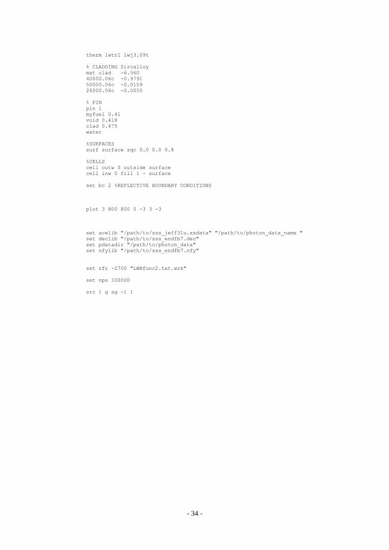
Example of the photon simulation code

%UO2

mat myfuel -10.500000

92238.09c 0.95

92235.09c 0.05

8016.09c 2.0

%helium

mat helium -0.00200472

2004.06c 1.00000

% WATER

mat water -0.74 moder lwtr1 1001

8016.06c 1.0

1001.06c 2.0

- 34 -

therm lwtr1 lwj3.09t

% CLADDING Zircalloy

mat clad -6.560

40000.06c -0.9791

50000.06c -0.0159

26000.06c -0.0050

% PIN

pin 1

myfuel 0.41

void 0.418

clad 0.475

water

%SURFACES

surf surface sqc 0.0 0.0 0.8

%CELLS

cell outw 0 outside surface

cell inw 0 fill 1 - surface

set bc 2 %REFLECTIVE BOUNDARY CONDITIONS

plot 3 800 800 0 -3 3 -3

set acelib "/path/to/sss_jeff31u.xsdata" "/path/to/photon_data_name "

set declib "/path/to/sss_endfb7.dec"

set pdatadir "/path/to/photon_data"

set nfylib "/path/to/sss_endfb7.nfy"

set rfr -2700 "LWRfunc2.txt.wrk"

set nps 100000

src 1 g sg -1 1