arX

iv:h

ep-t

h/93

0909

7v3

5 O

ct 1

993

IASSNS-HEP-93/38CLNS-93/1236

Calabi-Yau Moduli Space, Mirror Manifolds andSpacetime Topology Change in String Theory

Paul S. Aspinwall,† Brian R. Greene♯ and David R. Morrison∗

We analyze the moduli spaces of Calabi-Yau threefolds and their associated confor-

mally invariant nonlinear σ-models and show that they are described by an unexpectedly

rich geometrical structure. Specifically, the Kahler sector of the moduli space of such

Calabi-Yau conformal theories admits a decomposition into adjacent domains some of

which correspond to the (complexified) Kahler cones of topologically distinct manifolds.

These domains are separated by walls corresponding to singular Calabi-Yau spaces in

which the spacetime metric has degenerated in certain regions. We show that the union of

these domains is isomorphic to the complex structure moduli space of a single topological

Calabi-Yau space — the mirror. In this way we resolve a puzzle for mirror symmetry raised

by the apparent asymmetry between the Kahler and complex structure moduli spaces of

a Calabi-Yau manifold. Furthermore, using mirror symmetry, we show that we can inter-

polate in a physically smooth manner between any two theories represented by distinct

points in the Kahler moduli space, even if such points correspond to topologically distinct

spaces. Spacetime topology change in string theory, therefore, is realized by the most basic

operation of deformation by a truly marginal operator. Finally, this work also yields some

important insights on the nature of orbifolds in string theory.

8/93

† School of Natural Sciences, Institute for Advanced Study, Princeton, NJ 08540.♯ F.R. Newman Laboratory of Nuclear Studies, Cornell University, Ithaca, NY 14853.∗ School of Mathematics, Institute for Advanced Study, Princeton, NJ 08540. On leave from:

Department of Mathematics, Duke University, Box 90320, Durham, NC 27708.

1. Introduction

Over the years, research on string theory has followed two main paths. One such path

has been the attempt to extract detailed and specific low energy models from string theory

in an attempt to make contact with observable physics. A wealth of research towards

this end has shown conclusively that string theory contains within it all of the ingredients

essential to building the standard model and that, if we are maximally optimistic about

those things we do not understand at present, fairly realistic low energy models can be

constructed. The second research path has focused on those properties of the theory

which are generic to all models based on strings and which are difficult, if not impossible, to

accommodate in a theory based on point particles. Such properties single out characteristic

“stringy” phenomena and hence constitute the true distinguishing features of string theory.

With our present inability to extract definitive low energy predictions from string theory,

there is strong motivation to study these generic features.

One such feature was identified some time ago in the work of [1]. These authors

showed that whereas point particle theories appear to require a smooth background space-

time, string theory is well defined in the presence of a certain class of spacetime singu-

larities: toroidal quotient singularities. Another characteristically stringy feature is that

of mirror symmetry and mirror manifolds. Mirror symmetry was conjectured based upon

naturality arguments in [2,3], was strongly suggested by the computer studies of [4], and

was established to exist in certain cases by direct construction in [5]. The phenomenon

of mirror manifolds shows that vastly different spacetime backgrounds can give rise to

identical physics — something quite unexpected in nonstring based theories such as gen-

eral relativity and Kaluza-Klein theory. The present work is a natural progression along

these lines of research. By using mirror symmetry we show, amongst other things, that

the topology of spacetime can change by passing through a mathematically singular space

while the physics of string theory is perfectly well behaved.

From a more general vantage point, the present work focuses on the structure of the

moduli spaces of Calabi-Yau manifolds and their associated superconformal nonlinear σ-

models. There has been much work on this subject over the last few years [6], mainly

focusing on local properties. The burden of the sequel is to show that an investigation of

more global properties reveals a remarkably rich structure. As we shall see, whereas previ-

ous studies [6] have, as a prime example, considered the local geometry of the complexified

Kahler cone for a Calabi-Yau space of a fixed topology, we find that a more global perspec-

tive shows that numerous such Kahler cones for topologically distinct Calabi-Yau spaces

1

(and other more exotic entities to be discussed) fit together by adjoining along common

walls to form what we term the enlarged Kahler moduli space. The common walls of these

Kahler cones correspond to metrically degenerate Calabi-Yau spaces in which some homo-

logically nontrivial cycle has zero volume. In other words, points in these walls correspond

to a configuration in which some nontrivial subvariety of the Calabi-Yau space (or, in fact,

the whole Calabi-Yau itself!) is shrunk down to a point. Nonetheless, we show, by making

use of mirror symmetry, that a generic point in such a wall corresponds to a perfectly well

behaved conformal field theory. In fact, the generic point in such a wall has no special

significance from the point of view of conformal field theory and hence none from the point

of view of physics. As is familiar from previous studies, one can move around a path in

moduli space by changing the expectation value of truly marginal operators. We show

that a typical path passes through these walls without any unusual physical consequence.

Hence, this makes it evident that it is physically incomplete to study a single Kahler cone.

There are four main implications of this newfound need to pass from a single com-

plexified Kahler cone to the enlarged Kahler moduli space:

1) Mirror symmetry, combined with standard reasoning from conformal field theory,

leads one to the conclusion that if X and Y are a mirror pair of Calabi-Yau spaces then

the complexified Kahler moduli space of X is isomorphic to the complex structure moduli

space of Y and vice versa [5]. This is a puzzling statement mathematically because a

complexified Kahler moduli space is a bounded domain (as we shall discuss this is due

to the usual constraints that the Kahler form should yield positive volumes) whereas a

complex structure moduli space is not bounded, but is rather of the form A − B with A

and B subvarieties of some projective space [7]. The present work shows that the true

object which is mirror to a complex structure moduli space is not a single complexified

Kahler cone, but rather the enlarged Kahler moduli space introduced above. We show that

the latter has an identical mathematical description (using toric geometry) as the mirror’s

complex structure moduli space, thus resolving this important issue.

2) In the example considered in [8] and discussed in greater detail here, the enlarged

Kahler moduli space consists of 100 distinct regions. In the more familiar example of the

mirror of the quintic hypersurface, we expect the number of regions in the enlarged Kahler

moduli space to be far greater – possibly many orders of magnitude greater – than in the

example studied here. An important question is to give the physical interpretation of the

theories in each region. In [8] we found that five of the 100 regions in our example were

2

interpretable as the complexified Kahler moduli spaces of five topologically distinct Calabi-

Yau spaces related by the operation of flopping [9,10]. We will review this shortly. What

about the other 95 regions? We will postpone a detailed answer to this question to section

VI and also to a forthcoming paper, but there is one essential point worthy of emphasis

here. Some of these regions correspond to Calabi-Yau spaces with orbifold singularities

(similar to those studied in [1] except that the covering space is a nontoroidal Calabi-Yau

space). Conventional wisdom and detailed analyses have always considered such orbifolds

to be “boundary points in Calabi-Yau moduli space”. This implies, in particular, that

smooth Calabi-Yau theories are represented by the generic points in moduli space while

orbifold theories are special isolated points. It also implies that by giving any nonzero

expectation value to “blow-up modes” in the orbifold theory, we move from the orbifold

theory to a smooth Calabi-Yau theory. The present work shows that these interpretations

of the orbifold results are misleading. Rather, it is better to think of orbifold theories

as occupying their own regions in the enlarged Kahler moduli space and hence they are

just as generic as smooth Calabi-Yau theories, which simply correspond to other regions.

Furthermore, these orbifold regions are adjacent to smooth Calabi-Yau regions, but turning

on expectation values for twist fields does not immediately resolve the singularities and

move one into the Calabi-Yau region. Rather, one must traverse the orbifold region by

turning on an expectation value for a twist field until one reaches a wall of the smooth

Calabi-Yau region. Then, if one goes further (for which there is no physical obstruction)

one enters the region of smooth Calabi-Yau theories. This is a significant departure from

the hitherto espoused description of orbifolds in string theory.

3) In the mirror manifold construction of [5], typically both the original Calabi-Yau

space and its mirror are singular. Quite generally, there is more than one way of repairing

these singularities to yield a smooth Calabi-Yau manifold, and the resulting smooth spaces

can be topologically distinct. A natural question is: is one or some subset of these possible

desingularizations (which are on equal footing mathematically) singled out by string theory,

or are all possible desingularizations realized by physical models? We show that each

possible desingularization to a smooth Calabi-Yau manifold has its own region in the fully

enlarged Kahler moduli space. (In fact, these particular regions constitute what we call

the partially enlarged Kahler moduli space.)

4) As remarked earlier, and as will be one of our main foci, the present work estab-

lishes the veracity of the long suspected belief that string theory admits physically smooth

processes which can result in a change of the topology of spacetime. Some of the regions

3

in the enlarged Kahler moduli space correspond to the complexified Kahler cones of topo-

logically distinct smooth Calabi-Yau manifolds. Since we show that there is no physical

obstruction to deforming our theories by truly marginal operators which take us smoothly

from one region to another, we see that we can change the topology of spacetime in a

physically smooth manner. Furthermore, there is nothing at all exotic about such pro-

cesses. They correspond to the most basic kind of deformation to which one can subject a

conformal field theory. This should be contrasted to the situation where one can change

the topology of a Calabi-Yau manifold by passing through a conifold point in the moduli

space as studied in [11]. In such a process one necessarily encounters singularities.

Our approach to establishing these results [8], as mentioned, relies heavily on prop-

erties of mirror manifolds originally established in [5]. These will be reviewed in the next

section. Basically, mirror symmetry has established that a given conformal field theory

may have more than one geometrical realization as a nonlinear σ-model with a Calabi-Yau

target space. Two totally different Calabi-Yau spaces can give rise to isomorphic confor-

mal theories (with the isomorphism being given by a change of sign of a certain charge).

One important implication of this result is that any physical observable in the underlying

conformal theory has two geometrical interpretations — one on each of the associated

Calabi-Yau spaces. Furthermore, a one parameter family of conformal field theories of

this sort likewise has two geometrical interpretations in terms of a family of Calabi-Yau

spaces and in terms of a mirror family of Calabi-Yau spaces. The mirror manifold phe-

nomenon can be an extremely powerful physical tool because certain questions which are

hard to analyze in one geometrical interpretation are far easier to address on the mirror.

For instance, as shown in [5], certain observables which have an extremely complicated

geometrical realization on one of the Calabi-Yau spaces (involving an infinite series of in-

stanton corrections, for example) have an equally simple geometrical interpretation on the

mirror Calabi-Yau space (involving a single calculable integral over the space).

For the question of topology change, and more generally, the question of the struc-

ture of Calabi-Yau moduli space, we make use of mirror manifolds in the following way.

The picture we are presenting implies that under mirror symmetry the complex structure

moduli space of Y is mapped to the enlarged Kahler moduli space of X (and vice versa).

From this we conclude that for any point in the enlarged Kahler moduli space of X we can

find a corresponding point in the complex structure moduli space of Y such that correla-

tion functions of corresponding observables are identically equal since these points should

correspond to isomorphic conformal theories. By choosing representative points which lie

4

in distinct regions of the enlarged Kahler moduli space of X , the veracity of the latter

statement provides an extremely sensitive test of the picture we are presenting. In [8]

as amplified upon here, we showed that this prediction could be explicitly verified in a

nontrivial example.

The picture of topology change, therefore, as discussed in [8] and here can be sum-

marized as follows. We consider a one parameter family of conformal field theories which

have a mirror manifold realization. On one of these two families of Calabi-Yau spaces, the

topological type changes as we progress through the family since we pass through a wall in

the enlarged Kahler moduli space. Classically one would expect to encounter a singularity

in this process. However, although the classical geometry passes through a singularity, it

is possible that the quantum physics does not1. This is a difficult possibility to analyze

directly because it is precisely in this circumstance — one in which the volume of curves in

the internal space are small — that we do not trust perturbative methods in quantum field

theory. However, it proves extremely worthwhile to consider the description on the mirror

family of Calabi-Yau spaces. On the mirror family, only the complex structure changes

and the Kahler form can be fixed at a large value, thereby allowing perturbation theory to

be reliable. As we shall discuss, on the mirror family no topology change occurs — rather

a continuous change of shape accompanied by smoothly varying physical observables is all

that transpires. Thus, on the mirror family we can directly see that no physical singularity

is encountered even though one of our geometrical descriptions involves a discontinuous

change in topology2.

1 We emphasize that all of our analysis is at string tree-level and our use of the term “quantum”

throughout this paper refers to quantum properties of the two-dimensional conformal field theory

on the sphere which describes classical string propagation. It might be more precise to use the

word “stringy” instead of “quantum” but we shall continue to use the latter common parlance.2 One might interpret this statement to mean that — at some level — no topology change

is really occurring so long as one makes use of the correct geometrical description. This is not

true. A more precise version of the statement given in the text, and one which will be explained

fully in the sequel, is: certain topology changing transitions associated with changing the Kahler

structure on a Calabi-Yau space can be reformulated as physically smooth topology preserving

deformations of the complex structure on its mirror. The general situation is one in which the

Kahler structure and the complex structure of a given Calabi-Yau change and hence similarly for

its mirror. Generically, the Kahler structure deformations of both the original Calabi-Yau and

its mirror will result in both families undergoing topology change. We can analyze the physical

description of such transitions by studying the mirror equivalent complex structure deformations

5

To avoid confusion, we emphasize that the topology changing transitions which we

study are not between a Calabi-Yau and its mirror. Rather, mirror manifolds are used as a

tool to study topology changing transitions in which, for example, the Hodge numbers are

preserved and only more subtle topological invariants change. The observation that a given

Calabi-Yau space may have a number of “close relatives” with the same Hodge numbers

but a different topology (constructed by flopping) was made a number of years ago by Tian

and Yau [9]. What is new here is the smooth interpolation between the σ-models based

on these different spaces.

Although this picture of topology change, as presented and verified in [8], is both

compelling and convincing, it is natural to wonder how string theory, at a microscopic level,

avoids a physical singularity when passing through a topology changing transition. The

local description of the topology changing transitions studied here was given in [12] which,

contemporaneously with [8], established this first concrete arena of spacetime topology

change. In [12], by direct examination of particular correlation functions it was shown that

quantum corrections exactly cancel the discontinuity that is experienced by the classical

contribution — in precise agreement with what is expected based on [8]. Moreover, the

results of [12] thoroughly and precisely map out the physical significance of regions in

the “fully enlarged Kahler moduli space” (which we shall discuss in some detail). These

regions are interpreted in [12] as phases of N = 2 quantum field theories and shown to

include Calabi-Yau σ-models on birationally equivalent but topologically distinct target

spaces, Landau-Ginzburg theories and other “hybrid” models which we shall discuss in

section VI. The results of [12] have helped to shape the interpretations we give here and

provide complimentary evidence in support of the topology changing processes we present.

Much of this paper is aimed at explaining the methods and results of [8]. In section

II we will give a more detailed summary of the topology changing picture established in

[8] while emphasizing the background material on mirror manifolds that is required. We

will see that our discussion requires some understanding of toric geometry and we will

give a detailed primer on this subject in section III. In section IV we shall apply some

concepts of toric geometry to discuss mirror symmetry following [13] and [14]. We will

extend this discussion to yield a toric description of the Kahler and complex structure

moduli spaces — naturally leading to the important concepts of the secondary fan , the

(and hence see that the physical description is smooth) but we cannot give a nonlinear σ-model

geometrical interpretation which does not involve topology change.

6

“partially” enlarged Kahler moduli space and the monomial-divisor mirror map. In section

V we shall apply these concepts to verify our picture of moduli space, the action of mirror

symmetry and topology change. We will do this in the context of a particularly tractable

example, but it will be clear that our results are general. We will review the calculation

of [8] which established the topology changing picture reviewed above. In section VI we

will indicate the structure of the “fully” enlarged moduli space alluded to above and in [8],

and show its relation to the “hybrid” models found in [12]. We will leave some important

calculations in these theories to a forthcoming paper. Finally, in section VII we shall offer

our conclusions.

2. Mirror Manifolds, Moduli Spaces and Topology Change

In this section we aim to give an overview of the topology changing picture established

in [8] and use subsequent sections to fill in essential technical details that shall arise in our

discussion.

2.1. Mirror Manifolds

Mirror symmetry was conjectured based upon naturality arguments in [2,3], was sug-

gested by the computer studies of [4] and was established to exist in certain cases by

direction construction in [5]. Mirror symmetry describes a situation in which two very

different Calabi-Yau spaces (of the same complex dimension) X and Y , when taken as

target spaces for two-dimensional nonlinear σ-models, give rise to isomorphic N = 2 su-

perconformal field theories (with the explicit isomorphism involving a change in the sign of

a certain U(1) charge). Such a pair of Calabi-Yau spaces X and Y are said to constitute a

mirror pair [5]. Note that the tree level actions of these σ-models are thoroughly different

as X and Y are topologically distinct. Nonetheless, when each such action is modified by

the series of corrections required by quantum mechanical conformal invariance, the two

nonlinear σ-models become isomorphic.

The naturality arguments of [2,3] were based on the observation that the two types

of moduli in a Calabi-Yau σ-model — the Kahler and complex structure moduli (see

the following subsections for a brief review) — are very different geometrical objects.

However, their conformal field theory counterparts — truly marginal operators — differ

only by the sign of their charge under a U(1) subgroup of the superconformal algebra. It is

unnatural that a pronounced geometric distinction corresponds to such a minor conformal

7

field theory distinction. This unnatural circumstance would be resolved if for each such

conformal theory there is a second Calabi-Yau space interpretation in which the association

of conformal fields and geometrical moduli is reversed (with respect to this U(1) charge)

relative to the first. If this scenario were to be realized, it would imply, for instance, the

existence of pairs of Calabi-Yau spaces whose Hodge numbers satisfy hp,qX = hd−p,q

Y . A

computer survey of hypersurfaces for the case d = 3 [4] revealed a host of such pairs. It is

important to realize, especially in light of more recent mathematical discussions of mirror

symmetry [13,14], that if X and Y satisfy the appropriate Hodge number identity this by

no means establishes that they form a mirror pair. To be a mirror pair, X and Y must

correspond to the same conformal field theory. Such mirror pairs of Calabi-Yau spaces

were constructed in [5] and at present are the only known examples of mirror manifolds.

This construction will play a central role in our analysis so we now briefly review it.

In [5] it was shown that any string vacuum K built from products of N = 2 minimal

models [15] respects a certain symmetry group G such that K and K/G are isomorphic

conformal theories with the explicit isomorphism being given by a change in sign of the left

moving U(1) quantum numbers of all conformal fields. Furthermore, G has a geometrical

interpretation [5] as an action on the Calabi-Yau space X0 associated to K [16,17]. This

geometrical action, in contrast to its conformal field theory realization, does not yield

an isomorphic Calabi-Yau space. Rather, X0 and Y0 = X0/G are topologically quite

different. Nonetheless, K and K/G are geometrically interpretable in terms of X0 and

Y0, respectively — and since the former are isomorphic conformal theories, the latter

topologically distinct Calabi-Yau spaces yield isomorphic nonlinear σ-models3. The two

Calabi-Yau spaces therefore constitute a mirror pair. As we will discuss in more detail

below, the explicit isomorphism between K and K/G being a reversal of the sign of the

left moving U(1) charge implies that X0 and Y0 have Hodge numbers (when singularities

are suitably resolved) which satisfy the mirror relation given in the last paragraph.

Having built a specific mirror pair of theories, as stressed in [5], one can now use

marginal operators to move about the moduli space of each theory to construct whole

3 In light of the results of [12] which reveal a subtlety in the Calabi-Yau/Landau-Ginzburg

correspondence, the arguments of [5] more precisely show that the Landau-Ginzburg (orbifold)

theory corresponding to K and that associated to K/G are isomorphic. To arrive at the geometric

correspondence between X0 and Y0, one must vary the parameters in the theory. This point should

become clear in section VI.

8

families of mirror pairs. It is important to realize however that this process is being per-

formed at the level of conformal field theory and that there may be some subtle difficulties

in translating this into statements about the geometry of mirror families. In fact, it was

shown in [18] that there is an apparent contradiction between the structure of the moduli

space of Kahler forms according to classical geometry and according to conformal field

theory. This issue thus carries into mirror symmetry [19]. If one builds a mirror pair of

theories by the method of [5], then at least one theory will be an orbifold and the as-

sociated target space will have quotient singularities. Classically, varying parameters in

the local moduli space of Kahler forms around this point has the effect of “blowing-up”

these singularities. Typically this process is not unique and so leads to a fan-like structure

with many regions as will be discussed. Such a structure is not seen locally in the mirror

partner. It was suggested in [19] that a resolution of this conundrum would occur if string

theory were somehow able to smooth out so-called “flops” which relate different blow-ups

to each other. In this paper we will describe exactly how to to study the geometry of

mirror families. We will see how the fan-like structure appears the moduli space of con-

formal field theories once one looks at the global structure of the moduli space and that

flop transitions are indeed smoothed out in string theory. We will also find that there are

many other transitions that can occur in the fan structure.

2.2. Conformal Field Theory Moduli Space

Amongst the operators which belong to a given conformal field theory there is a special

subset, {Φi}, consisting of “truly marginal operators”. These operators have the property

that they have conformal dimension (1, 1) and hence can be used to deform the original

theory through the addition of terms to the original action which to first order have the

form ∑ti

∫d2zΦi. (2.1)

The Φi being truly marginal, higher order terms can be chosen so that the resulting theory

is still conformal. We consider all such theories that can be constructed in this manner to

be in the same family — differing from each other by truly marginal perturbations. The

parameter space of all such conformal field theories is known as the moduli space of the

family.

If we consider a family of conformal field theories which have a geometrical interpre-

tation in terms of a family of nonlinear σ-models, we can give a geometrical interpretation

9

to the conformal field theory moduli space. Namely, marginal perturbations in confor-

mal field theory correspond to deformations of the target space geometry which preserve

conformal invariance. In the case of interest to us, we study N = 2 superconformal field

theories which correspond to nonlinear σ-models with Calabi-Yau target spaces. We will

also impose the condition that the Hodge number h2,0 = 0. There are two types of geo-

metrical deformations of these spaces which preserve the Calabi-Yau condition and hence

do not spoil conformal invariance. Namely, one can deform the complex structure or one

can deform the Kahler structure. In fact, with the above condition on h2,0, all of the

truly marginal operators Φi appearing in (2.1) have a geometric realization in terms of

complex structure and Kahler structure moduli of the associated Calabi-Yau space, and

these two sectors are independent of each other. The conformal field theory moduli space

is therefore geometrically interpretable in terms of the moduli spaces parametrizing all

possible complex and Kahler structure deformations of the associated Calabi-Yau space,

and is locally a product of the moduli space of complex structures and the moduli space

of Kahler structures.

The truly marginal operators Φi are endowed with an additional quantum number:

their charge under a U(1) subgroup of the N = 2 superconformal algebra. This charge can

be 1 or −1 and hence the set of all Φi can partitioned into two sets according to the sign

of this quantum number. One such set corresponds to the Kahler moduli of X and the

other set corresponds to the complex structure moduli of X . It is rather unnatural that

such a trivial conformal field theory distinction — the sign of a U(1) charge — has such

a pronounced geometrical interpretation. The mirror manifold scenario removes this issue

in that if Y is the mirror of X then the association of truly marginal conformal fields to

geometrical moduli is reversed relative to X . In this way, each truly marginal operator has

an interpretation as both a Kahler and a complex structure moduli — albeit on distinct

spaces.

In the next two subsections we shall describe the two geometrical moduli spaces—

the spaces of complex structures and of Kahler structures—in turn. Our discussion will,

for the most part, be a classical mathematical exposition of these moduli spaces. It is

important to realize that classical mathematical formulations are generally lowest order

approximations to structures in conformal field theory. The description of the Kahler

moduli space given below most certainly is only a classical approximation to the structure of

the corresponding quantum conformal field theory moduli space. An important implication

of this for our purposes is that if our classical analysis indicates that a point in the Kahler

10

moduli space corresponds to a singular Calabi-Yau space, it does not necessarily follow

that the associated conformal field theory is singular (i.e. has badly behaved physical

observables). Physical properties and geometrical properties are related but they are not

identical. One might think that a similar statement could be made regarding the complex

structure moduli space — however in our applications there is a crucial difference. We will

only need to study the physical properties of theories represented by points in the complex

structure moduli space which correspond to smooth (i.e. transverse) complex structures.

By Yau’s theorem [20], in such a circumstance, one can find a smooth Ricci-flat metric

(which solves the lowest order β-function equations) which is in the same cohomology class

as any chosen Kahler form on the manifold. By choosing this Kahler form to be “large”

(large overall volume and large volume for all rational curves) we can trust perturbation

theory and all physical observables are perfectly well defined. Thus, we can trust that

nonsingular points in the complex structure moduli space give rise to nonsingular physics

(for sufficiently general choices of the Kahler class). It is this fact which shall play a crucial

role in our analysis of topology changing transitions.

2.3. Complex Structure Moduli Space

A given real 2d dimensional manifold may admit more than one way of being viewed

as a complex d dimensional manifold. Concretely, a complex d-dimensional manifold is

one in which complex coordinates z1, . . . , zd have been specified in various “coordinate

patches” such that transition functions between patches are holomorphic functions of these

coordinates. Any two sets of such complex coordinates which themselves differ by an

invertible holomorphic change of variables are considered equivalent. If there is no such

holomorphic change of variables between two sets of complex coordinates, they are said to

define different complex structures on the underlying real manifold.

Given a complex structure on a complex manifold X , there is a cohomology group

which parameterizes all possible infinitesimal deformations of the complex structure:

H1(X, T ), where T is the holomorphic tangent bundle. For the case ofX being Calabi-Yau,

it has been shown [21] that there is no obstruction to integrating infinitesimal deforma-

tions to finite deformations and hence this cohomology group may be taken as the tangent

space to the parameter space of all possible complex structures on X . As is well known,

because X has a nowhere vanishing holomorphic (d, 0) form, we have the isomorphism

H1(X, T ) ∼= Hd−1,1(X). For certain types of Calabi-Yau spaces X , there is a simple way

11

of describing these complex structures. In the present paper we will focus almost exclu-

sively on hypersurfaces in weighted projective space. So, let X be given as the vanishing

locus of a single homogeneous polynomial in the weighted projective space P(d+1){k0....,kd}

. Our

notation here is that if z0., . . . , zd are homogeneous coordinates in this weighted projective

space then we have the identification

[z0., . . . , zd] ∼= [λk0z0, . . . , λkdzd]. (2.2)

For X to be Calabi-Yau it must be homogeneous of degree equal to the sum of the weights

ki. Consider the most general form for the defining equation of X

W =∑

ai0i1...idzp0

i0. . . zpd

id= 0 (2.3)

with∑kijpj =

∑kj. In order to count each complex structure that arises here only

once, we must make identifications among sets of coefficients ai0i1...idwhich give rise to

isomorphic hypersurfaces through general projective linear coordinate transformations on

the zi. This gives a space of possible complex structures that can be put on the real

manifold underlying X (but in general there may be other complex structures as well

[22]). Thus, we have a very simple description of this part of the complex structure moduli

space of the Calabi-Yau manifold X . We will illustrate these ideas in an explicit example

in section V.

Given a Calabi-Yau hypersurface defined by (2.3), note that each monomial zp0

i0. . . zpd

id

appearing in (2.3) can be regarded as a truly marginal operator which deforms the complex

structure. These deformations enter into (2.3) in a purely linear way—no higher order

corrections are necessary.

One subtlety in the above description is that not all choices of the coefficients ai0i1...id

lead to a nonsingular X .4 Namely, if there is a solution to the equations ∂f/∂zi = 0

other than zi = 0 for all i, then X is not smooth. In the moduli space of complex

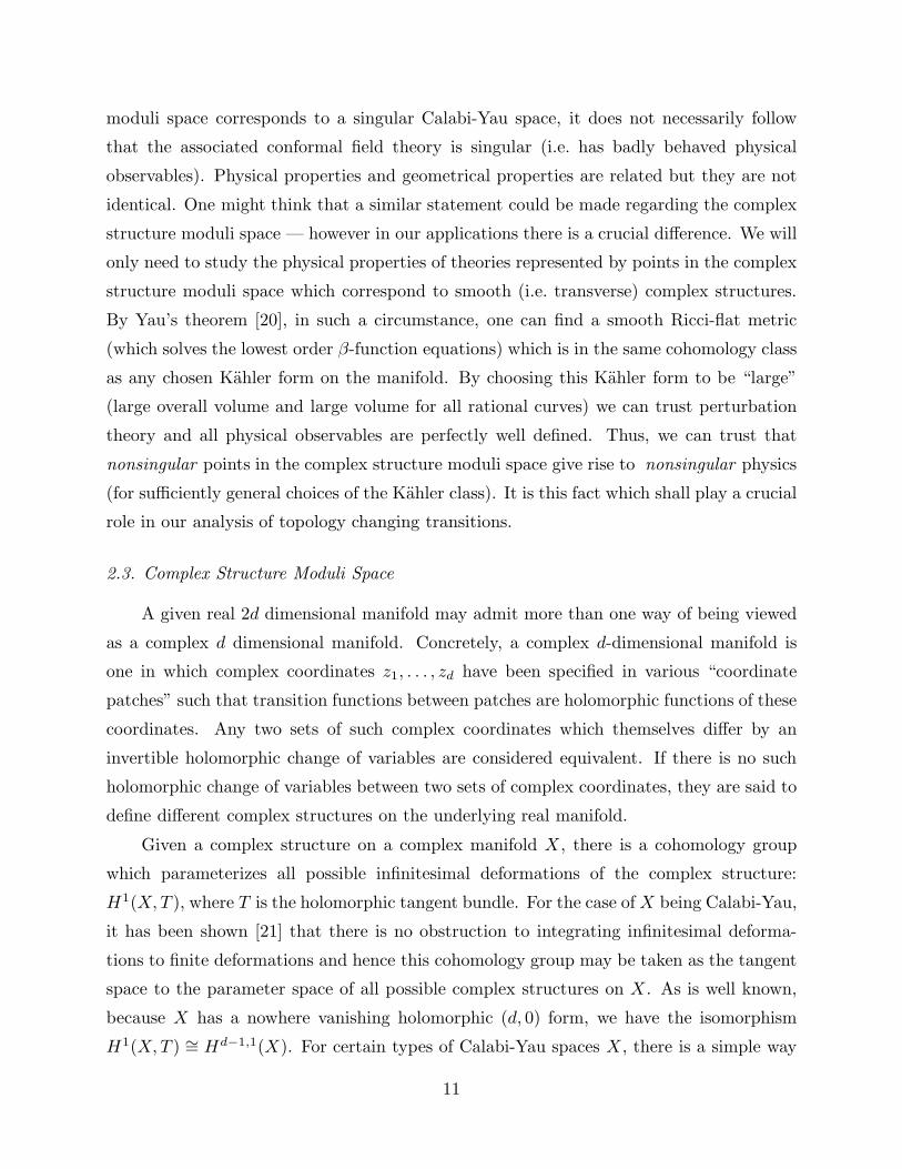
structures, this singularity condition is met on the “discriminant locus” of X , which is a

complex codimension one variety. Being complex codimension one, note (figure 1) that

we can choose a path between any two nonsingular complex structures which avoids the

discriminant locus. This will be a useful fact later on.

4 More precisely, not all choices lead to an X which is “no more singular than it has to be”.

There will be certain singularities of X which arise from singularities of the weighted projective

space itself; we wish to exclude any additional singularities.

12

Discriminant Locus

Figure 1. The moduli space of complex structures.

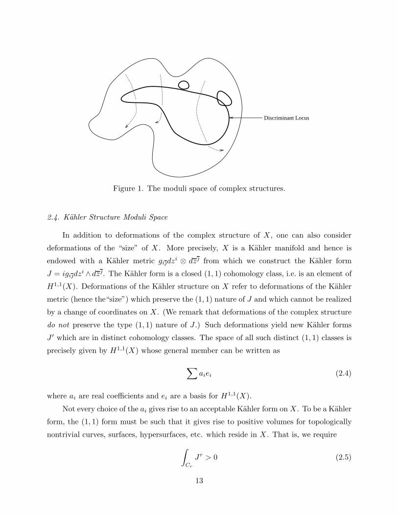
2.4. Kahler Structure Moduli Space

In addition to deformations of the complex structure of X , one can also consider

deformations of the “size” of X . More precisely, X is a Kahler manifold and hence is

endowed with a Kahler metric gidzi ⊗ dz from which we construct the Kahler form

J = igidzi ∧ dz. The Kahler form is a closed (1, 1) cohomology class, i.e. is an element of

H1,1(X). Deformations of the Kahler structure on X refer to deformations of the Kahler

metric (hence the“size”) which preserve the (1, 1) nature of J and which cannot be realized

by a change of coordinates on X . (We remark that deformations of the complex structure

do not preserve the type (1, 1) nature of J .) Such deformations yield new Kahler forms

J ′ which are in distinct cohomology classes. The space of all such distinct (1, 1) classes is

precisely given by H1,1(X) whose general member can be written as

∑aiei (2.4)

where ai are real coefficients and ei are a basis for H1,1(X).

Not every choice of the ai gives rise to an acceptable Kahler form on X . To be a Kahler

form, the (1, 1) form must be such that it gives rise to positive volumes for topologically

nontrivial curves, surfaces, hypersurfaces, etc. which reside in X . That is, we require

∫

Cr

Jr > 0 (2.5)

13

where Cr is a homologically nontrivial effective algebraic r-cycle and Jr denotes J ∧ J ∧

. . . ∧ J (with r factors of J). The Kahler moduli space of X is thus given by a cone (the

“Kahler cone”) which consists of those (1, 1) forms which satisfy (2.5). This is a real space

whose dimension is h1,1.

To gain a better understanding of the Kahler moduli space, it proves worthwhile to

study (2.5) in the special case of r = 1 — that is, the case in which Cr is a curve. We

consider a curve C with the property that the limiting condition∫

CJ = 0 can be achieved

while simultaneously maintaining all of the remaining conditions in (2.5) for all5 other

curves, and for all higher dimensional subspaces. These inequalities (and equality) define

a “boundary wall” in the moduli space. We can approach this wall by changing the Kahler

metric so as to shrink the volume of the curve C to a value which is arbitrarily small.

The limiting wall is defined as the place in moduli space where the volume of C has been

shrunk to zero — one says that C has been “blown down” to a point. What happens if

one goes even further and allows the ai in (2.4) to take on values which pass through to

the other side of the wall? Formally, the volume of the curve C would appear to become

negative. This uncomfortable conclusion, though, can have a very natural resolution. The

curve C can actually have positive volume on the other side of the wall, however it must

be viewed as residing on a topologically different space6. This procedure of blowing a curve

C down to a point and then restoring it to positive volume (“blowing up”) in a manner

which changes the topology of the underlying space is known as “flopping”. We can think

of this flopping operation of algebraic geometry as providing a means of traversing a wall7

of the Kahler cone by passing through a singular space and then on to a different smooth

5 In practice, we may need to allow the condition∫

CiJ = 0 to hold for a finite number of

holomorphic curves Ci, all of which lie in the same cohomology class as C. It is crucial for this

discussion that there be only finitely many such curves.6 This interpretation of the volumes is implicit in the analysis of [23], which studied the metric

behavior of the conifold transitions. It has also been considered in the mathematics literature

[24]. The topology changing property of these transformations was first pointed out by Tian and

Yau [9]; see [25] for an update.7 It must be stressed that not every wall of the Kahler moduli space has this property—this

only happens for the so-called “flopping walls”. There are other walls, at which certain families

of curves also shrink down to zero, for which the change upon crossing the wall is not of this

geometric type, but rather, a new kind of physical theory is born. In the simplest cases, after

shrinking down the curves we will have orbifold singularities, and previous “blowup modes” go

over into “twist field modes”. We will encounter some of these other walls in section VI.

14

topological model. Typically there may be many algebraic curves on X which define this

kind of wall of the Kahler cone and so can be flopped on in this way. Each of these flopped

models has its own Kahler cone with walls determined in the manner just described. Our

discussion, therefore, leads to the natural suggestion that we enlarge our perspective on

the Kahler moduli space so as to include all of these Kahler cones glued together along

their common walls. We will call this the “partially enlarged moduli space” for reasons

which shall become clear in section VI.

We emphasize that in passing through a wall (i.e. in flopping a curve) the Hodge

numbers of X remain invariant. Thus, the topology change involved here is different from

that, for example, encountered in the conifold transitions of [11]. However, more refined

topological invariants do change. For instance, the intersection forms on flopped models

generally do differ from one another. Again, we shall see this explicitly in an example in

section V.

So much for the mathematical description of the space of Kahler forms on a Calabi-

Yau manifold and on its flopped versions. Conformal field theory instructs us to modify

our picture of the Kahler moduli space in two important ways.

First, as discussed, there are quantum corrections to this classical analysis which in

general prove difficult to calculate exactly. We will get on a handle on such corrections by

appealing to mirror symmetry.

Second, we have noted that the real dimension of the Kahler moduli space is equal to

h1,1. Conformal field theory instructs us to double this dimension to complex dimension

h1,1 by combining our real Kahler form J with the antisymmetric tensor field B to form

a complexified Kahler form K = B + iJ . The motivation for doing this comes from su-

persymmetry transformations which show that it is precisely this combination that forms

the scalar component of a spacetime superfield. Our discussion concerning the conditions

on J carries through unaltered — being now applied to the imaginary part of K. There

are no constraints on the (1, 1) class B — however, the conformal field theory is invari-

ant under shifts in B by integral (1, 1) classes, i.e. elements of H2(X,Z). Incorporating

this symmetry naturally leads us to exponentiate the naıve coordinates on Kahler moduli

space and consider the true coordinates to be wk = e2πi(Bk+iJk) where Bk and Jk are the

components of the two-forms B and J relative to an integral basis of H2(X,Z). In terms

of these exponentiated complex coordinates, the adjacent Kahler cones of the partially en-

larged moduli space (figure 2) now become bounded domains attached along their common

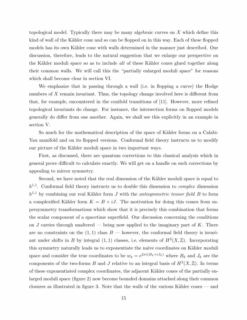
closures as illustrated in figure 3. Note that the walls of the various Kahler cones — and

15

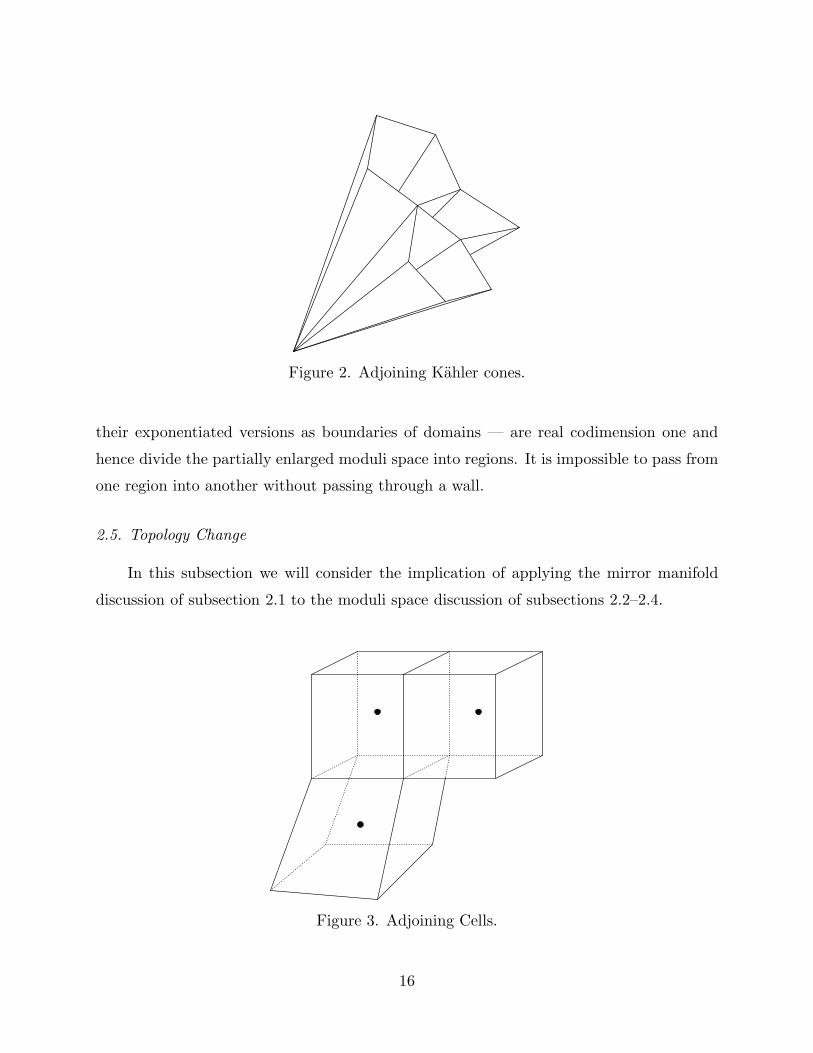
Figure 2. Adjoining Kahler cones.

their exponentiated versions as boundaries of domains — are real codimension one and

hence divide the partially enlarged moduli space into regions. It is impossible to pass from

one region into another without passing through a wall.

2.5. Topology Change

In this subsection we will consider the implication of applying the mirror manifold

discussion of subsection 2.1 to the moduli space discussion of subsections 2.2–2.4.

Figure 3. Adjoining Cells.

16

As we have discussed, if X and Y are a pair of mirror Calabi-Yau spaces, their

corresponding conformally invariant nonlinear σ-models are isomorphic. We mentioned

earlier that the explicit isomorphism involves a change in sign of the left-moving U(1)

charge of the N = 2 superconformal algebra. From our discussion of subsection 2.2 we

therefore see that this isomorphism maps complex structure moduli of X to Kahler moduli

of Y and vice versa. Even as a local result this is a remarkable statement — mathematically

X and Y are a priori unrelated Calabi-Yau spaces. Mirror symmetry establishes, though,

a physical link — their common conformal field theory. Furthermore, the roles played

by the complex and Kahler structure moduli of X and Y are reversed in the associated

physical model. As a global result which claims an isomorphism between the full quantum

mechanical Kahler moduli space of X and the complex structure moduli space of Y and

vice versa, the statement harbors great potential but also raises a confusing issue. If we

compare figures 1 and 3 we are led to ask: how is it possible for these two spaces to be

isomorphic when manifestly they have different structures? Specifically, figure 3 is divided

up into cells with the cell walls corresponding to singular Calabi-Yau spaces lying at the

transition between distinct topological types. In figure 1, however, the space contains no

such cell division. Rather, there are real codimension two subspaces parametrizing singular

complex structures. In figure 3, the passage from one cell to another necessarily passes

through a wall, while in figure 1 — by judicious choice of path — we can pass between any

two nonsingular complex structures without encountering a singularity. So, the puzzle we

are faced with is how are these seemingly distinct spaces isomorphic?

There is another compelling way of stating this question. As mentioned, in the known

construction of mirror pairs [5], typically both of the geometric spaces X0 and Y0 have

quotient singularities. We know that string propagation on such singular spaces, say X0,

is well defined [1] because the string effectively resolves the singularities. However, in

some situations there is more than one way of repairing the singularities giving rise to

topologically distinct smooth spaces. Resolving singularities therefore involves a choice

of desingularization8. These manifolds differ by flops [10]. The moduli space of Calabi-

Yau manifolds takes the form of figure 3. (This partially enlarged moduli space does

not include the point corresponding to the Landau-Ginzburg theory but this will not be

8 Stating this more carefully, bearing in mind that we have actually had to vary parameters

from an initial Landau-Ginzburg theory to arrive at X0, we are asserting that by a further variation

of parameters X0 can deformed into more than one Calabi-Yau manifold.

17

important until later in this paper.) On the mirror to X , namely Y , one would expect

to find some corresponding choices in the complex structure moduli space. In figure 1,

however, there are no divisions into regions, no topological choices to be made. Thus,

what is the physical significance of the topologically distinct regions of figure 3?

Two possible answers to these questions immediately present themselves, however

neither is at first sight convincing. First, it might be that only one region in figure 3

has a physical interpretation and this region would correspond under mirror symmetry

to the whole complex structure moduli space of Y . This explanation implies that the

operation of flopping rational curves (passing through a wall in figure 3) has no conformal

field theory (and hence no physical) realization. Furthermore, it helps to resolve the

asymmetry between figures 1 and 3 as neither, effectively, would be divided into regions.

This explanation would imply that of all the possible resolutions of singularities of X0

— which are on completely equal footing from the mathematical perspective — the string

somehow picks out one. Although unnatural, a priori the string might make some physical

distinction between these possibilities.

As a second possible resolution of the puzzle, it might be that all of the regions in figure

3 are realized by physical models but, as mentioned, this is not immediately convincing

because the walls dividing the Kahler moduli space in figure 3 into topologically distinct

regions have no counterpart in the complex structure moduli space of the mirror. However,

it is important to realize that our discussion of figures 1 and 3 has been based on classical

mathematical analysis. As discussed earlier, although we can trust that nonsingular points

in the complex structure moduli space correspond to nonsingular physical models it is

generally incorrect to conclude that singular points in the Kahler moduli space correspond

to singular physical models. It is therefore possible that the quantum version of figures 2

and 3 are isomorphic with generic points on the walls of the classical version of figure 3

corresponding to nonsingular physical models. In particular, this would imply that one

can pass from one topological type to another in figure 3 — necessarily passing through

a singular Calabi-Yau space — without encountering a physical singularity. Notice that

the mirror description of such a process does not involve topology change. Rather, it

simply involves a continuous and smooth change in the complex structure of the mirror

space (analogous to continuously changing the τ parameter for a torus). Thus, this second

resolution would establish that certain topology changing processes (corresponding to flops

of rational curves) are no more exotic than — and by mirror symmetry can equally well

be described as — smooth changes in the shape of spacetime.

18

In [8], we gave compelling evidence that the latter possibility is in fact correct and

we refer to this resolution as giving rise to multiple mirror manifolds. It is as if a single

topological type (focusing on the complex structure moduli space of Y ) has not one but

many topological images in its mirror reflection (in the partially enlarged Kahler moduli

space of X). Mirror manifolds thus yield a rich catoptric-like moduli space geometry. To

avoid confusion, though, note that a fixed conformal field theory in our family still has

precisely two geometrical interpretations.

We established this picture of topology change in [8] by verifying an extremely sensitive

prediction of this scenario which we now review. In section VI we will also describe a means

of identifying the fully enlarged Kahler moduli space of X with the complex structure

moduli space of Y by means of concepts from toric geometry.

Let X and Y be a mirror pair of Calabi-Yau manifolds. Because they are a mirror

pair, a striking and extremely useful equality between the Yukawa couplings amongst the

(1, 1) forms on M and the (2, 1) forms on Y (and vice versa) is satisfied. This equality

demands that [5]:

∫

Y

ωabcb(i)a ∧ b(j)b ∧ b(k)

c ∧ ω = (2.6)

∫

X

b(i) ∧ b(j) ∧ b(k) +∑

m,{u}

e

∫P1

u∗mK

(∫

P1

u∗b(i)∫

P1

u∗b(j)∫

P1

u∗b(k)

).

where on the left hand side (as derived in [26]) the b(i)a are (2, 1) forms (expressed as ele-

ments of H1(Y, T ) with their subscripts being tangent space indices), ω is the holomorphic

three form and on the right hand side (as derived in [27,28,29,30]) the b(i) are (1, 1) forms

on X , {u} is the set of holomorphic maps to rational curves on X , u : P1 → Γ (with Γ such

a holomorphic curve), πm is an m-fold cover P1 → P1 and um = u ◦ πm. One should note

that the left-hand side of (2.6) is independent of Kahler form information of Y and the

right-hand side is independent of the complex structure of X . In particular (2.6) can still

be valid when Y has rational singularities with Kahler resolutions since such a singular Y

may be thought of as a smooth Y ′ with a deformation of Kahler form.

Notice the interesting fact that forX at “large radius” (i.e., when | exp(∫P1 u

∗mK)| ≪ 1,

for all u) the right hand side of (2.6) reduces to the topological intersection form on X and

hence mirror symmetry (in this particular limit) equates a topological invariant of X to a

19

quasitopological invariant (i.e., one depending on the complex structure) of Y [5].9 In a

simple case a suitable limit was found in [33] such that the intersection form of a manifold

could indeed be calculated from its mirror partner in this way. If the multiple mirror

manifold picture is correct, and all regions of figure 3 are physically realized, the following

must hold: Each of the distinct intersection forms, which represents the large radius limit

of the (1, 1) Yukawa couplings on each of the topologically distinct resolutions of X0, must

be equal to the (2, 1) Yukawa couplings on Y for suitable corresponding “large complex

structure” limits. That is, if there are N distinct resolutions of X0, one should be able

to perform a calculation along the lines of [33] such that N different sets of intersection

numbers are obtained by taking N different limits. We schematically illustrate these limits

by means of the marked points in the interiors of the regions in figure 3. We emphasize

that checking (2.6) in the large radius limit makes the calculation much more tractable

but it does not in any way compromise our results. This is an extremely sensitive test of

the global picture of topology change and of moduli space that we are presenting. Now,

actually invoking this equality requires understanding the precise complex structure limits

that correspond, under mirror symmetry, to the particular large Kahler structure limits

being taken. In the simple case studied in [33] it was possible to use discrete symmetries

to make a well-educated guess at the desired large complex structure. That example did

not admit any flops however. It appears almost inevitable that any example which has

the required complexity to admit flops will be too difficult to approach along the lines

of [33]. What we are in need of then is a more sophisticated way of knowing which large

complex limits are to be identified with which intersection numbers of the mirror manifold.

It turns out that the mathematical machinery of toric geometry provides the appropriate

tools for discussing these moduli spaces and hence for finding these limit points in the

complex structure moduli space. Thus, in the next section we shall give a brief primer

on the subject of toric geometry, in section IV we shall apply these concepts to mirror

symmetry and in section V we shall examine an explicit example.

9 In [29] equation (2.6) was combined with an explicit determination of the mirror map (the

map between the Kahler moduli space of X and the complex structure moduli space of X/G for

X being the Fermat quintic in P4) to determine the number of rational curves of arbitrary degree

on (deformations of) X. This calculation has subsequently been described mathematically [31]

and extended to a number of other examples [32].

20

3. A Primer on Toric Geometry

In this section we give an elementary discussion of toric geometry emphasizing those

points most relevant to the present work. For more details and proofs the reader should

consult [34,35].

3.1. Intuitive Ideas

Toric geometry describes the structure of a certain class of geometrical spaces in

terms of simple combinatorial data. When a space admits a description in terms of toric

geometry, many basic and essential characteristics of the space — such as its divisor classes,

its intersection form and other aspects of its cohomology — are neatly coded and easily

deciphered from analysis of corresponding lattices. We will describe this more formally in

the following subsections. Here we outline the basic ideas.

A toric variety V over C (one can work over other fields but that shall not concern us

here) is a complex geometrical space which contains the algebraic torus T = C∗×. . .×C

∗ ∼=

(C∗)n as a dense open subset. Furthermore, there is an action of T on V ; that is, a map

T × V → V which extends the natural action of T on itself. The points in V − T can

be regarded as limit points for the action of T on itself; these serve to give a partial

compactification of T . Thus, V can be thought of as a (C∗)n together with additional

limit points which serve to partially (or completely) compactify the space10. Different

toric varieties V , therefore, are distinguished by their different compactifying sets. The

latter, in turn, are distinguished by restricting the limits of the allowed action of T —

and these restrictions can be encoded in a convenient combinatorial structure as we now

describe.

In the framework of an action T×V → V we can focus our attention on one-parameter

subgroups of the full T action11. Basically, we follow all possible holomorphic curves in

T as they act on V , and ask whether or not the action has a limit point in V . As the

algebraic torus T is a commutative algebraic group, all of its one-parameter subgroups are

10 As we shall see in the next subsection, this discussion is a bit naıve — these spaces need not

be smooth, for instance. Hence it is not enough just to say what points are added — we must

also specify the local structure near each new point.11 We use subgroups depending on one complex parameter.

21

labeled by points in a lattice N ∼= Zn in the following way. Given (n1, . . . , nn) ∈ Z

n and

λ ∈ C∗ we consider the one-parameter group C

∗ acting on V by

λ× (z1, . . . , zn) → (λn1z1, . . . , λnnzn) (3.1)

where (z1, . . . , zn) are local holomorphic coordinates on V (which may be thought of as

residing in the open dense (C∗)n subset of V ). Now, to describe all of V (that is, in

addition to T ) we consider the action of (3.1) in the limit that λ approaches zero (and thus

moves from C∗ into C). It is these limit points which supply the partial compactifications

of T thereby yielding the toric variety V . The limit points obtained from the action

(3.1) depend upon the explicit vector of exponents (n1, . . . , nn) ∈ Zn, but many different

exponent-vectors can give rise to the same limit point. We obtain different toric varieties

by imposing different restrictions on the allowed choices of (n1, . . . , nn), and by grouping

them together (according to common limit points) in different ways.

We can describe these restrictions and groupings in terms of a “fan” ∆ in N which

is a collection of strongly convex rational polyhedral cones σi in the real vector space

NR = N ⊗Z R. (In simpler language, each σi is a convex cone with apex at the origin

spanned by a finite number of vectors which live in the lattice N and such that any angle

subtended by these vectors at the apex is < 180◦.) The fan ∆ is a collection of such

cones which satisfy the requirement that the face of any cone in ∆ is also in ∆. Now,

in constructing V , we associate a coordinate patch of V to each large cone12 σi in ∆,

where large refers to a cone spanning an n-dimensional subspace of N . This patch consists

of (C∗)n together with all the limit points of the action (3.1) for (n1, . . . , nn) restricted

to lie in σi ∩ N . There is a single point which serves as the common limit point for all

one-parameter group actions with vector of exponents (n1, . . . , nn) lying in the interior of

σi; for exponent-vectors on the boundary of σi, additional families of limit points must be

adjoined.

We glue these patches together in a manner dictated by the precise way in which the

cones σ adjoin each other in the collection ∆. Basically, the patches are glued together in

a manner such that the one-parameter group actions in the two patches agree along the

12 There are also coordinate patches for the smaller cones, but we ignore these for the present.

22

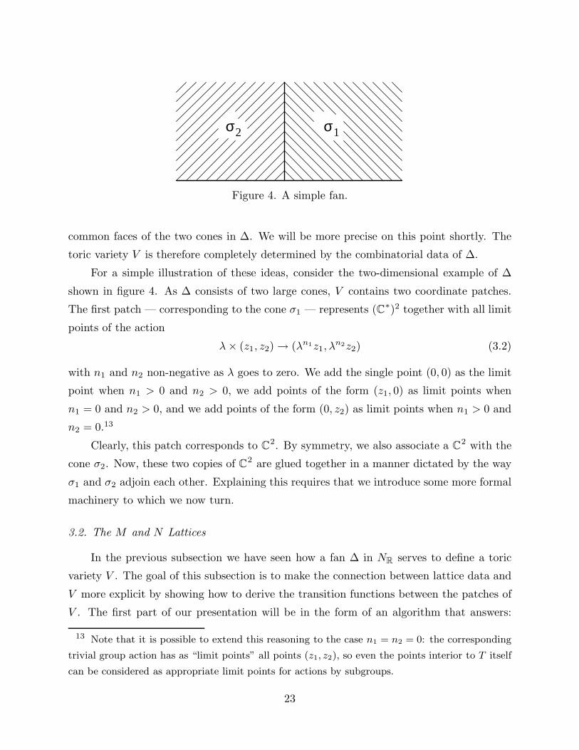
σσ 12

Figure 4. A simple fan.

common faces of the two cones in ∆. We will be more precise on this point shortly. The

toric variety V is therefore completely determined by the combinatorial data of ∆.

For a simple illustration of these ideas, consider the two-dimensional example of ∆

shown in figure 4. As ∆ consists of two large cones, V contains two coordinate patches.

The first patch — corresponding to the cone σ1 — represents (C∗)2 together with all limit

points of the action

λ× (z1, z2) → (λn1z1, λn2z2) (3.2)

with n1 and n2 non-negative as λ goes to zero. We add the single point (0, 0) as the limit

point when n1 > 0 and n2 > 0, we add points of the form (z1, 0) as limit points when

n1 = 0 and n2 > 0, and we add points of the form (0, z2) as limit points when n1 > 0 and

n2 = 0.13

Clearly, this patch corresponds to C2. By symmetry, we also associate a C

2 with the

cone σ2. Now, these two copies of C2 are glued together in a manner dictated by the way

σ1 and σ2 adjoin each other. Explaining this requires that we introduce some more formal

machinery to which we now turn.

3.2. The M and N Lattices

In the previous subsection we have seen how a fan ∆ in NR serves to define a toric

variety V . The goal of this subsection is to make the connection between lattice data and

V more explicit by showing how to derive the transition functions between the patches of

V . The first part of our presentation will be in the form of an algorithm that answers:

13 Note that it is possible to extend this reasoning to the case n1 = n2 = 0: the corresponding

trivial group action has as “limit points” all points (z1, z2), so even the points interior to T itself

can be considered as appropriate limit points for actions by subgroups.

23

given the fan ∆ how do we explicitly define coordinate patches and transition functions

for the toric variety V ? We will then briefly describe the mathematics underlying the

algorithm.

Towards this end, it proves worthwhile to introduce a second lattice defined as the

dual lattice to N , M = Hom(N,Z). We denote the dual pairing of M and N by 〈, 〉.

Corresponding to the fan ∆ in NR we define a collection of dual cones σi in MR via

σi = {m ∈MR : 〈m,n〉 ≥ 0 for all n ∈ σi}. (3.3)

Now, for each dual cone σi we choose a finite set of elements {mi,j ∈M} (with j = 1, . . . , ri)

such that

σi ∩M = Z≥0mi,1 + . . .+ Z≥0mi,ri. (3.4)

We then find a finite set of relations

ri∑

j=1

ps,jmi,j = 0 (3.5)

with s = 1, . . . , R such that any relation

ri∑

j=1

pjmi,j = 0 (3.6)

can be written as a linear combination of the given set, with integer coefficients. (That is,

pj =∑R

s=1 µsps,j for some integers µs.) We associate a coordinate patch Uσito the cone

σi ∈ ∆ by

Uσi= {(ui,1, . . . , ui,ri

) ∈ Cri | ui,1

ps,1ui,2ps,2 . . . ui,ri

ps,ri = 1 for all s}, (3.7)

the equations representing constraints on the variables ui,1, . . . , ui,ri. We then glue these

coordinate patches Uσiand Uσj

together by finding a complete set of relations of the form

ri∑

l=1

qlmi,l +

rj∑

l=1

q′lmj,l = 0 (3.8)

where the ql and q′l are integers. For each of these relations we impose the coordinate

transition relation

ui,1q1ui,2

q2 . . . ui,ri

qruj,1q′1uj,2

q′2 . . . uj,rj

q′r = 1. (3.9)

24

This algorithm explicitly shows how the lattice data encodes the defining data for the toric

variety V .

Before giving a brief description of the mathematical meaning behind this algorithm,

we pause to illustrate it in two examples. First, let us return to the fan ∆ given in figure

4. It is straightforward to see that the dual cones, in this case, take precisely the same

form as in figure 4. We have m1,1 = (1, 0), m1,2 = (0, 1);m2,1 = (−1, 0), m2,2 = (0, 1). As

the basis vectors within a given patch are linearly independent, each patch consists of a

C2. To glue these two patches together we follow (3.8) and write the set of relations

m1,1 +m2,1 = 0 (3.10)

m1,2 −m2,2 = 0. (3.11)

These yield the transition functions

u1,1 = u−12,1 , u1,2 = u2,2. (3.12)

These transition functions imply that the corresponding toric variety V is the space P1×C.

σ

σ

σ1

2

3

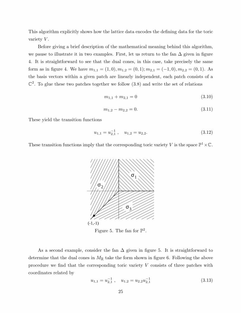
(-1,-1)

Figure 5. The fan for P2.

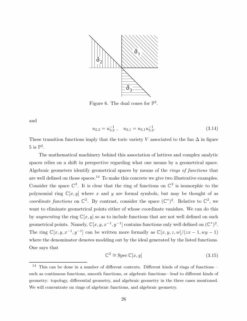
As a second example, consider the fan ∆ given in figure 5. It is straightforward to

determine that the dual cones in MR take the form shown in figure 6. Following the above

procedure we find that the corresponding toric variety V consists of three patches with

coordinates related by

u1,1 = u−12,1 , u1,2 = u2,2u

−12,1 (3.13)

25

σ1

σ

σ

2

3

Figure 6. The dual cones for P2.

and

u2,2 = u−13,2 , u2,1 = u3,1u

−13,2. (3.14)

These transition functions imply that the toric variety V associated to the fan ∆ in figure

5 is P2.

The mathematical machinery behind this association of lattices and complex analytic

spaces relies on a shift in perspective regarding what one means by a geometrical space.

Algebraic geometers identify geometrical spaces by means of the rings of functions that

are well defined on those spaces.14 To make this concrete we give two illustrative examples.

Consider the space C2. It is clear that the ring of functions on C

2 is isomorphic to the

polynomial ring C[x, y] where x and y are formal symbols, but may be thought of as

coordinate functions on C2. By contrast, consider the space (C∗)2. Relative to C

2, we

want to eliminate geometrical points either of whose coordinate vanishes. We can do this

by augmenting the ring C[x, y] so as to include functions that are not well defined on such

geometrical points. Namely, C[x, y, x−1, y−1] contains functions only well defined on (C∗)2.

The ring C[x, y, x−1, y−1] can be written more formally as C[x, y, z, w]/(zx − 1, wy − 1)

where the denominator denotes modding out by the ideal generated by the listed functions.

One says that

C2 ∼= Spec C[x, y] (3.15)

14 This can be done in a number of different contexts. Different kinds of rings of functions—

such as continuous functions, smooth functions, or algebraic functions—lead to different kinds of

geometry: topology, differential geometry, and algebraic geometry in the three cases mentioned.

We will concentrate on rings of algebraic functions, and algebraic geometry.

26

and

(C∗)2 ∼= SpecC[x, y, z, w]

(zx− 1, wy − 1)(3.16)

where the term “Spec” may intuitively be thought of as “the minimal space of points where

the following function ring is well defined”.

With this terminology, the coordinate patch Uσicorresponding to the cone σi in a fan

∆ is given by

Uσi∼= Spec C[σi ∩M ] (3.17)

where by σi∩M we refer to the monomials in local coordinates that are naturally assigned

to lattice points in M by virtue of its being the dual space to N . Explicitly, a lattice point

(m1, . . . , mn) in M corresponds to the monomial zm1

1 zm2

2 . . . zmnn . The latter are sometimes

referred to as group characters of the algebraic group action given by T .

Within a given patch, Spec C[σi∩M ] is a polynomial ring generated by the monomials

associated to the lattice points in σi. By the map given in the previous paragraph between

lattice points and monomials, we see that linear relations between lattice points translate

into multiplicative relations between monomials. These relations are precisely those given

in (3.5).

Between patches, if σi and σj share a face, say τ , then C[σi ∩M ] and C[σj ∩M ] are

both subalgebras of C[τ ∩M ]. This provides a means of identifying elements of C[σi ∩M ]

and elements of C[σj ∩ M ] which translates into a map between Spec C[σi ∩ M ] and

Spec C[σj ∩M ]. This map is precisely that given in (3.9).

3.3. Singularities and their Resolution

In general, a toric variety V need not be a smooth space. One advantage of the toric

description is that a simple analysis of the lattice data associated with V allows us to

identify singular points. Furthermore, simple modifications of the lattice data allow us to

construct from V a toric variety V in which all of the singular points are repaired. We

now briefly describe these ideas.

The essential result we need is as follows:

Let V be a toric variety associated to a fan ∆ in N . V is smooth if for each cone σ

in the fan we can find a Z basis {n1, . . . , nn} of N and an integer r ≤ n such that

σ = R≥0 n1 + . . .+ R≥0 nr.

27

For a proof of this statement the reader should consult, for example, [34] or [35]. The

basic idea behind the result is as follows. If V satisfies the criterion in the proposition,

then the dual cone σ to σ can be expressed as

σ =

r∑

i=1

R≥0mi +

n∑

i=r+1

Rmi (3.18)

where {m1, . . . , mn} is the dual basis to {n1, . . . , nn}. We can therefore write

σ ∩M =

r∑

i=1

Z≥0mi +

n∑

i=r+1

Z≥0mi +

n∑

i=r+1

Z≥0 (−mi). (3.19)

From our prescription of subsection 3.2, this patch is therefore isomorphic to

SpecC[x1, . . . , xn, yr+1, . . . , yn]∏n

i=r+1(xiyi − 1). (3.20)

In plain language, this is simply Cr × (C∗)n−r, which is certainly nonsingular. The key

to this patch being smooth is that σ is r-dimensional and it is spanned by r linearly

independent lattice vectors in N . This implies, via the above reasoning, that there are no

“extra” constraints on the monomials associated with basis vectors in the patch (see (3.7))

hence leaving a smooth space.

Of particular interest in this paper will be toric varieties V whose fan ∆ is simplicial.

This means that each cone σ in the fan can be written in the form σ = R≥0 n1 + . . . +

R≥0 nr for some linearly independent vectors n1, . . . , nr ∈ N . (Such a cone is itself called

simplicial.) When r = n, we define a “volume” for simplicial cones as follows: choose

each nj to be the first nonzero lattice point on the ray R≥0 nj and define vol(σ) to be the

volume of the polyhedron with vertices O, n1, . . . , nn. (We normalize our volumes so that

the unit simplex in Rn (with respect to the lattice N) has volume 1. Then the volume of σ

coincides with the index [N : Nσ], where Nσ is the lattice generated by n1, . . . , nn.) Note

that the coordinate chart Uσ associated to a simplicial cone σ of dimension n is smooth at

the origin precisely when vol(σ) = 1.

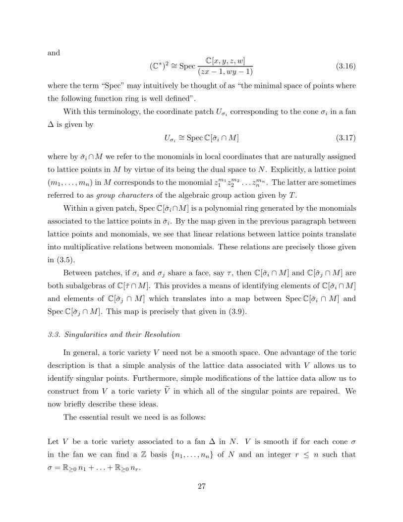
To illustrate this idea, we consider a fan ∆, figure 7, which gives rise to a singular

variety. This fan has one big (simplicial) cone of volume 2 generated by v1 = (0, 1) = n1

and v2 = (2, 1) = n1 +2n2. The dual cone σ is generated by w1 = (2,−1) = 2m1 −m2 and

w2 = (0, 1) = m2. In these expressions, ni and mj are the standard basis vectors. It is clear

that this toric variety is not smooth since it does not meet the conditions of the proposition.

28

(0,1)(2,1)

Figure 7. The fan for C/Z2.

More explicitly, following (3.7) we see that σ∩M = Z≥0 (2m1−m2)+Z≥0 (m2)+Z≥0 (m1)

and hence V = Spec(C[x, y, z]/(z2 − xy = 0)). In plain language, V is the vanishing locus

of z2 − xy in C3. This is singular at the origin, as is easily seen by the transversality test.

Alternatively, a simple change of variables; z = u1u2, x = u21, y = u2

2, reveals that V is in

fact C2/Z2 (with Z2 generated by the action (u1, u2) → (−u1,−u2)) which is singular at

the origin as this is a fixed point. Notice that the key point leading to this singularity is

the fact that we require three lattice vectors to span the two dimensional sublattice σ∩M .

The proposition and this discussion suggest a procedure to follow to modify any such

V so as to repair singularities which it might have. Namely, we construct a new fan ∆

from the original fan ∆ by subdividing: first subdividing all cones into simplicial ones, and

then subdividing the cones σi of volume > 1 until the stipulations of the nonsingularity

proposition are met. The new fan ∆ will then be the toric data for a nonsingular resolution

of the original toric variety V . This procedure is called blowing-up. We illustrate it with

our previous example of V = C2/Z2. Consider constructing ∆ by subdividing the cone

in ∆ into two pieces by a ray passing through the point (1, 1). It is then straightforward

to see that each cone in ∆ meets the smoothness criterion. By following the procedure of

subsection 3.2 one can derive the transition functions on V and find that it is the total

space of the line bundle O(−2) over P1 (which is smooth). This is the well known blow-up

of the quotient singularity C2/Z2.

If the volume of a cone as defined above behaved the way one might hope, i.e., when-

ever dividing a cone of volume v into other cones, one produced new cones whose volumes

summed to v, then subdivision would clearly be a finite process. Unfortunately this is not

29

the case15 and in general one can continue dividing any cone for as long as one has the

patience. This corresponds to the fact that one can blow-up any point on a manifold to

obtain another manifold. In our case, however, we will utilize the fact that string theory

demands that the canonical bundle of a target space is trivial. The Calabi-Yau manifold

will not be the toric variety itself as we will see in subsection 3.5 but we do require that any

resolution of singularities adds nothing new to the canonical class of V . This will restrict

the allowed blowups rather severely.

In order to have a resolution which adds nothing new to the canonical class, the singu-

larities must be what are called canonical Gorenstein singularities [36]. A characterization

of which toric singularities have this property was given by Danilov and Reid. To state

it, consider a cone σ from our fan ∆, and examine the one-dimensional edges of σ. As we

move away from O along any of these edges we eventually reach a point in N . In this way

we associate a collection of points S ⊂ N with σ. (These points will lie in the bound-

ary of a polyhedron P ◦ which we will discuss in more detail in subsection 3.5.) The fact

we require is that the singularities of the affine toric variety Uσ are canonical Gorenstein

singularities if all the points in S lie in an affine hyperplane H in NR of the form

H = {x ∈ NR | 〈m, x〉 = 1} (3.21)

for some m ∈ M , and if there are no lattice points x ∈ σ ∩N with 0 < 〈m, x〉 < 1. ([36],

p.294). Furthermore, in order to avoid adding anything new to the canonical class, we

must choose all one-dimensional cones used in subdividing σ from among rays of the form

R≥0 x where x ∈ σ ∩N lies on the hyperplane H (i.e., 〈m, x〉 = 1).

If we have a big simplicial cone, then the n points in NR associated to the one-

dimensional subcones of this cone always define an affine hyperplane in NR. If we assume

the singularity is canonical and Gorenstein, then this hyperplane is one integral unit away

from the origin and volumes can be conveniently calculated on it. In particular, if the

volume of the big cone is greater than 1 then this hyperplane will intersect more points

in σ ∩ N . These additional points define the one-dimensional cones that can be used for

further subdivisions of the cone that do not affect the canonical class. Since volumes are

calculated in the hyperplane H, the volume property behaves well under such resolutions,

15 If the closest lattice point to the origin on the subdividing ray does not lie on a face of the

polyhedron 〈O, n1, . . . , nn〉 then the new polyhedra will be unrelated to the old, and the volumes

will not add.

30

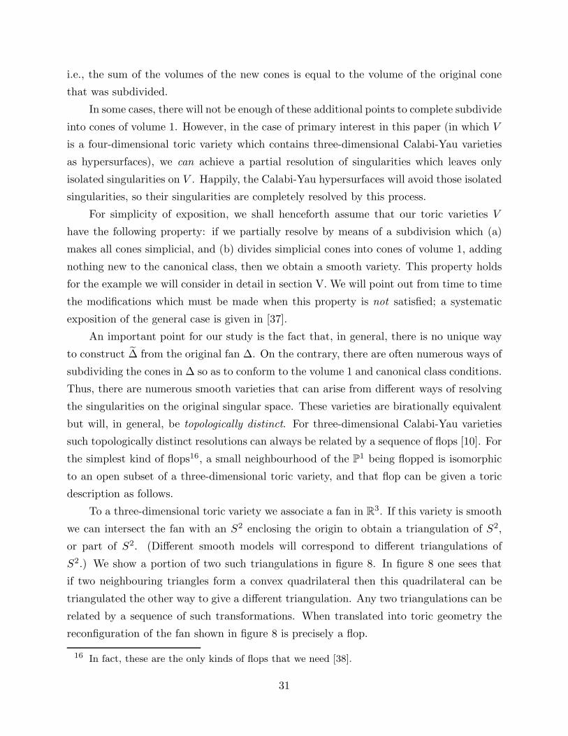
i.e., the sum of the volumes of the new cones is equal to the volume of the original cone

that was subdivided.

In some cases, there will not be enough of these additional points to complete subdivide

into cones of volume 1. However, in the case of primary interest in this paper (in which V

is a four-dimensional toric variety which contains three-dimensional Calabi-Yau varieties

as hypersurfaces), we can achieve a partial resolution of singularities which leaves only

isolated singularities on V . Happily, the Calabi-Yau hypersurfaces will avoid those isolated

singularities, so their singularities are completely resolved by this process.

For simplicity of exposition, we shall henceforth assume that our toric varieties V

have the following property: if we partially resolve by means of a subdivision which (a)

makes all cones simplicial, and (b) divides simplicial cones into cones of volume 1, adding

nothing new to the canonical class, then we obtain a smooth variety. This property holds

for the example we will consider in detail in section V. We will point out from time to time

the modifications which must be made when this property is not satisfied; a systematic

exposition of the general case is given in [37].

An important point for our study is the fact that, in general, there is no unique way

to construct ∆ from the original fan ∆. On the contrary, there are often numerous ways of

subdividing the cones in ∆ so as to conform to the volume 1 and canonical class conditions.

Thus, there are numerous smooth varieties that can arise from different ways of resolving

the singularities on the original singular space. These varieties are birationally equivalent

but will, in general, be topologically distinct. For three-dimensional Calabi-Yau varieties

such topologically distinct resolutions can always be related by a sequence of flops [10]. For

the simplest kind of flops16, a small neighbourhood of the P1 being flopped is isomorphic

to an open subset of a three-dimensional toric variety, and that flop can be given a toric

description as follows.

To a three-dimensional toric variety we associate a fan in R3. If this variety is smooth

we can intersect the fan with an S2 enclosing the origin to obtain a triangulation of S2,

or part of S2. (Different smooth models will correspond to different triangulations of

S2.) We show a portion of two such triangulations in figure 8. In figure 8 one sees that

if two neighbouring triangles form a convex quadrilateral then this quadrilateral can be

triangulated the other way to give a different triangulation. Any two triangulations can be

related by a sequence of such transformations. When translated into toric geometry the

reconfiguration of the fan shown in figure 8 is precisely a flop.

16 In fact, these are the only kinds of flops that we need [38].

31

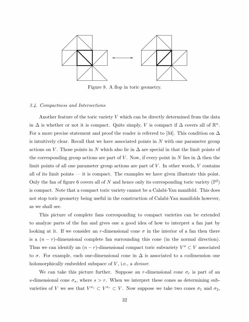
Figure 8. A flop in toric geometry.

3.4. Compactness and Intersections

Another feature of the toric variety V which can be directly determined from the data

in ∆ is whether or not it is compact. Quite simply, V is compact if ∆ covers all of Rn.

For a more precise statement and proof the reader is referred to [34]. This condition on ∆

is intuitively clear. Recall that we have associated points in N with one parameter group

actions on V . Those points in N which also lie in ∆ are special in that the limit points of

the corresponding group actions are part of V . Now, if every point in N lies in ∆ then the

limit points of all one parameter group actions are part of V . In other words, V contains

all of its limit points — it is compact. The examples we have given illustrate this point.

Only the fan of figure 6 covers all of N and hence only its corresponding toric variety (P2)

is compact. Note that a compact toric variety cannot be a Calabi-Yau manifold. This does

not stop toric geometry being useful in the construction of Calabi-Yau manifolds however,

as we shall see.

This picture of complete fans corresponding to compact varieties can be extended

to analyze parts of the fan and gives one a good idea of how to interpret a fan just by

looking at it. If we consider an r-dimensional cone σ in the interior of a fan then there

is a (n − r)-dimensional complete fan surrounding this cone (in the normal direction).

Thus we can identify an (n− r)-dimensional compact toric subvariety V σ ⊂ V associated

to σ. For example, each one-dimensional cone in ∆ is associated to a codimension one

holomorphically embedded subspace of V , i.e., a divisor.

We can take this picture further. Suppose an r-dimensional cone σr is part of an

s-dimensional cone σs, where s > r. When we interpret these cones as determining sub-

varieties of V we see that V σs ⊂ V σr ⊂ V . Now suppose we take two cones σ1 and σ2,

32

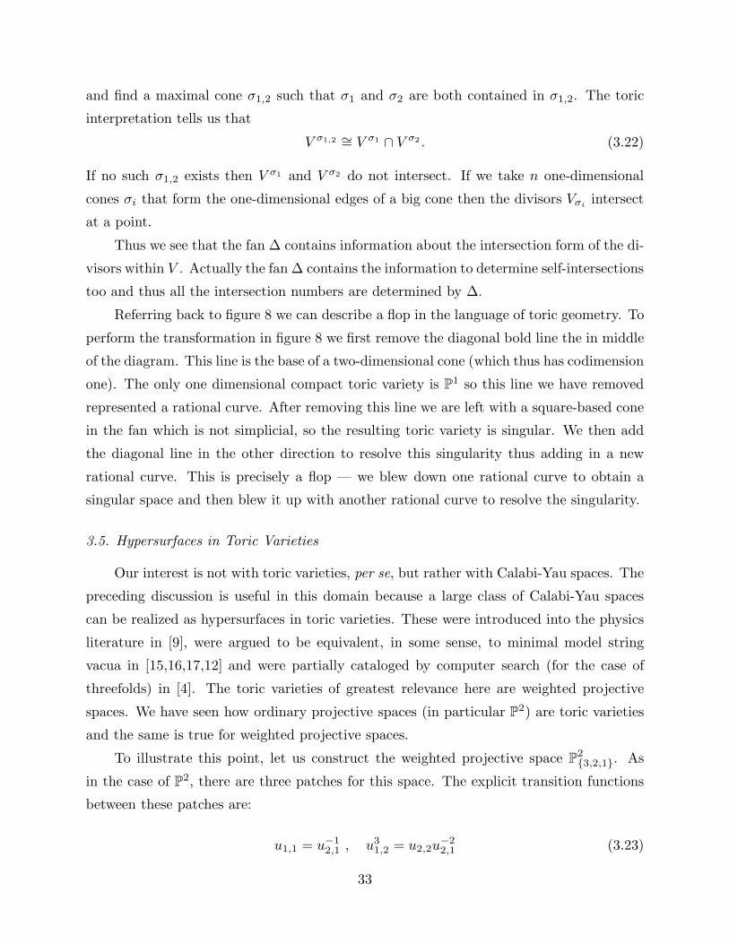
and find a maximal cone σ1,2 such that σ1 and σ2 are both contained in σ1,2. The toric

interpretation tells us that

V σ1,2 ∼= V σ1 ∩ V σ2 . (3.22)

If no such σ1,2 exists then V σ1 and V σ2 do not intersect. If we take n one-dimensional

cones σi that form the one-dimensional edges of a big cone then the divisors Vσiintersect

at a point.

Thus we see that the fan ∆ contains information about the intersection form of the di-

visors within V . Actually the fan ∆ contains the information to determine self-intersections

too and thus all the intersection numbers are determined by ∆.

Referring back to figure 8 we can describe a flop in the language of toric geometry. To

perform the transformation in figure 8 we first remove the diagonal bold line the in middle

of the diagram. This line is the base of a two-dimensional cone (which thus has codimension

one). The only one dimensional compact toric variety is P1 so this line we have removed

represented a rational curve. After removing this line we are left with a square-based cone

in the fan which is not simplicial, so the resulting toric variety is singular. We then add

the diagonal line in the other direction to resolve this singularity thus adding in a new

rational curve. This is precisely a flop — we blew down one rational curve to obtain a

singular space and then blew it up with another rational curve to resolve the singularity.

3.5. Hypersurfaces in Toric Varieties

Our interest is not with toric varieties, per se, but rather with Calabi-Yau spaces. The

preceding discussion is useful in this domain because a large class of Calabi-Yau spaces

can be realized as hypersurfaces in toric varieties. These were introduced into the physics

literature in [9], were argued to be equivalent, in some sense, to minimal model string

vacua in [15,16,17,12] and were partially cataloged by computer search (for the case of

threefolds) in [4]. The toric varieties of greatest relevance here are weighted projective

spaces. We have seen how ordinary projective spaces (in particular P2) are toric varieties

and the same is true for weighted projective spaces.

To illustrate this point, let us construct the weighted projective space P2{3,2,1}. As

in the case of P2, there are three patches for this space. The explicit transition functions

between these patches are:

u1,1 = u−12,1 , u3

1,2 = u2,2u−22,1 (3.23)

33

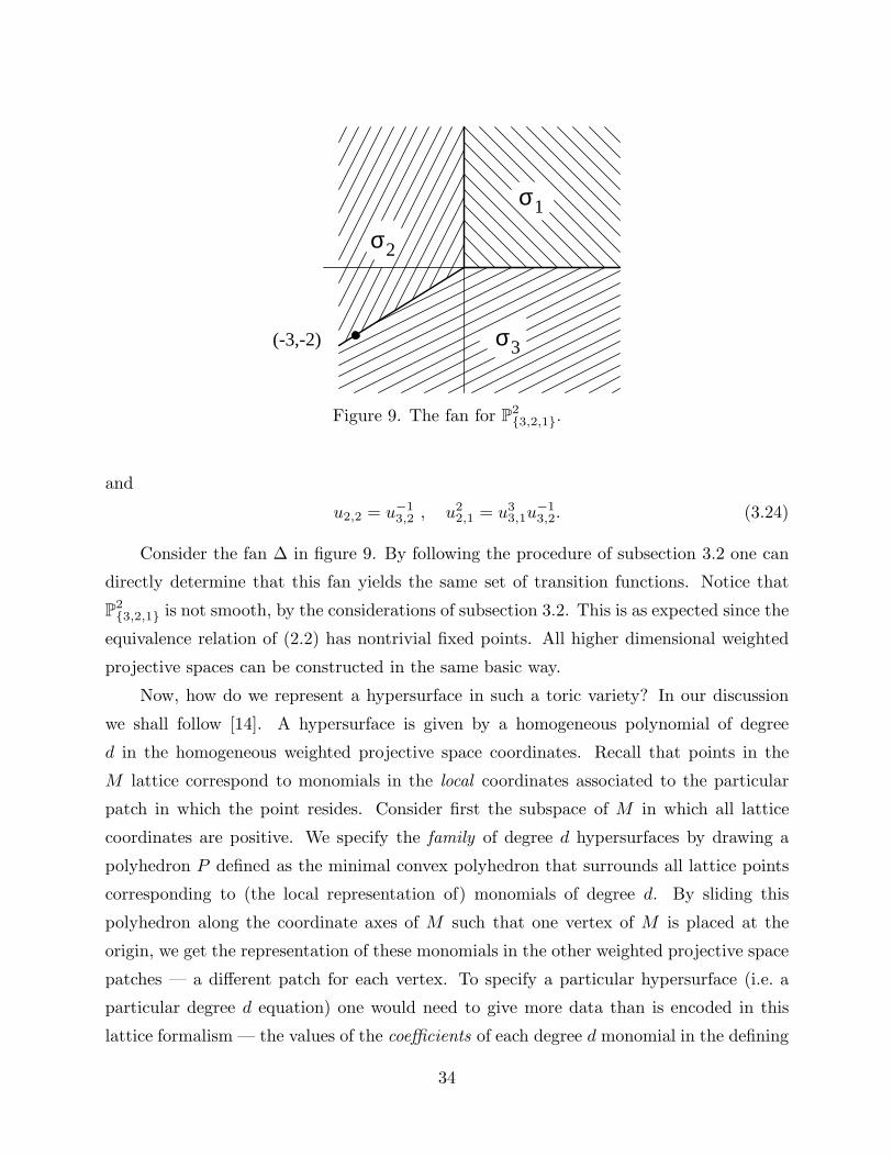
σ

σ

σ1

2

3(-3,-2)

Figure 9. The fan for P2{3,2,1}.

and

u2,2 = u−13,2 , u2

2,1 = u33,1u

−13,2. (3.24)

Consider the fan ∆ in figure 9. By following the procedure of subsection 3.2 one can

directly determine that this fan yields the same set of transition functions. Notice that

P2{3,2,1} is not smooth, by the considerations of subsection 3.2. This is as expected since the

equivalence relation of (2.2) has nontrivial fixed points. All higher dimensional weighted

projective spaces can be constructed in the same basic way.

Now, how do we represent a hypersurface in such a toric variety? In our discussion

we shall follow [14]. A hypersurface is given by a homogeneous polynomial of degree

d in the homogeneous weighted projective space coordinates. Recall that points in the

M lattice correspond to monomials in the local coordinates associated to the particular

patch in which the point resides. Consider first the subspace of M in which all lattice

coordinates are positive. We specify the family of degree d hypersurfaces by drawing a

polyhedron P defined as the minimal convex polyhedron that surrounds all lattice points

corresponding to (the local representation of) monomials of degree d. By sliding this

polyhedron along the coordinate axes of M such that one vertex of M is placed at the

origin, we get the representation of these monomials in the other weighted projective space

patches — a different patch for each vertex. To specify a particular hypersurface (i.e. a

particular degree d equation) one would need to give more data than is encoded in this

lattice formalism — the values of the coefficients of each degree d monomial in the defining

34

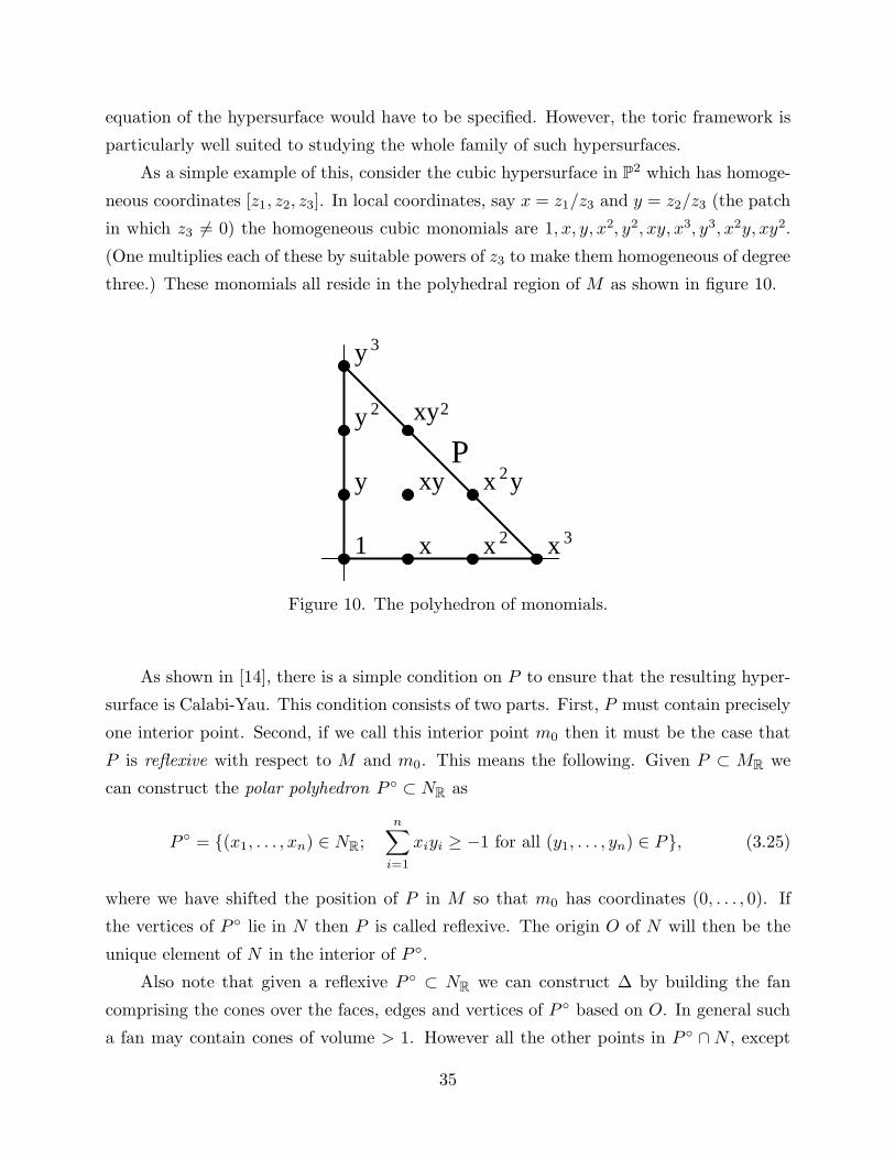
equation of the hypersurface would have to be specified. However, the toric framework is

particularly well suited to studying the whole family of such hypersurfaces.

As a simple example of this, consider the cubic hypersurface in P2 which has homoge-

neous coordinates [z1, z2, z3]. In local coordinates, say x = z1/z3 and y = z2/z3 (the patch

in which z3 6= 0) the homogeneous cubic monomials are 1, x, y, x2, y2, xy, x3, y3, x2y, xy2.

(One multiplies each of these by suitable powers of z3 to make them homogeneous of degree

three.) These monomials all reside in the polyhedral region of M as shown in figure 10.

1 x x x

xy

y

y

xy

2 3

2

2

3

y

xy2

P

Figure 10. The polyhedron of monomials.

As shown in [14], there is a simple condition on P to ensure that the resulting hyper-

surface is Calabi-Yau. This condition consists of two parts. First, P must contain precisely

one interior point. Second, if we call this interior point m0 then it must be the case that

P is reflexive with respect to M and m0. This means the following. Given P ⊂ MR we

can construct the polar polyhedron P ◦ ⊂ NR as

P ◦ = {(x1, . . . , xn) ∈ NR;n∑

i=1

xiyi ≥ −1 for all (y1, . . . , yn) ∈ P}, (3.25)

where we have shifted the position of P in M so that m0 has coordinates (0, . . . , 0). If

the vertices of P ◦ lie in N then P is called reflexive. The origin O of N will then be the

unique element of N in the interior of P ◦.

Also note that given a reflexive P ◦ ⊂ NR we can construct ∆ by building the fan

comprising the cones over the faces, edges and vertices of P ◦ based on O. In general such

a fan may contain cones of volume > 1. However all the other points in P ◦ ∩ N , except

35

O, are on faces and edges of P ◦ and can thus be used to resolve the singularities of V

without affecting the canonical class. The exceptional divisors introduced into V by this

resolution of singularities can intersect the hypersurface to produce exceptional divisors

in the Calabi-Yau manifold. (However, this does not necessarily happen in all cases. If

we consider a point in the interior of a codimension one face of P ◦ then the exceptional

divisor induced in V would not intersect the hypersurface and therefore would give no

contribution to the Calabi-Yau manifold.)

To finish specifying ∆ we must say which sets of the one-dimensional cones are to be

used as the set of edges of a larger cone. Phrased in terms of the relevant lattice points in

P ◦ ∩ N , what we need to specify is a triangulation of P ◦, with vertices in P ◦ ∩ N , each

simplex of which includes O. Replacing each simplex with the corresponding cone whose

vertex lies at O, we produce the fan ∆. Conversely, if we are given ∆ then intersecting the

cones of ∆ with the polyhedron P ◦ produces a triangulation of P ◦.

3.6. Kahler and Complex Structure Moduli

Having seen how Calabi-Yau hypersurfaces in a weighted projective space are de-

scribed in the language of toric geometry we now indicate how the complex structure and

Kahler structure moduli on these spaces are represented.

In general, not all such moduli have a representation in toric geometry. Let’s begin

with complex structure moduli. As discussed in subsection 2.3, such moduli are associ-

ated to elements in Hd−1,1(X), where X is the Calabi-Yau space, and under favorable

circumstances [22] some of these can be represented by monomial perturbations of the

same degree of homogeneity as X . By our discussion of the previous subsection, these are

the lattice points contained within P . Thus, those complex structure deformations with a

monomial representation have a direct realization in the toric description of X .

The other set of moduli are associated with the Kahler structure of X . Note that an

arbitrary element of H1,1(X) can, by Poincare duality, be represented as a (2d− 2)-cycle

in H2d−2(X). As explained in subsection 3.4 and above, divisors in X are given by some

of the one-dimensional cones in ∆ which, in turn, correspond to points in P ◦ ∩N . To be

more precise, by this method, every point in P ◦ ∩N except O and points in codimension

one faces of P ◦ gives a (not necessarily distinct) class in H2d−2(X).

Unfortunately it does not follow that H2d−2(X) is generated by such points in P ◦. In

general an exceptional divisor in V may intersect X in several isolated regions. This leads

to many classes in H2d−2(X) being identified with the same point in P ◦. If we define the

36

Kahler form on X in terms of the cohomology of V we thus restrict to only part of the

moduli space of Kahler forms on X . We will do this in the next subsection, and study

Kahler forms directly on V ; these always induce Kahler forms on X17, and will produce

only part of the Kahler moduli space of X . As we will see however, restricting to this part

of the moduli space will not cause any problems for our analysis of the mirror property.

3.7. Holomorphic Quotients

There are two other related ways of building a toric variety V from a fan ∆, in

addition to the method we have discussed to this point. For a more detailed discussion of

the approach of this subsection the reader is referred to [39]. In this paper we will concern

ourselves only with the holomorphic quotient although another method, the symplectic

quotient, is also quite relevant.

An n-dimensional toric variety V can be realized as

((C)n+h1,1(V ) − F∆)/(C∗)h1,1(V ) (3.26)

where F∆ is a subspace of (C)n+h1,1(V ) determined by ∆. One might wonder why the

particular form in (3.26) arises. We shall explain this shortly, however, we note that

first, being a toric variety, V contains a (C∗)n as a dense open set (as in (3.26)) and

second, without removing F∆ the quotient is badly behaved (for example it may not be

Hausdorff). For a clear discussion of the latter issue we refer the reader to pages 190–193

of [12]. This is called a holomorphic quotient. Alternatively, the quotient in (3.26) can be

carried out in two stages: one can first restrict to one of the level sets of the “moment map”

µ : (C)n+h1,1(V ) → (R)h1,1(V ), and then take the quotient by the remaining (S1)h1,1(V ).

(There is a way to determine which fan ∆ corresponds to each specified value of the moment

map—see for example [40].) This latter construction is referred to as taking the symplectic

quotient.

The groups (C∗)k by which we take quotients are often constructed out of a lattice

of rank k. If L is such a lattice, we let LC be the complex vector space constructed from

L by allowing complex coefficients. The quotient space LC/L is then an algebraic group

isomorphic to (C∗)k. A convenient way to implement the quotient by L is to exponentiate

vectors componentwise (after multiplying by 2πi). For this reason, we adopt the notation

exp(2πiLC) to indicate this group LC/L.

17 This is not completely obvious when V is singular, but it is verified in [37].

37

Let us consider the holomorphic quotient in greater detail. To do so we need to

introduce a number of definitions. Let A be the set of points in P ◦ ∩ N . We assume

henceforth that A contains no point which lies in the interior of a codimension one face

of P ◦. (The more general case is treated in [37].) Denote by r the number of points in

A . Let Ξ be the set A with O removed which is isomorphic to the set of one dimensional

cones in the fully resolved fan ∆. To every point ρ ∈ Ξ associate a formal variable xρ.

Let CΞ = Spec C[xρ, ρ ∈ Ξ]. C

Ξ is simply Cr−1. Let us define the polynomial ideal B0 to

be generated by {xσ, σ a cone in P ◦} with xσ defined as∏

ρ/∈σ xρ. Let us introduce the

lattice An−1(V ) of divisors modulo linear equivalence on V . (On a smooth toric variety,

linear equivalence is the same thing as homological equivalence. See, for example, [35],

p.64, for a fuller explanation.) This group may also be considered as H2d−2(V,Z) if V is

compact and smooth which we will assume for the rest of this section. Finally, define

G = Hom(An−1(V ),C∗) ∼= exp(2πiAn−1(V )∨) ∼= (C∗)h1,1(V ) (3.27)

where An−1(V )∨ denotes the dual lattice of An−1(V ). Then, it can be shown that V can

be realized as the holomorphic quotient

V ∼= (CΞ − F∆)/G (3.28)

where F∆ is the vanishing locus of the elements in the ideal B0.

To give an idea of where this representation of V comes from, consider the exact

sequence

0 −→M −→ ZΞ −→ An−1(V ) −→ 0 (3.29)

where ZΞ is the free group over Z generated by the points (i.e. toric divisors) in Ξ. To

see why this is exact, we explicitly consider the maps involved. Elements in ZΞ may be

associated with integer valued functions defined on the points in Ξ. Any such function, f ,

is given by its value on the r − 1 points in Ξ. The map from ZΞ → An−1(V ) consists of

f 7→∑

ρ∈Ξ

f(ρ)Dρ (3.30)

where Dρ is the divisor class in V associated to the point ρ in ∆. Clearly, every toric

divisor can be so written. It is known [35] that the toric divisors generate all of An−1(V ),

and hence this map is surjective.

38

Any element m ∈M is taken into ZΞ by the mapping

m 7→ 〈•, m〉. (3.31)

This map is injective as any two linear functions which agree on Ξ agree on N (by our

assumption that the points of Ξ span N). M is the kernel of the second map because the

points m ∈M correspond to global meromorphic functions (by their group characters, i.e.,

monomials as discussed in subsection 3.2) and hence give rise to divisors linearly equivalent

to 0.

Taking the exponential of the dual of (3.29) we have

1 −→ (C∗)h1,1(V ) −→ (C∗)Ξ −→ exp(2πiNC) −→ 1. (3.32)

Notice that exp(2πiNC) = NC/N is the algebraic torus T from which V is obtained by

partial compactification. We have now seen that T arises as a holomorphic quotient of

(C∗)Ξ (3.33)

by

(C∗)h1,1(V ). (3.34)

To represent V in a similar manner, therefore, we need to partially compactify this quo-

tient. The data for so doing, of course, is contained in the fan ∆ (just as it was in our

earlier approach to building V ). As shown in [39], the precise way in which this partial

compactification is realized in the present setting is to use ∆ to replace (3.33) by the

numerator on the right hand side of (3.28).

3.8. Toric Geometry of the Partially Enlarged Kahler Moduli Space

The orientation of our discussion of toric geometry to this point has been to describe

the structure of certain Calabi-Yau hypersurfaces. It turns out that the moduli spaces of

these Calabi-Yau hypersurfaces are themselves realizable as toric varieties. Hence, we can

make use of the machinery we have outlined to not only describe the target spaces of our

nonlinear σ-model conformal theories but also their associated moduli spaces.

In this subsection we shall outline how the partially enlarged Kahler moduli space is

realized as a toric variety and in the next subsection we will do the same for the complex

structure moduli space.

39

First we require a definition for the partially enlarged moduli space. The region of

moduli space we are interested in is the region where one approaches a large radius limit.

Let us therefore partially compactify our moduli space of complexified Kahler forms by

adding points corresponding to large radius limits.

In the discussion above we showed how a toric variety could be associated to a fan ∆.

If the moduli space of the toric variety is also a toric variety itself then we can describe

it in terms of another fan (in a different space). This is called the secondary fan and will

be denoted Σ. Σ is a complete fan and thus describes a compact moduli space. At first

we will not study the full fan Σ but rather the fan Σ′ ⊂ Σ, the partial secondary fan; we

describe this fan in detail below. This fan will specify our partially enlarged moduli space

which we will from now on denote by MΣ′ .

Recall the exact sequence we had for the group An−1(V ) of divisors on V modulo

linear equivalence:

0 −→M −→ ZΞ −→ An−1(V ) −→ 0. (3.35)

By taking the dual and exponentiating we obtained (3.32) and thus realized V as a holo-

morphic quotient. Suppose we repeat this process with (3.35) except this time we do not

take the dual. This will lead to an expression of our toric variety, MΣ′ , as a compacti-

fication of (C∗)Ξ/(C∗)n ∼= (C∗)h1,1(V ). This is just the right form for a moduli space of

“complexified Kahler forms” as discussed earlier in subsection 2.4.

To actually specify the compactification of the above dense open subset of MΣ′ , we

recall our discussion of subsection 3.2. There we indicated that compactifications in toric

geometry are specified by following particular families of one parameter paths out towards

infinity. The limit points of such paths become part of the compactifying set. The families

of paths to be followed are specified by cones in the associated fan, as we have discussed.

This formalism presents us with a tailor made structure for compactifying the (partially)

enlarged Kahler moduli space: take the cones in the associated fan Σ′ to be the Kahler

cone of V adjoined with the Kahler cones of its neighbours related by flops. The interior

of each such cone, now interpreted as a component of Σ′, gives rise to one point in the

compactification of the partially enlarged Kahler moduli space. This point is clearly the

infinite radius limit of the Calabi-Yau space corresponding to the chosen Kahler cone.

These are the marked points in figure 3.

The final point of discussion, therefore, is the construction of the Kahler cone of V

and its flopped neighbours. Now, in all of the applications we shall study, these various

40

birational models will all arise as different desingularizations of a single underlying singular

variety Vs. As discussed in subsection 3.3, these desingularizations can be associated

with different fans, ∆, and are all related by flops of rational curves. Furthermore, from

subsection 3.5, the construction of ∆ amounts to a triangulation of P ◦ with vertices lying

in the set Ξ. Thus, we expect that the cones in Σ′ will be in some kind of correspondence

with the triangulations based in Ξ. We will now describe the precise construction of Σ′.

To understand the construction of the partial secondary fan, we will need one technical

result which we now state without proof after some preliminary definitions. (The proofs

can be found in [34,35] in the smooth case, and in [37] in the singular case.) We can

consider the intersection of the fan ∆ with P ◦ to determine a triangulation of P ◦, with

vertices taken from the set of points P ◦ ∩ N . We recall that this is a special kind of

triangulation (this point will be important later in this paper). That is, there is a point,

O, in the interior of P which is a vertex of every simplex in the triangulation. For each

n-dimensional simplex β in ∆ we define a real linear function by specifying its value at

each of the n vertices of β except for O. The linear function vanishes at O. Let us denote

by ψβ such a function defined on β ∈ ∆. We can extend ψβ by linearity to a smooth

function on all of NR which we shall denote by the same symbol. Now, we can also define

a continuous (but generally not smooth) function ψ∆ : NR → R simply by assigning a real

number to each point in ∆∩N except O and within each cone over a simplex, β, defining

the value of ψ∆ to be ψβ extended beyond P by linearity. In general this construction will

yield “corners” in ψ∆ at the boundaries between cones.

We say that ψ∆ is convex if the following inequality holds:

ψβ(p) ≥ ψ∆(p) (3.36)

for all points p ∈ NR. Similarly, ψ∆ is strictly convex if the equality is true only for points

within the cone containing β. The theorem alluded to above which we shall need states

that

Space of Kahler forms on V∆∼=

Space of strictly convex ψ∆

Space of smooth ψ∆. (3.37)

When V∆ is singular we must interpret the “Kahler forms” in this theorem in an orbifold

sense [37].

This theorem can also be used to determine whether V∆ is Kahler or not. If V∆ is not

Kahler then its Kahler cone will be empty. Thus

V∆ is Kahler ⇔ ∆ admits a strictly convex ψ∆. (3.38)

41

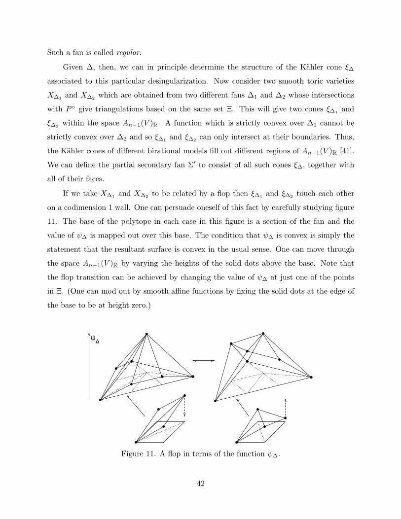
Such a fan is called regular.

Given ∆, then, we can in principle determine the structure of the Kahler cone ξ∆

associated to this particular desingularization. Now consider two smooth toric varieties

X∆1and X∆2

which are obtained from two different fans ∆1 and ∆2 whose intersections

with P ◦ give triangulations based on the same set Ξ. This will give two cones ξ∆1and

ξ∆2within the space An−1(V )R. A function which is strictly convex over ∆1 cannot be

strictly convex over ∆2 and so ξ∆1and ξ∆2

can only intersect at their boundaries. Thus,

the Kahler cones of different birational models fill out different regions of An−1(V )R [41].

We can define the partial secondary fan Σ′ to consist of all such cones ξ∆, together with

all of their faces.

If we take X∆1and X∆2

to be related by a flop then ξ∆1and ξ∆2

touch each other

on a codimension 1 wall. One can persuade oneself of this fact by carefully studying figure

11. The base of the polytope in each case in this figure is a section of the fan and the

value of ψ∆ is mapped out over this base. The condition that ψ∆ is convex is simply the

statement that the resultant surface is convex in the usual sense. One can move through

the space An−1(V )R by varying the heights of the solid dots above the base. Note that

the flop transition can be achieved by changing the value of ψ∆ at just one of the points

in Ξ. (One can mod out by smooth affine functions by fixing the solid dots at the edge of

the base to be at height zero.)

∆ψ

Figure 11. A flop in terms of the function ψ∆.

42

This shows that the smooth resolutions of Vs correspond to cones in An−1(V )R touch-

ing each other along codimension 1 walls if they are related by flops. We now want to

explicitly find these cones. In practice, the authors of [41,42] have given a simple algo-

rithm for carrying out this procedure:

Define an n× (r − 1) matrix A whose columns are the coordinates of the elements of

Ξ in N. Define an integer matrix B as a matrix whose columns span the kernel of A. We

will denote the row vectors of B as bi, i = 1 . . . r − 1. These vectors are vectors in the

lattice An−1(V ).

Each big cone σ ∈ ∆ is specified by its one-dimensional subcones and thus n elements

of Ξ, say ρi, i ∈ I. We can then specify a big cone ξσ in An−1(V )R as the cone which has

one-dimensional edges given by {bj} where j runs over the complement of the set I. We

then describe the cone ξ∆ associated to ∆ as

ξ∆ =⋂

σ∈∆

ξσ. (3.39)

The cones ξ∆ for different resolutions of singularities fit together to form a fan — the

partial secondary fan. As its name suggests this fan is not complete and thus does not

yield a compact moduli space. We will explicitly carry out this procedure for a particular

example in section V.

3.9. Toric Geometry of the Complex Structure Moduli Space

Let us consider the moduli space of complex structures on a hypersurface within a

weighted projective space. We will use the n + 1 homogeneous coordinates [z0, . . . , zn].

If we write down the most general form of the equation defining the hypersurface (i.e.,

include all terms compatible with the weight of each coordinate) we obtain something like

p = a0z0z1 . . . zn + . . .+ aszp0

0 + as+1zp1

1 + . . .+ adznd

d + . . .+ aizni

1

1 zni

2

2 + . . . = 0. (3.40)

Let k be the number of terms in this polynomial. As we vary the complex coefficients ai we

may or may not vary the complex structure of the hypersurface. Some of the variations in

ai give nothing more than reparametrizations of the hypersurface and so cannot affect the

complex structure. (Moreover, sometimes not all of the possible deformations of complex

structure can be achieved by deformations of the above type. This always happens for K3

surfaces for example and can happen in complex dimension 3 if the algebraic variety has

43

not been embedded in a large enough ambient space [22].) A simple reparametrization of

the hypersurface is given by the (C∗)n+1 action

(C∗)n+1 : (z0, z1, . . . , zn) → (α0z0, α1z1, . . . , αnzn), αi ∈ C∗. (3.41)

We will consider the case where the only local deformations18 of the polynomial (3.40)

which fail to give a deformation of complex structure are deformations which amount

to a reparametrization of the form (3.41). One should note that this is quite a strong

requirement and excludes, for example, the quintic hypersurface in P4 which has a group

of reparametrizations isomorphic to Gl(5,C) rather than (C∗)5. Also, if some of the

deformations of complex structure are obstructed in the sense of [22] (as indeed will happen

in our example) then we only recover a lower dimensional subspace of the moduli space.

If we first assume that none of the ai’s vanish then we describe an open subset M0 of

our moduli space of the form (C∗)k/(C∗)n+1 ∼= (C∗)k−n−1. By allowing some of the ai’s

to vanish we can (partially) compactify this space. It would thus appear that our moduli

space is a toric variety.

It turns out that to exhibit mirror symmetry most straight-forwardly we need to

modify the above analysis slightly. Let us impose the condition

a0 = 1. (3.42)

This reduces the (C∗)n+1 invariance to (C∗)n — we have used the other C∗ to rescale the

entire equation, in setting a0 = 1. Now as explained earlier, each monomial in (3.41) is

represented by a point in P in the lattice M . The condition that all reparametrizations

are given by (3.41) may be stated in the form that there are no points from P ∩M in

the interior of codimension one faces on P . It can be seen that the (C∗)n action on any

monomial is given by the coordinates of this point in M . This gives rise to the following

exact sequence

1 −→ exp(2πiNC) −→ (C∗)k−1 −→ M0 −→ 1 (3.43)

which gives another description of M0. The (C∗)k−1 is the space of polynomials with

non-zero coefficients and M0 is the resultant open subset of the moduli space in which no

coefficient vanishes. This open set can then be compactified by adding suitable regions

derived from places where some of the coefficients vanish. Thus we have again arrived at

something resembling a toric variety.

18 Note that we have left open the possibility that there are other, more global deformations

which do not affect the complex structure. These would take the form of discrete symmetries

preserving the equation (3.40). We shall ignore such symmetries for the purposes of this paper;

their effects on the analysis of the moduli space are discussed in detail in [37].

44

4. Mirror Manifolds and Toric Geometry

In the previous section we have given some background on how one realizes certain

families of Calabi-Yau spaces in the formalism of toric geometry. As is clear from that

discussion, many of the detailed properties and desired manipulations of these spaces are

conveniently encoded in combinatorial lattice data. We now describe how aspects of mirror

symmetry can also be formulated using toric methods.

4.1. Toric Approach to Mirror Manifolds

It was originally discovered by S-S. Roan [13] that the mirror manifold construction

of [5] has a simple and natural description in toric geometry. Roan found that when

the orbifolding occurring in [5] was described in toric terms, it led to an identification

between the N lattice of X and the M lattice of its mirror Y . From this, he could

show mathematically that the Hodge numbers of the pairs constructed in [5] satisfy the

appropriate equalities. The results of Roan, therefore, indicate that toric methods provide

the correct mathematical language to discuss mirror symmetry.

After Roan’s work, Batyrev [14] has further pursued the application of toric methods

to mirror symmetry and successfully generalized Roan’s results. Batyrev’s idea is based on

the fact, discussed in section III, that for a Calabi-Yau hypersurface in a toric variety the

polyhedron P in the M lattice contains the data associated with the complex structure de-

formations and the polar polyhedron P ◦ in the N lattice contains data associated with the

Kahler structure. Since mirror symmetry interchanges these data it is natural to suspect

that if X and Y are a mirror pair, and if each has a realization as a toric hypersurface,

then the polyhedron P associated to X , say PX , and its polar P ◦X should be isomorphic to

P ◦Y and PY , respectively. In fact, Batyrev has shown that for any Calabi-Yau hypersurface

X in a toric variety described by the polyhedra P and P ◦ in M and N respectively, if we

construct a new hypersurface Y by interchanging the roles of P and P ◦ then the result is

also Calabi-Yau and furthermore has Hodge numbers consistent with Y being the mirror

of X . This result of Batyrev agrees with that of Roan in the special case of quotients of

Fermat-type hypersurfaces X and Y being related by orbifolding, but goes well beyond

this class of examples. It must be borne in mind, though, that true mirror symmetry

involves much more than these equalities between Hodge numbers. While it seems quite

possible that the new pairs constructed by Batyrev are mirrors, establishing this would

require showing that both members of a proposed pair correspond to isomorphic conformal

theories. This, as yet, has not been done. We therefore confine our attention to the use

of toric methods for those examples in which the latter conformal field theory requirement

has been established — namely those of [5].

45

4.2. Complex Structure vs. Kahler Moduli Space: A Puzzle

In subsections 3.8 and 3.9 we described the Kahler and complex structure moduli

spaces of a Calabi-Yau hypersurface in a toric variety using toric geometry, as these moduli

spaces themselves are toric. If X and Y are a mirror pair, then the Kahler moduli space

of X must be isomorphic to the complex structure moduli space of Y and vice versa. This

statement, however, immediately presents us with the puzzle discussed in subsection 2.5.

Namely, the Kahler moduli space is partitioned into cells with the walls of the partitions

corresponding to singular geometrical configurations in which a curve has been blown

down to a point. From the point of view of toric geometry, these cells correspond to the

different cones in the partial secondary fan of subsection 3.8. The locus of points in the

complex structure moduli space which correspond to singular geometrical configurations,

however, has a very different character. Rather than being real codimension one, and

hence partitioning the moduli space, they are complex codimension one and hence can

generically be avoided when traversing a path between any two points in the moduli space.

How, therefore, can the two spaces of figures 1 and 3 be isomorphic?

There are two possible answers to this question:

1) It might be that only one region of figure 1 has a physical interpretation and, under

mirror symmetry, corresponds to the whole complex structure moduli space. This helps

to resolve the puzzle as we can traverse a nonsingular path between any two points in

a given Kahler region just as we could in the complex structure moduli space. Such a

resolution of this puzzle would imply that flops have no physical interpretation, that the

string somehow picks out one of the many possible resolutions of singularities and that,

unfortunately, topology change in string theory cannot be realized in this manner.

2) The second possible resolution is that all of the regions in figure 1 have a phys-

ical realization and that a generic point on a cell wall (which corresponds under mirror

symmetry to a perfectly smooth complex structure on Y ) although geometrically singular,

is physically smooth. This resolution of the puzzle would therefore imply that flops have

a physical realization and, in fact, would provide us with an operation for changing the

topology of spacetime in a physically smooth manner.

The purpose of [8] and the present work is to present strong evidence that resolution

number two is correct. Let us, therefore, elaborate on this possibility.

We recall from our discussion in section II that the mathematical descriptions we have

given for the complex and Kahler moduli spaces in general are lowest order approximations

46

to the true conformal field theory moduli spaces. Therefore, a more precise statement of

the isomorphism of moduli spaces following from mirror symmetry is: the sector of the

conformal field theory moduli space whose lowest order description is given by the Kahler

moduli space of X is isomorphic to the sector of the conformal field theory moduli space

whose lowest order description is given by the complex structure of Y , and vice versa. Now,

due to certain nonrenormalization theorems [43,44], the complex structure moduli space

actually describes the corresponding sector of conformal field theory moduli space exactly.

Even without such a result, we can always focus on a regime in which the volume of Y is

large (corresponding to a point of large complex structure on X) and hence be able to trust

quantum field theory perturbation theory. The latter assures us that nonsingular choices

for the complex structure of Y yield physically well behaved conformal field theories. On

the other hand, near a wall within the Kahler moduli space of X perturbation theory

becomes an increasingly poor guide to the physics as the volume of certain rational curves

becomes small. Thus, we cannot trust the classical result that the manifold becomes

singular at the wall to necessarily indicate that the physics becomes singular as well.

Resolution number two exploits this possibility to the fullest.

How can we choose between these two possible solutions to the issue we have raised?

There is a very delicate prediction which emerges from solution (2) but not from (1):

solution (2) implies that each point in figure 3 corresponds, under mirror symmetry, to

some point in the complex structure moduli space of Y (we imagine keeping the complex

structure of X and the Kahler structure of Y fixed). Correlation functions calculated in

the two corresponding nonlinear σ-models should therefore be identically equal (if the cor-

responding operators have been normalized identically). Thus, a sensitive test of solution

(2) is to calculate a set of correlation functions at a particular point in each of the cells

of the Kahler moduli space and show that there are corresponding points in the complex

structure moduli space of the mirror such that correlation functions of corresponding ob-

servables (under the identifications following from mirror symmetry) give identical answers.

A specific example of an equality which follows from this reasoning is given in eqn (2.6).

Ideally, to carry out this important test we would understand the precise map between

points in the Kahler moduli space of X to points in the complex structure moduli space of

Y (the “mirror map”) and also the precise map between observables in the theory based on

X to those of the theory based on Y . In reality, though, we can carry out this test without

such precise knowledge of the mirror map, so long as we carefully choose the points in

the Kahler moduli space around which we do our calculation. Namely, if we choose the

47

large radius points in each of the Kahler cells (corresponding to large radius Calabi-Yau

manifolds which are birationally equivalent but topologically distinct) then toric geometry,

as we shall now discuss, provides us with a tool for locating the corresponding “large

complex structure” points on the mirror and also for mapping between observables in

the two models. We emphasize that solution (2), in contrast with (1), implies that the

equalities of correlation functions we have mentioned follows for any and all choices of

points in the partially enlarged Kahler moduli space (that is, including all of the bordering

regions we have been discussing). Our choice to work near large radius points is therefore

one of convenience (calculations are easier there) and in no way compromises or yields an

approximate result.

4.3. Asymptotic Mirror Symmetry and The Monomial-Divisor Mirror Map

Given a specific manifoldX at some large radius limit our aim is to determine precisely

which “large complex structure limit” its mirror partner Y has attained. This can be

achieved if we can find the mirror map between the complexified Kahler moduli space

of X and the moduli space of complex structures of Y . We have already seen in the

preceding sections that in the cases we are considering, both these spaces are isomorphic

to toric varieties which are (compactifications of) (C∗)Ξ/(C∗)n.

In the case of the moduli space of complexified Kahler forms on X , Ξ represented the

set of toric divisors on X . The (C∗)n action represents linear equivalence and is determined

by the arrangement of the points corresponding to Ξ in the lattice N . In the case of the

moduli space of complex structures on Y , using the results of subsections 3.9 and 4.1, Ξ

now represents the set of monomials in the defining equation for Y (with the exception

of the a0 term) and the (C∗)n action represents reparametrizations determined by the

arrangement of the points of Ξ in the lattice N .

We have thus arrived at a natural proposal for the mirror map, namely to simply

identify the divisors of X given by Ξ ⊂ N with the monomials of Y also given by Ξ ⊂ N .

The induced map between the moduli spaces is called the monomial-divisor map, and it is

unique up to symmetries of the point set Ξ ⊂ N . However, it turns out that although this

proposal for a mirror map has the correct asymptotic behavior near the large radius limit

points, it unfortunately differs from the actual mirror map away from large radius limits.

More will be explained concerning this point in [45]. This problem was also observed from a

different view-point in [12] where extra small-scale instantons appeared in the “A-model”.

Fortunately our only concern in this paper is with large radius limits and so we may take

48

this naıve identification of the two moduli spaces as an approximation of the true mirror

map which is adequate for our purposes. For a more mathematical discussion of these

points see [37].

In order to determine the large radius limits of X we now consider compactifications

of (C∗)Ξ/(C∗)n. In terms of the Kahler form, J , on X we are studying a limit in which

e2πi(B+iJ) → 0 by taking J → ∞ inside the Kahler cone, ξX , of X .19 In the language of

toric geometry, this point added to the moduli space is given by the cone ξX ⊂ An−1(V )R.

In this way we determine a compactification of the space of complexified Kahler forms on

X which includes all large radius limits. It is the toric variety given by the Kahler cone of

X and its neighbours with respect to the lattice An−1(V ).

A large radius limit of X can now be translated into a large complex structure limit

of Y . The fact that J remains within ξX dictates the relative growth of the coefficients

ai of the monomials as they are taken to ∞ (or 0). Any path in the moduli space with

the property that the coefficients of the corresponding family of hypersurfaces obey these

growth properties will approach the large complex structure limit point specified by ξX .

We will now demonstrate how this can be done explicitly by an example.

5. An Example

In the previous section we described the application of toric geometry to mirror sym-

metry and showed how these methods could be used to verify or disprove our claim that

the mathematical operation of flopping rational curves — which can result in the change

of topology of the underlying space — is physically realized and perfectly well behaved.

We will now carry out this procedure in a specific example. We emphasize that although

we work in a specific example of a particular Calabi-Yau and its mirror (chosen for their

relative calculational simplicity) our results are certainly general. Namely, the operation

of flopping is a local operation which is insensitive to global properties of the space. If we

can show that flopping is physically sensible and realizable in a specific example, it will

certainly have these desired properties in any other example as the local description and

hence physical phenomenon will be the same.

19 More precisely, ξX represents that part of the Kahler cone of X which comes from the ambient

space V — it is in reality the Kahler cone of V that we study.

49

5.1. A Mirror Pair of Calabi-Yau Spaces

We require an example sufficiently complicated to exhibit flops. We also imposed a

condition in subsection 3.9 to obtain a toric structure for the moduli space. That is, we

require the group of reparametrizations of the hypersurface equation to be (C∗)5. The

following example is one of the simplest cases meeting these requirements.

Let Xs be a hypersurface in V ∼= P4{6,6,3,2,1} given by

f = z30 + z3

1 + z62 + z9

3 + z184 = 0. (5.1)

This space has quotient singularities inherited from P4{6,6,3,2,1}. Namely, there are two

curves of Z2 and Z3 singularities respectively and these intersect at three points which

locally have the form of Z6 singularities. These singularities are the same as the singu-

larities studied in [18]. Any blow-up of these singularities to give a smooth X gives an

exceptional divisor with 6 irreducible components, thus h1,1(X) = 7. When one resolves

the singularities in P4{6,6,3,2,1} one only obtains an exceptional set with 4 components. One

of these components intersects X in regions around the 3 former Z6 quotient singularities.

Thus 3 elements of H2(X) are being produced by a single element of H2(V ).

In terms of Kahler form moduli space one can picture this as follows. Each of the

three Z6 quotient singularities contributes a component of the exceptional divisor. As far

as the Kahler cone of X is concerned the volume of these three divisors can be varied

independently. If we wish to describe the Kahler form on X in terms of a Kahler form on

V however, these three volumes had better be the same since they all come from one class

in H2(V ). Thus we are restricting to the part of the moduli space of Kahler forms on X

where these three volumes are equal. An important point to notice is that even though we

are ignoring some directions in moduli space, we can still get to a large radius limit where

all components of the exceptional divisor in X are large.

The toric variety P4{6,6,3,2,1} is given by complete fan around O whose one dimensional

cones pass through the points

α5 = (1, 0, 0, 0)

α6 = (0, 1, 0, 0)

α7 = (0, 0, 1, 0)

α8 = (0, 0, 0, 1)

α9 = (−6,−6,−3,−2).

(5.2)

50

This data uniquely specifies the fan in this case. (The reason for the curious numbering

scheme will become apparent.) This fan is comprised of five big cones most of which have

volume > 1. For example, the cone subtended by {α5, α7, α8, α9} has volume 6. The sum

of the volumes of these 5 cones is 18 and thus we need to subdivide these 5 cones into 18

cones to obtain a smooth Calabi-Yau hypersurface. The extra points on the boundary of

P ◦ which are available to help us do this are

α1 = (−3,−3,−1,−1)

α2 = (−2,−2,−1, 0)

α3 = (−4,−4,−2,−1)

α4 = (−1,−1, 0, 0).

(5.3)

Note that, as required, none of these points lies in the interior of a codimension one face of

P ◦. Any complete fan ∆ of simplicial cones having all of the lines through {α1, . . . , α9} as

its set of one-dimensional cones will consist of 18 big cones and specify a smooth Calabi-Yau

hypersurface, but the data {α1, . . . , α9} does not uniquely specify this fan.

A little work shows that there are 5 possible fans consistent with this data, all of

which are regular. That is, all 5 possible toric resolutions of P4{6,6,3,2,1} are Kahler. We

can uniquely specify the fan ∆ just by specifying the resulting triangulation of the face

{α7, α8, α9}. The possibilities are shown in figure 12 and in figure 13 the three-dimensional

simplices are shown for resolution ∆1.

α2

α2

α2

α2

α2

α3

α3

α3

α3

α3

α1

α1

α1

α1

α1

α7

α7

α7

α7

α7

α9

α9

α9

α9

α9

α8

α8

α8

α8

α8

α1α

4

α3α

4

α2α

4

α4

α4

α4

α4

α4

1 2

3 4 5

α1α

3

∆ ∆

∆ ∆∆

Figure 12. The five smooth models.

51

α

α α

α α

α α

α

α α

α

α

α α α α

α α

α αα α

α α α α

α α α

αα

1 1

2 23 3

4 4

1

23

7

9

5

8

7

6

98

5

6

9 8

5

6

97

5

6

78

Figure 13. The tetrahedra in resolution ∆1.

To obtain Y as a mirror of X , we divide X by the largest “phase” symmetry consistent

with the trivial canonical bundle condition [5]. This is given by the following generators:

[z0, z1, z2, z3, z4] → [ωz0, z1, z2, z3, ω2z4]

[z0, z1, z2, z3, z4] → [z0, ωz1, z2, z3, ω2z4]

[z0, z1, z2, z3, z4] → [z0, z1, ωz2, z3, ω2z4],

(5.4)

where ω = exp(2πi/3). This produces a whole host of quotient singularities but since we

are only concerned with the complex structure of Y we can ignore this fact.

In light of the results of [12] and the discussion in section VI, we should actually be

more careful in our use of language here. To be more precise, given the Landau-Ginzburg

model XLG whose superpotential is specified in (5.1), we can construct another Landau-

Ginzburg theory YLG as the orbifold ofXLG by the group generated by (5.4) and having the

same superpotential (5.1). YLG is the mirror of XLG. Up to now however, we had assumed

that X and Y were smooth Calabi-Yau manifolds. As shown in [12] and as will become

clear in section VI, the smooth Calabi-Yau manifolds occupy a different region of the same

moduli space as the Landau-Ginzburg theory. Thus if we deform both of our mirror pair

XLG and YLG, then we can obtain two smooth mirror manifolds X and Y . If we wanted to

compare all correlation functions of the conformal field theories of X and Y then we would

have to do this. All we are going to do in this section however is to compare information

concerning the Kahler sector of X with the complex structure sector of Y . Information

concerned with the complex structure of Y as a smooth manifold is isomorphic to that of

52

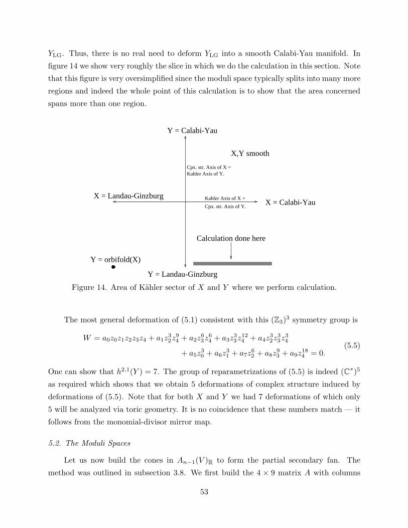
YLG. Thus, there is no real need to deform YLG into a smooth Calabi-Yau manifold. In

figure 14 we show very roughly the slice in which we do the calculation in this section. Note

that this figure is very oversimplified since the moduli space typically splits into many more

regions and indeed the whole point of this calculation is to show that the area concerned

spans more than one region.

X = Landau-Ginzburg

Y = Calabi-Yau

Y = Landau-Ginzburg

Y = orbifold(X)

X,Y smooth

Calculation done here

X = Calabi-YauKahler Axis of X =

Kahler Axis of Y.Cpx. str. Axis of X =

Cpx. str. Axis of Y.

Figure 14. Area of Kahler sector of X and Y where we perform calculation.

The most general deformation of (5.1) consistent with this (Z3)3 symmetry group is

W = a0z0z1z2z3z4 + a1z32z

94 + a2z

63z

64 + a3z

33z

124 + a4z

32z

33z

34

+ a5z30 + a6z

31 + a7z

62 + a8z

93 + a9z

184 = 0.

(5.5)

One can show that h2,1(Y ) = 7. The group of reparametrizations of (5.5) is indeed (C∗)5

as required which shows that we obtain 5 deformations of complex structure induced by

deformations of (5.5). Note that for both X and Y we had 7 deformations of which only

5 will be analyzed via toric geometry. It is no coincidence that these numbers match — it

follows from the monomial-divisor mirror map.

5.2. The Moduli Spaces

Let us now build the cones in An−1(V )R to form the partial secondary fan. The

method was outlined in subsection 3.8. We first build the 4 × 9 matrix A with columns

53

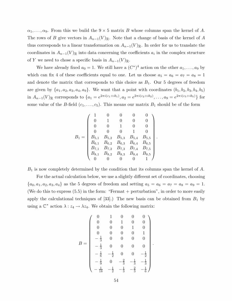
α1, . . . , α9. From this we build the 9 × 5 matrix B whose columns span the kernel of A.

The rows of B give vectors in An−1(V )R. Note that a change of basis of the kernel of A

thus corresponds to a linear transformation on An−1(V )R. In order for us to translate the

coordinates in An−1(V )R into data concerning the coefficients ai in the complex structure

of Y we need to chose a specific basis in An−1(V )R.

We have already fixed a0 = 1. We still have a (C∗)4 action on the other a1, . . . , a9 by

which can fix 4 of these coefficients equal to one. Let us choose a5 = a6 = a7 = a8 = 1

and denote the matrix that corresponds to this choice as B1. Our 5 degrees of freedom

are given by {a1, a2, a3, a4, a9}. We want that a point with coordinates (b1, b2, b3, b4, b5)

in An−1(V )R corresponds to {a1 = e2πi(c1+ib1), a2 = e2πi(c2+ib2), . . . , a9 = e2πi(c5+ib5)} for

some value of the B-field (c1, . . . , c5). This means our matrix B1 should be of the form

B1 =

1 0 0 0 00 1 0 0 00 0 1 0 00 0 0 1 0

B5,1 B5,2 B5,3 B5,4 B5,5

B6,1 B6,2 B6,3 B6,4 B6,5

B7,1 B7,2 B7,3 B7,4 B7,5

B8,1 B8,2 B8,3 B8,4 B8,5

0 0 0 0 1

.

B1 is now completely determined by the condition that its columns span the kernel of A.

For the actual calculation below, we use a slightly different set of coordinates, choosing

{a0, a1, a2, a3, a4} as the 5 degrees of freedom and setting a5 = a6 = a7 = a8 = a9 = 1.

(We do this to express (5.5) in the form: “Fermat + perturbation”, in order to more easily

apply the calculational techniques of [33].) The new basis can be obtained from B1 by

using a C∗ action λ : z4 → λz4. We obtain the following matrix:

B =

0 1 0 0 00 0 1 0 00 0 0 1 00 0 0 0 1− 1

3 0 0 0 0

− 13 0 0 0 0

− 16

−12

0 0 −12

− 19 0 −2

3 −13 −1

3

− 118 −1

2 −13 −2

3 −16

.

54

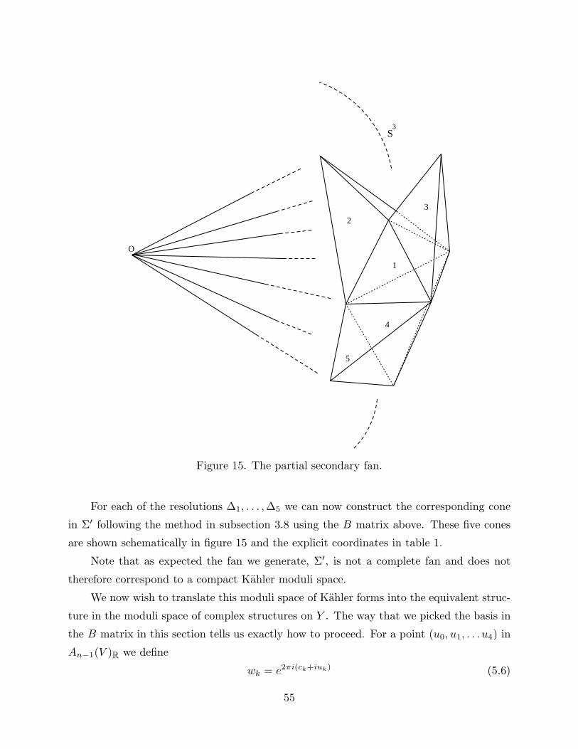
S3

1

2

3

4

5

O

Figure 15. The partial secondary fan.

For each of the resolutions ∆1, . . . ,∆5 we can now construct the corresponding cone

in Σ′ following the method in subsection 3.8 using the B matrix above. These five cones

are shown schematically in figure 15 and the explicit coordinates in table 1.

Note that as expected the fan we generate, Σ′, is not a complete fan and does not

therefore correspond to a compact Kahler moduli space.

We now wish to translate this moduli space of Kahler forms into the equivalent struc-

ture in the moduli space of complex structures on Y . The way that we picked the basis in

the B matrix in this section tells us exactly how to proceed. For a point (u0, u1, . . . u4) in

An−1(V )R we define

wk = e2πi(ck+iuk) (5.6)

55

v1 (− 1

3, 0, 0, 0, 0)

v2 (− 7

18,− 1

2,− 1

3,− 2

3,− 1

6)

v3 (− 1

6,− 1

2, 0, 0,− 1

2)

v4 (− 2

9, 0,− 1

3,− 2

3,− 2

3)

v5 (− 1

9, 0,− 2

3,− 1

3,− 1

3)

Table 1a: Generators for first cone

Resolution Generators

∆1 v1, v2, v3, v4, v5

∆2 v1, v1 − v2 + v3 + v4, v3, v4, v5

∆3 v1, v2, v2 − v3 + v4, v4, v5

∆4 v1, v2, v3, v2 + v3 − v4 + v5, v5

∆5 v1, v2, v3, v2 + v3 − v4 + v5,v3 + (v2 + v3 − v4 + v5) − v5

Table 1b: Generators for all cones

for any real ck’s. This is then mapped to (5.5) by

ai = w−1i , i = 0, . . . , 4

ai = 1, i = 5, . . . , 9.(5.7)

5.3. Results

We have now done enough work to achieve one of our original goals, i.e., given a

specific topology of X we can determine which direction in the moduli space of Y should

be taken to find the intersection numbers of X . All we do is is take a direction going out

to infinity within the interior of the corresponding cone in Σ′ and convert this limit by

(5.6).

Just as was done in [33], it is easiest to compare intersection numbers from the two

methods by computing ratios which would be invariant under rescaling of the monomials

in (5.5). There are many such ratios although we will only consider 4 here for brevity.

As explained earlier, all intersection numbers are determined by the data in ∆ although

we only outlined how to calculate the intersection number of three homologically distinct

cycles. For the exact method of determining self-intersections we refer to [46] or the method

56

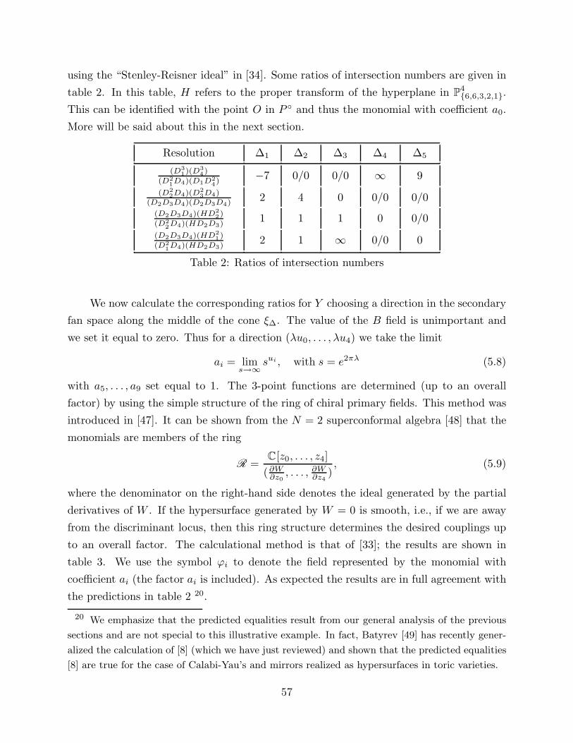
using the “Stenley-Reisner ideal” in [34]. Some ratios of intersection numbers are given in

table 2. In this table, H refers to the proper transform of the hyperplane in P4{6,6,3,2,1}.

This can be identified with the point O in P ◦ and thus the monomial with coefficient a0.

More will be said about this in the next section.

Resolution ∆1 ∆2 ∆3 ∆4 ∆5

(D31)(D3

4)

(D21D4)(D1D2

4)

−7 0/0 0/0 ∞ 9

(D22D4)(D

23D4)

(D2D3D4)(D2D3D4)2 4 0 0/0 0/0

(D2D3D4)(HD22)

(D22D4)(HD2D3)

1 1 1 0 0/0

(D2D3D4)(HD21)

(D21D4)(HD2D3)

2 1 ∞ 0/0 0

Table 2: Ratios of intersection numbers

We now calculate the corresponding ratios for Y choosing a direction in the secondary

fan space along the middle of the cone ξ∆. The value of the B field is unimportant and

we set it equal to zero. Thus for a direction (λu0, . . . , λu4) we take the limit

ai = lims→∞

sui , with s = e2πλ (5.8)

with a5, . . . , a9 set equal to 1. The 3-point functions are determined (up to an overall

factor) by using the simple structure of the ring of chiral primary fields. This method was

introduced in [47]. It can be shown from the N = 2 superconformal algebra [48] that the

monomials are members of the ring

R =C[z0, . . . , z4]

(∂W∂z0

, . . . , ∂W∂z4

), (5.9)

where the denominator on the right-hand side denotes the ideal generated by the partial

derivatives of W . If the hypersurface generated by W = 0 is smooth, i.e., if we are away

from the discriminant locus, then this ring structure determines the desired couplings up

to an overall factor. The calculational method is that of [33]; the results are shown in

table 3. We use the symbol ϕi to denote the field represented by the monomial with

coefficient ai (the factor ai is included). As expected the results are in full agreement with

the predictions in table 2 20.

20 We emphasize that the predicted equalities result from our general analysis of the previous

sections and are not special to this illustrative example. In fact, Batyrev [49] has recently gener-

alized the calculation of [8] (which we have just reviewed) and shown that the predicted equalities

[8] are true for the case of Calabi-Yau’s and mirrors realized as hypersurfaces in toric varieties.

57

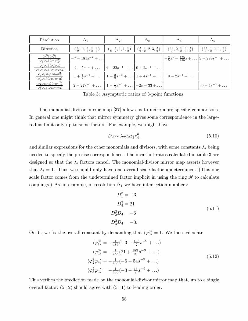
Resolution ∆1 ∆2 ∆3 ∆4 ∆5

Direction ( 11

9, 1,

4

3,

5

3,

5

3) ( 7

6,

1

2, 1, 1,

5

2) ( 3

2,

1

2, 2, 3,

3

2) ( 13

9, 2,

5

3,

4

3,

4

3) ( 11

6,

7

2, 1, 1,

3

2)

〈ϕ31〉〈ϕ3

4〉

〈ϕ21

ϕ4〉〈ϕ1ϕ24〉

−7 − 181s−1 + . . . −

2

5s2−

129

250s + . . . 9 + 289s

−1 + . . .

〈ϕ22

ϕ4〉〈ϕ23

ϕ4〉

〈ϕ2ϕ3ϕ4〉〈ϕ2ϕ3ϕ4〉2 − 5s

−1 + . . . 4 − 22s−1 + . . . 0 + 2s

−1 + . . .

〈ϕ2ϕ3ϕ4〉〈ϕ0ϕ22〉

〈ϕ22

ϕ4〉〈ϕ0ϕ2ϕ3〉1 + 1

2s−1 + . . . 1 + 3

2s−2 + . . . 1 + 4s

−1 + . . . 0 − 2s−1 + . . .

〈ϕ2ϕ3ϕ4〉〈ϕ0ϕ21〉

〈ϕ21

ϕ4〉〈ϕ0ϕ2ϕ3〉2 + 27s

−1 + . . . 1 −

1

2s−1 + . . . −2s − 33 + . . . 0 + 4s

−2 + . . .

Table 3: Asymptotic ratios of 3-point functions

The monomial-divisor mirror map [37] allows us to make more specific comparisons.

In general one might think that mirror symmetry gives some correspondence in the large-

radius limit only up to some factors. For example, we might have

D2 ∼ λ2a2z63z

64 , (5.10)

and similar expressions for the other monomials and divisors, with some constants λi being

needed to specify the precise correspondence. The invariant ratios calculated in table 3 are

designed so that the λi factors cancel. The monomial-divisor mirror map asserts however

that λi = 1. Thus we should only have one overall scale factor undetermined. (This one

scale factor comes from the undetermined factor implicit in using the ring R to calculate

couplings.) As an example, in resolution ∆1 we have intersection numbers:

D31 = −3

D34 = 21

D22D4 = −6

D23D4 = −3.

(5.11)

On Y , we fix the overall constant by demanding that 〈ϕ30〉 = 1. We then calculate

〈ϕ31〉 = − 1

486(−3 − 1952 s−9 + . . .)

〈ϕ34〉 = − 1

486(21 + 183

2s−9 + . . .)

〈ϕ22ϕ4〉 = − 1

486(−6 − 54s−9 + . . .)

〈ϕ23ϕ4〉 = − 1

486(−3 − 452 s

−9 + . . .)

(5.12)

This verifies the prediction made by the monomial-divisor mirror map that, up to a single

overall factor, (5.12) should agree with (5.11) to leading order.

58

5.4. Discussion

Let us recapitulate what we learn from this example. In subsection 4.2 we presented

a puzzle regarding the apparent asymmetry between complex and Kahler moduli spaces.

We presented the two possible resolutions of this puzzle and a method of adjudicating

between them. In the context of the present example, we have explicitly carried out

this distinguishing test and shown that the second resolution of subsection 4.2 is verified.

Namely, under mirror symmetry (part of) the complex structure moduli space of Y is

isomorphic to the (partially) enlarged Kahler moduli space of X (and vice versa) 21. We

have shown this by explicitly verifying that distinct points in the complex structure moduli

space of Y are mapped to points in distinct regions in the (partially) enlarged Kahler

moduli space of X .

Although we have carried out this analysis in the context of a specific example, we

want to emphasize that our picture of the enlarged Kahler moduli space, its toric geomet-

ric description and its relation to the complex structure moduli space of the mirror, as

presented in previous sections, is completely general. The present example has served as

an explicit verification.

6. The Fully Enlarged Kahler Moduli Space

The analysis of the moduli spaces thus far leaves unanswered the following interesting

question. As the fan Σ′ is not complete we can inquire as to what happens if we take

a limiting complex structure on Y given by a direction not contained in Σ′. Up to this

point, we would be unable to give a corresponding mirror space X for such a limit. The

reader might also have noticed the rather asymmetric way we treated the point O in P ◦

and thus the monomial corresponding to a0. As we will see, a more symmetric treatment

of the polytope P ◦ will open up the other regions of the Kahler moduli space and yield

a rich structure. It will turn out that these other regions of moduli space will not have

interpretations as smooth Calabi-Yau manifolds and are thus missed by classical σ-model

ideas. Thus this rich structure is one example of the differences between classical and

quantum geometry.

21 In the next section we will consider the fully enlarged Kahler moduli space and show it to

be isomorphic to the full moduli space of complex structures on Y .

59

First let us reconsider the moduli space of complex structures on a hypersurface within

a weighted projective space. In (3.42) we artificially singled out a0 amongst the coefficients

so that we could reduce the (C∗)n+1 action on the homogeneous coordinates to the required

(C∗)n action to obtain a toric variety for the moduli space compatible with the moduli

space of Kahler forms. As explained earlier, each monomial in (3.41) is represented by a

point in P in the lattice M . Let us introduce a lattice M+ of dimension n+1 obtained by

adding one further generator to the generators of M in an orthogonal direction. Thus P

lies in a hyperplane within M+R

. It can be seen that the (C∗)n+1 action on any monomial

is given by the coordinates of this point in M+. This now gives rise to the following exact

sequence

1 −→ exp(2πiM+∗C

) −→ (C∗)k −→ M0 −→ 1. (6.1)

The (C∗)k is the space of polynomials with non-zero coefficients and M0 is the resultant

open subset of the moduli space. This process is of course entirely equivalent to (3.43).

The difference now comes when we compactify this space. The fact that we can now let

a0 → 0 opens up new possibilities reflected by the fact that some of the dimensions of the

vector spaces in the above exact sequence have increased.

Now let us reconsider the space of Kahler forms on a toric variety specified by a fan

∆, describing it in terms of the triangulation of P ◦ determined by ∆. Consider a simplex

in n-dimensions with n+ 1 vertices. If we attach a real number to each vertex then have

specified an affine function on the simplex whose value at each vertex is the number we

specify. Indeed the space of affine functions on this simplex can be given by the space Rn+1

of numbers on the vertices. Consider now attaching a real number to each point in the

set A = P ◦ ∩N . This can be taken to define a continuous (but not necessarily smooth)

function Ψ∆ : NR → R which is a smooth affine function in each simplex. The space of

all such functions is isomorphic to Rr, where r is the number of points in P ◦ ∩N .

We have previously described the Kahler forms on V∆ in terms of functions which

are linear on each cone; we now modify this to a description in terms of functions which

are affine on each simplex. The space of smooth linear functions on NR is the dual vector

space N∗R. We can go to the space of smooth affine functions if we add an extra dimension

to get N+∗R

. We can then write down the following exact sequence

0 −→ N+∗R

−→ Rr −→ An−1(V )R −→ 0, (6.2)

60

where the space Rr is interpreted as the space of functions Ψ∆. The Kahler forms are now

specified by a convexity condition. In fact, we have the following analogue of (3.37):

Space of Kahler forms on V∆∼=

Space of strictly convex Ψ∆

Space of smooth Ψ∆(6.3)

where this time we take Ψ∆ from the space Rr of continuous functions which are affine on

each simplex. of Kahler forms on XΣ will be a subspace of An−1(V )R.

We can now repeat the construction of cones in the partial secondary fan in a slightly

extended version of the algorithm in subsection 3.8: Extend the coordinates of the r points

in A to coordinates in the (n + 1)-dimensional space N+R

simply by adding a “1” in the

(n+ 1)th place and take A+ to be the (n+ 1)× r matrix of these column vectors. Denote

the columns of A+ as ai, i = 1 . . . r. Let the kernel of A+ be spanned by the columns of

the n × (r − n − 1) matrix B+. Let b+i , i = 1 . . . r be the resulting vectors in An+1(V )R

whose coordinates are given by the rows of B+.

Now each maximal simplicial cone, σ ∈ ∆, is specified by n + 1 elements of A , one

of the elements being O. Thus when we consider the complimentary set of bj ’s, we never

include b0. Thus we build precisely the same cone ξ∆ in the partial secondary fan as we

did in subsection 3.8.

We know that this does not fill out the whole of the secondary fan. It is known however

that if we consider the set of cones corresponding to all possible triangulations based in A

consistent with the convexity of Ψ∆ then these do indeed fill out the whole of An−1(V )R

[42]. One should note that by all possible triangulations, we include triangulations which

may ignore some of the points in A (although not the points on the vertices of P ◦). The

process of ignoring an interior point and the way it relates to Ψ∆ is shown in figure 16

(cp. the flop shown in figure 11). We will refer to removing a point in this way as a

star-unsubdivision (since the inverse process is often known as a star-subdivision). Star

unsubdivisions at an arbitrary point are not necessarily allowed since the resultant network

might not be a triangulation but when they are allowed, they correspond to a codimension

1 wall of two neighbouring cones in much the same way as a flop did.

In general not all possible triangulations based in A admit a strictly convex function.

A toric variety from such a triangulation does not admit a Kahler metric [41]. It turns

out that in our example there are no such triangulations. In more complicated examples

however one might have the situation where a smooth Kahler manifold could be flopped

61

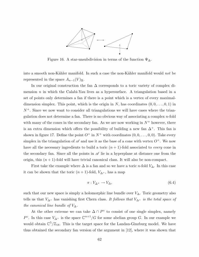
Figure 16. A star-unsubdivision in terms of the function Ψ∆.

into a smooth non-Kahler manifold. In such a case the non-Kahler manifold would not be

represented in the space An−1(V )R.

In our original construction the fan ∆ corresponds to a toric variety of complex di-

mension n in which the Calabi-Yau lives as a hypersurface. A triangulation based in a

set of points only determines a fan if there is a point which is a vertex of every maximal-

dimension simplex. This point, which is the origin in N , has coordinates (0, 0, . . . , 0, 1) in

N+. Since we now want to consider all triangulations we will have cases where the trian-

gulation does not determine a fan. There is no obvious way of associating a complex n-fold

with many of the cones in the secondary fan. As we are now working in N+ however, there

is an extra dimension which offers the possibility of building a new fan ∆+. This fan is

shown in figure 17. Define the point O+ in N+ with coordinates (0, 0, . . . , 0, 0). Take every

simplex in the triangulation of A and use it as the base of a cone with vertex O+. We now

have all the necessary ingredients to build a toric (n+ 1)-fold associated to every cone in

the secondary fan. Since all the points in A lie in a hyperplane at distance one from the

origin, this (n+ 1)-fold will have trivial canonical class. It will also be non-compact.

First take the example where ∆ is a fan and so we have a toric n-fold V∆. In this case

it can be shown that the toric (n+ 1)-fold, V∆+ , has a map

π : V∆+ → V∆, (6.4)

such that our new space is simply a holomorphic line bundle over V∆. Toric geometry also

tells us that V∆+ has vanishing first Chern class. It follows that V∆+ is the total space of

the canonical line bundle of V∆.

At the other extreme we can take ∆ ∩ P ◦ to consist of one single simplex, namely

P ◦. In this case V∆+ is the space Cn+1/G for some abelian group G. In our example we

would obtain C5/Z18. This is the target space for the Landau-Ginzburg model. We have

thus obtained the secondary fan version of the argument in [12], where it was shown that

62

+

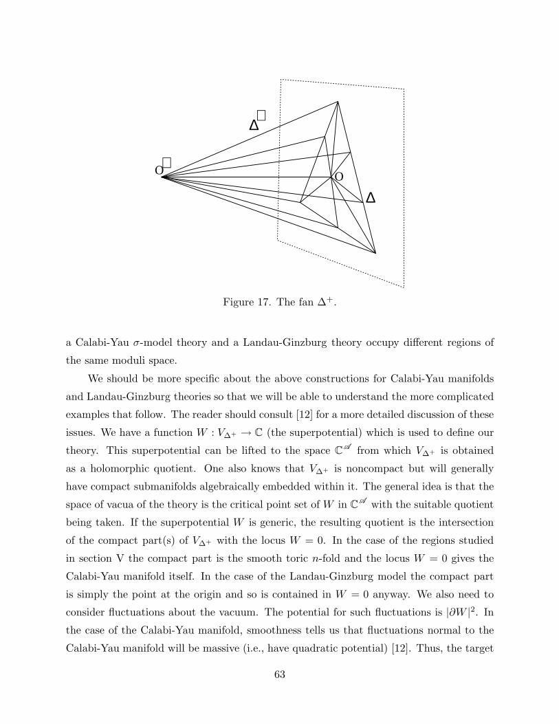
O+O

∆

∆

Figure 17. The fan ∆+.

a Calabi-Yau σ-model theory and a Landau-Ginzburg theory occupy different regions of

the same moduli space.

We should be more specific about the above constructions for Calabi-Yau manifolds

and Landau-Ginzburg theories so that we will be able to understand the more complicated

examples that follow. The reader should consult [12] for a more detailed discussion of these

issues. We have a function W : V∆+ → C (the superpotential) which is used to define our

theory. This superpotential can be lifted to the space CA from which V∆+ is obtained

as a holomorphic quotient. One also knows that V∆+ is noncompact but will generally

have compact submanifolds algebraically embedded within it. The general idea is that the

space of vacua of the theory is the critical point set of W in CA with the suitable quotient

being taken. If the superpotential W is generic, the resulting quotient is the intersection

of the compact part(s) of V∆+ with the locus W = 0. In the case of the regions studied

in section V the compact part is the smooth toric n-fold and the locus W = 0 gives the

Calabi-Yau manifold itself. In the case of the Landau-Ginzburg model the compact part

is simply the point at the origin and so is contained in W = 0 anyway. We also need to

consider fluctuations about the vacuum. The potential for such fluctuations is |∂W |2. In

the case of the Calabi-Yau manifold, smoothness tells us that fluctuations normal to the

Calabi-Yau manifold will be massive (i.e., have quadratic potential) [12]. Thus, the target

63

space is precisely the Calabi-Yau manifold. In the case of the Landau-Ginzburg theory

these fluctuations are massless and are analyzed in the usual way from the superpotential

W .

In addition to σ-models and Landau-Ginzburg theories, there are many other possi-

bilities. In our example, the secondary fan is divided up into 100 cones. That is, there

are 100 different triangulations with vertices in the point set P ◦ ∩ N . Five of these give

smooth Calabi-Yau manifolds and one of these is the Landau-Ginzburg theory. There are

94 other regions to explain!

Let us begin by analyzing the structure of the singularities of V∆+ . In our example,

for every cone in the secondary fan the corresponding ∆+ turns out to be simplicial. Thus,

each cone σ spanning p dimensions in ∆+ is defined by the coordinates of the p vertices of

the simplex σ ∩NR at the base of the cone. The volume of that cone is then the volume

of the polyhedron spanned by O+ and that simplex. Volumes are normalized so that the

unit simplex in Rp = span(σ) (with respect to the lattice N ∩ Rp) has volume 1. (If

we had normalized to make the unit cube have volume 1, as is perhaps more common,

then we would have needed to multiply by p! to obtain this “simplicial” volume.) The

cone represents a smooth part of the toric variety iff this volume is 1. That is, if the

volume of a p-cone is greater than 1 then it represents a singularity along a (n + 1 − p)-

dimensional subvariety of V∆+ . The fact that each cone is a cone over a simplex tells us

that the singularities in question are quotient singularities. That is, a p-cone of volume

v represents a quotient singularity locally of the form Cp/G where G has order v. This

gives the general statement about the correspondence between Landau-Ginzburg models

and Calabi-Yau manifolds. The minimal triangulation based in P ◦ ∩ N consisting of the

single simplex P ◦ is a target space of the form Cn+1/G whereas a maximal triangulation

consisting of |G| (n+ 1)-cones gives a smooth manifold.

Consider now taking a triangulation corresponding to a smooth Calabi-Yau manifold

and star unsubdividing at a point such that O is still a vertex of each simplex of the

triangulation. The (n + 1)-dimensional toric variety V∆+ can still be thought of as the

canonical sheaf of V∆ but now V∆ has acquired quotient singularities. That is, V∆ is an

orbifold22. This leads to a rather striking conclusion as follows. Geometrically speaking,

the orbifolds that arise in the subject of superstring compactification can just be thought of

as special cases of Calabi-Yau manifolds. Any quotient singularity arising from an abelian

22 By “orbifold” we mean a space whose only singularities are locally quotient singularities.

64

group action in three dimensions preserving the holomorphic 3-form can be resolved to

give a smooth Calabi-Yau manifold. In this sense orbifolds appear to live within the walls

of the Kahler cone of a Calabi-Yau manifold. The reverse process to resolution, i.e., the

blowing-down of a divisor within the Calabi-Yau manifold, appears as a path beginning

in the interior of the Kahler cone and ending on the boundary. In this “classical” setting

Calabi-Yau manifolds are more general than orbifolds in the sense that they occupy a

larger dimensional region of moduli space than do orbifolds. In the light of our preceding

discussion it appears that within quantum algebraic geometry one has to modify this

viewpoint. Orbifolds now appear to occupy a region of moduli space equal in dimension

to that of the Calabi-Yau manifold. One should think of orbifolds as not living within the

walls of the Kahler cone of a smooth Calabi-Yau manifold but occupying their own Kahler

cone on the other side of the wall!

In our example 27 of the regions correspond to orbifolds. The possible singularities

encountered are Z2, Z3, Z2 × Z2, Z4 and Z6 quotients.

In these orbifold regions as well as in the smooth Calabi-Yau region, the space V∆+ may

be thought of as a bundle (in some generalized sense to include singularities) over a compact

space. This also holds for Landau-Ginzburg theory. In the case of the Landau-Ginzburg

theory this compact space is a point and in the Calabi-Yau manifold and orbifold cases

this space is a toric d-fold. The other 67 regions of the secondary fan correspond to spaces

intermediate between these. The dimension of the compact space may be determined as

follows. Within the any particular triangulation based in P ◦∩N we may look for complete

fans. Any complete fan spanning Rp corresponds to a toric p-fold. Thus, the maximal p

for which a complete fan can be found will give us the dimension of the complex space.

The resultant space is not necessarily irreducible however.

Figure 18 shows examples of spaces of intermediate dimension in the case d = 2. In

example (a) there is no complete fan of dimension 2 in NR but there is the fan as shown of

dimension 1. Thus the dimension of the compact part of the toric variety has gone down

by 1 from the smooth Calabi-Yau case. In figure (b) there is a dimension 2 fan (shown as

∆2) but not all cones are elements of this fan. Another fan, ∆1 is required to complete the

triangulation. This should be interpreted as follows: ∆1 represents a 1-dimensional space

and ∆2 represents a 2-dimensional space. They intersect at a point since they share one

2-dimensional cone. Example (a) is irreducible but (b) is reducible into two irreducible

components.

65

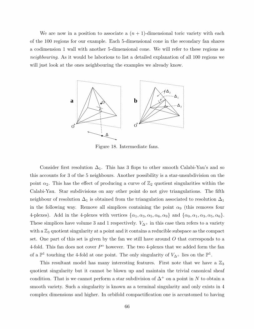
We are now in a position to associate a (n + 1)-dimensional toric variety with each

of the 100 regions for our example. Each 5-dimensional cone in the secondary fan shares

a codimension 1 wall with another 5-dimensional cone. We will refer to these regions as

neighbouring. As it would be laborious to list a detailed explanation of all 100 regions we

will just look at the ones neighbouring the examples we already know.

O+

a bO

O+

∆

∆

∆

∆ 2

1

2

Figure 18. Intermediate fans.

Consider first resolution ∆1. This has 3 flops to other smooth Calabi-Yau’s and so

this accounts for 3 of the 5 neighbours. Another possibility is a star-unsubdivision on the

point α2. This has the effect of producing a curve of Z2 quotient singularities within the

Calabi-Yau. Star subdivisions on any other point do not give triangulations. The fifth

neighbour of resolution ∆1 is obtained from the triangulation associated to resolution ∆1

in the following way. Remove all simplices containing the point α9 (this removes four

4-plexes). Add in the 4-plexes with vertices {α1, α3, α5, α6, α9} and {α0, α1, α3, α5, α6}.

These simplices have volume 3 and 1 respectively. V∆+ in this case then refers to a variety

with a Z3 quotient singularity at a point and it contains a reducible subspace as the compact

set. One part of this set is given by the fan we still have around O that corresponds to a

4-fold. This fan does not cover P ◦ however. The two 4-plexes that we added form the fan

of a P1 touching the 4-fold at one point. The only singularity of V∆+ lies on the P1.

This resultant model has many interesting features. First note that we have a Z3

quotient singularity but it cannot be blown up and maintain the trivial canonical sheaf

condition. That is we cannot perform a star subdivision of ∆+ on a point in N to obtain a

smooth variety. Such a singularity is known as a terminal singularity and only exists in 4

complex dimensions and higher. In orbifold compactification one is accustomed to having

66

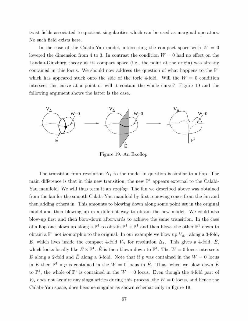
twist fields associated to quotient singularities which can be used as marginal operators.

No such field exists here.

In the case of the Calabi-Yau model, intersecting the compact space with W = 0

lowered the dimension from 4 to 3. In contrast the condition W = 0 had no effect on the

Landau-Ginzburg theory as its compact space (i.e., the point at the origin) was already

contained in this locus. We should now address the question of what happens to the P1

which has appeared stuck onto the side of the toric 4-fold. Will the W = 0 condition

intersect this curve at a point or will it contain the whole curve? Figure 19 and the

following argument shows the latter is the case.

W=0

Ε

W=0

P1

V∆ V∆

Ε

W=0V∆

Figure 19. An Exoflop.

The transition from resolution ∆1 to the model in question is similar to a flop. The

main difference is that in this new transition, the new P1 appears external to the Calabi-

Yau manifold. We will thus term it an exoflop. The fan we described above was obtained

from the fan for the smooth Calabi-Yau manifold by first removing cones from the fan and

then adding others in. This amounts to blowing down along some point set in the original

model and then blowing up in a different way to obtain the new model. We could also

blow-up first and then blow-down afterwards to achieve the same transition. In the case

of a flop one blows up along a P1 to obtain P1 × P1 and then blows the other P1 down to

obtain a P1 not isomorphic to the original. In our example we blow up V∆+ along a 3-fold,

E, which lives inside the compact 4-fold V∆ for resolution ∆1. This gives a 4-fold, E,

which looks locally like E × P1. E is then blown-down to P1. The W = 0 locus intersects

E along a 2-fold and E along a 3-fold. Note that if p was contained in the W = 0 locus

in E then P1 × p is contained in the W = 0 locus in E. Thus, when we blow down E

to P1, the whole of P1 is contained in the W = 0 locus. Even though the 4-fold part of

V∆ does not acquire any singularities during this process, the W = 0 locus, and hence the

Calabi-Yau space, does become singular as shown schematically in figure 19.

67

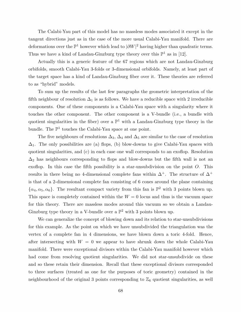
The Calabi-Yau part of this model has no massless modes associated it except in the

tangent directions just as in the case of the more usual Calabi-Yau manifold. There are

deformations over the P1 however which lead to |∂W |2 having higher than quadratic terms.

Thus we have a kind of Landau-Ginzburg type theory over this P1 as in [12].

Actually this is a generic feature of the 67 regions which are not Landau-Ginzburg

orbifolds, smooth Calabi-Yau 3-folds or 3-dimensional orbifolds. Namely, at least part of

the target space has a kind of Landau-Ginzburg fiber over it. These theories are referred

to as “hybrid” models.

To sum up the results of the last few paragraphs the geometric interpretation of the

fifth neighbour of resolution ∆1 is as follows. We have a reducible space with 2 irreducible

components. One of these components is a Calabi-Yau space with a singularity where it

touches the other component. The other component is a V-bundle (i.e., a bundle with

quotient singularities in the fiber) over a P1 with a Landau-Ginzburg type theory in the

bundle. The P1 touches the Calabi-Yau space at one point.

The five neighbours of resolutions ∆3, ∆4 and ∆5 are similar to the case of resolution

∆1. The only possibilities are (a) flops, (b) blow-downs to give Calabi-Yau spaces with

quotient singularities, and (c) in each case one wall corresponds to an exoflop. Resolution

∆2 has neighbours corresponding to flops and blow-downs but the fifth wall is not an

exoflop. In this case the fifth possibility is a star-unsubdivision on the point O. This

results in there being no 4-dimensional complete fans within ∆+. The structure of ∆+

is that of a 2-dimensional complete fan consisting of 6 cones around the plane containing

{α4, α5, α6}. The resultant compact variety from this fan is P2 with 3 points blown up.

This space is completely contained within the W = 0 locus and thus is the vacuum space

for this theory. There are massless modes around this vacuum so we obtain a Landau-

Ginzburg type theory in a V-bundle over a P2 with 3 points blown up.

We can generalize the concept of blowing down and its relation to star-unsubdivisions

for this example. As the point on which we have unsubdivided the triangulation was the

vertex of a complete fan in 4 dimensions, we have blown down a toric 4-fold. Hence,

after intersecting with W = 0 we appear to have shrunk down the whole Calabi-Yau

manifold. There were exceptional divisors within the Calabi-Yau manifold however which

had come from resolving quotient singularities. We did not star-unsubdivide on these

and so these retain their dimension. Recall that these exceptional divisors corresponded

to three surfaces (treated as one for the purposes of toric geometry) contained in the

neighbourhood of the original 3 points corresponding to Z6 quotient singularities, as well

68

as three divisors generally of the form P1×(curve) coming from the non-isolated Z2 and Z3

singularities. When we do the “blow-down” corresponding to the star-unsubdivision at α0

we set to zero all distances within the Calabi-Yau manifold that did not arise from resolving

singularities. Thus, the three surfaces become one since they are now zero distance apart

and the three divisors of the form P1×(curve) become P1’s. These P1’s are simply the 3

points blown up on the P2. This process is depicted in figure 20.

Figure 20. Blowing down the whole Calabi-Yau.

The above theory should be thought of as a natural step in the general process of

moving from a Calabi-Yau manifold to a Landau-Ginzburg theory. Whereas in the simpler

case studied in [12] there was a direct transition from a Calabi-Yau 3-fold immediately

down to a point giving a Landau-Ginzburg theory, our example appears to proceed more

naturally by steps. The original Calabi-Yau 3-fold moves down to a 2-fold and then one

can show there are models corresponding to 1-folds between this and the Landau-Ginzburg

point model.

The analysis of subsection 4.3 can now be repeated for the whole secondary fan. That

is, for each cone we take a “large radius limit” by following a line out to ∞ within a cone.

In the case of the 95 cones that do not give smooth Calabi-Yau manifolds this will not,

in fact, be a purely large radius limit but rather some kind of generalized geometric limit.

That is, it is the limit where the geometrical interpretation becomes exact. If this limit is

not taken then there are some kind of instanton (or anti-instanton) corrections in the sense

of [12]. If a generic value of the B-field is taken, then transitions from one cone to another

have no singularities. Thus, transitions between all the bizarre geometrical interpretations

we have described in this section are just as smooth as flop transitions in conformal field

theory.

69

7. Conclusions

A fascinating aspect of string theory is the interplay between operations and con-

structs on the world-sheet and their corresponding manifestations in spacetime. Familiar

examples include the relationship between world-sheet and spacetime supersymmetry and

the connection between world-sheet Kac-Moody symmetries and spacetime gauge symme-

tries. Part of the purpose of the present work has been to show another, rather striking,

correspondence. Namely, the world-sheet operation of deformation by a truly marginal

operator can, in certain circumstances, have a macroscopic interpretation as a change in

the topology of spacetime. We have thus shown the truth of the long held suspicion that in

string theory there are physical processes leading to a change in the topology of spacetime.

In fact, we have shown that these processes are in no way special or exotic — as they

correspond to changing the expectation value of a truly marginal operator, these processes

are amongst the most basic phenomena in conformal field theory.

More generally, the present work has set out to elucidate the structure of Calabi-Yau

moduli space from a more global perspective than has previously been undertaken. We

have seen that such a vantage point uncovers a wealth of rich and unexpected structure.

The geometrical interpretation of conformal field theory moduli space requires that we

augment the traditional Kahler moduli space associated with a Calabi-Yau space of a fixed

topological type to the enlarged Kahler moduli. The latter, as we have discussed, is a space

consisting of numerous regions adjoined along common walls. These regions consist of the

Kahler moduli spaces for: topologically distinct Calabi-Yau manifolds related by flops,

singular orbifolds of smooth Calabi-Yau manifolds, Landau-Ginzburg conformal models

and also the exotic “hybrid” conformal field theories we have encountered. Moreover, we

have shown that one can pass in a physically smooth manner between these regions. In

fact, under mirror symmetry, the whole enlarged Kahler moduli space corresponds to the

(ordinary) complex structure moduli space of the mirror Calabi-Yau space. Thus, passing

between regions in the Kahler moduli space generically corresponds to nothing more than

a smooth change in the complex structure of the mirror manifold.

In addition to learning that spacetime topology change can be realized in string theory,

the need to pass to the enlarged Kahler moduli space has resolved two important questions

in mirror symmetry and shed new light on the nature of orbifolds in string theory. For the

former we have seen that the work presented here resolves the apparent asymmetry between

complex and Kahler moduli spaces and also shows how the string deals with singularities

70

admitting distinct resolutions thereby clarifying the global picture of mirror symmetry.

For the latter we have seen that notion of orbifolds as boundary points in the walls of

the Kahler cone of the Calabi-Yau needs modification in the context of conformal field

theory/quantum algebraic geometry. Rather, orbifold theories occupy their own regions in

the enlarged Kahler moduli space and hence stand on equal footing with smooth Calabi-

Yau manifolds.

We confined most of our detailed discussion in section VI to those regions in the en-

larged Kahler moduli space corresponding to well studied theories such as Calabi-Yau and

orbifold backgrounds. It is interesting and important to gain an equally comprehensive

understanding of the regions corresponding to the less familiar hybrid theories. In fact,

if the example studied in section V is any indication, the majority of moduli space corre-

sponds to such theories! Their investigation is therefore of obvious merit and we intend to

report on such studies shortly.

Acknowledgements

We thank R. Plesser for important contributions at the inception and early stages of

this work. We gratefully acknowledge numerous invaluable discussions we have had with

E. Witten regarding both the present study and his closely related work [12]. We also

thank S. Katz, S.-S. Roan, and R. Wentworth for discussions. B.R.G. thanks S.-T. Yau for

suggesting the importance of studying flops in conformal field theory. The work of P.S.A.

was supported by DOE grant DE-FG02-90ER40542, the work of B.R.G. was supported by

the Ambrose Monell Foundation, by a National Young Investigator award and by the Alfred

P. Sloan foundation, and the work of D.R.M. was supported by NSF grant DMS-9103827

and by an American Mathematical Society Centennial Fellowship.

71

References

[1] L. Dixon, J. Harvey, C. Vafa and E. Witten, Nucl. Phys. B261 (1985) 678; Nucl.

Phys. B274 (1986) 285.

[2] L. Dixon, in Superstrings, Unified Theories and Cosmology 1987 (G. Furlan et al.,

eds.), World Scientific, 1988, p. 67.

[3] W. Lerche, C. Vafa and N. Warner, Nucl. Phys. B324 (1989) 427.

[4] P. Candelas, M. Lynker and R. Schimmrigk, Nucl. Phys. B341 (1990) 383.

[5] B.R. Greene and M.R. Plesser, Nucl. Phys. B338 (1990) 15.

[6] P. Candelas and X.C. De La Ossa, Nucl. Phys. B355 (1991) 455;

A.Strominger, Commun. Math. Phys. 133 (1990) 163;

S. Cecotti. S. Ferrara and L. Girardello, Phys. Lett. 213B (1989) 443.

[7] E. Viehweg, Invent. Math. 101 (1990) 521.

[8] P.S. Aspinwall, B.R. Greene and D.R. Morrison, Phys. Lett. 303B (1993) 249.

[9] G. Tian and S.-T. Yau, in Mathematical Aspects of String Theory (S.-T. Yau, ed.),

World Scientific, 1987, p. 543.

[10] J. Kollar, Nagoya Math. J. 113 (1989) 15.

[11] P. Candelas, P. Green and T. Hubsch, Nucl. Phys. B330 (1990) 49.

[12] E. Witten, Nucl. Phys. B403 (1993) 159.

[13] S.-S. Roan, Internat. J. Math. 2 (1991) 439; “Topological Properties of Calabi-Yau

Mirror Manifolds”, Max-Planck-Institut preprint, 1992.

[14] V. Batyrev, “Dual Polyhedra and Mirror Symmetry for Calabi-Yau Hypersurfaces in

Toric Varieties”, Essen preprint, November 18, 1992.

[15] D. Gepner, Phys. Lett. 199B (1987) 380.

[16] B. Greene, C. Vafa and N. Warner, Nucl. Phys. B324 (1989) 371.

[17] E. Martinec, in V.G. Knizhnik Memorial Volume (L. Brink et al., eds.), World Scien-

tific, 1990, p. 389; Phys. Lett. 217B (1989) 431.

[18] P.S. Aspinwall, Commun. Math. Phys. 128 (1990) 593.

[19] P.S. Aspinwall and C.A. Lutken, Nucl. Phys. B355 (1991) 482.

[20] S.-T. Yau, Proc. Nat. Acad. Sci. U.S.A. 74 (1977) 1798.

[21] F.A. Bogomolov, Dokl. Akad. Nauk SSSR 243 (1978), no. 5, 1101;

G. Tian, in Mathematical Aspects of String Theory (S.-T. Yau, ed.), World Scientific,

1987, p. 629;

A. Todorov, Commun. Math. Phys. 126 (1989) 325.

[22] P. Green and T. Hubsch, Commun. Math. Phys. 113 (1987) 505.

[23] P. Candelas and X.C. de la Ossa, Nucl. Phys. B342 (1990) 246.

[24] V. Guillemin and S. Sternberg, Invent. Math. 97 (1989) 485.

[25] R. Friedman, Proc. Symp. Pure Math. 53 (1991) 103.

[26] A. Strominger and E. Witten, Commun. Math. Phys. 101 (1985) 341.

72

[27] A. Strominger, Phys. Rev. Lett. 55 (1985) 2547.

[28] M. Dine, N. Seiberg, X.-G. Wen, and E. Witten, Nucl. Phys. B278 (1987) 769; Nucl.

Phys. B289 (1987) 319.

[29] P. Candelas, X.C. de la Ossa, P.S. Green, and L. Parkes, Phys. Lett. 258B (1991)

118; Nucl. Phys. B359 (1991) 21.

[30] P.S. Aspinwall and D.R. Morrison, Commun. Math. Phys. 151 (1993) 245.

[31] D.R. Morrison, J. Amer. Math. Soc. 6 (1993) 223.

[32] D.R. Morrison, in Essays on Mirror Manifolds (S.-T. Yau, ed.), International Press,

1992, p. 241;

A. Font, Nucl. Phys. B391 (1993) 358;

A. Klemm and S. Theisen, Nucl. Phys. B389 (1993) 153;

A. Libgober and J. Teitelbaum, Int. Math. Res. Notices (1993) 15;

V. Batyrev and D. van Straten, “Generalized Hypergeometric Functions and Rational

Curves on Calabi-Yau Complete Intersections in Toric Varieties”, Essen preprint, 1993;

P. Candelas, X. de la Ossa, A. Font, S. Katz and D.R. Morrison, “Mirror Symmetry

for Two Parameter Models – I”, CERN preprint CERN-TH.6884/93;

S. Hosono, A. Klemm, S. Theisen and S.-T. Yau, “Mirror Symmetry, Mirror Map and

Applications to Calabi-Yau Hypersurfaces”, Harvard preprint HUTMP-93/0801.

[33] P.S. Aspinwall, C.A. Lutken, and G.G. Ross, Phys. Lett. 241B (1990) 373.

[34] T. Oda, Convex Bodies and Algebraic Geometry, Springer-Verlag, 1988.

[35] W. Fulton, Introduction to Toric Varieties, Annals of Math. Studies, vol. 131, Prince-

ton University Press, 1993.

[36] M. Reid, in Journees de geometrie algebrique d’Angers (A. Beauville, ed.), Sijthoff &

Noordhoff, 1980, p. 273.

[37] P.S. Aspinwall, B.R. Greene and D.R. Morrison, “The Monomial-Divisor Mirror Map”,

IASSNS-HEP-93/43.

[38] S.-S. Roan, Internat. J. Math. 1 (1990) 211.

[39] D.A. Cox, “The Homogeneous Coordinate Ring of a Toric Variety”, Amherst preprint,

1992.

[40] M. Audin, The Topology of Torus Actions on Symplectic Manifolds, Progress in Math.,

vol. 93, Birkhauser, 1991.

[41] T. Oda and H.S. Park, Tohoku Math. J. 43 (1991) 375.

[42] L.J. Billera, P. Filliman, and B. Sturmfels, Adv. Math. 83 (1990) 155.

[43] E. Witten, Nucl. Phys. B268 (1985) 79; in Essays on Mirror Manifolds, (S.-T. Yau,

ed.), International Press Co., 1992, p. 120.

[44] J. Distler and B. Greene, Nucl. Phys. B309 (1988) 295.

[45] P.S. Aspinwall, B.R. Greene and D.R. Morrison, “Limit Points in the Moduli Space

of N=2 Conformal Sigma Models”, IASSNS-HEP-93/49, in preparation.

73

[46] D. Markushevich, M. Olshanetsky and A. Perelomov, Commun. Math. Phys. 111

(1987) 247.

[47] P. Candelas, Nucl. Phys. B298 (1988) 458.

[48] C. Vafa and N. Warner, Phys. Lett. 218B (1989) 51.

[49] V. Batyrev, Quantum cohomology rings of toric manifolds, MSRI preprint, 1993.

74