
c683-d chap 3a pp63-232:Rock...
81
3.3 Quarried rock – intrinsic properties CIRIA C683 97 1 3 4 10 9 8 7 6 5 2 (3.3) NOTE: The apparent mass density is to be used for design of hydraulic works. 3.3.3.3 Degree of saturation in stability calculations The value of mass density ρ app that is used when applying armourstone stability formulae, eg Hudson and Van der Meer (see Section 5.2.2.2), has traditionally been assumed to be the saturated surface dry mass density as it was considered the most applicable density term for armourstone in the intertidal zone under wave action. When fully saturated, the value of ρ app is therefore the value determined by testing in a saturated surface dry condition (ie degree of saturation, S r = 100 per cent). More recently, it has been recognised that different degrees of saturation are appropriate for stones in different zones of the structure. A correction to the density is now recommended for stability calculations to reflect the lower stability of blocks in the intertidal zone when they are not fully saturated. An assumed saturation of 25 per cent is recommended for armourstone that is not in permanent contact with water and for armourstone permanently below water, a saturation of 50 per cent is suggested (Laan, 1999); see also Table 3.17. Box 3.5 Effect of water saturation on apparent mass density For material with limited water absorption, the water content has a limited influence on the apparent density. However, for rock displaying a larger water absorption or porosity, the additional mass density attributable to the mass of water existing in the pores may be accounted for. Figure 3.9 gives the additional mass density due to the amount of water absorbed in accordance with Equation 3.3. Figure 3.9 Effect of degree of saturation S r (-), on the apparent mass density of porous rock ρ app . Contours indicate the correction value (in t/m³) to be added to the dry mass density ρ rock For example, a rock with dry mass density of 2.4 t/m³ and a porosity of 10 per cent (p = 0.1) has a correction value of 0.05 t/m³ for degree of saturation, S r = 50 per cent and 0.10 t/m³ for a fully saturated situation. In other words, the apparent mass density is 2.45 t/m³ or 2.50 t/m³ for 50 per cent or 100 per cent saturation respectively. ρ ρ ρ app rock w r = p p S ⋅ ⋅ ⋅ (1- ) +
Transcript of c683-d chap 3a pp63-232:Rock...
3.3 Quarried rock – intrinsic properties
CIRIA C683 97
1
3
4
10
9
8
7
6
5
2
(3.3)
NOTE: The apparent mass density is to be used for design of hydraulic works.
3.3.3.3 Degree of saturation in stability calculations
The value of mass density ρapp that is used when applying armourstone stability formulae, egHudson and Van der Meer (see Section 5.2.2.2), has traditionally been assumed to be thesaturated surface dry mass density as it was considered the most applicable density term forarmourstone in the intertidal zone under wave action. When fully saturated, the value of ρappis therefore the value determined by testing in a saturated surface dry condition (ie degree ofsaturation, Sr = 100 per cent). More recently, it has been recognised that different degrees ofsaturation are appropriate for stones in different zones of the structure. A correction to thedensity is now recommended for stability calculations to reflect the lower stability of blocks inthe intertidal zone when they are not fully saturated. An assumed saturation of 25 per cent isrecommended for armourstone that is not in permanent contact with water and forarmourstone permanently below water, a saturation of 50 per cent is suggested (Laan, 1999);see also Table 3.17.
Box 3.5 Effect of water saturation on apparent mass density
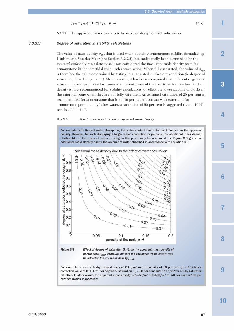
For material with limited water absorption, the water content has a limited influence on the apparentdensity. However, for rock displaying a larger water absorption or porosity, the additional mass densityattributable to the mass of water existing in the pores may be accounted for. Figure 3.9 gives theadditional mass density due to the amount of water absorbed in accordance with Equation 3.3.
Figure 3.9 Effect of degree of saturation Sr (-), on the apparent mass density of porous rock ρapp. Contours indicate the correction value (in t/m³) to be added to the dry mass density ρrock
For example, a rock with dry mass density of 2.4 t/m³ and a porosity of 10 per cent (p = 0.1) has acorrection value of 0.05 t/m³ for degree of saturation, Sr = 50 per cent and 0.10 t/m³ for a fully saturatedsituation. In other words, the apparent mass density is 2.45 t/m³ or 2.50 t/m³ for 50 per cent or 100 percent saturation respectively.
ρ ρ ρapp rock w r= p p S⋅ ⋅ ⋅(1- ) +
3.3 Quarried rock – intrinsic properties
CIRIA C683 99
1
3
4
10
9
8
7
6
5
2
Major breakage refers to breakage of individual armour stones along pre-existing defects, asshown in Figure 3.10 for armourstone with different geological origins. Any defects arecontrolled by the geology of the rock source and the production technique. For example,sedimentary rocks may contain bedding planes, stylolites, calcite veins or shaly partings, whileigneous rocks may contain mineral veins, contacts between distinct petrographic units orcooling cracks. In addition, macro-flaws may be induced by blasting or fragmentation of therock mass during extraction. If these defects propagate, a proportion of stones will betransformed into large fragments. If major breakage takes place on a significant number ofstones, this may significantly affect the mass distribution of the armourstone andconsequently the value of design parameters such as M50 or Dn50 (see Section 3.6.6).Resistance to major breakage is known as integrity.
Minor breakage refers to breakages of asperities. This often occurs when stone edges orcorners are knocked off during routine handling, by the traffic of heavy plant duringconstruction, or during initial settlement of the structure (see Figure 3.11). Thisphenomenon takes place along new fractures created through the mineral fabric of the stone.It is often associated with bruising and crushing, and generally creates fragments of limitedsize (up to a few tens of kilogrammes) depending on the armourstone grading. Thisphenomenon has a limited impact on the mass distribution and the M50 value (see Section3.6.6), but can contribute to edge rounding. Many strength tests exist for measuring theresistance of mineral fabric to breakage and are discussed in Section 3.8.5 but they do notcorrelate with armourstone integrity tests (Perrier et al, 2004).
In simple terms, armourstone integrity is the ability of armourstone pieces to withstandexcessive breakage during their life cycle. It should not be confused with resistance tobreakage through the mineral fabric, ie resistance to minor breakage that might be tested onsmall laboratory specimens or aggregates. From a survey of feedback from 200 professionals,including designers, contractors, quarry companies, port and waterways authorities,armourstone integrity was identified as an essential property (Dupray, 2002). Two aspects ofintegrity should be distinguished.
1 The integrity of armourstone as an individual piece is its ability not to display excessivebreakage. The threshold for excessive breakage is discussed in Section 3.8.5.
2 The integrity of armourstone as a granular material is the ability of a consignment not todisplay excessive changes of mass distribution and especially of its characteristic masses.
Integrity is a property of heavy and light armourstone, among others such as shapecharacteristics, that may be evaluated by initial type tests, ie one-off tests giving informationabout an armourstone source to promote design optimisation. Such initial type testing isdistinct from routine testing of the quality of consignments in association with factoryproduction control.
3 Materials
CIRIA C683104
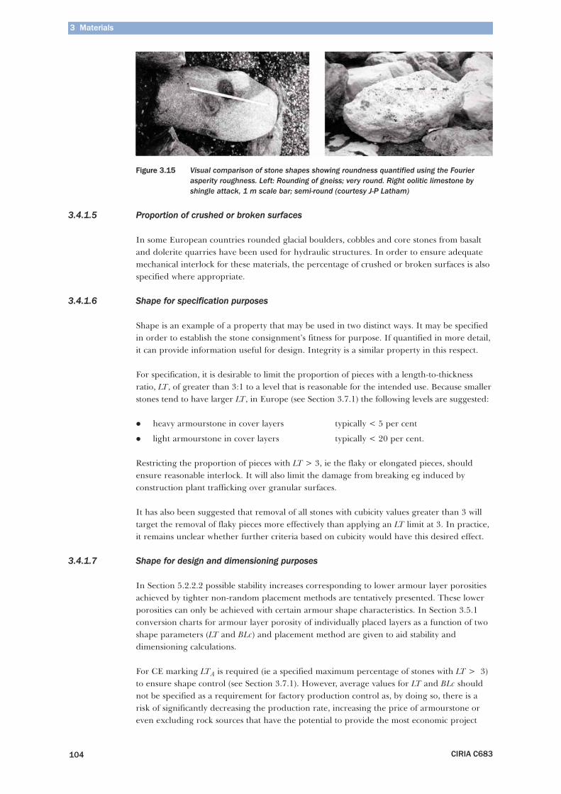
Figure 3.15 Visual comparison of stone shapes showing roundness quantified using the Fourierasperity roughness. Left: Rounding of gneiss; very round. Right oolitic limestone byshingle attack, 1 m scale bar; semi-round (courtesy J-P Latham)
3.4.1.5 Proportion of crushed or broken surfaces
In some European countries rounded glacial boulders, cobbles and core stones from basaltand dolerite quarries have been used for hydraulic structures. In order to ensure adequatemechanical interlock for these materials, the percentage of crushed or broken surfaces is alsospecified where appropriate.
3.4.1.6 Shape for specification purposes
Shape is an example of a property that may be used in two distinct ways. It may be specifiedin order to establish the stone consignment’s fitness for purpose. If quantified in more detail,it can provide information useful for design. Integrity is a similar property in this respect.
For specification, it is desirable to limit the proportion of pieces with a length-to-thicknessratio, LT, of greater than 3:1 to a level that is reasonable for the intended use. Because smallerstones tend to have larger LT, in Europe (see Section 3.7.1) the following levels are suggested:
� heavy armourstone in cover layers typically < 5 per cent
� light armourstone in cover layers typically < 20 per cent.
Restricting the proportion of pieces with LT > 3, ie the flaky or elongated pieces, shouldensure reasonable interlock. It will also limit the damage from breaking eg induced byconstruction plant trafficking over granular surfaces.
It has also been suggested that removal of all stones with cubicity values greater than 3 willtarget the removal of flaky pieces more effectively than applying an LT limit at 3. In practice,it remains unclear whether further criteria based on cubicity would have this desired effect.
3.4.1.7 Shape for design and dimensioning purposes
In Section 5.2.2.2 possible stability increases corresponding to lower armour layer porositiesachieved by tighter non-random placement methods are tentatively presented. These lowerporosities can only be achieved with certain armour shape characteristics. In Section 3.5.1conversion charts for armour layer porosity of individually placed layers as a function of twoshape parameters (LT and BLc) and placement method are given to aid stability anddimensioning calculations.
For CE marking LTA is required (ie a specified maximum percentage of stones with LT > 3)to ensure shape control (see Section 3.7.1). However, average values for LT and BLc shouldnot be specified as a requirement for factory production control as, by doing so, there is arisk of significantly decreasing the production rate, increasing the price of armourstone oreven excluding rock sources that have the potential to provide the most economic project
3 Materials
CIRIA C683110
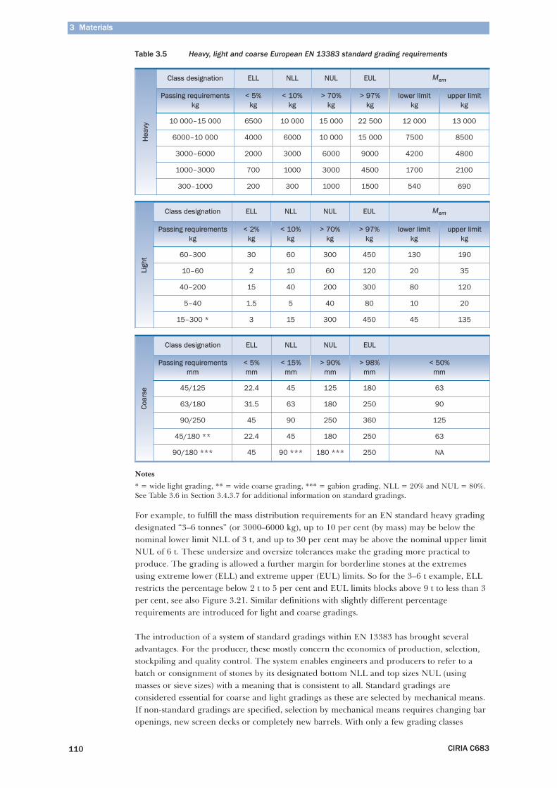
Table 3.5 Heavy, light and coarse European EN 13383 standard grading requirements
Notes
* = wide light grading, ** = wide coarse grading, *** = gabion grading, NLL = 20% and NUL = 80%.See Table 3.6 in Section 3.4.3.7 for additional information on standard gradings.
For example, to fulfill the mass distribution requirements for an EN standard heavy gradingdesignated “3–6 tonnes” (or 3000–6000 kg), up to 10 per cent (by mass) may be below thenominal lower limit NLL of 3 t, and up to 30 per cent may be above the nominal upper limitNUL of 6 t. These undersize and oversize tolerances make the grading more practical toproduce. The grading is allowed a further margin for borderline stones at the extremesusing extreme lower (ELL) and extreme upper (EUL) limits. So for the 3–6 t example, ELLrestricts the percentage below 2 t to 5 per cent and EUL limits blocks above 9 t to less than 3per cent, see also Figure 3.21. Similar definitions with slightly different percentagerequirements are introduced for light and coarse gradings.
The introduction of a system of standard gradings within EN 13383 has brought severaladvantages. For the producer, these mostly concern the economics of production, selection,stockpiling and quality control. The system enables engineers and producers to refer to abatch or consignment of stones by its designated bottom NLL and top sizes NUL (usingmasses or sieve sizes) with a meaning that is consistent to all. Standard gradings areconsidered essential for coarse and light gradings as these are selected by mechanical means.If non-standard gradings are specified, selection by mechanical means requires changing baropenings, new screen decks or completely new barrels. With only a few grading classes
Hea
vy
Class designation ELL NLL NUL EUL Mem
Passing requirementskg
< 5%kg
< 10%kg
> 70%kg
> 97%kg
lower limitkg
upper limitkg
10 000–15 000 6500 10 000 15 000 22 500 12 000 13 000
6000–10 000 4000 6000 10 000 15 000 7500 8500
3000–6000 2000 3000 6000 9000 4200 4800
1000–3000 700 1000 3000 4500 1700 2100
300–1000 200 300 1000 1500 540 690
Ligh
t
Class designation ELL NLL NUL EUL Mem
Passing requirementskg
< 2%kg
< 10%kg
> 70%kg
> 97%kg
lower limitkg
upper limitkg
60–300 30 60 300 450 130 190
10–60 2 10 60 120 20 35
40–200 15 40 200 300 80 120
5–40 1.5 5 40 80 10 20
15–300 * 3 15 300 450 45 135
Coar
se
Class designation ELL NLL NUL EUL
Passing requirementsmm
< 5%mm
< 15%mm
> 90%mm
> 98%mm
< 50%mm
45/125 22.4 45 125 180 63
63/180 31.5 63 180 250 90
90/250 45 90 250 360 125
45/180 ** 22.4 45 180 250 63
90/180 *** 45 90 *** 180 *** 250 NA
3.4 Quarried rock – production-induced properties
CIRIA C683 113
1
3
4
10
9
8
7
6
5
2
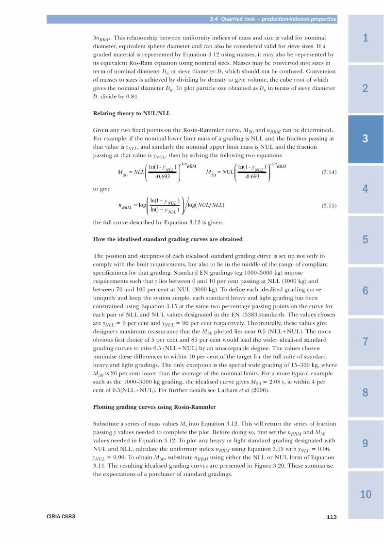
3nRRM. This relationship between uniformity indices of mass and size is valid for nominaldiameter, equivalent sphere diameter and can also be considered valid for sieve sizes. If agraded material is represented by Equation 3.12 using masses, it may also be represented byits equivalent Ros-Ram equation using nominal sizes. Masses may be converted into sizes interm of nominal diameter Dn or sieve diameter D, which should not be confused. Conversionof masses to sizes is achieved by dividing by density to give volume, the cube root of whichgives the nominal diameter Dn. To plot particle size obtained as Dn in terms of sieve diameterD, divide by 0.84.
Relating theory to NUL/NLL
Given any two fixed points on the Rosin-Rammler curve, M50 and nRRM can be determined.For example, if the nominal lower limit mass of a grading is NLL and the fraction passing atthat value is yNLL, and similarly the nominal upper limit mass is NUL and the fractionpassing at that value is yNUL, then by solving the following two equations:
(3.14)
to give
(3.15)
the full curve described by Equation 3.12 is given.
How the idealised standard grading curves are obtained
The position and steepness of each idealised standard grading curve is set up not only tocomply with the limit requirements, but also to lie in the middle of the range of compliantspecifications for that grading. Standard EN gradings (eg 1000–3000 kg) imposerequirements such that y lies between 0 and 10 per cent passing at NLL (1000 kg) andbetween 70 and 100 per cent at NUL (3000 kg). To define each idealised grading curveuniquely and keep the system simple, each standard heavy and light grading has beenconstrained using Equation 3.15 at the same two percentage passing points on the curve foreach pair of NLL and NUL values designated in the EN 13383 standards. The values chosenare yNLL = 6 per cent and yNUL = 90 per cent respectively. Theoretically, these values givedesigners maximum reassurance that the M50 plotted lies near 0.5 (NLL+NUL). The moreobvious first choice of 5 per cent and 85 per cent would lead the wider idealised standardgrading curves to miss 0.5 (NLL+NUL) by an unacceptable degree. The values chosenminimise these differences to within 10 per cent of the target for the full suite of standardheavy and light gradings. The only exception is the special wide grading of 15–300 kg, whereM50 is 26 per cent lower than the average of the nominal limits. For a more typical examplesuch as the 1000–3000 kg grading, the idealised curve gives M50 = 2.08 t, ie within 4 percent of 0.5(NLL+NUL). For further details see Latham et al (2006).
Plotting grading curves using Rosin-Rammler
Substitute a series of mass values My into Equation 3.12. This will return the series of fractionpassing y values needed to complete the plot. Before doing so, first set the nRRM and M50values needed in Equation 3.12. To plot any heavy or light standard grading designated withNUL and NLL, calculate the uniformity index nRRM using Equation 3.15 with yNLL = 0.06,yNUL = 0.90. To obtain M50, substitute nRRM using either the NLL or NUL form of Equation3.14. The resulting idealised grading curves are presented in Figure 3.20. These summarisethe expectations of a purchaser of standard gradings.
M NLLy
M NULNLLnRRM
50
-1/
50 =
1n(1- )
-0.693 =
1⎛
⎝⎜⎜
⎞
⎠⎟⎟
nn(1- )
-0.693
-1/yNULnRRM ⎛
⎝⎜⎜
⎞
⎠⎟⎟
nyy
NUL NLLRRMNUL
NLL=
−−
⎛
⎝⎜⎜
⎞
⎠⎟⎟log
ln( )
ln( )log( )
1
1
3.4 Quarried rock – production-induced properties
CIRIA C683 119
1
3
4
10
9
8
7
6
5
2
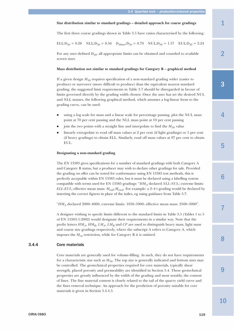
Size distribution similar to standard gradings – detailed approach for coarse gradings
The first three coarse gradings shown in Table 3.5 have ratios characterised by the following:
ELL/D50 = 0.28 NLL/D50 = 0.56 D50min/D50 = 0.79 NUL/D50 = 1.57 EUL/D50 = 2.24
For any user-defined D50, all appropriate limits can be obtained and rounded to availablescreen sizes.
Mass distribution not similar to standard gradings for Category B – graphical method
If a given design M50 requires specification of a non-standard grading wider (easier toproduce) or narrower (more difficult to produce) than the equivalent nearest standardgrading, the suggested limit requirements in Table 3.7 should be disregarded in favour oflimits governed directly by the grading width chosen. Once the user has set the desired NULand NLL masses, the following graphical method, which assumes a log-linear form to thegrading curve, can be used:
� using a log scale for mass and a linear scale for percentage passing, plot the NUL masspoint at 70 per cent passing and the NLL mass point at 10 per cent passing
� join the two points with a straight line and interpolate to find the M50 value
� linearly extrapolate to read off mass values at 2 per cent (if light gradings) or 5 per cent(if heavy gradings) to obtain ELL. Similarly, read off mass values at 97 per cent to obtainEUL.
Designating a non-standard grading
The EN 13383 gives specifications for a number of standard gradings with both Category Aand Category B status, but a producer may wish to declare other gradings for sale. Providedthe grading on offer can be tested for conformance using EN 13383 test methods, this isperfectly acceptable within EN 13383 rules, but it must be declared using a labelling systemcompatible with terms used for EN 13383 gradings: “HMA declared NLL-NUL; extreme limits:ELL-EUL; effective mean mass: Memll-Memul. For example: a 2–4 t grading would be declared byinserting the correct figures in place of the italics, eg using guidance from Table 3.7:
“HMA declared 2000–4000; extreme limits: 1050–5900; effective mean mass: 2500–3000”.
A designer wishing to specify limits different to the standard limits in Table 3.5 (Tables 1 to 5of EN 13383-1:2002) would designate their requirements in a similar way. Note that theprefix letters HMA, HMB, LMA, LMB and CP are used to distinguish heavy mass, light massand coarse size gradings respectively, where the subscript A refers to Category A, whichimposes the Mem restriction, while for Category B it is omitted.
3.4.4 Core materials
Core materials are generally used for volume-filling. As such, they do not have requirementsfor a characteristic size such as M50. The top size is generally indicated and bottom sizes maybe controlled. The geotechnical properties required for core materials, typically shearstrength, placed porosity and permeability are identified in Section 5.4. These geotechnicalproperties are greatly influenced by the width of the grading and most notably, the contentof fines. The fine material content is closely related to the tail of the quarry yield curve andthe fines removal technique. An approach for the prediction of porosity suitable for corematerials is given in Section 3.4.4.3.
3 Materials
CIRIA C683124
properties, the type of placements assigned to granular materials in the works, are classified as:
� random placement
� standard placement
� dense placement
� specific placement.
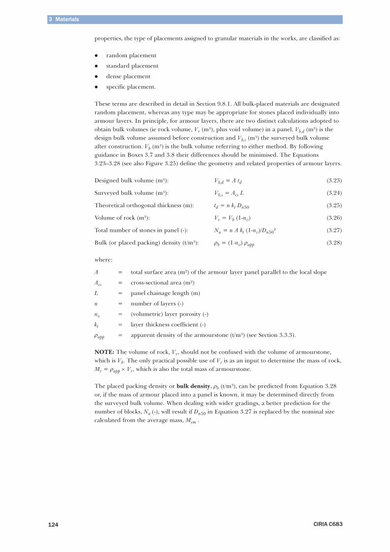
These terms are described in detail in Section 9.8.1. All bulk-placed materials are designatedrandom placement, whereas any type may be appropriate for stones placed individually intoarmour layers. In principle, for armour layers, there are two distinct calculations adopted toobtain bulk volumes (ie rock volume, Vr (m³), plus void volume) in a panel. Vb,d (m³) is thedesign bulk volume assumed before construction and Vb,s (m³) the surveyed bulk volumeafter construction. Vb (m³) is the bulk volume referring to either method. By followingguidance in Boxes 3.7 and 3.8 their differences should be minimised. The Equations3.23–3.28 (see also Figure 3.25) define the geometry and related properties of armour layers.
Designed bulk volume (m³): Vb,d = A td (3.23)
Surveyed bulk volume (m³): Vb,s = Acs L (3.24)
Theoretical orthogonal thickness (m): td = n kt Dn50 (3.25)
Volume of rock (m³): Vr = Vb (1-nv) (3.26)
Total number of stones in panel (-): Na = n A kt (1-nv)/Dn50² (3.27)
Bulk (or placed packing) density (t/m³): ρb = (1-nv) ρapp (3.28)
where:
A = total surface area (m²) of the armour layer panel parallel to the local slope
Acs = cross-sectional area (m²)
L = panel chainage length (m)
n = number of layers (-)
nv = (volumetric) layer porosity (-)
kt = layer thickness coefficient (-)
ρapp = apparent density of the armourstone (t/m³) (see Section 3.3.3).
NOTE: The volume of rock, Vr, should not be confused with the volume of armourstone,which is Vb. The only practical possible use of Vr is as an input to determine the mass of rock,Mr = ρapp × Vr, which is also the total mass of armourstone.
The placed packing density or bulk density, ρb (t/m³), can be predicted from Equation 3.28or, if the mass of armour placed into a panel is known, it may be determined directly fromthe surveyed bulk volume. When dealing with wider gradings, a better prediction for thenumber of blocks, Na (-), will result if Dn50 in Equation 3.27 is replaced by the nominal sizecalculated from the average mass, Mem .
3 Materials
CIRIA C683138
3 Materials
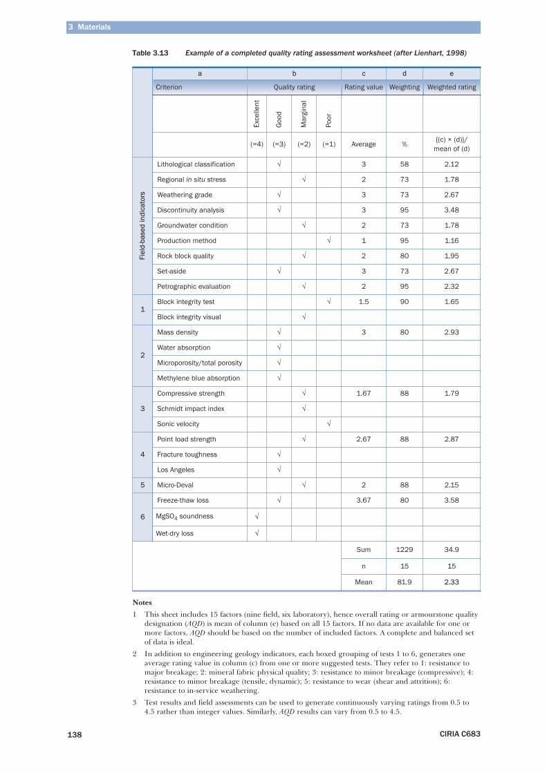
Table 3.13 Example of a completed quality rating assessment worksheet (after Lienhart, 1998)
Notes
1 This sheet includes 15 factors (nine field, six laboratory), hence overall rating or armourstone qualitydesignation (AQD) is mean of column (e) based on all 15 factors. If no data are available for one ormore factors, AQD should be based on the number of included factors. A complete and balanced setof data is ideal.
2 In addition to engineering geology indicators, each boxed grouping of tests 1 to 6, generates oneaverage rating value in column (c) from one or more suggested tests. They refer to 1: resistance tomajor breakage; 2: mineral fabric physical quality; 3: resistance to minor breakage (compressive); 4:resistance to minor breakage (tensile, dynamic); 5: resistance to wear (shear and attrition); 6:resistance to in-service weathering.
3 Test results and field assessments can be used to generate continuously varying ratings from 0.5 to4.5 rather than integer values. Similarly, AQD results can vary from 0.5 to 4.5.
a b c d e
Criterion Quality rating Rating value Weighting Weighted rating
Exce
llent
Goo
d
Mar
gina
l
Poor
(=4) (=3) (=2) (=1) Average %{(c) × (d)}/
mean of (d) Fi
eld-
base
d in
dica
tors
Lithological classification √ 3 58 2.12
Regional in situ stress √ 2 73 1.78
Weathering grade √ 3 73 2.67
Discontinuity analysis √ 3 95 3.48
Groundwater condition √ 2 73 1.78
Production method √ 1 95 1.16
Rock block quality √ 2 80 1.95
Set-aside √ 3 73 2.67
Petrographic evaluation √ 2 95 2.32
1Block integrity test √ 1.5 90 1.65
Block integrity visual √
2
Mass density √ 3 80 2.93
Water absorption √
Microporosity/total porosity √
Methylene blue absorption √
3
Compressive strength √ 1.67 88 1.79
Schmidt impact index √
Sonic velocity √
4
Point load strength √ 2.67 88 2.87
Fracture toughness √
Los Angeles √
5 Micro-Deval √ 2 88 2.15
6
Freeze-thaw loss √ 3.67 80 3.58
MgSO4 soundness √
Wet-dry loss √
Sum 1229 34.9
n 15 15
Mean 81.9 2.33
3.6 Rock quality, durability and service-life prediction
CIRIA C683 139
1
3
4
10
9
8
7
6
5
2
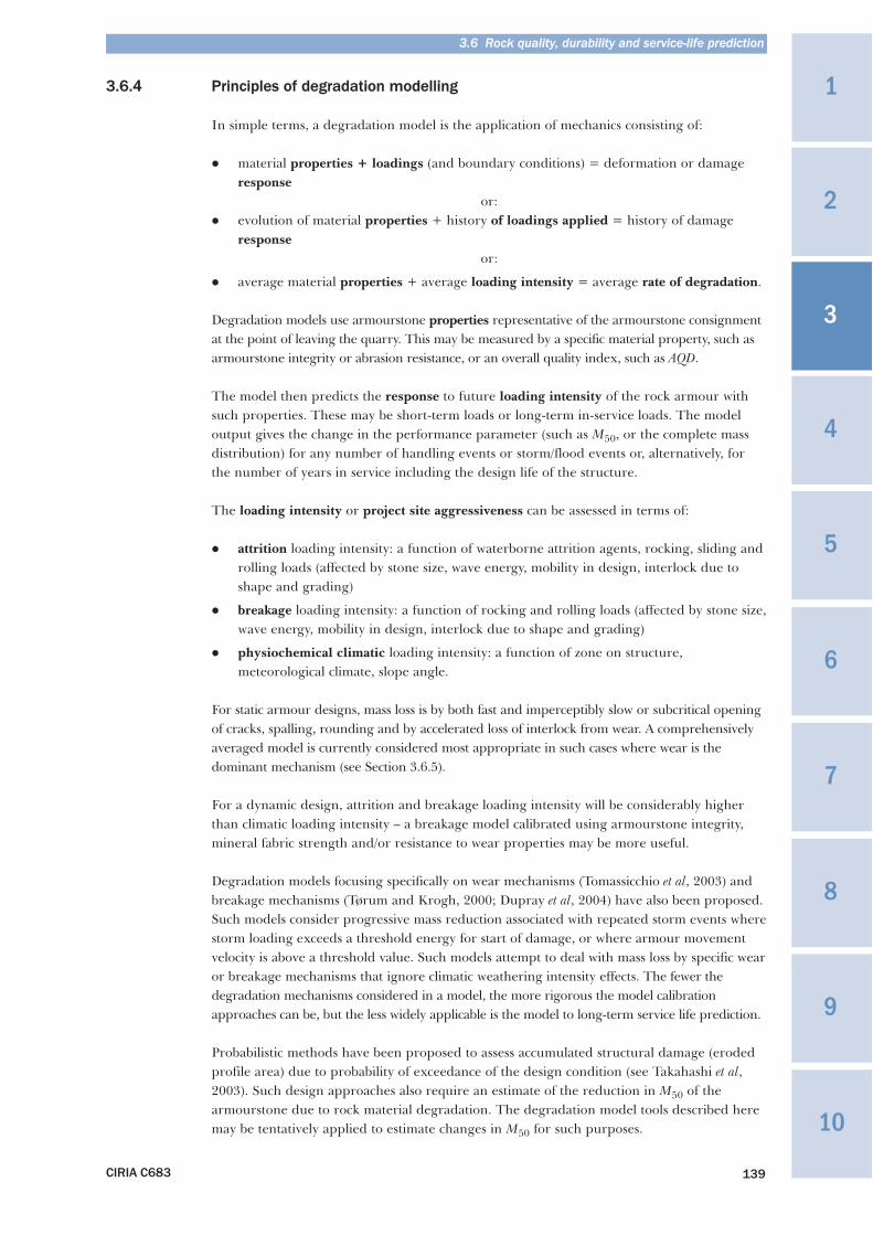
3.6.4 Principles of degradation modelling
In simple terms, a degradation model is the application of mechanics consisting of:
� material properties + loadings (and boundary conditions) = deformation or damageresponse
or:� evolution of material properties + history of loadings applied = history of damage
responseor:
� average material properties + average loading intensity = average rate of degradation.
Degradation models use armourstone properties representative of the armourstone consignmentat the point of leaving the quarry. This may be measured by a specific material property, such asarmourstone integrity or abrasion resistance, or an overall quality index, such as AQD.
The model then predicts the response to future loading intensity of the rock armour withsuch properties. These may be short-term loads or long-term in-service loads. The modeloutput gives the change in the performance parameter (such as M50, or the complete massdistribution) for any number of handling events or storm/flood events or, alternatively, forthe number of years in service including the design life of the structure.
The loading intensity or project site aggressiveness can be assessed in terms of:
� attrition loading intensity: a function of waterborne attrition agents, rocking, sliding androlling loads (affected by stone size, wave energy, mobility in design, interlock due toshape and grading)
� breakage loading intensity: a function of rocking and rolling loads (affected by stone size,wave energy, mobility in design, interlock due to shape and grading)
� physiochemical climatic loading intensity: a function of zone on structure,meteorological climate, slope angle.
For static armour designs, mass loss is by both fast and imperceptibly slow or subcritical openingof cracks, spalling, rounding and by accelerated loss of interlock from wear. A comprehensivelyaveraged model is currently considered most appropriate in such cases where wear is thedominant mechanism (see Section 3.6.5).
For a dynamic design, attrition and breakage loading intensity will be considerably higherthan climatic loading intensity – a breakage model calibrated using armourstone integrity,mineral fabric strength and/or resistance to wear properties may be more useful.
Degradation models focusing specifically on wear mechanisms (Tomassicchio et al, 2003) andbreakage mechanisms (Tørum and Krogh, 2000; Dupray et al, 2004) have also been proposed.Such models consider progressive mass reduction associated with repeated storm events wherestorm loading exceeds a threshold energy for start of damage, or where armour movementvelocity is above a threshold value. Such models attempt to deal with mass loss by specific wearor breakage mechanisms that ignore climatic weathering intensity effects. The fewer thedegradation mechanisms considered in a model, the more rigorous the model calibrationapproaches can be, but the less widely applicable is the model to long-term service life prediction.
Probabilistic methods have been proposed to assess accumulated structural damage (erodedprofile area) due to probability of exceedance of the design condition (see Takahashi et al,2003). Such design approaches also require an estimate of the reduction in M50 of thearmourstone due to rock material degradation. The degradation model tools described heremay be tentatively applied to estimate changes in M50 for such purposes.
3 Materials
CIRIA C683144
3 Materials
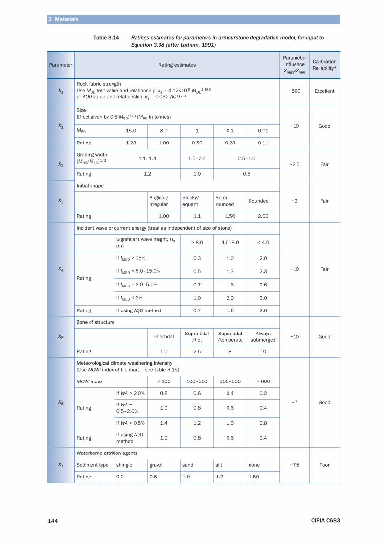
Table 3.14 Ratings estimates for parameters in armourstone degradation model, for input toEquation 3.38 (after Latham, 1991)
Parameter Rating estimatesParameterinfluenceXmax/Xmin
CalibrationReliability*
ks
Rock fabric strengthUse MDE test value and relationship: ks = 4.12×10⁻⁵ MDE
1.485
or AQD value and relationship: ks = 0.032 AQD-2.0~500 Excellent
X1
SizeEffect given by 0.5(M50)1/3 (M50 in tonnes)
~10 GoodM50 15.0 8.0 1 0.1 0.01
Rating 1.23 1.00 0.50 0.23 0.11
X2
Grading width(M85/M15)1/3 1.1–1.4 1.5–2.4 2.5–4.0
~2.5 Fair
Rating 1.2 1.0 0.5
X3
Initial shape
~2 FairAngular/irregular
Blocky/equant
Semi-rounded
Rounded
Rating 1.00 1.1 1.50 2.00
X4
Incident wave or current energy (treat as independent of size of stone)
~10 Fair
Significant wave height, Hs(m)
> 8.0 4.0–8.0 < 4.0
Rating
If IM50 > 15% 0.3 1.0 2.0
If IM50 = 5.0–15.0% 0.5 1.3 2.3
If IM50 = 2.0–5.0% 0.7 1.6 2.6
If IM50 < 2% 1.0 2.0 3.0
Rating If using AQD method 0.7 1.6 2.6
X5
Zone of structure
~10 GoodIntertidalSupra-tidal
/hotSupra-tidal/temperate
Alwayssubmerged
Rating 1.0 2.5 8 10
X6
Meteorological climate weathering intensity(Use MCWI index of Lienhart – see Table 3.15)
~7 Good
MCWI index < 100 100–300 300–600 > 600
Rating
If WA > 2.0% 0.8 0.6 0.4 0.2
If WA =0.5–2.0%
1.0 0.8 0.6 0.4
If WA < 0.5% 1.4 1.2 1.0 0.8
RatingIf using AQDmethod
1.0 0.8 0.6 0.4
X7
Waterborne attrition agents
~7.5 PoorSediment type shingle gravel sand silt none
Rating 0.2 0.5 1.0 1.2 1.50
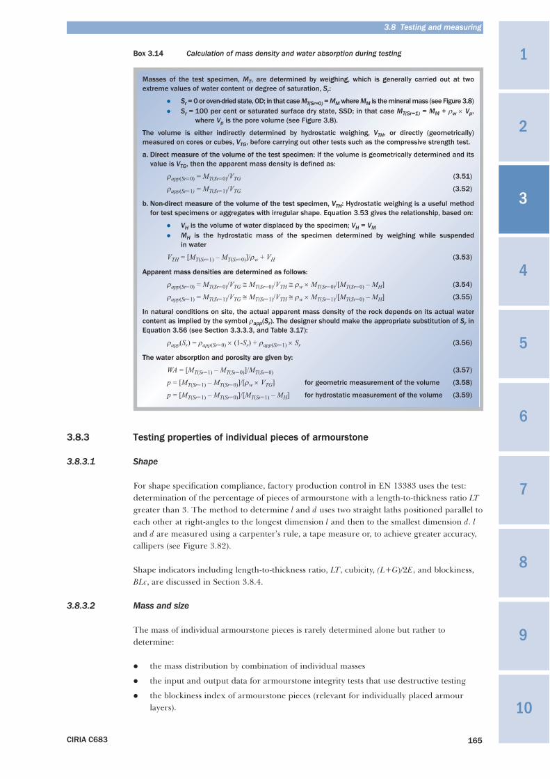
Box 3.14 Calculation of mass density and water absorption during testing
3.8.3 Testing properties of individual pieces of armourstone
3.8.3.1 Shape
For shape specification compliance, factory production control in EN 13383 uses the test:determination of the percentage of pieces of armourstone with a length-to-thickness ratio LTgreater than 3. The method to determine l and d uses two straight laths positioned parallel toeach other at right-angles to the longest dimension l and then to the smallest dimension d. land d are measured using a carpenter’s rule, a tape measure or, to achieve greater accuracy,callipers (see Figure 3.82).
Shape indicators including length-to-thickness ratio, LT, cubicity, (L+G)/2E, and blockiness,BLc, are discussed in Section 3.8.4.
3.8.3.2 Mass and size
The mass of individual armourstone pieces is rarely determined alone but rather todetermine:
� the mass distribution by combination of individual masses
� the input and output data for armourstone integrity tests that use destructive testing
� the blockiness index of armourstone pieces (relevant for individually placed armourlayers).
Xxxx
CIRIA C683 165
1
3
4
10
9
8
7
6
5
2
3.8 Testing and measuring
Masses of the test specimen, MT, are determined by weighing, which is generally carried out at twoextreme values of water content or degree of saturation, Sr:
� Sr = 0 or oven-dried state, OD; in that case MT(Sr=0) = MM where MM is the mineral mass (see Figure 3.8)� Sr = 100 per cent or saturated surface dry state, SSD; in that case MT(Sr=1) = MM + ρw × Vp,
where Vp is the pore volume (see Figure 3.8).
The volume is either indirectly determined by hydrostatic weighing, VTH, or directly (geometrically)measured on cores or cubes, VTG, before carrying out other tests such as the compressive strength test.
a. Direct measure of the volume of the test specimen: If the volume is geometrically determined and itsvalue is VTG, then the apparent mass density is defined as:
ρapp(Sr=0) = MT(Sr=0)/VTG (3.51)
ρapp(Sr=1) = MT(Sr=1)/VTG (3.52)
b. Non-direct measure of the volume of the test specimen, VTH: Hydrostatic weighing is a useful methodfor test specimens or aggregates with irregular shape. Equation 3.53 gives the relationship, based on:
� VH is the volume of water displaced by the specimen; VH = VM� MH is the hydrostatic mass of the specimen determined by weighing while suspended
in water
VTH = [MT(Sr=1) – MT(Sr=0)]/ρw + VH (3.53)
Apparent mass densities are determined as follows:
ρapp(Sr=0) = MT(Sr=0)/VTG ≅ MT(Sr=0)/VTH ≅ ρw × MT(Sr=0)/[MT(Sr=0) – MH] (3.54)
ρapp(Sr=1) = MT(Sr=1)/VTG ≅ MT(Sr=1)/VTH ≅ ρw × MT(Sr=1)/[MT(Sr=0) – MH] (3.55)
In natural conditions on site, the actual apparent mass density of the rock depends on its actual watercontent as implied by the symbol ρapp(Sr). The designer should make the appropriate substitution of Sr inEquation 3.56 (see Section 3.3.3.3, and Table 3.17):
ρapp(Sr) = ρapp(Sr=0) × (1-Sr) + ρapp(Sr=1) × Sr (3.56)
The water absorption and porosity are given by:
WA = [MT(Sr=1) – MT(Sr=0)]/MT(Sr=0) (3.57)
p = [MT(Sr=1) – MT(Sr=0)]/[ρw × VTG] for geometric measurement of the volume (3.58)
p = [MT(Sr=1) – MT(Sr=0)]/[MT(Sr=1) – MH] for hydrostatic measurement of the volume (3.59)
Xxxx
CIRIA C683 193
1
3
4
10
9
8
7
6
5
2
3.9 Quarry operations
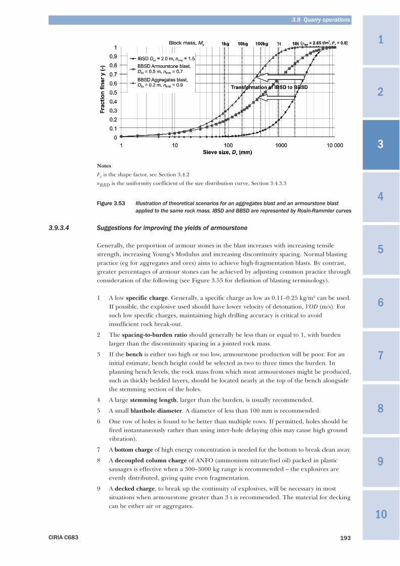
Notes
Fs is the shape factor, see Section 3.4.2
nRRD is the uniformity coefficient of the size distribution curve, Section 3.4.3.3
Figure 3.53 Illustration of theoretical scenarios for an aggregates blast and an armourstone blastapplied to the same rock mass. IBSD and BBSD are represented by Rosin-Rammler curves
3.9.3.4 Suggestions for improving the yields of armourstone
Generally, the proportion of armour stones in the blast increases with increasing tensilestrength, increasing Young’s Modulus and increasing discontinuity spacing. Normal blastingpractice (eg for aggregates and ores) aims to achieve high-fragmentation blasts. By contrast,greater percentages of armour stones can be achieved by adjusting common practice throughconsideration of the following (see Figure 3.55 for definition of blasting terminology).
1 A low specific charge. Generally, a specific charge as low as 0.11–0.25 kg/m³ can be used.If possible, the explosive used should have lower velocity of detonation, VOD (m/s). Forsuch low specific charges, maintaining high drilling accuracy is critical to avoidinsufficient rock break-out.
2 The spacing-to-burden ratio should generally be less than or equal to 1, with burdenlarger than the discontinuity spacing in a jointed rock mass.
3 If the bench is either too high or too low, armourstone production will be poor. For aninitial estimate, bench height could be selected as two to three times the burden. Inplanning bench levels, the rock mass from which most armourstones might be produced,such as thickly bedded layers, should be located nearly at the top of the bench alongsidethe stemming section of the holes.
4 A large stemming length, larger than the burden, is usually recommended.
5 A small blasthole diameter. A diameter of less than 100 mm is recommended.
6 One row of holes is found to be better than multiple rows. If permitted, holes should befired instantaneously rather than using inter-hole delaying (this may cause high groundvibration).
7 A bottom charge of high energy concentration is needed for the bottom to break clean away.
8 A decoupled column charge of ANFO (ammonium nitrate/fuel oil) packed in plasticsausages is effective when a 300–3000 kg range is recommended – the explosives areevenly distributed, giving quite even fragmentation.
9 A decked charge, to break up the continuity of explosives, will be necessary in mostsituations when armourstone greater than 3 t is recommended. The material for deckingcan be either air or aggregates.
3 Materials
CIRIA C683216
3 Materials
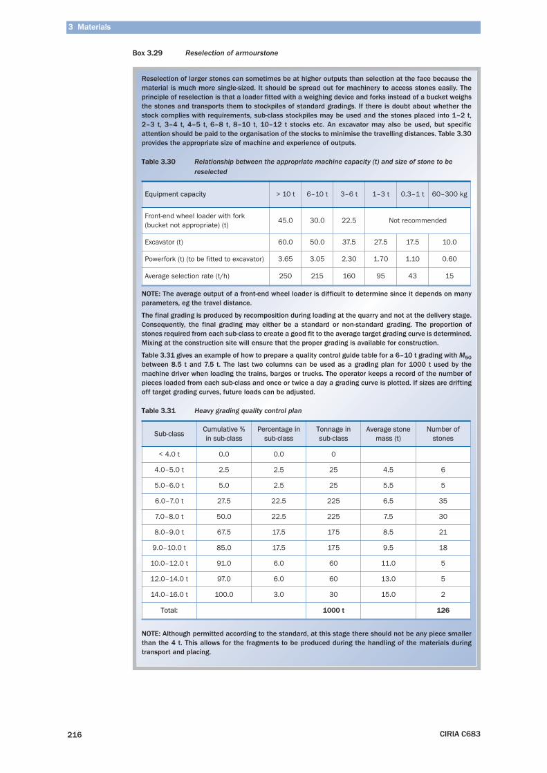
Box 3.29 Reselection of armourstone
Reselection of larger stones can sometimes be at higher outputs than selection at the face because thematerial is much more single-sized. It should be spread out for machinery to access stones easily. Theprinciple of reselection is that a loader fitted with a weighing device and forks instead of a bucket weighsthe stones and transports them to stockpiles of standard gradings. If there is doubt about whether thestock complies with requirements, sub-class stockpiles may be used and the stones placed into 1–2 t,2–3 t, 3–4 t, 4–5 t, 6–8 t, 8–10 t, 10–12 t stocks etc. An excavator may also be used, but specificattention should be paid to the organisation of the stocks to minimise the travelling distances. Table 3.30provides the appropriate size of machine and experience of outputs.
Table 3.30 Relationship between the appropriate machine capacity (t) and size of stone to bereselected
NOTE: The average output of a front-end wheel loader is difficult to determine since it depends on manyparameters, eg the travel distance.
The final grading is produced by recomposition during loading at the quarry and not at the delivery stage.Consequently, the final grading may either be a standard or non-standard grading. The proportion ofstones required from each sub-class to create a good fit to the average target grading curve is determined.Mixing at the construction site will ensure that the proper grading is available for construction.
Table 3.31 gives an example of how to prepare a quality control guide table for a 6–10 t grading with M50between 8.5 t and 7.5 t. The last two columns can be used as a grading plan for 1000 t used by themachine driver when loading the trains, barges or trucks. The operator keeps a record of the number ofpieces loaded from each sub-class and once or twice a day a grading curve is plotted. If sizes are driftingoff target grading curves, future loads can be adjusted.
Table 3.31 Heavy grading quality control plan
NOTE: Although permitted according to the standard, at this stage there should not be any piece smallerthan the 4 t. This allows for the fragments to be produced during the handling of the materials duringtransport and placing.
Equipment capacity > 10 t 6–10 t 3–6 t 1–3 t 0.3–1 t 60–300 kg
Front-end wheel loader with fork(bucket not appropriate) (t)
45.0 30.0 22.5 Not recommended
Excavator (t) 60.0 50.0 37.5 27.5 17.5 10.0
Powerfork (t) (to be fitted to excavator) 3.65 3.05 2.30 1.70 1.10 0.60
Average selection rate (t/h) 250 215 160 95 43 15
Sub-classCumulative %in sub-class
Percentage insub-class
Tonnage insub-class
Average stonemass (t)
Number ofstones
< 4.0 t 0.0 0.0 0
4.0–5.0 t 2.5 2.5 25 4.5 6
5.0–6.0 t 5.0 2.5 25 5.5 5
6.0–7.0 t 27.5 22.5 225 6.5 35
7.0–8.0 t 50.0 22.5 225 7.5 30
8.0–9.0 t 67.5 17.5 175 8.5 21
9.0–10.0 t 85.0 17.5 175 9.5 18
10.0–12.0 t 91.0 6.0 60 11.0 5
12.0–14.0 t 97.0 6.0 60 13.0 5
14.0–16.0 t 100.0 3.0 30 15.0 2
Total: 1000 t 126
3 Materials
CIRIA C683218
3 Materials
Quarry run. This category includes everything from the finest material of the quarry yieldup to a maximum size in the blastpile and is best described as 0–M kg. Consequently, theproduction simply consists of removing the oversize. This can easily be done with a wheelloader or an excavator. When using a wheel loader, the large size of the bucket and thelimited visibility of the driver will make it practically impossible to produce a lighter corematerial than 0–1000 kg. Using an excavator with a smaller bucket and digging towards thecabin could produce a 0–500 kg material. Note that the grading of the muckpile gets finerwhen digging deeper into it.
Processed core materials. This material is produced by removing both the oversized andfines, generally by means of a robust static grizzly (see Box 3.33). Due regard should be givento the lower cut-off value since it significantly affects the amount of by-product for which analternative use should be found. Changing the lower limit from 1 kg to 5 kg may effectivelylead to rejection of an extra 10 per cent of quarry yield (see also Section 3.4.4).
3.9.7.4 Technologies for the different selection or processing methods
This section presents different techniques or tools suitable for armourstone production,illustrated in Boxes 3.30–3.35 as follows:
� crusher (Box 3.30)
� selection hill (Box 3.31)
� trommel screen (Box 3.32)
� bars or static grizzly (Box 3.33)
� barsizer unit (Box 3.34)
� sidekick (Box 3.35).
Vibrating screens and grizzlies may be used for production of coarse grading armourstoneprovided they are sturdier than traditional aggregates screens. They can be located after theprimary crusher with possible adjustment of its characteristics to produced gradings withnominal upper limit up to 100 kg or 200 kg (see Box 3.30). This may be appropriate forproduction of gabion stone, for instance. The vibrating screen decks will need to be adaptedto handle the larger stones. Constraining the maximum feed size and the smallest mesh orhole opening will generally prevent damage. Typical limitations are given in Table 3.32.
Table 3.32 Limitation of screening device to limit damages
NOTE: It is easier to make round holes in a steel plate in a workshop than to make squareones. The diameter should be increased by 1.23 times the width of a square hole needed fora similar screening result. However, a steel plate with round holes has a lower screeningcapacity. Bigger screening areas and decks are therefore required for similar production rates.
Maximum feed size Minimum passing size
Grizzly ~ 120 kg ~ 100 mm (1.7 kg)
Holed steel plate ~ 200 mm (13.0 kg) 150 mm (5.6 kg)
Woven wire mesh ~ 125 mm (3.2 kg) 75 mm (0.7 kg)
3 Materials
CIRIA C683258
For existing structures, regular monitoring, at least after storms, should be carried out andbroken armour units may need to be replaced. Rather than repairing a Dolos armour layerthe US Army Corps of Engineers has developed the Core-loc, which can fulfil this role.
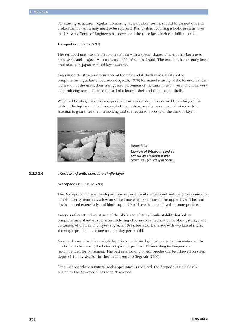
Tetrapod (see Figure 3.94)
The tetrapod unit was the first concrete unit with a special shape. This unit has been usedextensively and projects with units up to 50 m³ can be found. The tetrapod has recently beenused mostly in Japan in multi-layer systems.
Analysis on the structural resistance of the unit and its hydraulic stability led tocomprehensive guidance (Sotramer-Sogreah, 1978) for manufacturing of the formworks, thefabrication of the units, their storage and placement of the units in two layers. The formworkfor producing tetrapods is composed of a bottom shell and three lateral shells.
Wear and breakage have been experienced in several structures caused by rocking of theunits in the top layer. The placement of the units as per the recommended standards isessential to guarantee the interlocking and the required porosity of the armour layer.
3.12.2.4 Interlocking units used in a single layer
Accropode (see Figure 3.95)
The Accropode unit was developed from experience of the tetrapod and the observation thatdouble-layer systems may allow unwanted movements of units in the upper layer. This unithas been used extensively and blocks up to 20 m³ have been employed in some projects.
Analyses of structural resistance of the block and of its hydraulic stability has led tocomprehensive standards for manufacturing of formworks, fabrication of blocks, storage andplacement of units in one layer (Sogreah, 1988). Formwork is made with two lateral shells,allowing a production of one unit per day per mould.
Accropodes are placed in a single layer in a predefined grid whereby the orientation of theblocks has to be varied; the latter is typically specified. Various sling techniques arerecommended for placement. The best interlocking of Accropodes can be achieved on steepslopes (3:4 or 1:1.5). For further details see also Sogreah (2000).
For situations where a natural rock appearance is required, the Ecopode (a unit closelyrelated to the Accropode) has been developed.
Figure 3.94
Example of Tetrapods used asarmour on breakwater withcrown wall (courtesy M Scott)
3 Materials
CIRIA C683284
other, or from sheathed fibres where the outer coating has the lower melting point.Typical polymers used are polypropylene (PP) or high-density polyethylene (HDPE).
Figure 3.110 Non-woven geotextile (courtesy Geofabrics)
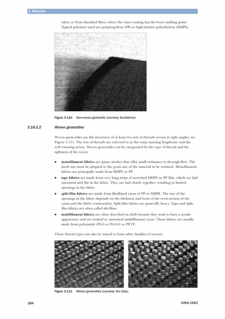
3.16.2.2 Woven geotextiles
Woven geotextiles are flat structures of at least two sets of threads woven at right angles; seeFigure 3.111. The sets of threads are referred to as the warp running lengthwise and theweft running across. Woven geotextiles can be categorised by the type of thread and thetightness of the weave.
� monofilament fabrics are gauze meshes that offer small resistance to through-flow. Themesh size must be adapted to the grain size of the material to be retained. Monofilamentfabrics are principally made from HDPE or PP
� tape fabrics are made form very long strips of stretched HDPE or PP film, which are laiduntwisted and flat in the fabric. They are laid closely together, resulting in limitedopenings in the fabric
� split-film fabrics are made from fibrillated yarns of PP or HDPE. The size of theopenings in the fabric depends on the thickness and form of the cross-section of theyarns and the fabric construction. Split-film fabrics are generally heavy. Tape and split-film fabrics are often called slit-films
� multifilament fabrics are often described as cloth because they tend to have a textileappearance and are twisted or untwisted multifilament yarns. These fabrics are usuallymade from polyamide (PA 6 or PA 6.6) or PETP.
These thread types can also be mixed to form other families of wovens.
Figure 3.111 Woven geotextiles (courtesy Ten Cate)
4 Physical site conditions and data collection
CIRIA C683326
place will be different and the typical neap tide (MHWN) timing is about six hours earlier orlater than the MHWS timing. When planning work on structures it is useful to know thetiming of the most extreme low waters and whether or not they occur during daylight.
For a detailed description of sea level fluctuations and tidal phenomena, see Pugh (1987).
4.2.2.3 Storm surges
Meteorological phenomena, namely atmospheric pressure and wind, may also affect the sealevel in particular during storm events. This section focuses on atmospheric pressure effectswhile wind effects are considered in the next section. Pressure and wind effects are oftencombined during storms generating long waves, called storm surges, with a characteristictime-scale of several hours to one day and a wavelength approximately equal to the width ofthe centre of the depression, typically 150–800 km. These storm surges produce significantvariations of the sea level, up to 2–3 m at the shore depending on the shape of the coastlineand the storm intensity. In practice, the term storm surge level is sometimes used loosely toinclude the astronomical tidal component and other meteorological effects.
Local low atmospheric pressures (depressions) cause corresponding rises in water level.Similarly, high pressures cause drops in water levels. This is the so-called inverse barometereffect.
For open water domains, Equation 4.9 gives the relationship between the static rise in waterlevel za (m) and the corresponding atmospheric pressure:
za = 0.01(1013 – pa) (4.9)
where pa = atmospheric pressure at sea level (hPa) and 1013 hPa is the pressure in normalconditions (see Section 4.2.1.2).
NOTE: Equation 4.9 results from simple equilibrium between the atmosphere and the oceanin static conditions. Where the atmospheric pressure is higher than the mean value of 1013 hPa, the sea level decreases, provided that it can increase at another place where theatmospheric pressure is lower than the mean value. This simple relationship does not applyfor closed domains of small dimensions such as lakes. Indeed, if the atmospheric pressure isthe same over the whole water domain there is no change in static water level.
Dynamic effects can cause a significant amplification of the rise in water level, however. Whenthe depression moves quickly, the water level rise follows the depression. The height of theselong waves may increase considerably as a result of shoaling in the nearshore zones. Alongthe coasts of the southern North Sea, storm surges with a height of 3 m have been recorded.
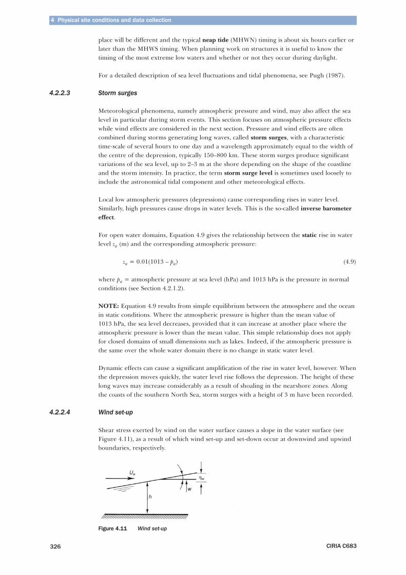
4.2.2.4 Wind set-up
Shear stress exerted by wind on the water surface causes a slope in the water surface (seeFigure 4.11), as a result of which wind set-up and set-down occur at downwind and upwindboundaries, respectively.
Figure 4.11 Wind set-up
4 Physical site conditions and data collection
CIRIA C683332
referred to as infra-gravity waves. If the waves approach a beach obliquely the long waves canmodify the longshore currents and also form edge waves that travel along the beach and areoften trapped within the nearshore zone. Long waves also produce variations in both the set-up and the run-up in the surf zone caused by the primary waves. The long-period oscillationsin these effects can cause both greater damage to, and overtopping of coastal structures.
An order of magnitude of the surf-beat amplitude in shallow water and in the surf zone canbe obtained by using Equation 4.23, an empirical formula derived by Goda (2000):
(4.23)
where ςrms = root-mean-square amplitude of the surf-beat profile (m). It is a function of theequivalent deep-water (significant) wave height H′o defined in Section 4.2.2.5 (m), the deep-water wavelength Lo (m) computed from the significant wave period Ts (see Section 4.2.4.4)as Lo = g (Ts)²/(2π), and the local water depth, h (m).
Bowers (1993) also provides formulae to estimate the amplitude of bound long waves forintermediate depths and also for surf beat significant wave height. For the case of coastalstructures exposed to long waves, Kamphuis (2001) proposed the use of Equation 4.24 toestimate the zero moment wave height of the long waves, Hm0LW , at the structure as a functionof the breaking significant wave height Hs,b and the peak wave period Tp (see Section 4.2.4.5).
(4.24)
Equation 4.24 can be approximated as a rule of thumb by (Hm0)LW = 0.4Hs,b . Kamphuis(2001) also addresses the problem of reflection of these long waves on coastal structures,showing that the long wave profile (with distance offshore) may be described as the sum of anabsorbed wave and a standing wave. The long wave reflection coefficient was about 22 percent during the set of experiments.
4.2.2.8 Tsunamis
Tsunamis are seismically induced gravity waves characterised by wave periods that are in theorder of minutes rather than seconds (typically 10–60 minutes). They often originate fromearthquakes below the ocean, where water depths can be more than 1000 m, and may travellong distances without reaching any noticeable wave height. However, when approachingcoastlines their height may increase considerably. Because of their large wavelength, thesewaves are subject to strong shoaling and refraction effects. Approaching from quite largewater depths, they can be calculated using shallow-water theory. Wave reflection from therelatively deep slopes of continental shelves may also be an important consideration.
Some theoretical work is available (eg Wilson, 1963), as well as numerical models to describetsunami generation, propagation and run-up over land areas (eg Shuto, 1991; Yeh et al,1994; Tadepalli and Synolakis, 1996) and also some large-scale experiments (eg Liu et al,1995). More information on tsunamis can be obtained from the Internet, for example at<www.pmel.noaa.gov/tsunami>.
Tsunamis are as unpredictable as earthquakes. Figure 4.15 presents observations for heightand period of tsunamis from Japanese sources observed at coasts within a range of about 750km from the epicentre of sub-ocean earthquakes.
ς rms
oHHL
hH'
.'
'
/
0
0
0
1 2
0 01 1= +⎛
⎝⎜⎜
⎞
⎠⎟⎟
⎡
⎣⎢⎢
⎤
⎦⎥⎥
−
H
HH
gTm LW
s b
s b
p
0
2
0 24
0 11( )
=⎡
⎣⎢⎢
⎤
⎦⎥⎥
−
,
,
.
.
CIRIA C683 343
4.2 Hydraulic boundary conditions and data collection – marine and coastal waters
� the upstream discharge.
In the case of tidal motion the physical laws reduce to the so-called long wave equations,based on the assumption that vertical velocities and accelerations are negligible. Dependingon the type of estuary, the long wave equations may be further simplified.
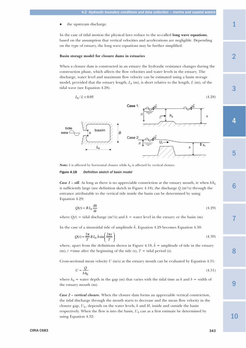
Basin storage model for closure dams in estuaries
When a closure dam is constructed in an estuary the hydraulic resistance changes during theconstruction phase, which affects the flow velocities and water levels in the estuary. Thedischarge, water level and maximum flow velocity can be estimated using a basin storagemodel, provided that the estuary length, Lb (m), is short relative to the length, L (m), of thetidal wave (see Equation 4.28).
(4.28)
Note: b is affected by horizontal closure while h0 is affected by vertical closure.
Figure 4.18 Definition sketch of basin model
Case 1 – sill. As long as there is no appreciable constriction at the estuary mouth, ie when b/hbis sufficiently large (see definition sketch in Figure 4.18), the discharge Q (m³/s) through theentrance attributable to the vertical tide inside the basin can be determined by usingEquation 4.29:
(4.29)
where Q(t) = tidal discharge (m³/s) and h = water level in the estuary or the basin (m).
In the case of a sinusoidal tide of amplitude h, Equation 4.29 becomes Equation 4.30:
(4.30)
where, apart from the definitions shown in Figure 4.18, h = amplitude of tide in the estuary(m), t =time after the beginning of the tide (s), T = tidal period (s).
Cross-sectional mean velocity U (m/s) at the estuary mouth can be evaluated by Equation 4.31:
(4.31)
where h0 = water depth in the gap (m) that varies with the tidal time as h and b = width ofthe estuary mouth (m).
Case 2 – vertical closure. When the closure dam forms an appreciable vertical constriction,the tidal discharge through the mouth starts to decrease and the mean flow velocity in theclosure gap, U0 , depends on the water levels, h and H, inside and outside the basinrespectively. When the flow is into the basin, U0 can as a first estimate be determined byusing Equation 4.32:
ˆ
L Lb / .< 0 05
Q t B L htb( ) = d
d
Q tT
B L h tTb( ) sin= ⎛
⎝⎜⎞⎠⎟
2 2π π
U Qbh
=0
ˆ
1
3
4
10
9
8
7
6
5
2
ˆ
(4.32)
where H = sea-side water level above the dam crest (m) and hb = water level in the basinabove the dam crest (m).
Further discussion of discharge and velocity through the gap is given in Section 5.1.2.3where discharge coefficients are introduced to improve precision. A simple model to calculatethe response water level of the basin, h, given the tide at the seaward side as the boundarycondition, H(t), is based upon Equation 4.33, which results from the combination ofEquations 4.29, 4.31 and 4.32:
(4.33)
where Qriver = river discharge into the basin (m³/s), if relevant, h0 = water depth on the crest ofthe closure dam (m) (see Section 5.1.2.3) and H, hb and b are defined according to Figure 4.18.
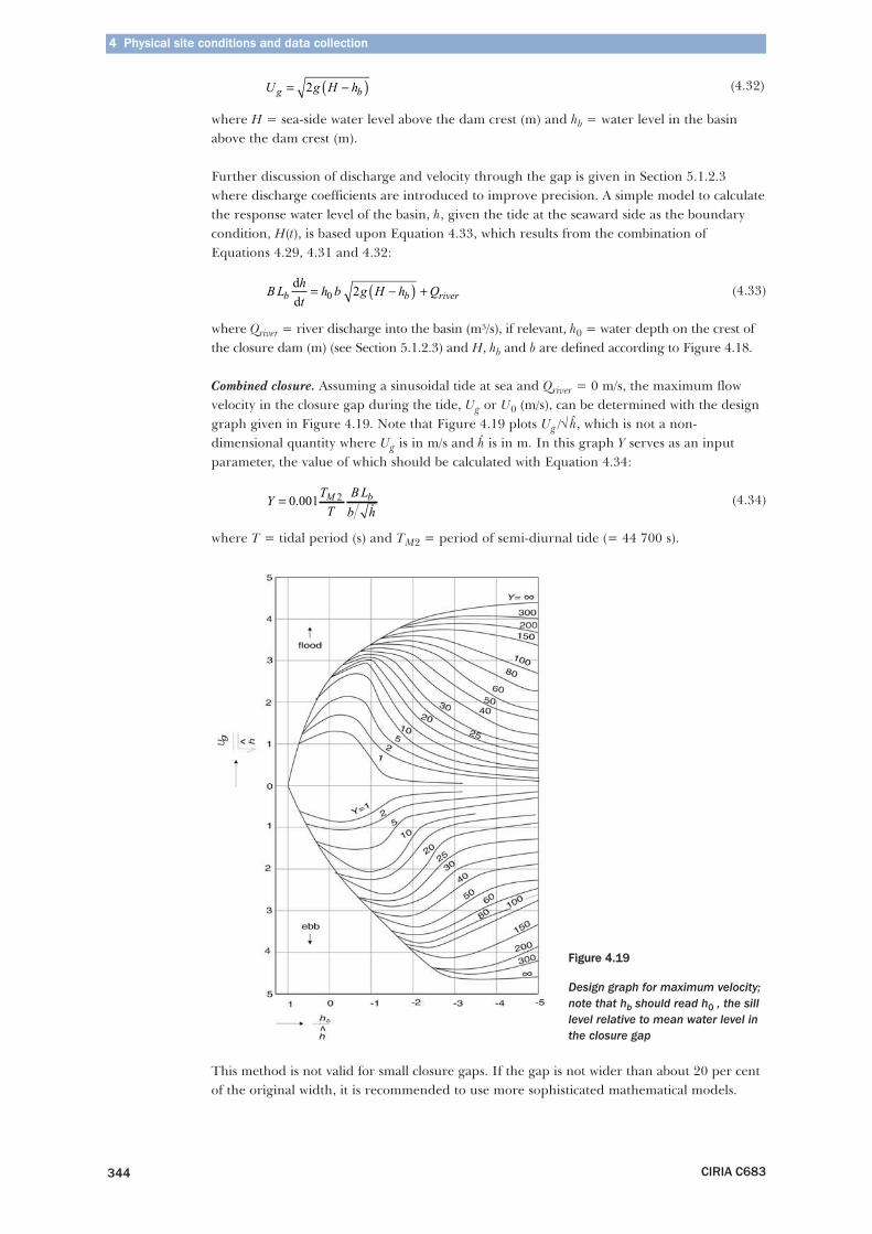
Combined closure. Assuming a sinusoidal tide at sea and Qriver = 0 m/s, the maximum flowvelocity in the closure gap during the tide, Ug or U0 (m/s), can be determined with the designgraph given in Figure 4.19. Note that Figure 4.19 plots Ug /√h, which is not a non-dimensional quantity where Ug is in m/s and h is in m. In this graph Y serves as an inputparameter, the value of which should be calculated with Equation 4.34:
(4.34)
where T = tidal period (s) and TM2 = period of semi-diurnal tide (= 44 700 s).
This method is not valid for small closure gaps. If the gap is not wider than about 20 per centof the original width, it is recommended to use more sophisticated mathematical models.
4 Physical site conditions and data collection
CIRIA C683344
B L ht
h b g H h Qb b riverd
d= −( ) +0 2
ˆˆ
Y TT
B Lb h
M b= 0 001 2.
Figure 4.19
Design graph for maximum velocity;note that hb should read h0 , the silllevel relative to mean water level inthe closure gap
U g H hg b= −( )2
ˆ
4 Physical site conditions and data collection
CIRIA C683350
equation accurately whenever necessary, but explicit approximations, such as given in Box 4.3, can also be used.
The propagation velocity of wave crests (phase speed) is c = L/T = ω /k (m/s) and thepropagation velocity of energy (group velocity) is given by cg = ∂ω/∂k (m/s). In linear wavetheory, based on Equation 4.38, the expressions for phase and group velocity are given byEquations 4.39 and 4.40 respectively.
(4.39)
(4.40)
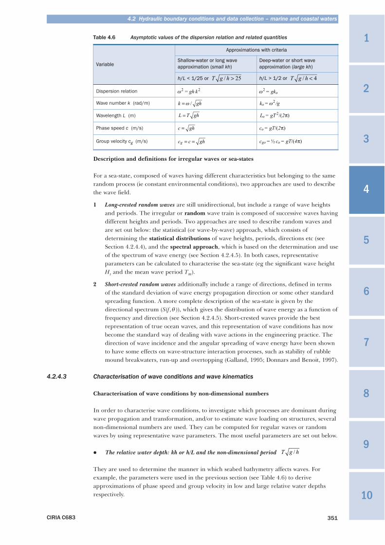
Note that the factor n has two asymptotic values: (1) when the relative water depth, kh (-), issmall, n tends towards 1; (2) when kh is large n tends towards ½; in this case the wave energypropagates at a speed that is half of that of individual waves. For these asymptotic cases,particular expressions of k, L, c and cg may be derived analytically and are listed in Table 4.6,together with the non-dimensional criteria for using these approximations. For values indeep water (large value of kh), the subscript “0” or “o” was used conventionally (eg Lo for thedeep-water wavelength). Here the latter, “o” (of offshore), is used. From Table 4.6 it shouldbe noted, for example, that in shallow-water conditions, c and cg do not depend any more onthe wave period, T, and that all waves have the same velocity (non-dispersive waves), which,in this case, equals the velocity of energy.
Box 4.3 Explicit approximations of the linear dispersion relation for water waves
c g k h gk
k h= ( ) = ( )ω
tanh tanh
c nc n k hk hg = = + ( )
⎛
⎝⎜⎜
⎞
⎠⎟⎟with
1
21
2
2sinh
There are numerous approximations of the dispersion relation given by Equation 4.38. Equation 4.41 givesthe rational one proposed by Hunt (1979) at order 9, which is very accurate (always less than 0.01 percent of relative error in kh):
(4.41)
where ko = 2π/Lo = ω2/g = deep-water wave number (rad/m) and the values of an are as follows:
a1 = 0.66667 a2 = 0.35550 a3 = 0.16084 a4 = 0.06320 a5 = 0.02174a6 = 0.00654 a7 = 0.00171 a8 = 0.00039 a9 = 0.00011.
Hunt (1979) also provides a similar formula at order 6, with a relative error in kh always less than 0.2 percent.
Alternatively, the simpler explicit formulation by Fenton and McKee (1990) (see Equation 4.42) can beused. Although it is less accurate than the former (1.5 per cent of maximum relative error), it is easier touse on a calculator.
or equivalent: (4.42)
Other explicit expressions have been proposed by Eckart (1952), Wu and Thornton (1986), Guo (2002).
k h k hk h
a k ho
o
n on
n
( ) = ( ) +
+ ( )=
∑2 2
1
9
1
kg
hg
=⎛
⎝⎜⎜
⎞
⎠⎟⎟
⎡
⎣
⎢⎢⎢
⎤
⎦
⎥⎥⎥
⎧⎨⎪
⎩⎪
⎫⎬⎪
⎭⎪
ωω
23 2
2 3
coth
//
L L k ho o= ( )⎡⎣⎢
⎤⎦⎥{ }tanh
//
3 42 3
CIRIA C683 351
4.2 Hydraulic boundary conditions and data collection – marine and coastal waters
Table 4.6 Asymptotic values of the dispersion relation and related quantities
Description and definitions for irregular waves or sea-states
For a sea-state, composed of waves having different characteristics but belonging to the samerandom process (ie constant environmental conditions), two approaches are used to describethe wave field.
1 Long-crested random waves are still unidirectional, but include a range of wave heightsand periods. The irregular or random wave train is composed of successive waves havingdifferent heights and periods. Two approaches are used to describe random waves andare set out below: the statistical (or wave-by-wave) approach, which consists ofdetermining the statistical distributions of wave heights, periods, directions etc (seeSection 4.2.4.4), and the spectral approach, which is based on the determination and useof the spectrum of wave energy (see Section 4.2.4.5). In both cases, representativeparameters can be calculated to characterise the sea-state (eg the significant wave heightHs and the mean wave period Tm).
2 Short-crested random waves additionally include a range of directions, defined in termsof the standard deviation of wave energy propagation direction or some other standardspreading function. A more complete description of the sea-state is given by thedirectional spectrum (S(f,θ )), which gives the distribution of wave energy as a function offrequency and direction (see Section 4.2.4.5). Short-crested waves provide the bestrepresentation of true ocean waves, and this representation of wave conditions has nowbecome the standard way of dealing with wave actions in the engineering practice. Thedirection of wave incidence and the angular spreading of wave energy have been shownto have some effects on wave-structure interaction processes, such as stability of rubblemound breakwaters, run-up and overtopping (Galland, 1995; Donnars and Benoit, 1997).
4.2.4.3 Characterisation of wave conditions and wave kinematics
Characterisation of wave conditions by non-dimensional numbers
In order to characterise wave conditions, to investigate which processes are dominant duringwave propagation and transformation, and/or to estimate wave loading on structures, severalnon-dimensional numbers are used. They can be computed for regular waves or randomwaves by using representative wave parameters. The most useful parameters are set out below.
� The relative water depth: kh or h/L and the non-dimensional period
They are used to determine the manner in which seabed bathymetry affects waves. Forexample, the parameters were used in the previous section (see Table 4.6) to deriveapproximations of phase speed and group velocity in low and large relative water depthsrespectively.
Variable
Approximations with criteria
Shallow-water or long waveapproximation (small kh)
Deep-water or short waveapproximation (large kh)
h/L < 1/25 or h/L > 1/2 or
Dispersion relation
Wave number k (rad/m)
Wavelength L (m)
Phase speed c (m/s)
Group velocity cg (m/s)
T g h/ > 25 T g h/ < 4
c gh=
L T gh=
k gh= ω /
c c ghg = =
T g h/
ω2 2 = gh k
c = gT 2o /( )π
L = gT 2o2/( )π
k = /go ω2
c = c = gT 4go o½ /( )π
ω2 = gko
1
3
4
10
9
8
7
6
5
2
4 Physical site conditions and data collection
CIRIA C683352
� The wave steepness s = H/L and the relative wave height H/h
They are measures of non-linearity of the wave (see Figure 4.23). They are used in particularto quantify the importance of non-linear effects and they appear in the formation of criteriafor predicting wave breaking. A specific use of the wave steepness is made if the wave heightis taken at the toe of the structure and the wavelength in deep water. In fact this is a fictitiouswave steepness so = H/Lo and is often used in design formulae for structures. The main goalin this case is not to describe the wave steepness itself, but to include the effect of the waveperiod on structure response through Lo = gT2/(2π), which is only valid offshore.
� The Ursell number U (-)
This is a combination of the former numbers and is presented in Equation 4.43. It is used tocharacterise the degree of non-linearity of the waves.
(4.43)
� The surf similarity parameter ξ , also known as the Iribarren number, Ir (see Equation 4.44)
This is used for the characterisation of many phenomena related to waves in shallow water,such as wave breaking, run-up and overtopping. It reflects the ratio of bed slope andfictitious wave steepness, so.
(4.44)
When the deep-water wave height, Ho, is used instead of H, this number is denoted ξo or Iro .
This parameter is often used for beaches, and often for design of structures too. It gives thetype of wave breaking and wave load on the structure. Actually, waves can break first on thedepth-limited foreshore before reaching the structure and then break once again on to thestructure. On the foreshore the breaker type is generally spilling, sometimes plunging. Onthe structure itself it is never spilling, but plunging (gentle structure slope), surging orcollapsing (see Section 4.2.4.7 for the definition of breaker types).
When using these parameters for random waves, it should be stressed and indicated (as asubscript of these parameters, for example) which characteristic wave height and period arebeing used in their evaluation (eg subscript “p” if the peak period Tp is used, and “m” if themean period Tm is used).
For further discussion on the use and the notation of ξ, please also refer to Section 5.1.1.1.
Overview of methods for computing wave kinematics
Many wave theories are available to derive other wave parameters and kinematics (velocities,accelerations, pressure etc) from the above-mentioned basic parameters (eg H and T, pluspossibly a flow speed). The majority of design methods are based on Stokes linear wavetheory (ie small amplitude wave theory) derived for a flat bottom (ie constant water depth). Amajor advantage of linear theory in design procedures is that the principle of superpositioncan be applied to wave-related data, obtained from a composite wave field. Using linear wavetheory, practical engineering approximations can be derived for regular waves propagatingin deep and shallow water respectively (see Table 4.6). Expressions for orbital velocities ux , uy ,uz and pressure p are presented below as Equations 4.45 to 4.48 for the case of a regularwave with a height H, period T (angular frequency ω = 2π/T) and direction θ with respect to
U H Lh
Hh
hL
= = ⎛⎝⎜
⎞⎠⎟
⎛⎝⎜
⎞⎠⎟
2
3
2
ξα α α= = =
( ) ( )tan tan
/
tan
s H L H gTo o 2 2π
4 Physical site conditions and data collection
CIRIA C683356
Distribution of individual wave heights in a sea-state
During each sea-state a (short-term) distribution of wave heights applies. Once thedistribution function of wave heights is known, all the characteristic wave heights listed inTable 4.7 can be computed. Some basic and important results for wave distributions aresummarised below: first for the deep-water case, and then for the shallow-water case. Thelatter is more important for the design of coastal structures, but also more difficult to modeland parameterise.
� Distribution of deep-water wave heights
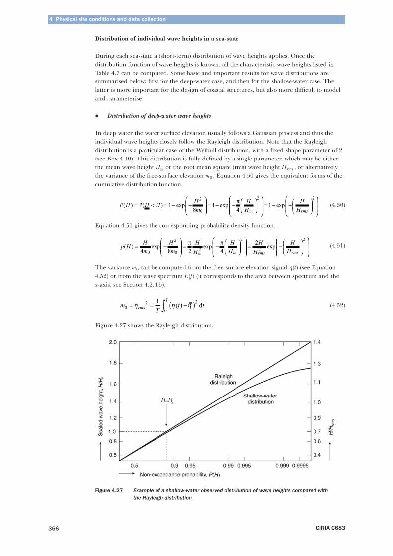
In deep water the water surface elevation usually follows a Gaussian process and thus theindividual wave heights closely follow the Rayleigh distribution. Note that the Rayleighdistribution is a particular case of the Weibull distribution, with a fixed shape parameter of 2(see Box 4.10). This distribution is fully defined by a single parameter, which may be eitherthe mean wave height Hm or the root mean square (rms) wave height Hrms , or alternativelythe variance of the free-surface elevation m0 . Equation 4.50 gives the equivalent forms of thecumulative distribution function.
(4.50)
Equation 4.51 gives the corresponding probability density function.
(4.51)
The variance m0 can be computed from the free-surface elevation signal η(t) (see Equation4.52) or from the wave spectrum E(f) (it corresponds to the area between spectrum and thex-axis, see Section 4.2.4.5).
(4.52)
Figure 4.27 shows the Rayleigh distribution.
Figure 4.27 Example of a shallow-water observed distribution of wave heights compared with the Rayleigh distribution
P H H H Hm
HHm
( ) ( ) exp exp= < = − −⎛
⎝⎜⎜
⎞
⎠⎟⎟ = − − ⎛
⎝⎜
⎞⎠⎟
⎛
⎝⎜⎜
⎞
⎠⎟⎟
P 18
14
2
0
2π == − −⎛⎝⎜
⎞⎠⎟
⎛
⎝⎜⎜
⎞
⎠⎟⎟
1
2
expH
Hrms
p H Hm
Hm
HH
HHm m
( ) exp exp= −⎛
⎝⎜⎜
⎞
⎠⎟⎟ = − ⎛
⎝⎜
⎞⎠⎟
⎛
⎝⎜⎜
⎞
⎠⎟⎟
=4 8 2 40
2
02
2π π 222
2HH
HHrms rms
exp −⎛⎝⎜
⎞⎠⎟
⎛
⎝⎜⎜
⎞
⎠⎟⎟
mT
t trmsT
02 2
0
1= = −( )∫η η η( ) d
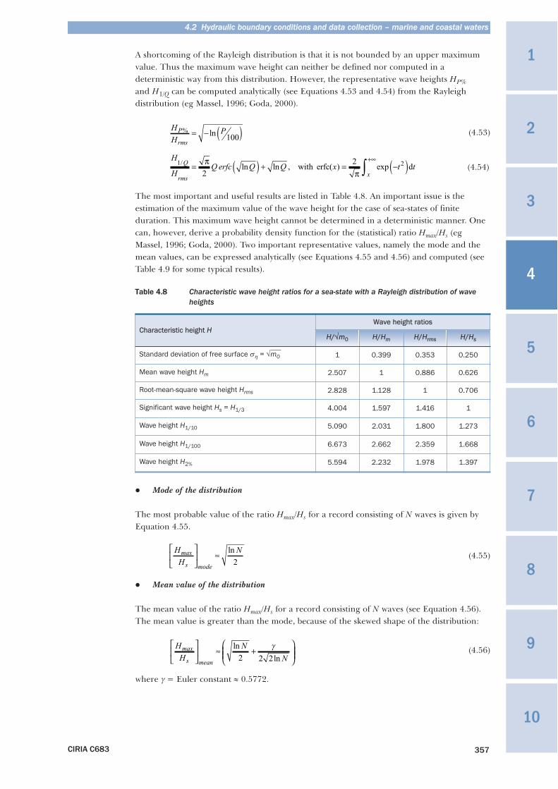
A shortcoming of the Rayleigh distribution is that it is not bounded by an upper maximumvalue. Thus the maximum wave height can neither be defined nor computed in adeterministic way from this distribution. However, the representative wave heights HP%and H1/Q can be computed analytically (see Equations 4.53 and 4.54) from the Rayleighdistribution (eg Massel, 1996; Goda, 2000).
(4.53)
(4.54)
The most important and useful results are listed in Table 4.8. An important issue is theestimation of the maximum value of the wave height for the case of sea-states of finiteduration. This maximum wave height cannot be determined in a deterministic manner. Onecan, however, derive a probability density function for the (statistical) ratio Hmax/Hs (egMassel, 1996; Goda, 2000). Two important representative values, namely the mode and themean values, can be expressed analytically (see Equations 4.55 and 4.56) and computed (seeTable 4.9 for some typical results).
Table 4.8 Characteristic wave height ratios for a sea-state with a Rayleigh distribution of waveheights
� Mode of the distribution
The most probable value of the ratio Hmax/Hs for a record consisting of N waves is given byEquation 4.55.
(4.55)
� Mean value of the distribution
The mean value of the ratio Hmax/Hs for a record consisting of N waves (see Equation 4.56).The mean value is greater than the mode, because of the skewed shape of the distribution:
(4.56)
where γ = Euler constant ≈ 0.5772.
CIRIA C683 357
4.2 Hydraulic boundary conditions and data collection – marine and coastal waters
HH
PP
rms
% ln= − ( )100
H
HQ erfc Q Q x t tQ
rms x
1 2
2
2/ln ln , erfc( ) exp= ( ) + = −( )+∞
∫ππ
with d
HH
Nmax
s mode
⎡
⎣⎢
⎤
⎦⎥ ≈ ln
2
HH
NN
max
s mean
⎡
⎣⎢
⎤
⎦⎥ ≈ +
⎛
⎝⎜⎜
⎞
⎠⎟⎟
ln
ln2 2 2
γ
Characteristic height HWave height ratios
H/√m0 H/Hm H/Hrms H/Hs
Standard deviation of free surface ση = √m0 1 0.399 0.353 0.250
Mean wave height Hm 2.507 1 0.886 0.626
Root-mean-square wave height Hrms 2.828 1.128 1 0.706
Significant wave height Hs = H1/3 4.004 1.597 1.416 1
Wave height H1/10 5.090 2.031 1.800 1.273
Wave height H1/100 6.673 2.662 2.359 1.668
Wave height H2% 5.594 2.232 1.978 1.397
1
3
4
10
9
8
7
6
5
2
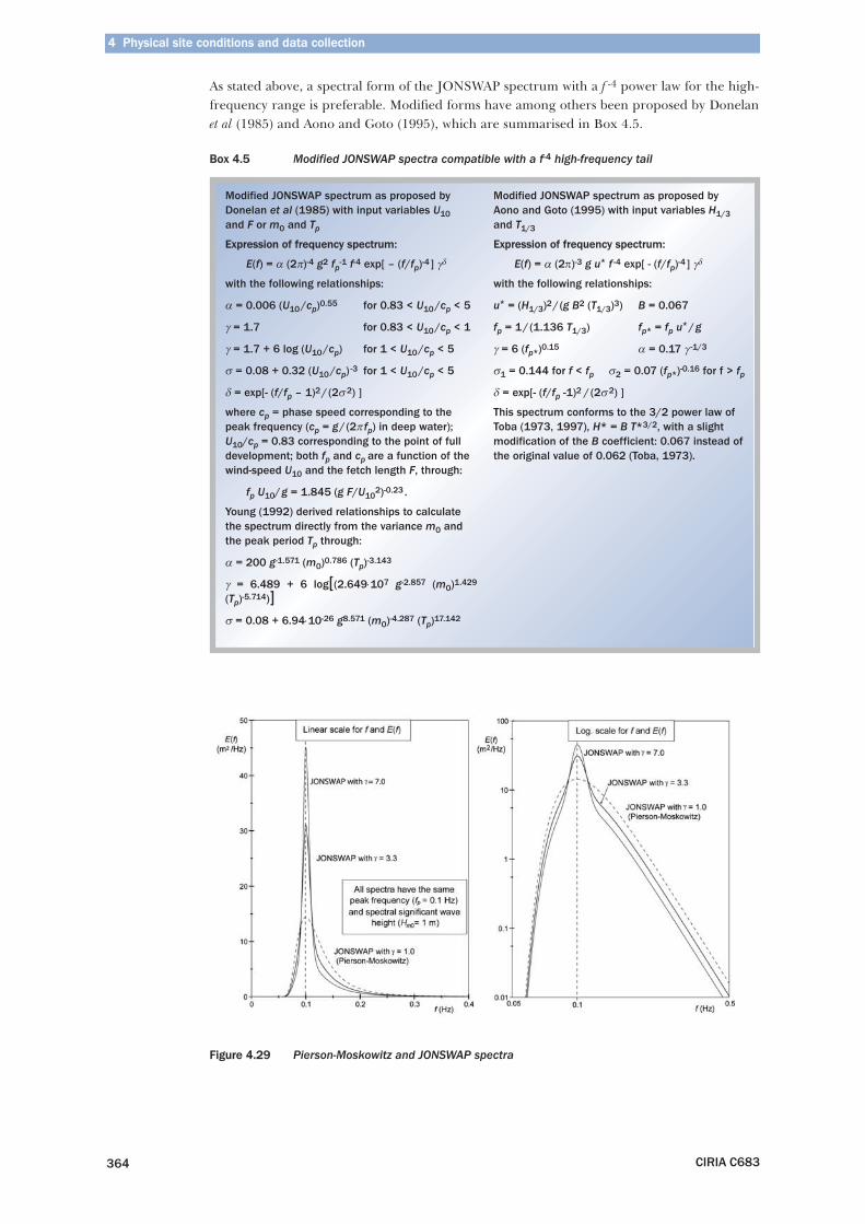
As stated above, a spectral form of the JONSWAP spectrum with a f -4 power law for the high-frequency range is preferable. Modified forms have among others been proposed by Donelanet al (1985) and Aono and Goto (1995), which are summarised in Box 4.5.
Box 4.5 Modified JONSWAP spectra compatible with a f-4 high-frequency tail
Figure 4.29 Pierson-Moskowitz and JONSWAP spectra
4 Physical site conditions and data collection
CIRIA C683364
Modified JONSWAP spectrum as proposed byDonelan et al (1985) with input variables U10and F or m0 and Tp
Expression of frequency spectrum:
E(f) = α (2π)-4 g2 fp-1 f-4 exp[ – (f/fp)-4 ] γδ
with the following relationships:
α = 0.006 (U10/cp)0.55 for 0.83 < U10/cp < 5
γ = 1.7 for 0.83 < U10/cp < 1
γ = 1.7 + 6 log (U10/cp) for 1 < U10/cp < 5
σ = 0.08 + 0.32 (U10/cp) -3 for 1 < U10/cp < 5
δ = exp[- (f/fp – 1)2/(2σ2) ]
where cp = phase speed corresponding to thepeak frequency (cp = g/(2π fp) in deep water);U10/cp = 0.83 corresponding to the point of fulldevelopment; both fp and cp are a function of thewind-speed U10 and the fetch length F, through:
fp U10/g = 1.845 (g F/U102)-0.23 .
Young (1992) derived relationships to calculatethe spectrum directly from the variance m0 andthe peak period Tp through:
α = 200 g-1.571 (m0)0.786 (Tp)-3.143
γ = 6.489 + 6 log[(2.649⋅107 g-2.857 (m0)1.429
(Tp)-5.714)]σ = 0.08 + 6.94⋅10-26 g8.571 (m0)-4.287 (Tp)17.142
Modified JONSWAP spectrum as proposed byAono and Goto (1995) with input variables H1/3and T1/3
Expression of frequency spectrum:
E(f) = α (2π)-3 g u* f -4 exp[ - (f/fp)-4 ] γδ
with the following relationships:
u* = (H1/3)2/(g B2 (T1/3)3) B = 0.067
fp = 1/(1.136 T1/3) fp* = fp u*/g
γ = 6 (fp*)0.15 α = 0.17 γ -1/3
σ1 = 0.144 for f < fp σ2 = 0.07 (fp*)-0.16 for f > fp
δ = exp[- (f/fp -1)2 /(2σ2) ]
This spectrum conforms to the 3/2 power law ofToba (1973, 1997), H* = B T*3/2, with a slightmodification of the B coefficient: 0.067 instead ofthe original value of 0.062 (Toba, 1973).
(4.87)
(4.88)
The value of the directional fetch, Fθ , is limited by the criterion expressed by Equation 4.89to avoid over-development of wave energy.
(4.89)
At this value of non-dimensional directional fetch, Fθ , fully development of waves is reached,resulting in Equations 4.90 and 4.91.
(4.90)
(4.91)
(c) Young and Verhagen method
Young and Verhagen (1996) analysed a large set of wave measurements performed on LakeGeorge (Australia). From this comprehensive dataset they were able to propose waveprediction formulae including both the effect of fetch F and water depth h (see Equations4.92 and 4.93). The formulae are based on the form of the formulae of SPM (1984) for wavegeneration in finite water depth:
(4.92)
.
(4.93)
This latter method offers the advantage of taking account of the actual water depth, which isimportant for reservoirs. Indeed, the mean water level in a reservoir may changesignificantly over a year leading to significant variations of fetch length and water depth.Both these parameters are present is the above formulae.
Later Young (1997) observed that these formulae fail to correctly model the wave height forshort fetches, which was attributed to the fact that the formulae revert to JONSWAPformulae (Hasselmann et al, 1973) for such cases. For a better treatment of this case, heproposed an equation that has to be integrated numerically to obtain a wave growth curve.
4.2 Hydraulic boundary conditions and data collection – marine and coastal waters
CIRIA C683 373
gT
Ug F
U
p
w w1010
2
0 23
0 542cos
.
cos
.
θ φ θ φ
θ
−( )=
−( )( )⎛
⎝
⎜⎜⎜
⎞
⎠
⎟⎟⎟
g tU
g F
U
min
w w1010
2
0 77
30 1cos
.
cos
.
θ φ θ φ
θ
−( )=
−( )( )⎛
⎝
⎜⎜⎜
⎞
⎠
⎟⎟⎟
gF
U w
θ
θ φ10
2
49 47 10
cos
.
−( )( )≤ ⋅
gH
U
s
w10
20 285
cos
.
θ φ−( )( )=
gTU
p
w10
7 56cos
.θ φ−( )
=
gHU
A BA
s
102 1
1
1
0 87
0 241= ⎛⎝⎜
⎞⎠⎟
⎛
⎝⎜
⎞
⎠⎟. tanh tanh
tanh
.
where:
where:
A ghU
1
102
0 75
0 493=⎛
⎝⎜⎜
⎞
⎠⎟⎟
.
.
B gFU
1
102
0 57
0 00313=⎛
⎝⎜⎜
⎞
⎠⎟⎟
.
.
gTU
A BA
p
102 2
2
2
0 37
7 519= ⎛⎝⎜
⎞⎠⎟
⎛
⎝⎜
⎞
⎠⎟. tanh tanh
tanh
.
A ghU
2
102
1 01
0 331=⎛
⎝⎜⎜
⎞
⎠⎟⎟
.
.
B gFU
2
102
0 73
0 0005215=⎛
⎝⎜⎜
⎞
⎠⎟⎟
.
.
and .
and
1
3
4
10
9
8
7
6
5
2
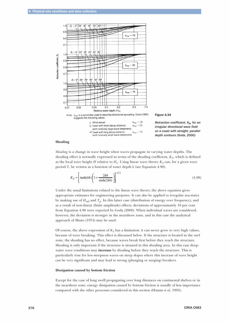
Shoaling
Shoaling is a change in wave height when waves propagate in varying water depths. Theshoaling effect is normally expressed in terms of the shoaling coefficient, KS, which is definedas the local wave height H relative to Ho. Using linear wave theory KS can, for a given waveperiod T, be written as a function of water depth h (see Equation 4.98).
(4.98)
Under the usual limitations related to the linear wave theory, the above equation givesappropriate estimates for engineering purposes. It can also be applied to irregular sea-statesby making use of Hm0 and Tp. In this latter case (distribution of energy over frequency), andas a result of non-linear (finite amplitude) effects, deviations of approximately 10 per centfrom Equation 4.98 were reported by Goda (2000). When individual waves are considered,however, the deviation is stronger in the nearshore zone, and in this case the analyticalapproach of Shuto (1974) may be used.
Of course, the above expression of KS has a limitation: it can never grow to very high values,because of wave breaking. This effect is discussed below. If the structure is located in the surfzone, the shoaling has no effect, because waves break first before they reach the structure.Shoaling is only important if the structure is situated in this shoaling area. In this case deep-water wave conditions may increase by shoaling before they reach the structure. This isparticularly true for low-steepness waves on steep slopes where this increase of wave heightcan be very significant and may lead to strong (plunging or surging) breakers.
Dissipation caused by bottom friction
Except for the case of long swell propagating over long distances on continental shelves or inthe nearshore zone, energy dissipation caused by bottom friction is usually of less importancecompared with the other processes considered in this section (Hamm et al, 1993).
4 Physical site conditions and data collection
CIRIA C683376
K kh khkhS = +
⎛
⎝⎜
⎞
⎠⎟
⎡
⎣⎢⎢
⎤
⎦⎥⎥
−
tanh( )sinh( )
12
2
1 2
Figure 4.34
Retraction coefficient, KR, for anirregular directional wave fieldon a coast with straight, paralleldepth contours (Goda, 2000)
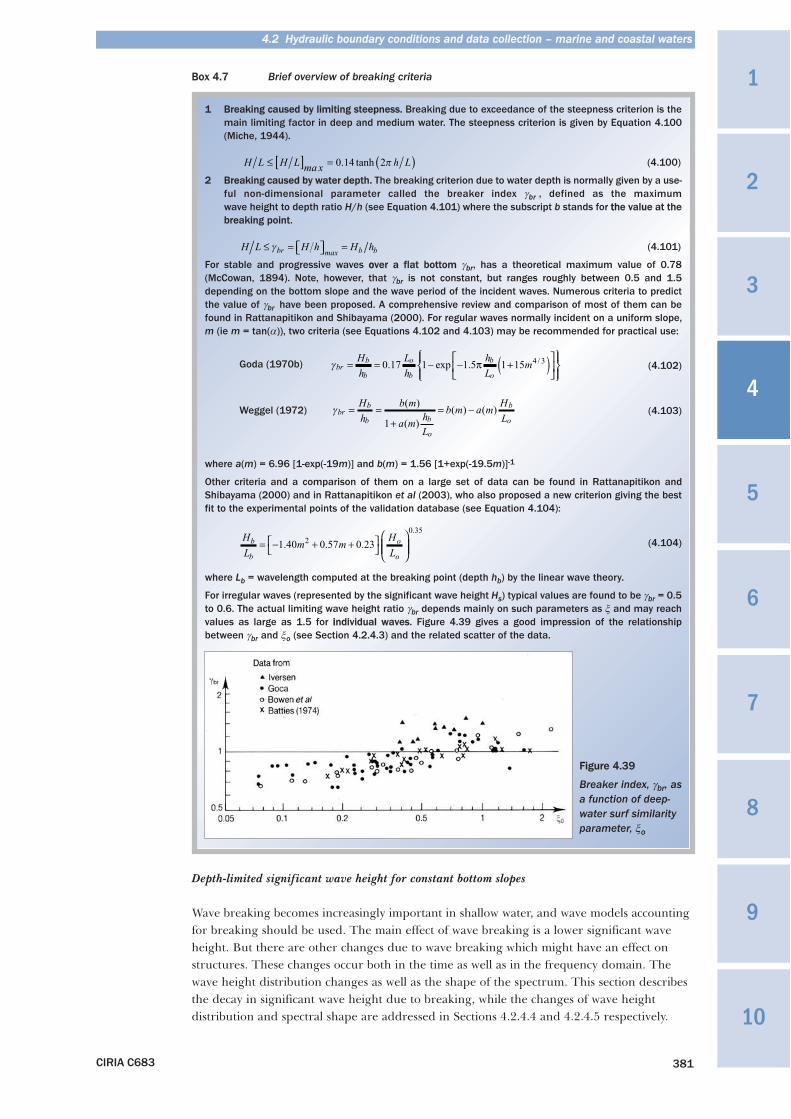
Box 4.7 Brief overview of breaking criteria
Depth-limited significant wave height for constant bottom slopes
Wave breaking becomes increasingly important in shallow water, and wave models accountingfor breaking should be used. The main effect of wave breaking is a lower significant waveheight. But there are other changes due to wave breaking which might have an effect onstructures. These changes occur both in the time as well as in the frequency domain. Thewave height distribution changes as well as the shape of the spectrum. This section describesthe decay in significant wave height due to breaking, while the changes of wave heightdistribution and spectral shape are addressed in Sections 4.2.4.4 and 4.2.4.5 respectively.
4.2 Hydraulic boundary conditions and data collection – marine and coastal waters
CIRIA C683 381
1 Breaking caused by limiting steepness. Breaking due to exceedance of the steepness criterion is themain limiting factor in deep and medium water. The steepness criterion is given by Equation 4.100(Miche, 1944).
(4.100)
2 Breaking caused by water depth. The breaking criterion due to water depth is normally given by a use-ful non-dimensional parameter called the breaker index γbr , defined as the maximum wave height to depth ratio H/h (see Equation 4.101) where the subscript b stands for tthe value at thebreaking point.
(4.101)
For stable and progressive waves oover a flat bottom γbr, has a theoretical maximum value of 0.78(McCowan, 1894). Note, however, that γbr is not constant, but ranges roughly between 0.5 and 1.5depending on the bottom slope and the wave period of the incident waves. Numerous criteria to predictthe value of γbr have been proposed. A comprehensive review and comparison of most of them can befound in Rattanapitikon and Shibayama (2000). For regular waves normally incident on a uniform slope,m (ie m = tan(α)), two criteria (see Equations 4.102 and 4.103) may be recommended for practical use:
(4.102)
(4.103)
where a(m) = 6.96 [1-exp(-19m)] and b(m) = 1.56 [1+exp(-19.5m)]-1
Other criteria and a comparison of them on a large set of data can be found in Rattanapitikon andShibayama (2000) and in Rattanapitikon et al (2003), who also proposed a new criterion giving the bestfit to the experimental points of the validation database (see Equation 4.104):
(4.104)
where Lb = wavelength computed at the breaking point (depth hb) by the linear wave theory.
For irregular waves (represented by the significant wave height Hs) typical values are found to be γbr = 0.5to 0.6. The actual limiting wave height ratio γbr depends mainly on such parameters as ξ and may reachvalues as large as 1.5 for iindividual waves. Figure 4.39 gives a good impression of the relationshipbetween γbr and ξo (see Section 4.2.4.3) and the related scatter of the data.
γbrb
b b
o
b
o
Hh
b m
a m hL
b m a m HL
= =+
= −( )
( )
( ) ( )
1
Goda (1970b)
Weggel (1972)
HL
m mHL
b
b
o
o= − + +⎡
⎣⎤⎦
⎛
⎝⎜⎜
⎞
⎠⎟⎟1 40 0 57 0 232
0 35
. . .
.
γbr = = − − +( )⎡⎣⎢
⎤⎦⎥
⎧⎨⎪
⎩⎪
⎫⎬⎪
⎭⎪Hh
Lh
hL
mb
b
o
b
b
o0 17 1 1 5 1 15 4 3. exp . /π
H L H L ma x h L≤ =[ ] ( )0 14 2. tanh π
H L H h H hbr max b b≤ = ⎡⎣ ⎤⎦ =γ
Figure 4.39
Breaker index, γbr, asa function of deep-water surf similarityparameter, ξo
1
3
4
10
9
8
7
6
5
2
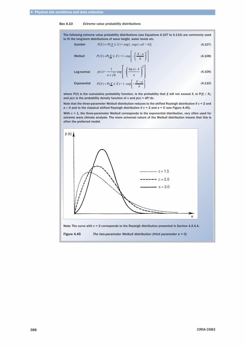
Box 4.10 Extreme value probability distributions
4 Physical site conditions and data collection
CIRIA C683388
The following extreme value probability distributions (see Equations 4.107 to 4.110) are commonly usedto fit the long-term distributions of wave height, water levels etc.
(4.107)
(4.108)
(4.109)
(4.110)
where P(X) is the cumulative probability function, ie the probability that X will not exceed X, ie P(X ≤ X),and p(x) is the probability density function of x and p(x) = dP/dx.
Note that the three-parameter Weibull distribution reduces to the shifted Rayleigh distribution if c = 2 anda ≠ 0 and to the classical shifted Rayleigh distribution if c = 2 and a = 0 (see Figure 4.45).
With c = 1, the three-parameter Weibull corresponds to the exponential distribution, very often used forextreme wave climate analysis. The more universal nature of the Weibull distribution means that this isoften the preferred model.
Note: The curve with c = 2 corresponds to the Rayleigh distribution presented in Section 4.2.4.4.
Figure 4.45 The two-parameter Weibull distribution (third parameter a = 0)
Gumbel
Exponential
Log-normal
Weibull
P X X X aX + b( ) P= ≤( ) = exp [ - exp (- )]
p x = a x
- x - b
a( ) exp
ln( )12
π
⎛⎝⎜
⎞⎠⎟
⎡
⎣⎢⎢
⎤
⎦⎥⎥
P X X X X - ab
c
( ) = 1 - exp - = ≤ ⎛⎝⎜
⎞⎠⎟
⎡
⎣⎢⎢
⎤
⎦⎥⎥
P( )
P X X X = - X ab
( ) P( )= ≤ − −⎡⎣⎢
⎤⎦⎥
1 exp
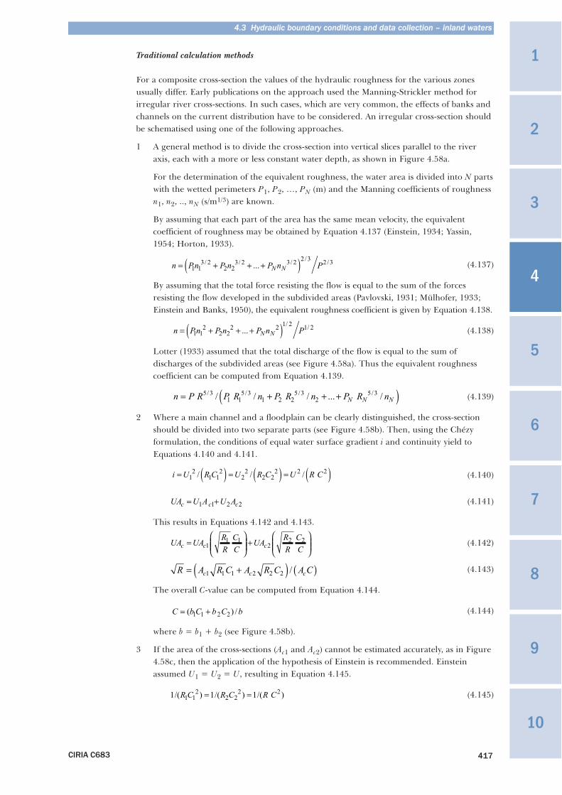
XXX
CIRIA C683 417
Traditional calculation methods
For a composite cross-section the values of the hydraulic roughness for the various zonesusually differ. Early publications on the approach used the Manning-Strickler method forirregular river cross-sections. In such cases, which are very common, the effects of banks andchannels on the current distribution have to be considered. An irregular cross-section shouldbe schematised using one of the following approaches.
1 A general method is to divide the cross-section into vertical slices parallel to the riveraxis, each with a more or less constant water depth, as shown in Figure 4.58a.
For the determination of the equivalent roughness, the water area is divided into N partswith the wetted perimeters P1, P2, …, PN (m) and the Manning coefficients of roughnessn1, n2, .., nN (s/m1/3) are known.
By assuming that each part of the area has the same mean velocity, the equivalentcoefficient of roughness may be obtained by Equation 4.137 (Einstein, 1934; Yassin,1954; Horton, 1933).
(4.137)
By assuming that the total force resisting the flow is equal to the sum of the forcesresisting the flow developed in the subdivided areas (Pavlovski, 1931; Mülhofer, 1933;Einstein and Banks, 1950), the equivalent roughness coefficient is given by Equation 4.138.
(4.138)
Lotter (1933) assumed that the total discharge of the flow is equal to the sum ofdischarges of the subdivided areas (see Figure 4.58a). Thus the equivalent roughnesscoefficient can be computed from Equation 4.139.
(4.139)
2 Where a main channel and a floodplain can be clearly distinguished, the cross-sectionshould be divided into two separate parts (see Figure 4.58b). Then, using the Chézyformulation, the conditions of equal water surface gradient i and continuity yield toEquations 4.140 and 4.141.
(4.140)
(4.141)
This results in Equations 4.142 and 4.143.
(4.142)
(4.143)
The overall C-value can be computed from Equation 4.144.
(4.144)
where b = b1 + b2 (see Figure 4.58b).
3 If the area of the cross-sections (Ac1 and Ac2) cannot be estimated accurately, as in Figure4.58c, then the application of the hypothesis of Einstein is recommended. Einsteinassumed U1 = U2 = U, resulting in Equation 4.145.
(4.145)
4.3 Hydraulic boundary conditions and data collection – inland waters
n Pn P n P n PN N= + + +( )1 12
2 22 2
1 21 2...
//
n P R P R n P R n P R nN N N= + + +( )5 31 1
5 31 2 2
5 32
5 3/ / / // / / ... /
i U R C U R C U R C= ( ) = ( ) = ( )12
1 12
22
2 22 2 2/ / /
n Pn P n P n PN N= + + +( )1 13 2
2 23 2 3 2
2 32 3/ / /
//...
UA U A U Ac c c= +1 1 2 2
UA UA RR
CC
UA RR
CCc c c=
⎛
⎝⎜⎜
⎞
⎠⎟⎟ +
⎛
⎝⎜⎜
⎞
⎠⎟⎟1
1 12
2 2
R A R C A R C A Cc c c= +( ) ( )1 1 1 2 2 2 /
C b C b C b= +( ) /1 1 2 2
1 1 11 12
2 22 2/( ) /( ) /( )R C R C R C= =
1
3
4
10
9
8
7
6
5
2
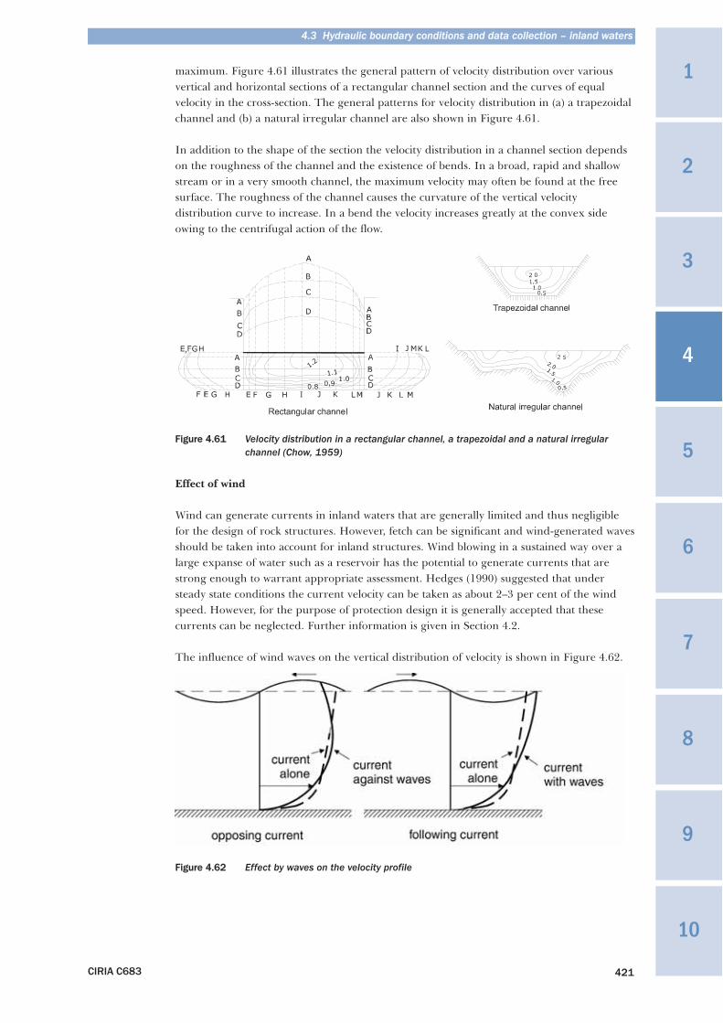
maximum. Figure 4.61 illustrates the general pattern of velocity distribution over variousvertical and horizontal sections of a rectangular channel section and the curves of equalvelocity in the cross-section. The general patterns for velocity distribution in (a) a trapezoidalchannel and (b) a natural irregular channel are also shown in Figure 4.61.
In addition to the shape of the section the velocity distribution in a channel section dependson the roughness of the channel and the existence of bends. In a broad, rapid and shallowstream or in a very smooth channel, the maximum velocity may often be found at the freesurface. The roughness of the channel causes the curvature of the vertical velocitydistribution curve to increase. In a bend the velocity increases greatly at the convex sideowing to the centrifugal action of the flow.
Figure 4.61 Velocity distribution in a rectangular channel, a trapezoidal and a natural irregular channel (Chow, 1959)
Effect of wind
Wind can generate currents in inland waters that are generally limited and thus negligiblefor the design of rock structures. However, fetch can be significant and wind-generated wavesshould be taken into account for inland structures. Wind blowing in a sustained way over alarge expanse of water such as a reservoir has the potential to generate currents that arestrong enough to warrant appropriate assessment. Hedges (1990) suggested that understeady state conditions the current velocity can be taken as about 2–3 per cent of the windspeed. However, for the purpose of protection design it is generally accepted that thesecurrents can be neglected. Further information is given in Section 4.2.
The influence of wind waves on the vertical distribution of velocity is shown in Figure 4.62.
Figure 4.62 Effect by waves on the velocity profile
4.3 Hydraulic boundary conditions and data collection – inland waters
CIRIA C683 421
1
3
4
10
9
8
7
6
5
2
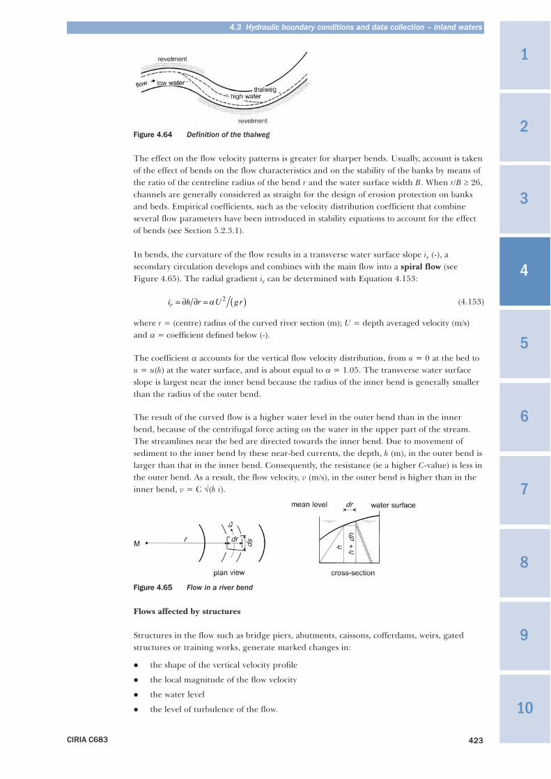
CIRIA C683 423
Figure 4.64 Definition of the thalweg
The effect on the flow velocity patterns is greater for sharper bends. Usually, account is takenof the effect of bends on the flow characteristics and on the stability of the banks by means ofthe ratio of the centreline radius of the bend r and the water surface width B. When r/B ≥ 26,channels are generally considered as straight for the design of erosion protection on banksand beds. Empirical coefficients, such as the velocity distribution coefficient that combineseveral flow parameters have been introduced in stability equations to account for the effectof bends (see Section 5.2.3.1).
In bends, the curvature of the flow results in a transverse water surface slope ir (-), asecondary circulation develops and combines with the main flow into a spiral flow (seeFigure 4.65). The radial gradient ir can be determined with Equation 4.153:
(4.153)
where r = (centre) radius of the curved river section (m); U = depth averaged velocity (m/s)and α = coefficient defined below (-).
The coefficient α accounts for the vertical flow velocity distribution, from u = 0 at the bed tou = u(h) at the water surface, and is about equal to α = 1.05. The transverse water surfaceslope is largest near the inner bend because the radius of the inner bend is generally smallerthan the radius of the outer bend.
The result of the curved flow is a higher water level in the outer bend than in the innerbend, because of the centrifugal force acting on the water in the upper part of the stream.The streamlines near the bed are directed towards the inner bend. Due to movement ofsediment to the inner bend by these near-bed currents, the depth, h (m), in the outer bend islarger than that in the inner bend. Consequently, the resistance (ie a higher C-value) is less inthe outer bend. As a result, the flow velocity, v (m/s), in the outer bend is higher than in theinner bend, v = C √(h i).
Figure 4.65 Flow in a river bend
Flows affected by structures
Structures in the flow such as bridge piers, abutments, caissons, cofferdams, weirs, gatedstructures or training works, generate marked changes in:
� the shape of the vertical velocity profile
� the local magnitude of the flow velocity
� the water level
� the level of turbulence of the flow.
4.3 Hydraulic boundary conditions and data collection – inland waters
i h r U g rr = ∂ ∂ = ( )α 2
1
3
4
10
9
8
7
6
5
2
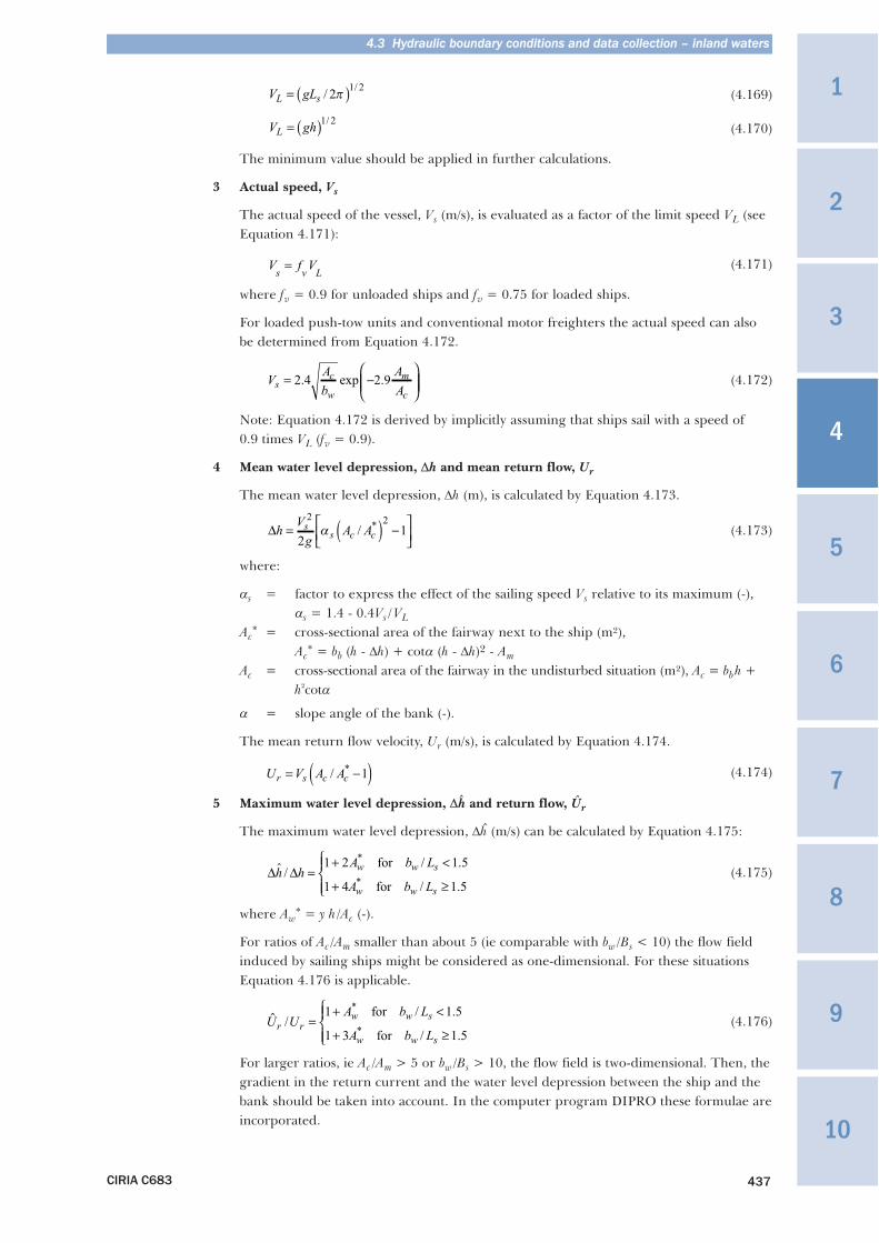
(4.169)
(4.170)
The minimum value should be applied in further calculations.
3 Actual speed, Vs
The actual speed of the vessel, Vs (m/s), is evaluated as a factor of the limit speed VL (seeEquation 4.171):
(4.171)
where fv = 0.9 for unloaded ships and fv = 0.75 for loaded ships.
For loaded push-tow units and conventional motor freighters the actual speed can alsobe determined from Equation 4.172.
(4.172)
Note: Equation 4.172 is derived by implicitly assuming that ships sail with a speed of0.9 times VL (fv = 0.9).
4 Mean water level depression, Δh and mean return flow, Ur
The mean water level depression, Δh (m), is calculated by Equation 4.173.
(4.173)
where:
αs = factor to express the effect of the sailing speed Vs relative to its maximum (-),αs = 1.4 - 0.4Vs /VL
Ac* = cross-sectional area of the fairway next to the ship (m²),
Ac* = bb (h - Δh) + cotα (h - Δh)2 - Am
Ac = cross-sectional area of the fairway in the undisturbed situation (m²), Ac = bbh +h²cotα
α = slope angle of the bank (-).
The mean return flow velocity, Ur (m/s), is calculated by Equation 4.174.
(4.174)
5 Maximum water level depression, Δh and return flow, Ûr
The maximum water level depression, Δh (m/s) can be calculated by Equation 4.175:
(4.175)
where Aw* = y h /Ac (-).
For ratios of Ac /Am smaller than about 5 (ie comparable with bw /Bs < 10) the flow fieldinduced by sailing ships might be considered as one-dimensional. For these situationsEquation 4.176 is applicable.
(4.176)
For larger ratios, ie Ac /Am > 5 or bw /Bs > 10, the flow field is two-dimensional. Then, thegradient in the return current and the water level depression between the ship and thebank should be taken into account. In the computer program DIPRO these formulae areincorporated.
4.3 Hydraulic boundary conditions and data collection – inland waters
CIRIA C683 437
V gLL s= ( )//
21 2π
V ghL = ( )1 2/
V f Vs v L=
V Ab
AAs
c
w
m
c= −
⎛
⎝⎜⎜
⎞
⎠⎟⎟2 4 2 9. exp .
Δh Vg
A Ass c c= ( ) −⎡
⎣⎢⎤⎦⎥
2 2
21α / *
U V A Ar s c c= −( )/ * 1
Δ Δh hA b L
A b Lw w s
w w s
// .
/ .
*
*=
+ <
+ ≥
⎧⎨⎪
⎩⎪
1 2 1 5
1 5
for
1 4 for
U UA b L
A b Lr r
w w s
w w s
// .
/ .
*
*=
+ <
+ ≥
⎧⎨⎪
⎩⎪
1 1 5
1 5
for
1 3 for
ˆ
ˆ
ˆ
ˆ
1
3
4
10
9
8
7
6
5
2
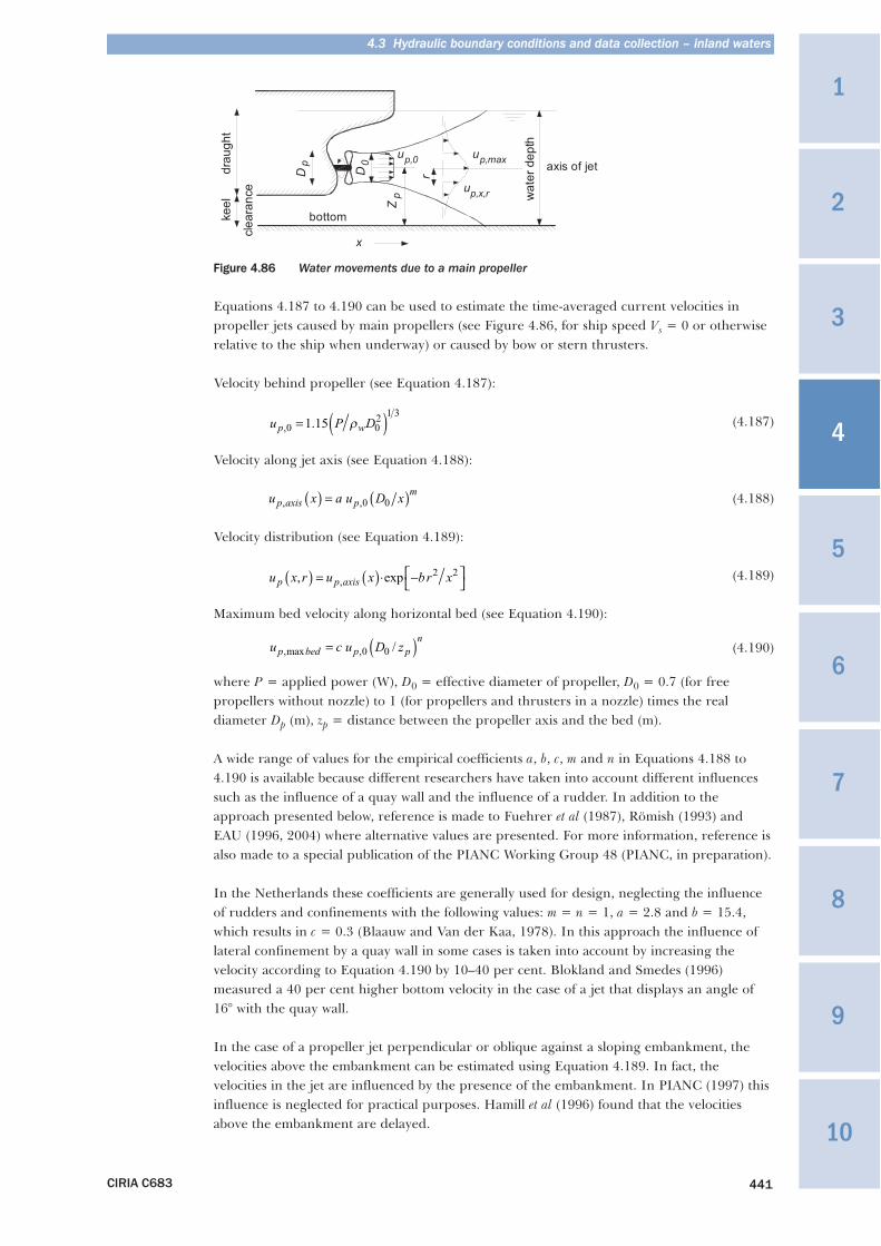
XXX
CIRIA C683 441
Figure 4.86 Water movements due to a main propeller
Equations 4.187 to 4.190 can be used to estimate the time-averaged current velocities inpropeller jets caused by main propellers (see Figure 4.86, for ship speed Vs = 0 or otherwiserelative to the ship when underway) or caused by bow or stern thrusters.
Velocity behind propeller (see Equation 4.187):
(4.187)
Velocity along jet axis (see Equation 4.188):
(4.188)
Velocity distribution (see Equation 4.189):
(4.189)
Maximum bed velocity along horizontal bed (see Equation 4.190):
(4.190)
where P = applied power (W), D0 = effective diameter of propeller, D0 = 0.7 (for freepropellers without nozzle) to 1 (for propellers and thrusters in a nozzle) times the realdiameter Dp (m), zp = distance between the propeller axis and the bed (m).
A wide range of values for the empirical coefficients a, b, c, m and n in Equations 4.188 to4.190 is available because different researchers have taken into account different influencessuch as the influence of a quay wall and the influence of a rudder. In addition to theapproach presented below, reference is made to Fuehrer et al (1987), Römish (1993) andEAU (1996, 2004) where alternative values are presented. For more information, reference isalso made to a special publication of the PIANC Working Group 48 (PIANC, in preparation).
In the Netherlands these coefficients are generally used for design, neglecting the influenceof rudders and confinements with the following values: m = n = 1, a = 2.8 and b = 15.4,which results in c = 0.3 (Blaauw and Van der Kaa, 1978). In this approach the influence oflateral confinement by a quay wall in some cases is taken into account by increasing thevelocity according to Equation 4.190 by 10–40 per cent. Blokland and Smedes (1996)measured a 40 per cent higher bottom velocity in the case of a jet that displays an angle of16° with the quay wall.
In the case of a propeller jet perpendicular or oblique against a sloping embankment, thevelocities above the embankment can be estimated using Equation 4.189. In fact, thevelocities in the jet are influenced by the presence of the embankment. In PIANC (1997) thisinfluence is neglected for practical purposes. Hamill et al (1996) found that the velocitiesabove the embankment are delayed.
4.3 Hydraulic boundary conditions and data collection – inland waters
bottom
clea
ranc
e
keel
Dp
r
x
D
Zp p,x,ru
wat
er d
epth
axis of jet0
up,0 up,max
drau
ght
u P Dp w, .0 02
1 31 15= ( )ρ
u x a u D xp axis pm
, ,( ) = ( )0 0
u x r u x br xp p axis, exp,( ) = ( )⋅ −⎡⎣
⎤⎦
2 2
u c u D zp bed p pn
,max , /= ( )0 0
1
3
4
10
9
8
7
6
5
2
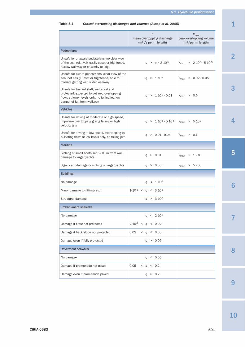
Table 5.4 Critical overtopping discharges and volumes (Allsop et al, 2005)
5.1 Hydraulic performance
CIRIA C683 501
qmean overtopping discharge
(m³ /s per m length)
Vmaxpeak overtopping volume
(m³/per m length)
Pedestrians
Unsafe for unaware pedestrians, no clear viewof the sea, relatively easily upset or frightened,narrow walkway or proximity to edge
q > q > 3⋅10-5 Vmax > 2⋅10-3 - 5⋅10-3
Unsafe for aware pedestrians, clear view of thesea, not easily upset or frightened, able totolerate getting wet, wider walkway
q > 1⋅10-4 Vmax > 0.02 - 0.05
Unsafe for trained staff, well shod andprotected, expected to get wet, overtoppingflows at lower levels only, no falling jet, lowdanger of fall from walkway
q > 1⋅10-3 - 0.01 Vmax > 0.5
Vehicles
Unsafe for driving at moderate or high speed,impulsive overtopping giving falling or highvelocity jets
q > 1.10-5 - 5.10-5 Vmax > 5⋅10-3
Unsafe for driving at low speed, overtopping bypulsating flows at low levels only, no falling jets
q > 0.01 - 0.05 Vmax > 0.1
Marinas
Sinking of small boats set 5–10 m from wall,damage to larger yachts
q > 0.01 Vmax > 1 - 10
Significant damage or sinking of larger yachts q > 0.05 Vmax > 5 - 50
Buildings
No damage q < 1⋅10-6
Minor damage to fittings etc 1⋅10-6 < q < 3⋅10-5
Structural damage q > 3⋅10-5
Embankment seawalls
No damage q < 2⋅10-3
Damage if crest not protected 2⋅10-3 < q < 0.02
Damage if back slope not protected 0.02 < q < 0.05
Damage even if fully protected q > 0.05
Revetment seawalls
No damage q < 0.05
Damage if promenade not paved 0.05 < q < 0.2
Damage even if promenade paved q > 0.2
1
3
4
10
9
8
7
6
5
2
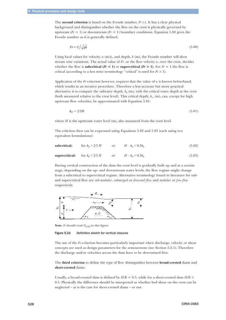
The second criterion is based on the Froude number, Fr (-). It has a clear physicalbackground and distinguishes whether the flow on the crest is physically governed byupstream (Fr > 1) or downstream (Fr < 1) boundary conditions. Equation 5.80 gives theFroude number as it is generally defined.
(5.80)
Using local values for velocity, u (m/s), and depth, h (m), the Froude number will showstream wise variations. The actual value of Fr, or the flow velocity u, over the crest, decideswhether the flow is subcritical (Fr < 1) or supercritical (Fr > 1). For Fr = 1 the flow iscritical (according to a less strict terminology “critical” is used for Fr ≥ 1).
Application of the Fr-criterion however, requires that the value of u is known beforehand,which results in an iterative procedure. Therefore a less accurate but more practicalalternative is to compare the tailwater depth, hb (m), with the critical water depth at the crest(both measured relative to the crest level). This critical depth, hcr (m), can, except for highupstream flow velocities, be approximated with Equation 5.81:
(5.81)
where H is the upstream water level (m), also measured from the crest level.
The criterion then can be expressed using Equations 5.82 and 5.83 (each using twoequivalent formulations):
subcritical: for hb > 2/3 H or H – hb < 0.5hb (5.82)
supercritical: for hb < 2/3 H or H – hb > 0.5hb (5.83)
During vertical construction of the dam the crest level is gradually built up and at a certainstage, depending on the up- and downstream water levels, the flow regime might changefrom a subcritical to supercritical regime. Alternative terminology found in literature for sub-and supercritical flow are sub-modular, submerged or drowned flow and modular or free flowrespectively.
Note: D should read Dn50 in this figure
Figure 5.21 Definition sketch for vertical closures
The use of the Fr-criterion becomes particularly important when discharge, velocity or shearconcepts are used as design parameters for the armourstone (see Section 5.2.1). Thereforethe discharge and/or velocities across the dam have to be determined first.
The third criterion to define the type of flow distinguishes between broad-crested dams andshort-crested dams:
Usually, a broad-crested dam is defined by H/B < 0.5, while for a short-crested dam H/B >0.5. Physically the difference should be interpreted as whether bed shear on the crest can beneglected – as is the case for short-crested dams – or not.
5 Physical processes and design tools
CIRIA C683528
Fr = U gh
h = Hcr 2/3
5.2 Structural response to hydraulic loading
CIRIA C683 539
� The principles of the shear concept are discussed in Section 5.2.1.3, based on the well-known Shields shear-type stability parameter introduced in Section 5.2.1.2. Some specificapplications (eg Pilarczyk’s formula) are discussed in Section 5.2.3. The method ofcritical shear is also applicable to oscillatory flow (waves only), as well as to a combinationof currents and waves (see Section 5.2.1.3).
� The critical or permissible velocity method is discussed in Section 5.2.1.4, based on thewell-known Izbash velocity-type stability parameter introduced in Section 5.2.1.2. Somespecific applications are shown in Section 5.2.3.
� The use of the H/(ΔD) wave stability criterion is introduced in Section 5.2.1.5 anddiscussed for different applications in Section 5.2.2.
� The use of the H/(ΔD) parameter to define a stability criterion in terms of a headdifference or height of overtopping across dams is introduced in Section 5.2.1.6 anddiscussed in Section 5.2.3.
� In Section 5.2.1.7 the critical discharge method is introduced.
The relationships used to transfer some stability parameters into others are described inSection 5.2.1.8. Finally, Section 5.2.1.9 gives an overview of the general design formulae.
5.2.1.2 Governing parameters to evaluate stability
Some of the parameters used to evaluate the hydraulic stability of rock structures consist ofcombinations of hydraulic (loading) parameters and material (resistance) parameters. Theparameters that are relevant for the structural stability, can be divided into four categories,discussed below:
� wave and current attack
� characterisation of armourstone
� cross-section of the structure
� response of the structure.
Wave attack
In the case of wave attack on a sloping structure the most important parameter, which gives arelationship (see Equation 5.95) between the structure and the wave conditions, is thestability number, Ns (-):
(5.95)
where:
H = wave height (m). This is usually the significant wave height, Hs, either definedby the average of the highest one third of the waves in a record, H1/3 , or by4√m0 , the spectral significant wave height Hm0 (see Section 4.2.4). For deepwater both definitions give more or less the same wave height. For shallow-water conditions there may be substantial differences up to H1/3 = 1.3 Hm0(see Section 4.2.4)
Δ = relative buoyant density (-), described by Equation 5.96 (see also Section 3.3.3.2)
D = characteristic size or diameter (m), depending on the type of structure (seeSection 5.2.2.1). The diameter used for armourstone is the median nominaldiameter, Dn50 (m), defined as the median equivalent cube size (see Section3.4.2). For concrete armour units the diameter used is Dn (m), which dependson the block shape (see Section 3.12).
N HD
s =Δ
1
3
4
10
9
8
7
6
5
2
5.2 Structural response to hydraulic loading
CIRIA C683 543
V = volume of the (concrete) armour unit (m³)
Dn = nominal diameter of the armour unit (m), Dn = (ks)1/3D, where ks is shapecoefficient and D is characteristic dimension of the concrete armour unit, ieblock height (see Section 3.12 for data).
The permeability of the structure is not defined in the standard way, as using Darcy’s law (seeSection 5.4.4.4), but is rather given as a notional index that represents the globalpermeability of the structure, or as a ratio of stone sizes. It is an important parameter withrespect to the stability of armour layers under wave attack. The permeability depends on thesize of the filter layers and core and can for example be given by a notional permeability factor,P. Examples of P are shown in Figure 5.39 in Section 5.2.2.2, based on the work of Van derMeer (1988b). A simpler approach to account for the influence of the permeability on thestability of rock-armoured slopes under wave or current attack uses the ratio of diameters ofcore material and armour material.
A practical measure for the permeability of dams (referring to the structure rather than thematerials) under current attack is the ratio between armourstone size, Dn50 (m), and damheight, d (m). This ratio, Dn50/d (-), sometimes also called “dam porosity”, may be interpretedas a measure for the voids in the rockfill.
The packing density is a parameter directly related to the placement pattern of the armourlayer. It is a term mainly applied to blocks in armour layers; the influence of the placementpattern on the stability of the structure is discussed in Section 5.2.2.3. Equation 5.99 gives theexpression for the estimate of the number of armour units per unit area, N (1/m²), as used inSections 3.5.1 and 3.12.
(5.99)
where:
N = Na/A (1/m²), where Na is the number of armour units in the area concerned (-);A is the surface area of the armour layer parallel to the local slope (m²); N issometimes called packing density
ta = armour layer thickness (m), defined by ta = nktDn50 (see also Section 3.5)
V = armour unit volume (m³).
NOTE: The packing density of concrete armour layers is the same as defined above inEquation 5.99, but then with Dn instead of Dn50. The packing density is then N = φ/Dn²,where φ is the packing density coefficient (-), see also Section 3.12.
The term packing density is rather widely used in literature, denoted as φ, when actually thepacking density coefficient, defined in Equation 5.99, is meant.
Parameters related to the response of the structure
The behaviour of the structure can be described by a number of parameters, depending on thetype of structure. Statically stable structures are described by the number of displaced units orby the development of damage, ie differences in the cross-section before and after storms.
The damage to the rock armour layer can be given as a percentage of displaced stonesrelated to a certain area, eg the entire layer or part of it. The damage percentage, D (%), hasoriginally been defined in the Shore protection manual (CERC, 1984) as:
The normalised eroded volume in the active zone, from the middle of the crest down to1Hs below still water level (SWL).
Nt n
Vnk n
Da v t v
n=
−( )=
−( )1 1
502
1
3
4
10
9
8
7
6
5
2
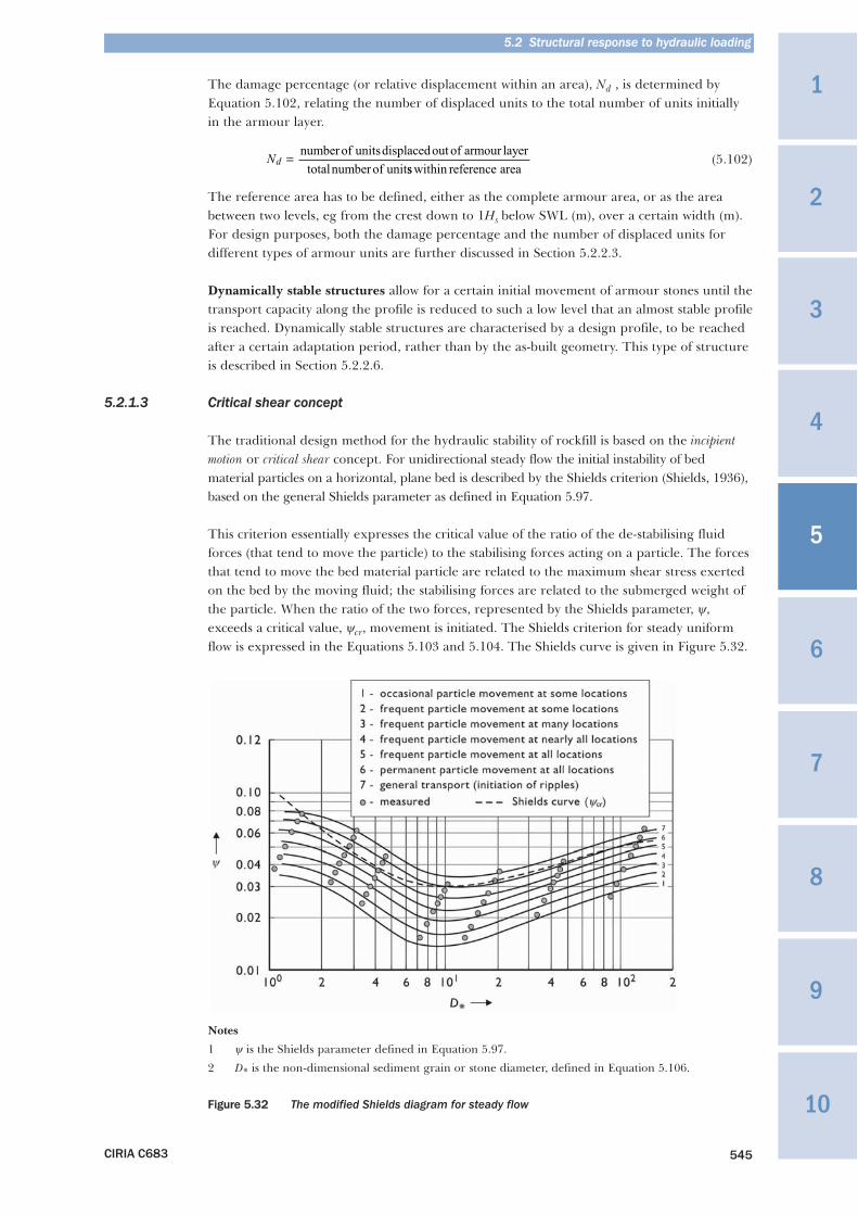
5.2 Structural response to hydraulic loading
CIRIA C683 545
The damage percentage (or relative displacement within an area), Nd , is determined byEquation 5.102, relating the number of displaced units to the total number of units initiallyin the armour layer.
(5.102)
The reference area has to be defined, either as the complete armour area, or as the areabetween two levels, eg from the crest down to 1Hs below SWL (m), over a certain width (m).For design purposes, both the damage percentage and the number of displaced units fordifferent types of armour units are further discussed in Section 5.2.2.3.
Dynamically stable structures allow for a certain initial movement of armour stones until thetransport capacity along the profile is reduced to such a low level that an almost stable profileis reached. Dynamically stable structures are characterised by a design profile, to be reachedafter a certain adaptation period, rather than by the as-built geometry. This type of structureis described in Section 5.2.2.6.
5.2.1.3 Critical shear concept
The traditional design method for the hydraulic stability of rockfill is based on the incipientmotion or critical shear concept. For unidirectional steady flow the initial instability of bedmaterial particles on a horizontal, plane bed is described by the Shields criterion (Shields, 1936),based on the general Shields parameter as defined in Equation 5.97.
This criterion essentially expresses the critical value of the ratio of the de-stabilising fluidforces (that tend to move the particle) to the stabilising forces acting on a particle. The forcesthat tend to move the bed material particle are related to the maximum shear stress exertedon the bed by the moving fluid; the stabilising forces are related to the submerged weight ofthe particle. When the ratio of the two forces, represented by the Shields parameter, ψ,exceeds a critical value, ψcr, movement is initiated. The Shields criterion for steady uniformflow is expressed in the Equations 5.103 and 5.104. The Shields curve is given in Figure 5.32.
Notes
1 ψ is the Shields parameter defined in Equation 5.97.
2 D* is the non-dimensional sediment grain or stone diameter, defined in Equation 5.106.
Figure 5.32 The modified Shields diagram for steady flow
Nd = number of unitsdisplacedout of armour layer
totalnumber of unitss within reference area
1
3
4
10
9
8
7
6
5
2
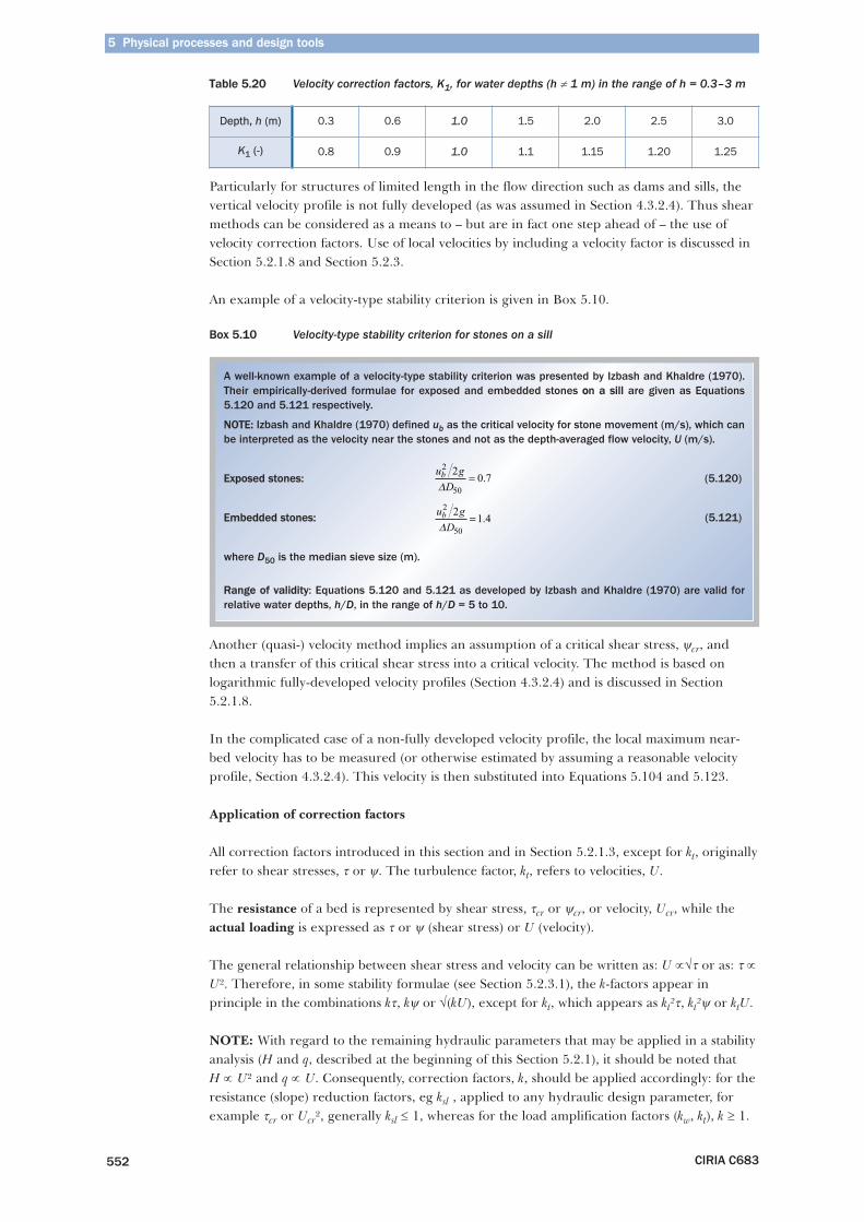
5 Physical processes and design tools
CIRIA C683552
Table 5.20 Velocity correction factors, K1, for water depths (h ≠ 1 m) in the range of h = 0.3–3 m
Particularly for structures of limited length in the flow direction such as dams and sills, thevertical velocity profile is not fully developed (as was assumed in Section 4.3.2.4). Thus shearmethods can be considered as a means to – but are in fact one step ahead of – the use ofvelocity correction factors. Use of local velocities by including a velocity factor is discussed inSection 5.2.1.8 and Section 5.2.3.
An example of a velocity-type stability criterion is given in Box 5.10.
Box 5.10 Velocity-type stability criterion for stones on a sill
Another (quasi-) velocity method implies an assumption of a critical shear stress, ψcr, andthen a transfer of this critical shear stress into a critical velocity. The method is based onlogarithmic fully-developed velocity profiles (Section 4.3.2.4) and is discussed in Section5.2.1.8.
In the complicated case of a non-fully developed velocity profile, the local maximum near-bed velocity has to be measured (or otherwise estimated by assuming a reasonable velocityprofile, Section 4.3.2.4). This velocity is then substituted into Equations 5.104 and 5.123.
Application of correction factors
All correction factors introduced in this section and in Section 5.2.1.3, except for kt, originallyrefer to shear stresses, τ or ψ. The turbulence factor, kt, refers to velocities, U.
The resistance of a bed is represented by shear stress, τcr or ψcr, or velocity, Ucr, while theactual loading is expressed as τ or ψ (shear stress) or U (velocity).
The general relationship between shear stress and velocity can be written as: U ∝√τ or as: τ ∝U². Therefore, in some stability formulae (see Section 5.2.3.1), the k-factors appear inprinciple in the combinations kτ, kψ or √(kU), except for kt, which appears as kt²τ, kt²ψ or ktU.
NOTE: With regard to the remaining hydraulic parameters that may be applied in a stabilityanalysis (H and q, described at the beginning of this Section 5.2.1), it should be noted that H ∝ U² and q ∝ U. Consequently, correction factors, k, should be applied accordingly: for theresistance (slope) reduction factors, eg ksl , applied to any hydraulic design parameter, forexample τcr or Ucr², generally ksl ≤ 1, whereas for the load amplification factors (kw, kt), k ≥ 1.
Depth, h (m) 0.3 0.6 1.0 1.5 2.0 2.5 3.0
K1 (-) 0.8 0.9 1.0 1.1 1.15 1.20 1.25
A well-known example of a velocity-type stability criterion was presented by Izbash and Khaldre (1970).Their empirically-derived formulae for exposed and embedded stones oon a sill are given as Equations5.120 and 5.121 respectively.
NOTE: Izbash and Khaldre (1970) defined ub as the critical velocity for stone movement (m/s), which canbe interpreted as the velocity near the stones and not as the depth-averaged flow velocity, U (m/s).
Exposed stones: (5.120)
Embedded stones: (5.121)
where D50 is the median sieve size (m).
Range of validity: Equations 5.120 and 5.121 as developed by Izbash and Khaldre (1970) are valid forrelative water depths, h/D, in the range of h/D = 5 to 10.
u gD
b2
50
21 4
Δ= .
u gD
b2
50
20 7
Δ= .
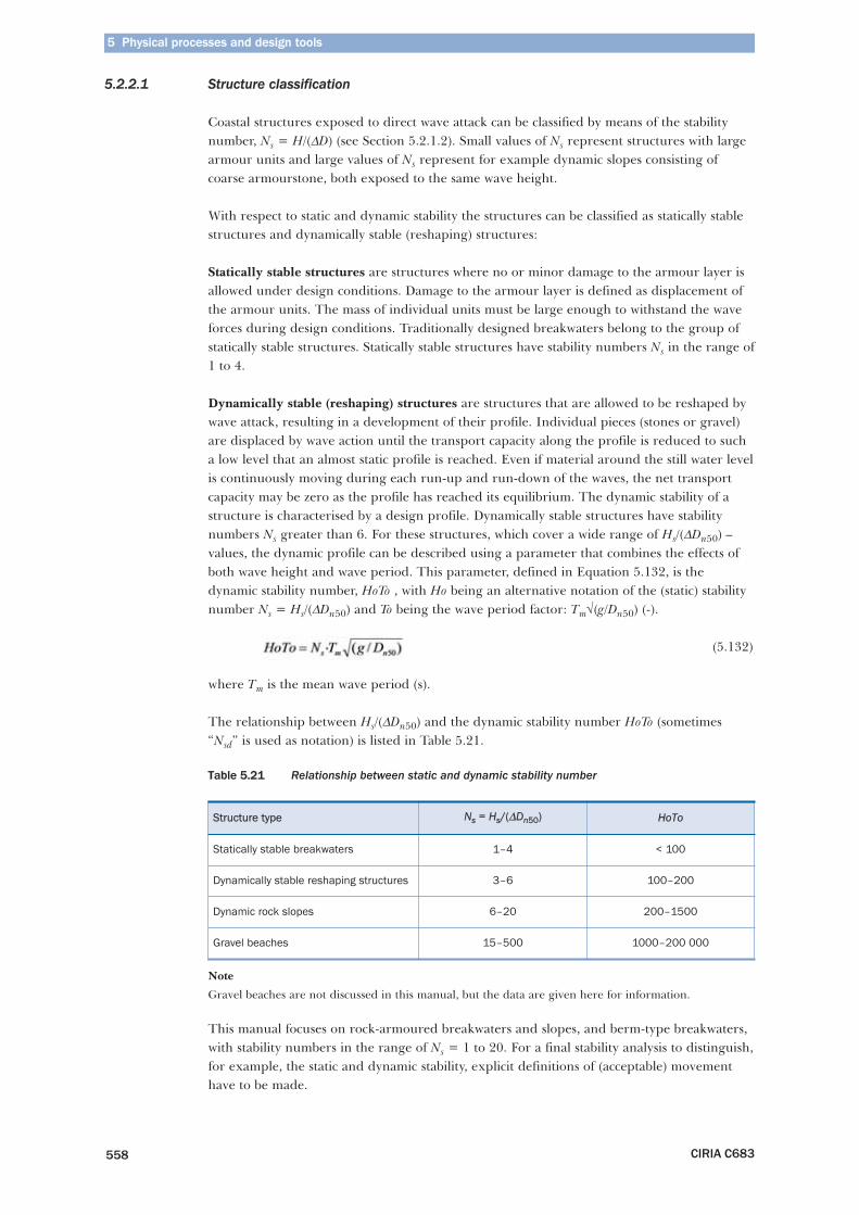
5 Physical processes and design tools
CIRIA C683558
5.2.2.1 Structure classification
Coastal structures exposed to direct wave attack can be classified by means of the stabilitynumber, Ns = H/(ΔD) (see Section 5.2.1.2). Small values of Ns represent structures with largearmour units and large values of Ns represent for example dynamic slopes consisting ofcoarse armourstone, both exposed to the same wave height.
With respect to static and dynamic stability the structures can be classified as statically stablestructures and dynamically stable (reshaping) structures:
Statically stable structures are structures where no or minor damage to the armour layer isallowed under design conditions. Damage to the armour layer is defined as displacement ofthe armour units. The mass of individual units must be large enough to withstand the waveforces during design conditions. Traditionally designed breakwaters belong to the group ofstatically stable structures. Statically stable structures have stability numbers Ns in the range of1 to 4.
Dynamically stable (reshaping) structures are structures that are allowed to be reshaped bywave attack, resulting in a development of their profile. Individual pieces (stones or gravel)are displaced by wave action until the transport capacity along the profile is reduced to sucha low level that an almost static profile is reached. Even if material around the still water levelis continuously moving during each run-up and run-down of the waves, the net transportcapacity may be zero as the profile has reached its equilibrium. The dynamic stability of astructure is characterised by a design profile. Dynamically stable structures have stabilitynumbers Ns greater than 6. For these structures, which cover a wide range of Hs/(ΔDn50) –values, the dynamic profile can be described using a parameter that combines the effects ofboth wave height and wave period. This parameter, defined in Equation 5.132, is thedynamic stability number, HoTo , with Ho being an alternative notation of the (static) stabilitynumber Ns = Hs/(ΔDn50) and To being the wave period factor: Tm√(g/Dn50) (-).
(5.132)
where Tm is the mean wave period (s).
The relationship between Hs/(ΔDn50) and the dynamic stability number HoTo (sometimes“Nsd” is used as notation) is listed in Table 5.21.
Table 5.21 Relationship between static and dynamic stability number
Note
Gravel beaches are not discussed in this manual, but the data are given here for information.
This manual focuses on rock-armoured breakwaters and slopes, and berm-type breakwaters,with stability numbers in the range of Ns = 1 to 20. For a final stability analysis to distinguish,for example, the static and dynamic stability, explicit definitions of (acceptable) movementhave to be made.
Structure type Ns = Hs/(ΔDn50) HoTo
Statically stable breakwaters 1–4 < 100
Dynamically stable reshaping structures 3–6 100–200
Dynamic rock slopes 6–20 200–1500
Gravel beaches 15–500 1000–200 000
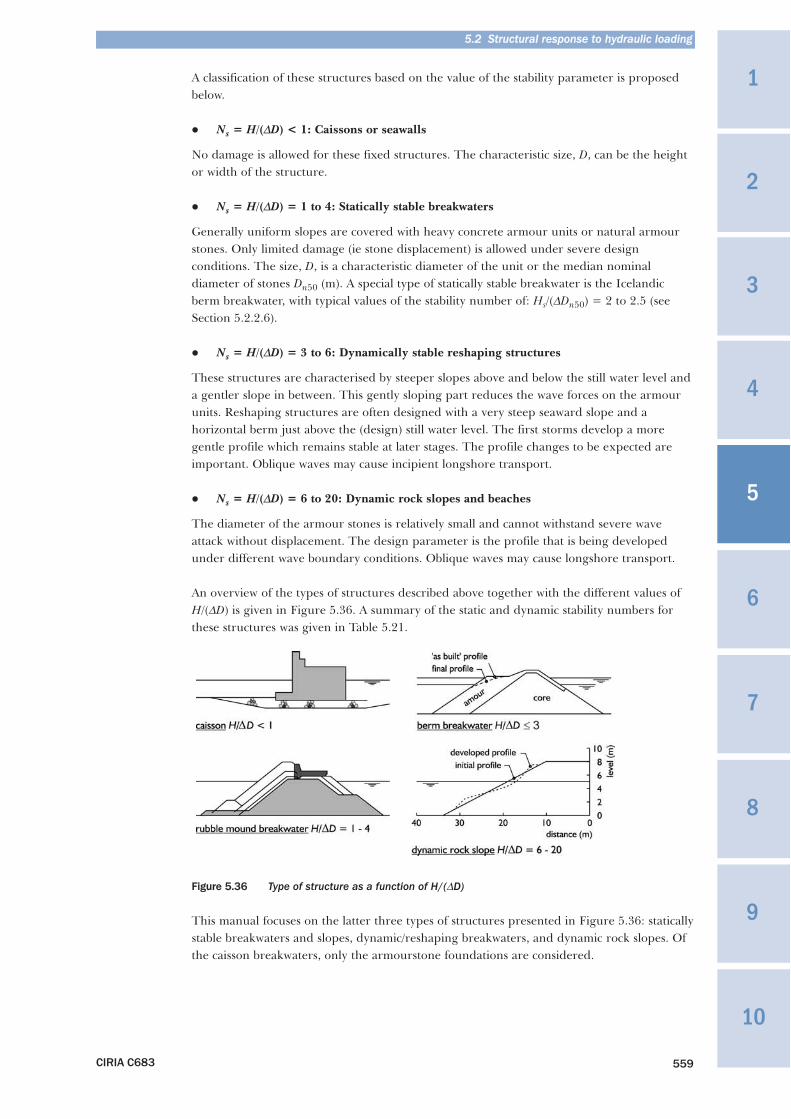
5.2 Structural response to hydraulic loading
CIRIA C683 559
A classification of these structures based on the value of the stability parameter is proposedbelow.
� Ns = H/(ΔD) < 1: Caissons or seawalls
No damage is allowed for these fixed structures. The characteristic size, D, can be the heightor width of the structure.
� Ns = H/(ΔD) = 1 to 4: Statically stable breakwaters
Generally uniform slopes are covered with heavy concrete armour units or natural armourstones. Only limited damage (ie stone displacement) is allowed under severe designconditions. The size, D, is a characteristic diameter of the unit or the median nominaldiameter of stones Dn50 (m). A special type of statically stable breakwater is the Icelandicberm breakwater, with typical values of the stability number of: Hs/(ΔDn50) = 2 to 2.5 (seeSection 5.2.2.6).
� Ns = H/(ΔD) = 3 to 6: Dynamically stable reshaping structures
These structures are characterised by steeper slopes above and below the still water level anda gentler slope in between. This gently sloping part reduces the wave forces on the armourunits. Reshaping structures are often designed with a very steep seaward slope and ahorizontal berm just above the (design) still water level. The first storms develop a moregentle profile which remains stable at later stages. The profile changes to be expected areimportant. Oblique waves may cause incipient longshore transport.
� Ns = H/(ΔD) = 6 to 20: Dynamic rock slopes and beaches
The diameter of the armour stones is relatively small and cannot withstand severe waveattack without displacement. The design parameter is the profile that is being developedunder different wave boundary conditions. Oblique waves may cause longshore transport.
An overview of the types of structures described above together with the different values ofH/(ΔD) is given in Figure 5.36. A summary of the static and dynamic stability numbers forthese structures was given in Table 5.21.
Figure 5.36 Type of structure as a function of H/(ΔD)
This manual focuses on the latter three types of structures presented in Figure 5.36: staticallystable breakwaters and slopes, dynamic/reshaping breakwaters, and dynamic rock slopes. Ofthe caisson breakwaters, only the armourstone foundations are considered.
1
3
4
10
9
8
7
6
5
2
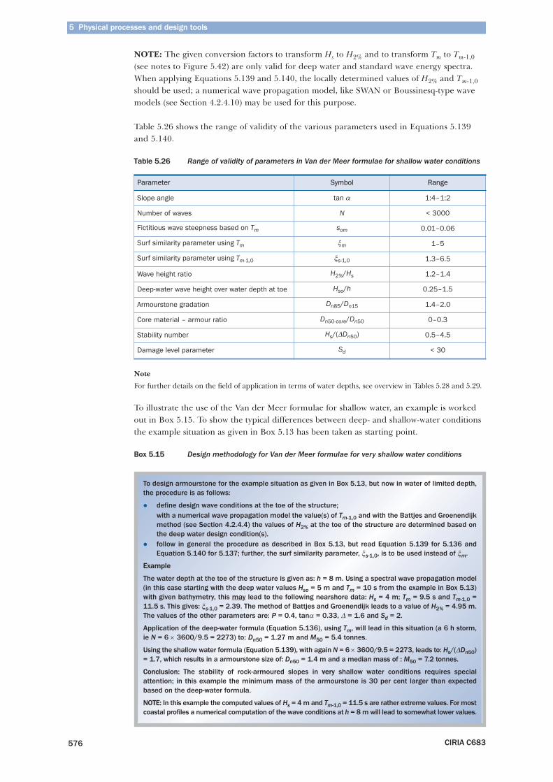
5 Physical processes and design tools
CIRIA C683576
NOTE: The given conversion factors to transform Hs to H2% and to transform Tm to Tm-1,0(see notes to Figure 5.42) are only valid for deep water and standard wave energy spectra.When applying Equations 5.139 and 5.140, the locally determined values of H2% and Tm-1,0should be used; a numerical wave propagation model, like SWAN or Boussinesq-type wavemodels (see Section 4.2.4.10) may be used for this purpose.
Table 5.26 shows the range of validity of the various parameters used in Equations 5.139and 5.140.
Table 5.26 Range of validity of parameters in Van der Meer formulae for shallow water conditions
Note
For further details on the field of application in terms of water depths, see overview in Tables 5.28 and 5.29.
To illustrate the use of the Van der Meer formulae for shallow water, an example is workedout in Box 5.15. To show the typical differences between deep- and shallow-water conditionsthe example situation as given in Box 5.13 has been taken as starting point.
Box 5.15 Design methodology for Van der Meer formulae for very shallow water conditions
Parameter Symbol Range
Slope angle tan α 1:4–1:2
Number of waves N < 3000
Fictitious wave steepness based on Tm som 0.01–0.06
Surf similarity parameter using Tm ξm 1–5
Surf similarity parameter using Tm-1,0 ξs-1,0 1.3–6.5
Wave height ratio H2%/Hs 1.2–1.4
Deep-water wave height over water depth at toe Hso/h 0.25–1.5
Armourstone gradation Dn85/Dn15 1.4–2.0
Core material – armour ratio Dn50-core/Dn50 0–0.3
Stability number Hs/(ΔDn50) 0.5–4.5
Damage level parameter Sd < 30
To design armourstone for the example situation as given in Box 5.13, but now in water of limited depth,the procedure is as follows:
� define design wave conditions at the toe of the structure;with a numerical wave propagation model the value(s) of Tm-1,0 and with the Battjes and Groenendijkmethod (see Section 4.2.4.4) the values of H2% at the toe of the structure are determined based onthe deep water design condition(s).
� follow in general the procedure as described in Box 5.13, but read Equation 5.139 for 5.136 andEquation 5.140 for 5.137; further, the surf similarity parameter, ξs-1,0, is to be used instead of ξm.
Example
The water depth at the toe of the structure is given as: h = 8 m. Using a spectral wave propagation model(in this case starting with the deep water values Hso = 5 m and Tm = 10 s from the example in Box 5.13)with given bathymetry, this may lead to the following nearshore data: Hs = 4 m; Tm = 9.5 s and Tm-1,0 =11.5 s. This gives: ξs-1,0 = 2.39. The method of Battjes and Groenendijk leads to a value of H2% = 4.95 m.The values of the other parameters are: P = 0.4, tanα = 0.33, Δ = 1.6 and Sd = 2.
Application of the deep-water formula (Equation 5.136), using Tm, will lead in this situation (a 6 h storm,ie N = 6 × 3600/9.5 = 2273) to: Dn50 = 1.27 m and M50 = 5.4 tonnes.
Using the shallow water formula (Equation 5.139), with again N = 6 × 3600/9.5 = 2273, leads to: Hs/(ΔDn50)= 1.7, which results in a armourstone size of: Dn50 = 1.4 m and a median mass of : M50 = 7.2 tonnes.
Conclusion: The stability of rock-armoured slopes in vvery shallow water conditions requires specialattention; in this example the minimum mass of the armourstone is 30 per cent larger than expectedbased on the deep-water formula.
NOTE: In this example the computed values of Hs = 4 m and Tm-1,0 = 11.5 s are rather extreme values. For mostcoastal profiles a numerical computation of the wave conditions at h = 8 m will lead to somewhat lower values.
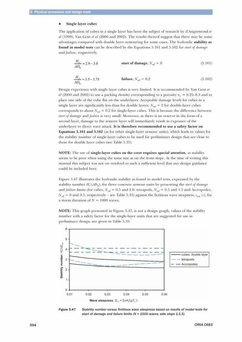
5 Physical processes and design tools
CIRIA C683594
� Single layer cubes
The application of cubes in a single layer has been the subject of research by d’Angremond etal (1999), Van Gent et al (2000 and 2002). The results thereof suggest that there may be someadvantages compared with double layer armouring for some cases. The hydraulic stability asfound in model tests can be described by the Equations 5.161 and 5.162 for start of damageand failure, respectively.
start of damage, Nod = 0 (5.161)
failure, Nod = 0.2 (5.162)
Design experience with single layer cubes is very limited. It is recommended by Van Gent etal (2000 and 2002) to use a packing density corresponding to a porosity nv = 0.25–0.3 and toplace one side of the cube flat on the underlayer. Acceptable damage levels for cubes in asingle layer are significantly less than for double layers: Nod = 2 for double-layer cubescorresponds to about Nod = 0.2 for single-layer cubes. This is because the difference betweenstart of damage and failure is very small. Moreover, as there is no reserve in the form of asecond layer, damage to the armour layer will immediately result in exposure of theunderlayer to direct wave attack. It is therefore recommended to use a safety factor onEquations 5.161 and 5.162 (as for other single-layer armour units), which leads to values forthe stability number of single-layer cubes to be used for preliminary design that are close tothose for double layer cubes (see Table 5.35).
NOTE: The use of single-layer cubes on the crest requires special attention, as stabilityseems to be poor when using the same size as on the front slope. At the time of writing thismanual this subject was not yet resolved to such a sufficient level that any design guidancecould be included here.
Figure 5.47 illustrates the hydraulic stability as found in model tests, expressed by thestability number Hs/(ΔDn), for three concrete armour units by presenting the start of damageand failure limits (for cubes, Nod = 0.5 and 2.0; tetrapods, Nod = 0.5 and 1.5 and Accropodes,Nod = 0 and 0.5, respectively – see Table 5.33) against the fictitious wave steepness, som (-), fora storm duration of N = 1000 waves.
NOTE: This graph presented in Figure 5.47, is not a design graph; values of the stabilitynumber with a safety factor for the single-layer units that are suggested for use inpreliminary design, are given in Table 5.35.
Figure 5.47 Stability number versus fictitious wave steepness based on results of model tests forstart of damage and failure limits (N = 1000 waves; side slope 1:1.5)
HD
s
nΔ= −2 9 3 0. .
HD
s
nΔ= −3 5 3 75. .
5 Physical processes and design tools
CIRIA C683600
The stability of the armourstone on the front slope of a low-crested emergent structure canbe related to the stability of a non-overtopped structure. This can be achieved by firstcalculating the required nominal diameter of the armour unit with one of the designformulae presented in Section 5.2.2.2 for rock armour layers and then applying a reductionfactor on this nominal diameter, Dn50. It is, however, advised to take great care whenreducing the armour size of a low-crested breakwater.
This approach has been adopted by Van der Meer (1990a). He suggested that thearmourstone cover layer stability formulae (Van der Meer, 1988b) (see Section 5.2.2.2) can beused with Dn50 replaced by rDDn50. The reduction factor, rD (-), on the stone size required, isgiven as Equation 5.164:
(5.164)
where Rc is the crest freeboard (m), and sop the fictitious wave steepness (-), based on thepeak wave period, Tp (s).
NOTE: The factor Rc/Hs·√(sop/2π) is equal to Owen’s dimensionless freeboard, R* (see Section5.1.1.3, Equation 5.28).
Design curves are given in Box 5.20. The limits of Equation 5.164 are given by Equation5.165 as:
(5.165)
NOTE: Equation 5.164 gives an estimate for the required stone diameter on the front slope.For the crest and the rear side a similar size of material or larger material may be required.
Rule of thumb for emergent structures
As a rule of thumb Equation 5.166 can be used to obtain a first estimate of the stone size,Dn50 (m), in a conceptual design phase for emergent structures (Kramer and Burcharth,2004) in depth-limited wave conditions, ie with breaking waves on the foreshore.
(5.166)
where Hs is the significant wave height at the toe of the structure (m); h is the water depth atthe toe of the structure (m); αs is the slope angle of the foreshore (°).
NOTE: Other values for Hs/h, cotαs and Δ might lead to very different values for the stonesize required.
r RH
sD
c
s
op= −⎛
⎝⎜⎜
⎞
⎠⎟⎟
−
1 25 4 82
1
. .π
02
0 052< <RH
sc
s
op
π.
D h Hhn
ss50 0 3 0 6 100≥ = ≥ ≅. . , cot for and 1.6α Δ
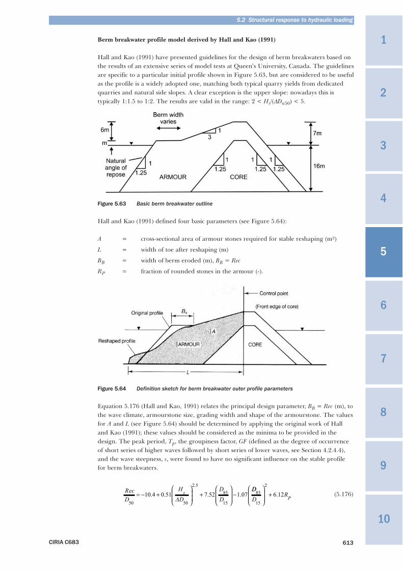
5.2 Structural response to hydraulic loading
CIRIA C683 613
1
3
4
10
9
8
7
6
5
2
Berm breakwater profile model derived by Hall and Kao (1991)
Hall and Kao (1991) have presented guidelines for the design of berm breakwaters based onthe results of an extensive series of model tests at Queen’s University, Canada. The guidelinesare specific to a particular initial profile shown in Figure 5.63, but are considered to be usefulas the profile is a widely adopted one, matching both typical quarry yields from dedicatedquarries and natural side slopes. A clear exception is the upper slope: nowadays this istypically 1:1.5 to 1:2. The results are valid in the range: 2 < Hs/(ΔDn50) < 5.
Figure 5.63 Basic berm breakwater outline
Hall and Kao (1991) defined four basic parameters (see Figure 5.64):
A = cross-sectional area of armour stones required for stable reshaping (m²)
L = width of toe after reshaping (m)
BB = width of berm eroded (m), BB = Rec
RP = fraction of rounded stones in the armour (-).
Figure 5.64 Definition sketch for berm breakwater outer profile parameters
Equation 5.176 (Hall and Kao, 1991) relates the principal design parameter, BB = Rec (m), tothe wave climate, armourstone size, grading width and shape of the armourstone. The valuesfor A and L (see Figure 5.64) should be determined by applying the original work of Halland Kao (1991); these values should be considered as the minima to be provided in thedesign. The peak period, Tp, the groupiness factor, GF (defined as the degree of occurrenceof short series of higher waves followed by short series of lower waves, see Section 4.2.4.4),and the wave steepness, s, were found to have no significant influence on the stable profilefor berm breakwaters.
(5.176)RecD
H
D
D
Ds
50 50
2 5
85
15
10 4 0 51 7 52 1 07= − +⎛
⎝⎜⎜
⎞
⎠⎟⎟
+⎛
⎝⎜⎜
⎞
⎠⎟⎟
−. . . .
.
Δ
DD
DRP
85
15
2
6 12⎛
⎝⎜⎜
⎞
⎠⎟⎟
+ .
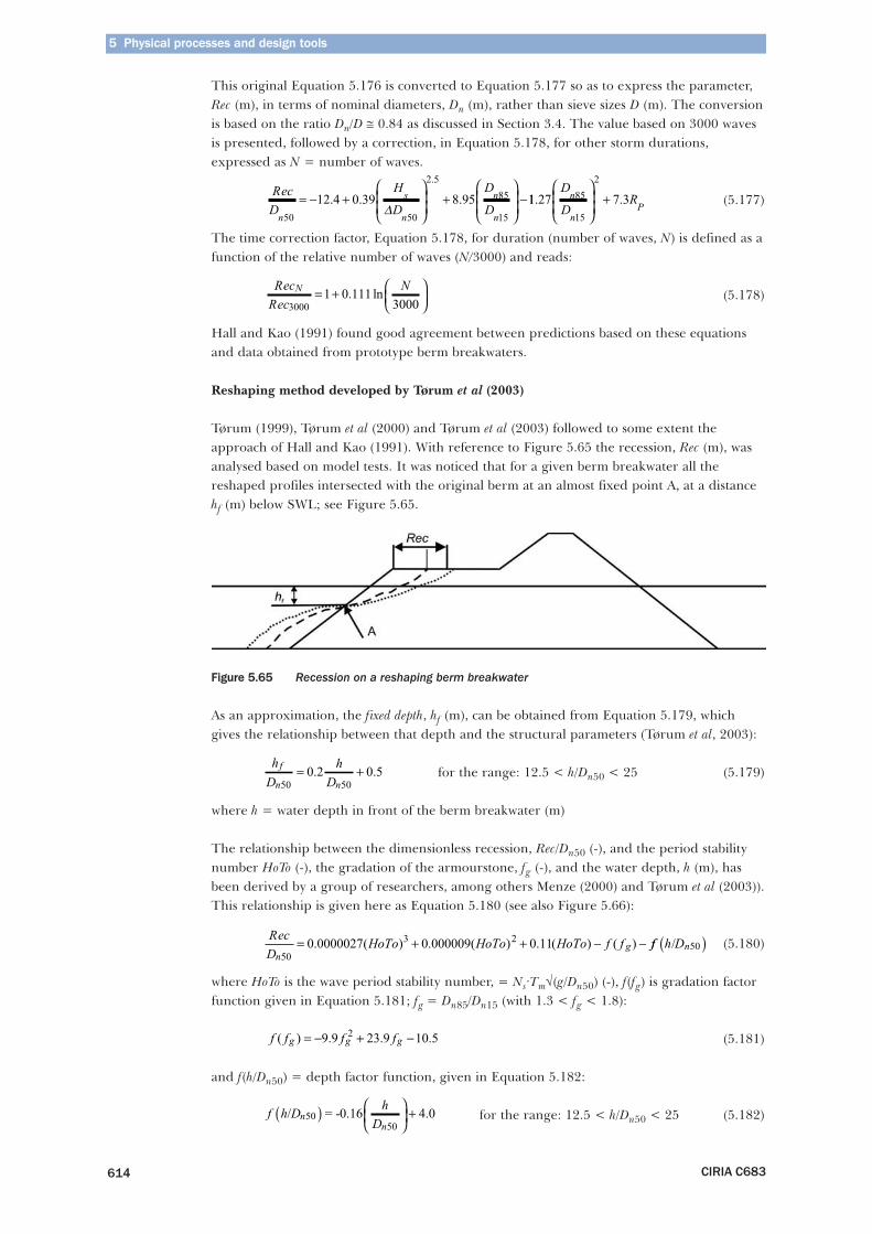
5 Physical processes and design tools
CIRIA C683614
This original Equation 5.176 is converted to Equation 5.177 so as to express the parameter,Rec (m), in terms of nominal diameters, Dn (m), rather than sieve sizes D (m). The conversionis based on the ratio Dn/D ≅ 0.84 as discussed in Section 3.4. The value based on 3000 wavesis presented, followed by a correction, in Equation 5.178, for other storm durations,expressed as N = number of waves.
(5.177)
The time correction factor, Equation 5.178, for duration (number of waves, N) is defined as afunction of the relative number of waves (N/3000) and reads:
(5.178)
Hall and Kao (1991) found good agreement between predictions based on these equationsand data obtained from prototype berm breakwaters.
Reshaping method developed by Tørum et al (2003)
Tørum (1999), Tørum et al (2000) and Tørum et al (2003) followed to some extent theapproach of Hall and Kao (1991). With reference to Figure 5.65 the recession, Rec (m), wasanalysed based on model tests. It was noticed that for a given berm breakwater all thereshaped profiles intersected with the original berm at an almost fixed point A, at a distancehf (m) below SWL; see Figure 5.65.
Figure 5.65 Recession on a reshaping berm breakwater
As an approximation, the fixed depth, hf (m), can be obtained from Equation 5.179, whichgives the relationship between that depth and the structural parameters (Tørum et al, 2003):
for the range: 12.5 < h/Dn50 < 25 (5.179)
where h = water depth in front of the berm breakwater (m)
The relationship between the dimensionless recession, Rec/Dn50 (-), and the period stabilitynumber HoTo (-), the gradation of the armourstone, fg (-), and the water depth, h (m), hasbeen derived by a group of researchers, among others Menze (2000) and Tørum et al (2003)).This relationship is given here as Equation 5.180 (see also Figure 5.66):
(5.180)
where HoTo is the wave period stability number, = Ns·Tm√(g/Dn50) (-), f(fg) is gradation factorfunction given in Equation 5.181; fg = Dn85/Dn15 (with 1.3 < fg < 1.8):
(5.181)
and f(h/Dn50) = depth factor function, given in Equation 5.182:
for the range: 12.5 < h/Dn50 < 25 (5.182)
RecD
H
D
D
Dn
s
n
n
n50 50
2 5
85
15
12 4 0 39 8 95= − +⎛
⎝⎜⎜
⎞
⎠⎟⎟
+⎛
⎝⎜⎜
⎞
⎠⎟⎟
−. . .
.
Δ11 27 7 385
15
2
. .D
DRn
nP
⎛
⎝⎜⎜
⎞
⎠⎟⎟
+
RecRec
NN
3000
1 0 1113000
= + ⎛⎝⎜
⎞⎠⎟
. ln
hD
hD
f
n n50 50
0 2 0 5= +. .
f hDn
h Dn/ = -0.1650( ) ⎛⎝⎜
⎞⎠⎟ +
50
4 0.
f f f fg g g( ) . . .= − + −9 9 23 9 10 52
RecD
HoTo HoTo HoTo f fn
g50
3 20 0000027 0 000009 0 11= + + − −. ( ) . ( ) . ( ) ( ) ff h Dn/ 50( )
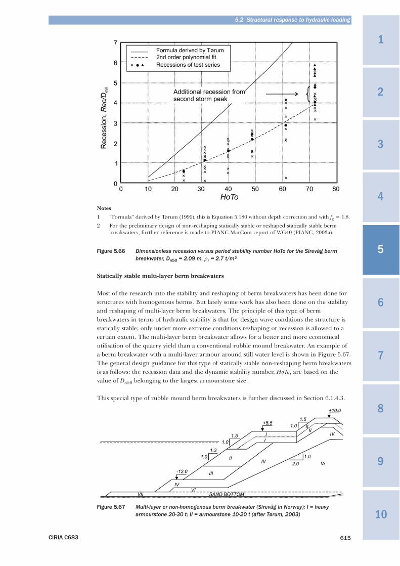
5.2 Structural response to hydraulic loading
CIRIA C683 615
1
3
4
10
9
8
7
6
5
2
Notes
1 “Formula” derived by Tørum (1999), this is Equation 5.180 without depth correction and with fg = 1.8.
2 For the preliminary design of non-reshaping statically stable or reshaped statically stable bermbreakwaters, further reference is made to PIANC MarCom report of WG40 (PIANC, 2003a).
Figure 5.66 Dimensionless recession versus period stability number HoTo for the Sirevåg bermbreakwater, Dn50 = 2.09 m, ρr = 2.7 t/m²
Statically stable multi-layer berm breakwaters
Most of the research into the stability and reshaping of berm breakwaters has been done forstructures with homogenous berms. But lately some work has also been done on the stabilityand reshaping of multi-layer berm breakwaters. The principle of this type of bermbreakwaters in terms of hydraulic stability is that for design wave conditions the structure isstatically stable; only under more extreme conditions reshaping or recession is allowed to acertain extent. The multi-layer berm breakwater allows for a better and more economicalutilisation of the quarry yield than a conventional rubble mound breakwater. An example ofa berm breakwater with a multi-layer armour around still water level is shown in Figure 5.67.The general design guidance for this type of statically stable non-reshaping berm breakwatersis as follows: the recession data and the dynamic stability number, HoTo, are based on thevalue of Dn50 belonging to the largest armourstone size.
This special type of rubble mound berm breakwaters is further discussed in Section 6.1.4.3.
Figure 5.67 Multi-layer or non-homogenous berm breakwater (Sirevåg in Norway); I = heavyarmourstone 20-30 t; II = armourstone 10-20 t (after Tørum, 2003)
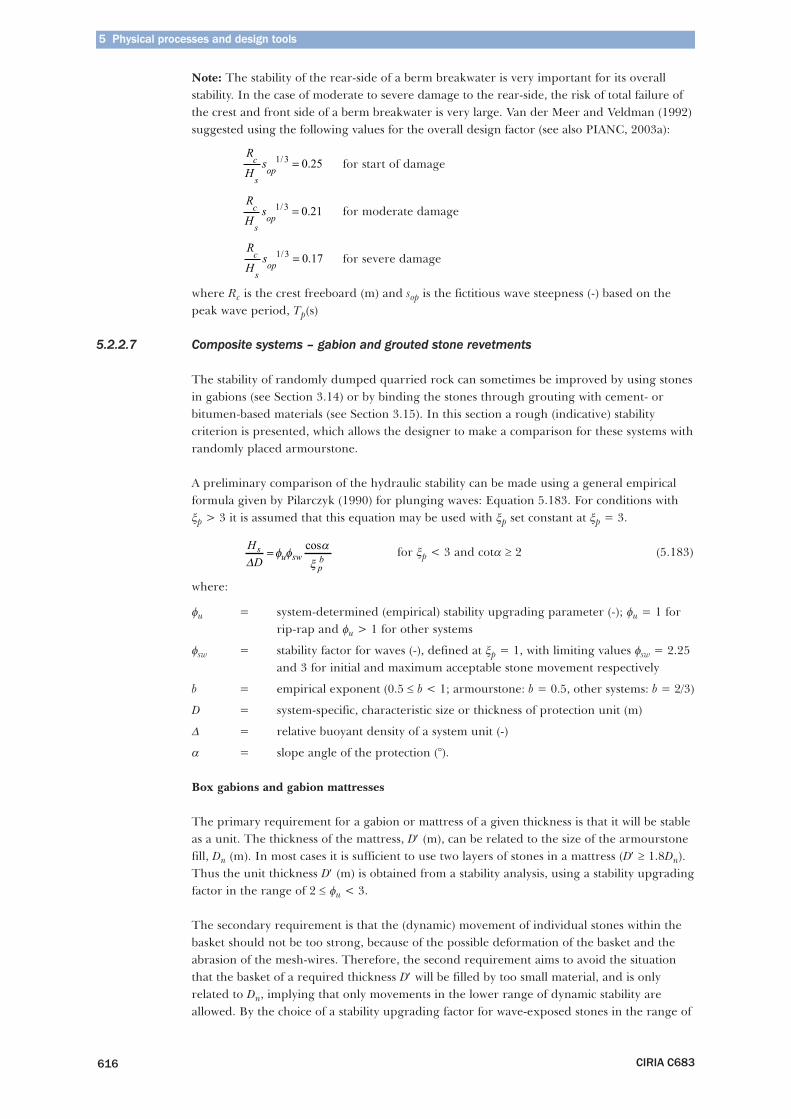
5 Physical processes and design tools
CIRIA C683616
Note: The stability of the rear-side of a berm breakwater is very important for its overallstability. In the case of moderate to severe damage to the rear-side, the risk of total failure ofthe crest and front side of a berm breakwater is very large. Van der Meer and Veldman (1992)suggested using the following values for the overall design factor (see also PIANC, 2003a):
for start of damage
for moderate damage
for severe damage
where Rc is the crest freeboard (m) and sop is the fictitious wave steepness (-) based on thepeak wave period, Tp(s)
5.2.2.7 Composite systems – gabion and grouted stone revetments
The stability of randomly dumped quarried rock can sometimes be improved by using stonesin gabions (see Section 3.14) or by binding the stones through grouting with cement- orbitumen-based materials (see Section 3.15). In this section a rough (indicative) stabilitycriterion is presented, which allows the designer to make a comparison for these systems withrandomly placed armourstone.
A preliminary comparison of the hydraulic stability can be made using a general empiricalformula given by Pilarczyk (1990) for plunging waves: Equation 5.183. For conditions withξp > 3 it is assumed that this equation may be used with ξp set constant at ξp = 3.
for ξp < 3 and cotα ≥ 2 (5.183)
where:
φu = system-determined (empirical) stability upgrading parameter (-); φu = 1 forrip-rap and φu > 1 for other systems
φsw = stability factor for waves (-), defined at ξp = 1, with limiting values φsw = 2.25and 3 for initial and maximum acceptable stone movement respectively
b = empirical exponent (0.5 ≤ b < 1; armourstone: b = 0.5, other systems: b = 2/3)
D = system-specific, characteristic size or thickness of protection unit (m)
Δ = relative buoyant density of a system unit (-)
α = slope angle of the protection (°).
Box gabions and gabion mattresses
The primary requirement for a gabion or mattress of a given thickness is that it will be stableas a unit. The thickness of the mattress, D′ (m), can be related to the size of the armourstonefill, Dn (m). In most cases it is sufficient to use two layers of stones in a mattress (D′ ≥ 1.8Dn).Thus the unit thickness D′ (m) is obtained from a stability analysis, using a stability upgradingfactor in the range of 2 ≤ φu < 3.
The secondary requirement is that the (dynamic) movement of individual stones within thebasket should not be too strong, because of the possible deformation of the basket and theabrasion of the mesh-wires. Therefore, the second requirement aims to avoid the situationthat the basket of a required thickness D′ will be filled by too small material, and is onlyrelated to Dn, implying that only movements in the lower range of dynamic stability areallowed. By the choice of a stability upgrading factor for wave-exposed stones in the range of
HDs
u swpbΔ
= φ φα
ξcos
R
Hsc
sop
1 3 0 25/ .=
R
Hsc
sop
1 3 0 21/ .=
R
Hsc
sop
1 3 0 17/ .=
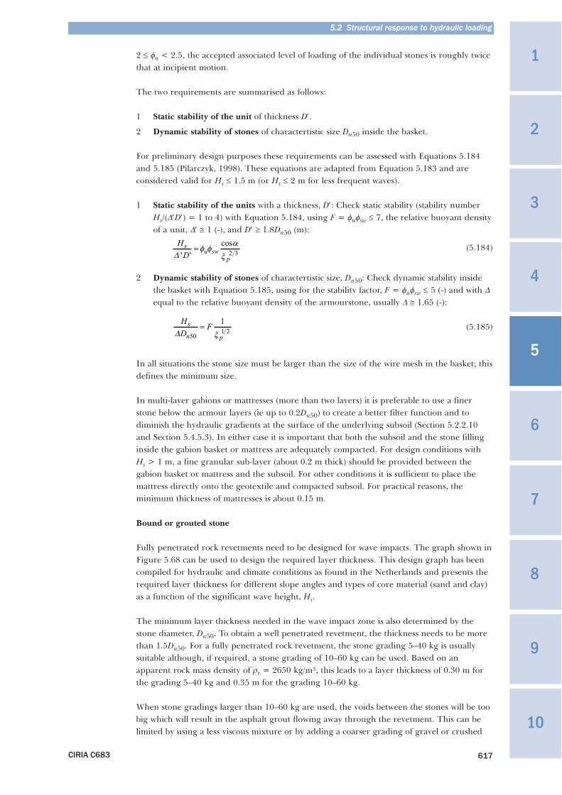
5.2 Structural response to hydraulic loading
CIRIA C683 617
1
3
4
10
9
8
7
6
5
2
2 ≤ φu < 2.5, the accepted associated level of loading of the individual stones is roughly twicethat at incipient motion.
The two requirements are summarised as follows:
1 Static stability of the unit of thickness D′.
2 Dynamic stability of stones of charactertistic size Dn50 inside the basket.
For preliminary design purposes these requirements can be assessed with Equations 5.184and 5.185 (Pilarczyk, 1998). These equations are adapted from Equation 5.183 and areconsidered valid for Hs ≤ 1.5 m (or Hs ≤ 2 m for less frequent waves).
1 Static stability of the units with a thickness, D′: Check static stability (stability numberHs/(Δ′D′) = 1 to 4) with Equation 5.184, using F = φuφsw ≤ 7, the relative buoyant densityof a unit, Δ′ ≅ 1 (-), and D′ ≥ 1.8Dn50 (m):
(5.184)
2 Dynamic stability of stones of charactertistic size, Dn50: Check dynamic stability insidethe basket with Equation 5.185, using for the stability factor, F = φuφsw ≤ 5 (-) and with Δequal to the relative buoyant density of the armourstone, usually Δ ≅ 1.65 (-):
(5.185)
In all situations the stone size must be larger than the size of the wire mesh in the basket; thisdefines the minimum size.
In multi-layer gabions or mattresses (more than two layers) it is preferable to use a finerstone below the armour layers (ie up to 0.2Dn50) to create a better filter function and todiminish the hydraulic gradients at the surface of the underlying subsoil (Section 5.2.2.10and Section 5.4.5.3). In either case it is important that both the subsoil and the stone fillinginside the gabion basket or mattress are adequately compacted. For design conditions withHs > 1 m, a fine granular sub-layer (about 0.2 m thick) should be provided between thegabion basket or mattress and the subsoil. For other conditions it is sufficient to place themattress directly onto the geotextile and compacted subsoil. For practical reasons, theminimum thickness of mattresses is about 0.15 m.
Bound or grouted stone
Fully penetrated rock revetments need to be designed for wave impacts. The graph shown inFigure 5.68 can be used to design the required layer thickness. This design graph has beencompiled for hydraulic and climate conditions as found in the Netherlands and presents therequired layer thickness for different slope angles and types of core material (sand and clay)as a function of the significant wave height, Hs.
The minimum layer thickness needed in the wave impact zone is also determined by thestone diameter, Dn50. To obtain a well penetrated revetment, the thickness needs to be morethan 1.5Dn50. For a fully penetrated rock revetment, the stone grading 5–40 kg is usuallysuitable although, if required, a stone grading of 10–60 kg can be used. Based on anapparent rock mass density of ρr = 2650 kg/m³, this leads to a layer thickness of 0.30 m forthe grading 5–40 kg and 0.35 m for the grading 10–60 kg.
When stone gradings larger than 10–60 kg are used, the voids between the stones will be toobig which will result in the asphalt grout flowing away through the revetment. This can belimited by using a less viscous mixture or by adding a coarser grading of gravel or crushed
HDs
u swpΔ ' '
cos= φ φα
ξ 2 3
HD
Fs
n pΔ 501 2
1=ξ
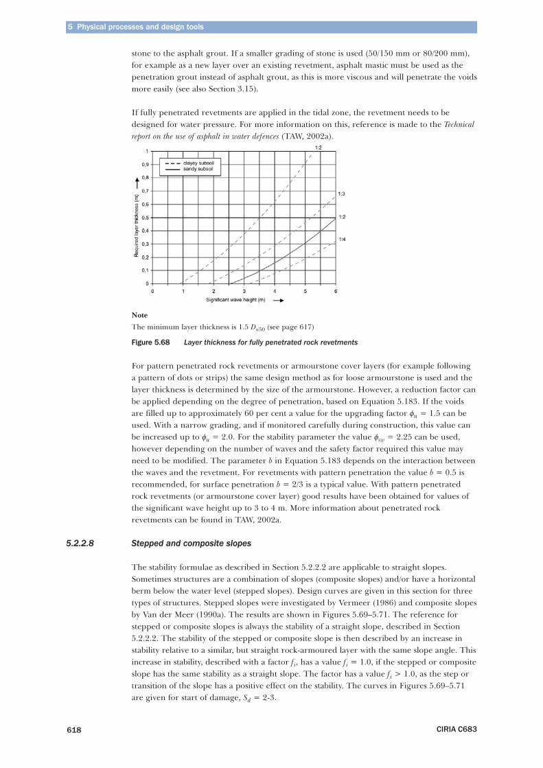
5 Physical processes and design tools
CIRIA C683618
stone to the asphalt grout. If a smaller grading of stone is used (50/150 mm or 80/200 mm),for example as a new layer over an existing revetment, asphalt mastic must be used as thepenetration grout instead of asphalt grout, as this is more viscous and will penetrate the voidsmore easily (see also Section 3.15).
If fully penetrated revetments are applied in the tidal zone, the revetment needs to bedesigned for water pressure. For more information on this, reference is made to the Technicalreport on the use of asphalt in water defences (TAW, 2002a).
Note
The minimum layer thickness is 1.5 Dn50 (see page 617)
Figure 5.68 Layer thickness for fully penetrated rock revetments
For pattern penetrated rock revetments or armourstone cover layers (for example followinga pattern of dots or strips) the same design method as for loose armourstone is used and thelayer thickness is determined by the size of the armourstone. However, a reduction factor canbe applied depending on the degree of penetration, based on Equation 5.183. If the voidsare filled up to approximately 60 per cent a value for the upgrading factor φu = 1.5 can beused. With a narrow grading, and if monitored carefully during construction, this value canbe increased up to φu = 2.0. For the stability parameter the value φsw = 2.25 can be used,however depending on the number of waves and the safety factor required this value mayneed to be modified. The parameter b in Equation 5.183 depends on the interaction betweenthe waves and the revetment. For revetments with pattern penetration the value b = 0.5 isrecommended, for surface penetration b = 2/3 is a typical value. With pattern penetratedrock revetments (or armourstone cover layer) good results have been obtained for values ofthe significant wave height up to 3 to 4 m. More information about penetrated rockrevetments can be found in TAW, 2002a.
5.2.2.8 Stepped and composite slopes
The stability formulae as described in Section 5.2.2.2 are applicable to straight slopes.Sometimes structures are a combination of slopes (composite slopes) and/or have a horizontalberm below the water level (stepped slopes). Design curves are given in this section for threetypes of structures. Stepped slopes were investigated by Vermeer (1986) and composite slopesby Van der Meer (1990a). The results are shown in Figures 5.69–5.71. The reference forstepped or composite slopes is always the stability of a straight slope, described in Section5.2.2.2. The stability of the stepped or composite slope is then described by an increase instability relative to a similar, but straight rock-armoured layer with the same slope angle. Thisincrease in stability, described with a factor fi, has a value fi = 1.0, if the stepped or compositeslope has the same stability as a straight slope. The factor has a value fi > 1.0, as the step ortransition of the slope has a positive effect on the stability. The curves in Figures 5.69–5.71are given for start of damage, Sd = 2-3.
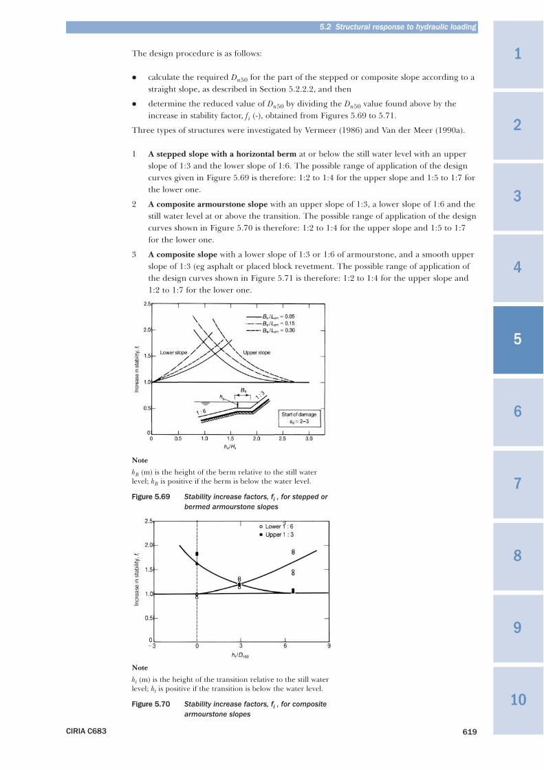
5.2 Structural response to hydraulic loading
CIRIA C683 619
1
3
4
10
9
8
7
6
5
2
The design procedure is as follows:
� calculate the required Dn50 for the part of the stepped or composite slope according to astraight slope, as described in Section 5.2.2.2, and then
� determine the reduced value of Dn50 by dividing the Dn50 value found above by theincrease in stability factor, fi (-), obtained from Figures 5.69 to 5.71.
Three types of structures were investigated by Vermeer (1986) and Van der Meer (1990a).
1 A stepped slope with a horizontal berm at or below the still water level with an upperslope of 1:3 and the lower slope of 1:6. The possible range of application of the designcurves given in Figure 5.69 is therefore: 1:2 to 1:4 for the upper slope and 1:5 to 1:7 forthe lower one.
2 A composite armourstone slope with an upper slope of 1:3, a lower slope of 1:6 and thestill water level at or above the transition. The possible range of application of the designcurves shown in Figure 5.70 is therefore: 1:2 to 1:4 for the upper slope and 1:5 to 1:7for the lower one.
3 A composite slope with a lower slope of 1:3 or 1:6 of armourstone, and a smooth upperslope of 1:3 (eg asphalt or placed block revetment. The possible range of application ofthe design curves shown in Figure 5.71 is therefore: 1:2 to 1:4 for the upper slope and1:2 to 1:7 for the lower one.
Note
hB (m) is the height of the berm relative to the still waterlevel; hB is positive if the berm is below the water level.
Figure 5.69 Stability increase factors, fi , for stepped orbermed armourstone slopes
Note
ht (m) is the height of the transition relative to the still waterlevel; ht is positive if the transition is below the water level.
Figure 5.70 Stability increase factors, fi , for compositearmourstone slopes
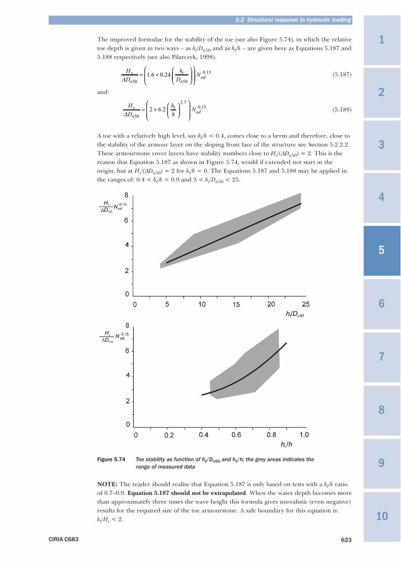
5.2 Structural response to hydraulic loading
CIRIA C683 623
1
3
4
10
9
8
7
6
5
2
The improved formulae for the stability of the toe (see also Figure 5.74), in which the relativetoe depth is given in two ways – as ht/Dn50 and as ht/h – are given here as Equations 5.187 and5.188 respectively (see also Pilarczyk, 1998).
(5.187)
and:
(5.188)
A toe with a relatively high level, say ht/h < 0.4, comes close to a berm and therefore, close tothe stability of the armour layer on the sloping front face of the structure see Section 5.2.2.2.These armourstone cover layers have stability numbers close to Hs/(ΔDn50) = 2. This is thereason that Equation 5.187 as shown in Figure 5.74, would if extended not start in theorigin, but at Hs/(ΔDn50) = 2 for ht/h = 0. The Equations 5.187 and 5.188 may be applied inthe ranges of: 0.4 < ht/h < 0.9 and 3 < ht/Dn50 < 25.
Figure 5.74 Toe stability as function of ht/Dn50 and ht/h; the grey areas indicates the range of measured data
NOTE: The reader should realise that Equation 5.187 is only based on tests with a ht/h ratioof 0.7–0.9. Equation 5.187 should not be extrapolated. When the water depth becomes morethan approximately three times the wave height this formula gives unrealistic (even negative)results for the required size of the toe armourstone. A safe boundary for this equation is:ht/Hs < 2.
HD
hD
Ns
n
t
nodΔ 50 50
0 151 6 0 24= +
⎛
⎝⎜⎜
⎞
⎠⎟⎟
⎛
⎝⎜⎜
⎞
⎠⎟⎟. .
.
HD
hh
Ns
n
todΔ 50
2 70 15
2 6 2= + ⎛⎝⎜
⎞⎠⎟
⎛
⎝⎜⎜
⎞
⎠⎟⎟
.
..
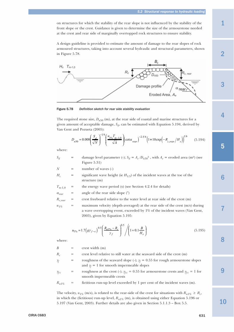
5.2 Structural response to hydraulic loading
CIRIA C683 631
1
3
4
10
9
8
7
6
5
2
on structures for which the stability of the rear slope is not influenced by the stability of thefront slope or the crest. Guidance is given to determine the size of the armourstone neededat the crest and rear side of marginally overtopped rock structures to ensure stability.
A design guideline is provided to estimate the amount of damage to the rear slopes of rockarmoured structures, taking into account several hydraulic and structural parameters, shownin Figure 5.78.
Figure 5.78 Definition sketch for rear side stability evaluation
The required stone size, Dn50 (m), at the rear side of coastal and marine structures for agiven amount of acceptable damage, Sd, can be estimated with Equation 5.194, derived byVan Gent and Pozueta (2005):
(5.194)
where:
Sd = damage level parameter (-); Sd = Ae /Dn50² , with Ae = eroded area (m²) (seeFigure 5.31)
N = number of waves (-)
Hs = significant wave height (ie H1/3) of the incident waves at the toe of thestructure (m)
Tm-1,0 = the energy wave period (s) (see Section 4.2.4 for details)
αrear = angle of the rear side slope (°)
Rc,rear = crest freeboard relative to the water level at rear side of the crest (m)
u1% = maximum velocity (depth-averaged) at the rear side of the crest (m/s) duringa wave overtopping event, exceeded by 1% of the incident waves (Van Gent,2003), given by Equation 5.195:
(5.195)
where:
B = crest width (m)
Rc = crest level relative to still water at the seaward side of the crest (m)
γf = roughness of the seaward slope (-); γf = 0.55 for rough armourstone slopesand γf = 1 for smooth impermeable slopes
γf-c = roughness at the crest (-); γf-c = 0.55 for armourstone crests and γf-c = 1 forsmooth impermeable crests
Ru1% = fictitious run-up level exceeded by 1 per cent of the incident waves (m).
The velocity, u1% (m/s), is related to the rear-side of the crest for situations with Ru1% ≥ Rc,in which the (fictitious) run-up level, Ru1% (m), is obtained using either Equation 5.196 or5.197 (Van Gent, 2003). Further details are also given in Section 5.1.1.3 – Box 5.5.
DS
N
u Tn
d mrear50
1 6
1 1 0 2 5 60 008 1=
⎛
⎝⎜⎜
⎞
⎠⎟⎟
⎛
⎝⎜⎜
⎞
⎠⎟⎟( )
−− −
. cot% , .
Δα ++ −( )( )10
1 6
exp,
R Hc rear s
u g R R BHf c
u c
f s1
0 51
0 5
1 7 1 0 1%
.%
.
. .= ( ) −⎛
⎝⎜⎜
⎞
⎠⎟⎟ +
⎛
⎝⎜
⎞
⎠⎟−γ
γ
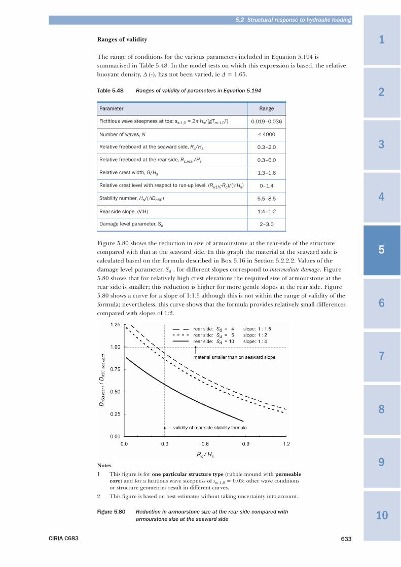
5.2 Structural response to hydraulic loading
CIRIA C683 633
1
3
4
10
9
8
7
6
5
2
Ranges of validity
The range of conditions for the various parameters included in Equation 5.194 issummarised in Table 5.48. In the model tests on which this expression is based, the relativebuoyant density, Δ (-), has not been varied, ie Δ = 1.65.
Table 5.48 Ranges of validity of parameters in Equation 5.194
Figure 5.80 shows the reduction in size of armourstone at the rear-side of the structurecompared with that at the seaward side. In this graph the material at the seaward side iscalculated based on the formula described in Box 5.16 in Section 5.2.2.2. Values of thedamage level parameter, Sd , for different slopes correspond to intermediate damage. Figure5.80 shows that for relatively high crest elevations the required size of armourstone at therear side is smaller; this reduction is higher for more gentle slopes at the rear side. Figure5.80 shows a curve for a slope of 1:1.5 although this is not within the range of validity of theformula; nevertheless, this curve shows that the formula provides relatively small differencescompared with slopes of 1:2.
Notes
1 This figure is for one particular structure type (rubble mound with permeablecore) and for a fictitious wave steepness of sm-1,0 = 0.03; other wave conditionsor structure geometries result in different curves.
2 This figure is based on best estimates without taking uncertainty into account.
Figure 5.80 Reduction in armourstone size at the rear side compared with armourstone size at the seaward side
Parameter Range
Fictitious wave steepness at toe: ss-1,0 = 2π Hs/(gTm-1,0²) 0.019–0.036
Number of waves, N < 4000
Relative freeboard at the seaward side, Rc/Hs 0.3–2.0
Relative freeboard at the rear side, Rc,rear/Hs 0.3–6.0
Relative crest width, B/Hs 1.3–1.6
Relative crest level with respect to run-up level, (Ru1%-Rc)/(γ Hs) 0–1.4
Stability number, Hs/(ΔDn50) 5.5–8.5
Rear-side slope, (V:H) 1:4–1:2
Damage level parameter, Sd 2–3.0
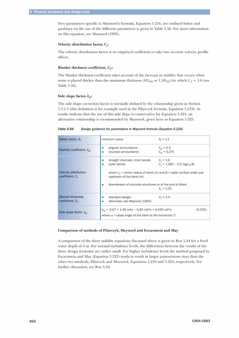
New parameters specific to Maynord’s formula, Equation 5.224, are outlined below andguidance on the use of the different parameters is given in Table 5.56. For more informationon this equation, see Maynord (1993).
Velocity distribution factor, Cv:
The velocity distribution factor is an empirical coefficient to take into account velocity profileeffects.
Blanket thickness coefficient, CT:
The blanket thickness coefficient takes account of the increase in stability that occurs whenstone is placed thicker than the minimum thickness (1D100 or 1.5D50) for which CT = 1.0 (seeTable 5.56).
Side slope factor, ksl:
The side slope correction factor is normally defined by the relationship given in Section5.2.1.3 (this definition is for example used in the Pilarczyk formula, Equation 5.219). Asresults indicate that the use of this side slope is conservative for Equation 5.224, analternative relationship is recommended by Maynord, given here as Equation 5.225.
Table 5.56 Design guidance for parameters in Maynord formula (Equation 5.224)
Comparison of methods of Pilarczyk, Maynord and Escarameia and May
A comparison of the three stability equations discussed above is given in Box 5.24 for a fixedwater depth of 4 m. For normal turbulence levels, the differences between the results of thethree design formulae are rather small. For higher turbulence levels the method proposed byEscarameia and May (Equation 5.223) tends to result in larger armourstone sizes than theother two methods, Pilarczyk and Maynord, Equations 5.219 and 5.224, respectively. Forfurther discussion, see Box 5.24.
5 Physical processes and design tools
CIRIA C683652
Safety factor, Sf minimum value: Sf = 1.1
Stability coefficient, Cst� angular armourstone: Cst = 0.3� rounded armourstone: Cst = 0.375
Velocity distributioncoefficient, Cv
� straight channels, inner bends: Cv = 1.0� outer bends: Cv = 1.283 – 0.2 log(rb/B)
where rb = centre radius of bend (m) and B = water surface width justupstream of the bend (m)
� downstream of concrete structures or at the end of dikes:Cv = 1.25
Blanket thicknesscoefficient, CT
� standard design: CT = 1.0� otherwise: see Maynord (1993)
Side slope factor, kslksl = -0.67 + 1.49 cotα – 0.45 cot²α + 0.045 cot³α (5.225)
where α = slope angle of the bank to the horizontal (º)
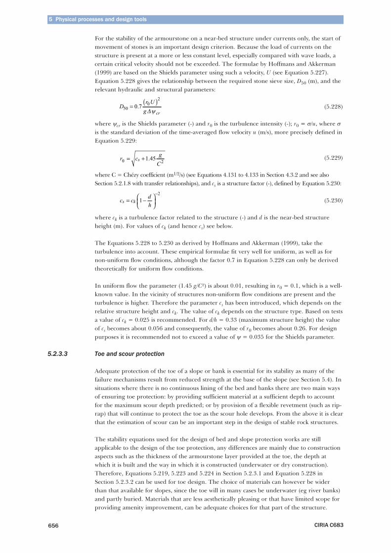
5 Physical processes and design tools
CIRIA C683656
For the stability of the armourstone on a near-bed structure under currents only, the start ofmovement of stones is an important design criterion. Because the load of currents on thestructure is present at a more or less constant level, especially compared with wave loads, acertain critical velocity should not be exceeded. The formulae by Hoffmans and Akkerman(1999) are based on the Shields parameter using such a velocity, U (see Equation 5.227).Equation 5.228 gives the relationship between the required stone sieve size, D50 (m), and therelevant hydraulic and structural parameters:
(5.228)
where ψcr is the Shields parameter (-) and r0 is the turbulence intensity (-); r0 = σ/u, where σis the standard deviation of the time-averaged flow velocity u (m/s), more precisely defined inEquation 5.229:
(5.229)
where C = Chézy coefficient (m1/2/s) (see Equations 4.131 to 4.133 in Section 4.3.2 and see alsoSection 5.2.1.8 with transfer relationships), and cs is a structure factor (-), defined by Equation 5.230:
(5.230)
where ck is a turbulence factor related to the structure (-) and d is the near-bed structureheight (m). For values of ck (and hence cs) see below.
The Equations 5.228 to 5.230 as derived by Hoffmans and Akkerman (1999), take theturbulence into account. These empirical formulae fit very well for uniform, as well as fornon-uniform flow conditions, although the factor 0.7 in Equation 5.228 can only be derivedtheoretically for uniform flow conditions.
In uniform flow the parameter (1.45 g/C²) is about 0.01, resulting in r0 = 0.1, which is a well-known value. In the vicinity of structures non-uniform flow conditions are present and theturbulence is higher. Therefore the parameter cs has been introduced, which depends on therelative structure height and ck. The value of ck depends on the structure type. Based on testsa value of ck = 0.025 is recommended. For d/h = 0.33 (maximum structure height) the valueof cs becomes about 0.056 and consequently, the value of r0 becomes about 0.26. For designpurposes it is recommended not to exceed a value of ψ = 0.035 for the Shields parameter.
5.2.3.3 Toe and scour protection
Adequate protection of the toe of a slope or bank is essential for its stability as many of thefailure mechanisms result from reduced strength at the base of the slope (see Section 5.4). Insituations where there is no continuous lining of the bed and banks there are two main waysof ensuring toe protection: by providing sufficient material at a sufficient depth to accountfor the maximum scour depth predicted; or by provision of a flexible revetment (such as rip-rap) that will continue to protect the toe as the scour hole develops. From the above it is clearthat the estimation of scour can be an important step in the design of stable rock structures.
The stability equations used for the design of bed and slope protection works are stillapplicable to the design of the toe protection, any differences are mainly due to constructionaspects such as the thickness of the armourstone layer provided at the toe, the depth atwhich it is built and the way in which it is constructed (underwater or dry construction).Therefore, Equations 5.219, 5.223 and 5.224 in Section 5.2.3.1 and Equation 5.228 inSection 5.2.3.2 can be used for toe design. The choice of materials can however be widerthan that available for slopes, since the toe will in many cases be underwater (eg river banks)and partly buried. Materials that are less aesthetically pleasing or that have limited scope forproviding amenity improvement, can be adequate choices for that part of the structure.
Dr U
g cr50
02
0 7=( )
.Δψ
r0 = +c gC
s 1 452
.
c c dh
s k= −⎛⎝⎜
⎞⎠⎟
−1
2
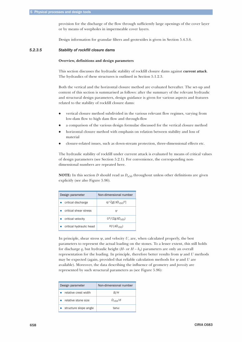
5 Physical processes and design tools
CIRIA C683658
provision for the discharge of the flow through sufficiently large openings of the cover layeror by means of weepholes in impermeable cover layers.
Design information for granular filters and geotextiles is given in Section 5.4.3.6.
5.2.3.5 Stability of rockfill closure dams
Overview, definitions and design parameters
This section discusses the hydraulic stability of rockfill closure dams against current attack.The hydraulics of these structures is outlined in Section 5.1.2.3.
Both the vertical and the horizontal closure method are evaluated hereafter. The set-up andcontent of this section is summarised as follows: after the summary of the relevant hydraulicand structural design parameters, design guidance is given for various aspects and featuresrelated to the stability of rockfill closure dams:
� vertical closure method subdivided in the various relevant flow regimes, varying fromlow-dam flow to high dam flow and through-flow
� a comparison of the various design formulae discussed for the vertical closure method
� horizontal closure method with emphasis on relation between stability and loss ofmaterial
� closure-related issues, such as down-stream protection, three-dimensional effects etc.
The hydraulic stability of rockfill under current attack is evaluated by means of critical valuesof design parameters (see Section 5.2.1). For convenience, the corresponding non-dimensional numbers are repeated here.
NOTE: In this section D should read as Dn50 throughout unless other definitions are givenexplicitly (see also Figure 5.96).
In principle, shear stress ψ, and velocity U, are, when calculated properly, the bestparameters to represent the actual loading on the stones. To a lesser extent, this still holdsfor discharge q, but hydraulic height (H- or H – hb) parameters are only an overallrepresentation for the loading. In principle, therefore better results from ψ and U methodsmay be expected (again, provided that reliable calculation methods for ψ and U areavailable). Moreover, the data describing the influence of geometry and porosity arerepresented by such structural parameters as (see Figure 5.96):
Design parameter Non-dimensional number
� relative crest width B/H
� relative stone size Dn50/d
� structure slope angle tanα
Design parameter Non-dimensional number
� critical discharge q/√[g(ΔDn50)³]
� critical shear stress ψ
� critical velocity U²/(2gΔDn50)
� critical hydraulic head H/(ΔDn50)
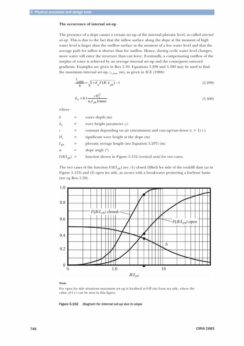
5 Physical processes and design tools
CIRIA C683746
The occurrence of internal set-up
The presence of a slope causes a certain set-up of the internal phreatic level, so called internalset-up. This is due to the fact that the inflow surface along the slope at the moment of highwater level is larger than the outflow surface at the moment of a low water level and that theaverage path for inflow is shorter than for outflow. Hence, during cyclic water level changes,more water will enter the structure than can leave. Eventually, a compensating outflow of thesurplus of water is achieved by an average internal set-up and the consequent outwardgradients. Examples are given in Box 5.39. Equations 5.299 and 5.300 may be used to findthe maximum internal set-up, zs,max (m), as given in ICE (1988):
(5.299)
(5.300)
where:
h = water depth (m)
δw = wave height parameter (-)
c = constant depending on air entrainment and run-up/run-down (c > 1) (-)
Hs = significant wave height at the slope (m)
Lph = phreatic storage length (see Equation 5.297) (m)
α = slope angle (°)
F(B/Lph) = function shown in Figure 5.152 (vertical axis) for two cases.
The two cases of the function F(B/Lph) are: (1) closed (filled) lee side of the rockfill dam (as inFigure 5.153) and (2) open lee side, as occurs with a breakwater protecting a harbour basin(see eg Box 5.39).
Note
For open lee side situations maximum set-up is localised at b⋅B (m) from sea side, where the value of b (-) can be seen in this figure.
Figure 5.152 Diagram for internal set-up due to slope
z
hF B Ls,max
w ph= + −1 1δ ( / )
δαw
s
v ph
cHn L h
= 0 12
.tan
The set-up is particularly high (up to 0.5 times the wave height), if only reverse drainage(outflow) is possible, back towards the sea. This may be because Lph << B or because the leeside of the rockfill structure is hydraulically closed, eg when a sand backfill behind abreakwater or seawall (see Figure 5.153).
Figure 5.153 Internal phreatic set-up due to backfill
Box 5.39 Typical examples of internal phreatic set-up
Pore pressures dominated by elastic storage
In this section, attention is given to the effects of the elastic compressibility of both the porefluid and the skeleton. Varying pore pressures cause some variations of the volume of thepore fluid. This variation is very small if the pore fluid is pure water without any air in it,because water is practically incompressible. However, in the region of varying water level, thepore water does contain air and the resulting compressibility may be large enough tocontribute to a sequential flow of water in and out the soil mass, according to the followingmechanism:
� varying effective stresses, σ′ , result in variation of the pore volume caused bycompression of the skeleton, which in turn forces pore water to flow in and out of thesoil (or rockfill) mass. This flow in and out because of compression of air-containing porewater and/or grain skeleton is called consolidation.
When the rate of pressure changes along the external boundary becomes so quick thatconsolidation in the soil cannot take place completely, then elastic storage plays a role. Itmeans that the change of pore pressure and/or effective stress is retarded by the fact that therequired outflow of pore water is not possible. The soil (water/air) system has too long apermeability (low k-value of soil) and/or possesses too low a stiffness; the modulus ofcompression of the water/air, Kwa (= Δp/(ΔV/V) and the mve-value of the soil, being the elasticcoefficient of volume change) in relation to the rate of boundary pressure changes (fordefinitions and descriptions, see Section 5.4.4.4).
5.3 Modelling of hydraulic interactions and structural response
CIRIA C683
5.4 Geotechnical design
Two examples of internal set-up are given:
1. Rockfill dike (coarse armourstone) around a lake or harbour basin
Cross-sectional and structural data are: tanα = 1:3, B = 30 m, h = 10 m, nv = 0.4 and k = 0.1 m/s.The loading by (short) wind waves is characterised by Hs = 4 m and T = 4.5 s.
Using these data in the Equations 5.296 and 5.297 gives: Tph = 1100 s, Lph = 1.9 m and consequently,B/Lph = 16, F(B/Lph) = 0.75 and b = 0.19 (Figure 5.152). Further, substituting c = 1 in Equation 5.300gives: δw = 0.63, finally resulting in: zs,max = 2 m (by applying Equation 5.299), occurring at an approximatedistance of 6 m from the waterfront.
2. The same dike and loading as under 1 above, but with a backfill of sand
In this case: Tph = 1100 s, Lph = 1.9 m, F(B/Lph) = 1 (Figure 5.152) and δw = 0.63. Consequently, zs,max =2.7 m, occurring approximately at the boundary with the backfill.
747
1
3
4
10
9
8
7
6
5
2
5 Physical processes and design tools
CIRIA C683772
Yamamoto, T, Koning, H L, Sellmeijer, H and van Hijum, E (1978). “On the response of aporo-elastic bed to water waves”. J Fluid Mech, vol 87, Jul, pp 193–206
Youd, T L, Idriss, I M, Andrus, R D, Arango, I, Castro, G, Christian, J T, Dobry, R, LiamFinn, W D L, Harder, L F, Hynes, M E, Ishihara, K, Koester, J P, Liao, S S C, Marcuson III,W F, Martin, G R, Mitchell, J K, Moriwaki, Y, Power, M S, Robertson, P K, Seed, R B andStokoe II, K H (2001). “Liquefaction resistance of soils: summary report from the 1996NCEER and 1998 NCEER/NSF workshops on evaluation of liquefaction resistance of soils”. JGeotech and Geo-env Engg, vol 127, no 10, pp 817–833
5.5.1 Standards
British standards
British Standards Institution, London
BS 6349-7:1991. Maritime structures. Guide to the design and construction of breakwaters
Canadian standards
Canadian Standards Association, Rexdale, Ont
CSA-S471-04 (2004). Design, construction and installation of fixed offshore structures. Part I: generalrequirements, design criteria, the environment, and loads
European standards
Eurocode 7 – see EN 1997-1:2004 and EN 1997-2
Eurocode 8 – see EN 1998-1:2004 and EN 1998-5:2004
EN 1997-1:2004. Eurocode 7. Geotechnical design. General rules
EN 1997-2 Geotechnical design. Ground investigations. Lab testing
EN 1197-2 Geotechnical design. Ground investigation and testing
EN ISO 11058:1999. Geotextiles and geotextile-related products. Determination of water permeabilitycharacteristics normal to the plane, without load
EN ISO 12956:1999. Geotextiles and geotextile-related products. Determination of the characteristicopening size
EN 1998-1:2004 Eurocode 8. Design of structures for earthquake resistance. General rules, seismicactions and rules for building
EN 1998-5:2004 Eurocode 8. Design of structures for earthquake resistance. Foundations, retainingstructures and geotechnical aspects
French standards
Association Française de Normalisation (AFNOR), La Plaine Saint-Denis
NF G38-061:1993. Recommendations for the use of geotextiles and geotextile-related products.Determination of the hydraulic properties and installation of geotextiles and geotextile-related products infiltration and drainage systems
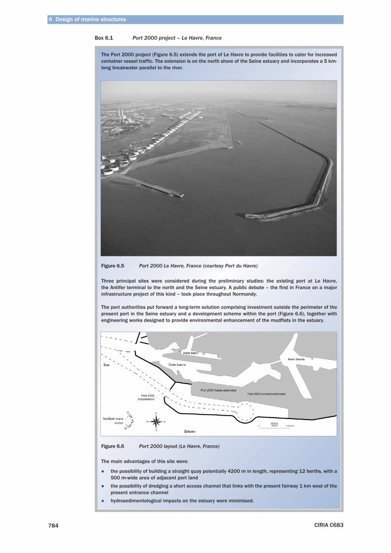
6 Design of marine structures
CIRIA C683784
Box 6.1 Port 2000 project – Le Havre, France
The Port 2000 project (Figure 6.5) extends the port of Le Havre to provide facilities to cater for increasedcontainer vessel traffic. The extension is on the north shore of the Seine estuary and incorporates a 5 km-long breakwater parallel to the river.
Figure 6.5 Port 2000 Le Havre, France (courtesy Port du Havre)
Three principal sites were considered during the preliminary studies: the existing port at Le Havre, the Antifer terminal to the north and the Seine estuary. A public debate – the first in France on a majorinfrastructure project of this kind – took place throughout Normandy.
The port authorities put forward a long-term solution comprising investment outside the perimeter of thepresent port in the Seine estuary and a development scheme within the port (Figure 6.6), together withengineering works designed to provide environmental enhancement of the mudflats in the estuary.
Figure 6.6 Port 2000 layout (Le Havre, France)
The main advantages of this site were:
� the possibility of building a straight quay potentially 4200 m in length, representing 12 berths, with a500 m-wide area of adjacent port land
� the possibility of dredging a short access channel that links with the present fairway 1 km west of thepresent entrance channel
� hydrosedimentological impacts on the estuary were minimised.
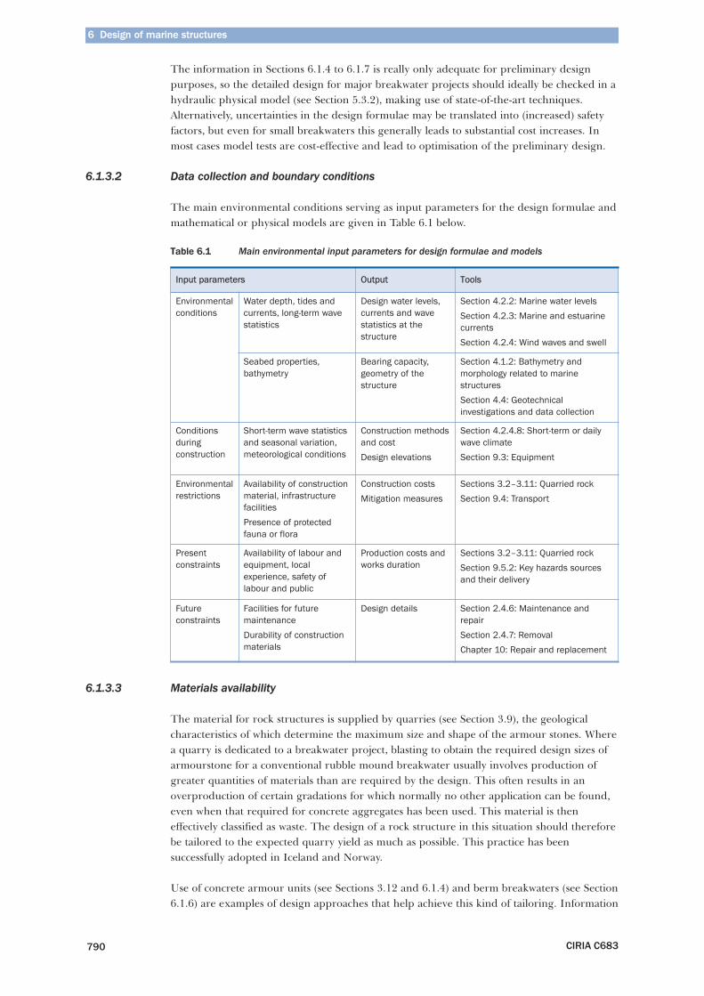
6 Design of marine structures
CIRIA C683790
The information in Sections 6.1.4 to 6.1.7 is really only adequate for preliminary designpurposes, so the detailed design for major breakwater projects should ideally be checked in ahydraulic physical model (see Section 5.3.2), making use of state-of-the-art techniques.Alternatively, uncertainties in the design formulae may be translated into (increased) safetyfactors, but even for small breakwaters this generally leads to substantial cost increases. Inmost cases model tests are cost-effective and lead to optimisation of the preliminary design.
6.1.3.2 Data collection and boundary conditions
The main environmental conditions serving as input parameters for the design formulae andmathematical or physical models are given in Table 6.1 below.
Table 6.1 Main environmental input parameters for design formulae and models
6.1.3.3 Materials availability
The material for rock structures is supplied by quarries (see Section 3.9), the geologicalcharacteristics of which determine the maximum size and shape of the armour stones. Wherea quarry is dedicated to a breakwater project, blasting to obtain the required design sizes ofarmourstone for a conventional rubble mound breakwater usually involves production ofgreater quantities of materials than are required by the design. This often results in anoverproduction of certain gradations for which normally no other application can be found,even when that required for concrete aggregates has been used. This material is theneffectively classified as waste. The design of a rock structure in this situation should thereforebe tailored to the expected quarry yield as much as possible. This practice has beensuccessfully adopted in Iceland and Norway.
Use of concrete armour units (see Sections 3.12 and 6.1.4) and berm breakwaters (see Section6.1.6) are examples of design approaches that help achieve this kind of tailoring. Information
Input parameters Output Tools
Environmentalconditions
Water depth, tides andcurrents, long-term wavestatistics
Design water levels,currents and wavestatistics at thestructure
Section 4.2.2: Marine water levels
Section 4.2.3: Marine and estuarinecurrents
Section 4.2.4: Wind waves and swell
Seabed properties,bathymetry
Bearing capacity,geometry of thestructure
Section 4.1.2: Bathymetry andmorphology related to marinestructures
Section 4.4: Geotechnicalinvestigations and data collection
Conditionsduringconstruction
Short-term wave statisticsand seasonal variation,meteorological conditions
Construction methodsand cost
Design elevations
Section 4.2.4.8: Short-term or dailywave climate
Section 9.3: Equipment
Environmentalrestrictions
Availability of constructionmaterial, infrastructurefacilities
Presence of protectedfauna or flora
Construction costs
Mitigation measures
Sections 3.2–3.11: Quarried rock
Section 9.4: Transport
Presentconstraints
Availability of labour andequipment, localexperience, safety oflabour and public
Production costs andworks duration
Sections 3.2–3.11: Quarried rock
Section 9.5.2: Key hazards sourcesand their delivery
Futureconstraints
Facilities for futuremaintenance
Durability of constructionmaterials
Design details Section 2.4.6: Maintenance andrepair
Section 2.4.7: Removal
Chapter 10: Repair and replacement
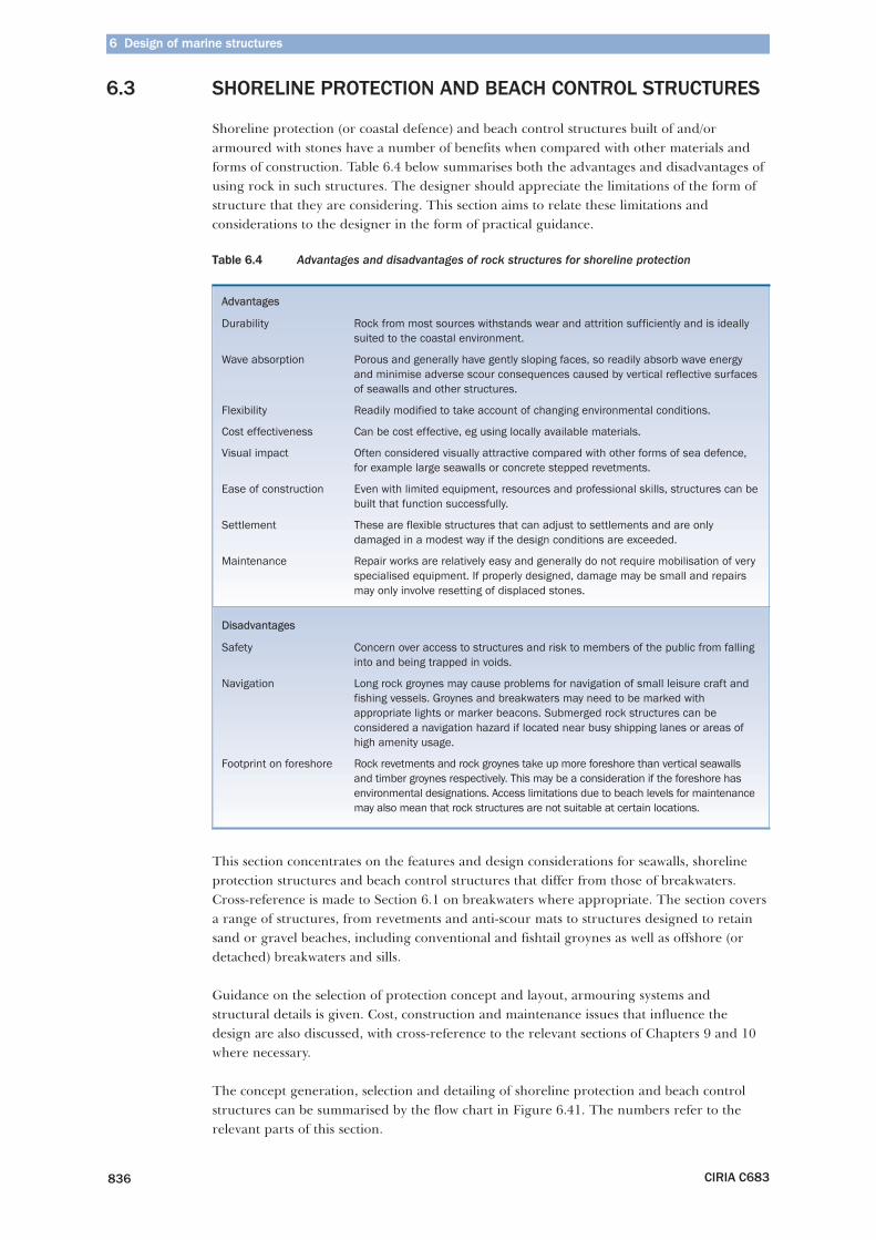
6 Design of marine structures
CIRIA C683836
6.3 SHORELINE PROTECTION AND BEACH CONTROL STRUCTURES
Shoreline protection (or coastal defence) and beach control structures built of and/orarmoured with stones have a number of benefits when compared with other materials andforms of construction. Table 6.4 below summarises both the advantages and disadvantages ofusing rock in such structures. The designer should appreciate the limitations of the form ofstructure that they are considering. This section aims to relate these limitations andconsiderations to the designer in the form of practical guidance.
Table 6.4 Advantages and disadvantages of rock structures for shoreline protection
This section concentrates on the features and design considerations for seawalls, shorelineprotection structures and beach control structures that differ from those of breakwaters.Cross-reference is made to Section 6.1 on breakwaters where appropriate. The section coversa range of structures, from revetments and anti-scour mats to structures designed to retainsand or gravel beaches, including conventional and fishtail groynes as well as offshore (ordetached) breakwaters and sills.
Guidance on the selection of protection concept and layout, armouring systems andstructural details is given. Cost, construction and maintenance issues that influence thedesign are also discussed, with cross-reference to the relevant sections of Chapters 9 and 10where necessary.
The concept generation, selection and detailing of shoreline protection and beach controlstructures can be summarised by the flow chart in Figure 6.41. The numbers refer to therelevant parts of this section.
Advantages
Durability Rock from most sources withstands wear and attrition sufficiently and is ideallysuited to the coastal environment.
Wave absorption Porous and generally have gently sloping faces, so readily absorb wave energyand minimise adverse scour consequences caused by vertical reflective surfacesof seawalls and other structures.
Flexibility Readily modified to take account of changing environmental conditions.
Cost effectiveness Can be cost effective, eg using locally available materials.
Visual impact Often considered visually attractive compared with other forms of sea defence,for example large seawalls or concrete stepped revetments.
Ease of construction Even with limited equipment, resources and professional skills, structures can bebuilt that function successfully.
Settlement These are flexible structures that can adjust to settlements and are onlydamaged in a modest way if the design conditions are exceeded.
Maintenance Repair works are relatively easy and generally do not require mobilisation of veryspecialised equipment. If properly designed, damage may be small and repairsmay only involve resetting of displaced stones.
Disadvantages
Safety Concern over access to structures and risk to members of the public from fallinginto and being trapped in voids.
Navigation Long rock groynes may cause problems for navigation of small leisure craft andfishing vessels. Groynes and breakwaters may need to be marked withappropriate lights or marker beacons. Submerged rock structures can beconsidered a navigation hazard if located near busy shipping lanes or areas ofhigh amenity usage.
Footprint on foreshore Rock revetments and rock groynes take up more foreshore than vertical seawallsand timber groynes respectively. This may be a consideration if the foreshore hasenvironmental designations. Access limitations due to beach levels for maintenancemay also mean that rock structures are not suitable at certain locations.
6 Design of marine structures
CIRIA C683860
combinations should be investigated to assess scour depth and toe stability – the worst caseconditions may occur at a low water level even though wave heights may be lower.Consideration should also be given to the full life of the structure, ie to take account ofnatural foreshore changes and potentially increased wave activity at the end of the serviceperiod. For most coastal structures, wave forces (downrush and breaking) present the criticalconditions when determining stability of the toe. However, currents can become important,particularly in deeper water or more sheltered sites where wave activity is restricted.
In summary the important considerations in establishing the nature of toe protectionrequired are:
� location of the structure (scour is most severe near the wave-break point)
� form of structure (wave forces produced as a result of reflectivity or downrush)
� nature of the bed (resistance to erosion and grain size)
� nature of structure, revetment, breakwater etc.
As a general rule, scour potential is greatest where the water depth at the toe is less thantwice the height of the maximum unbroken wave.
Special attention should also be given to areas where scour may be intensified, such aschanges in alignment, structure roundheads, channels and downdrift of groynes etc.
Design methods for scour and toe protection are presented in Section 5.2.2.9.
Depth and form of toe detail
The basic principle of flexible toe protection is to provide an extension of the armour facesuch that the foundation material is kept in place beneath the structure to the bottom of themaximum depth of scour. Caution should be exercised if a non-flexible toe protection is to beadopted as this will not accommodate any change in profile if scour is to occur, which maylead to brittle failure.
When placing stones in a situation where the toe is below low water the construction aspectscovered in Section 9.7.1.2 should be considered. The use of geotextiles should be carefullyconsidered prior to their inclusion in a design with respect to installation, also covered inSection 9.7.1.2. Consultation with experienced installers and manufacturers should helpassess the feasibility and cost benefits of using them. Consideration should be given towhether suitable granular underlayers and filters can be used instead.
A range of toe details are presented in Figures 6.57 to 6.64 for the following ground conditions.
1 Rock foreshore.
2 Impermeable layer near foreshore level.
3 Sand/gravel foreshore.
Different construction scenarios are discussed below. The list of examples is not exhaustiveand there may be situations where a combination of the examples shown may be applicable.
The toe details shown in Figures 6.59–6.64 indicate that a geotextile may be necessary whereconstruction is to take place on a granular material, to prevent loss of bed material throughthe structure. The designer should check whether a geotextile is required to ensure interfacestability criteria between adjacent granular layers are met (see Section 5.4.3.6). This appliesto the transition between the bed material and the placed layers (core or underlayer) andalso between adjacent layers within the structure, for example between the underlayer andthe core.
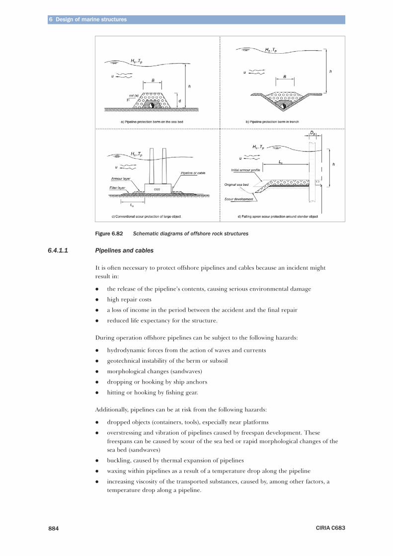
6 Design of marine structures
CIRIA C683884
Figure 6.82 Schematic diagrams of offshore rock structures
6.4.1.1 Pipelines and cables
It is often necessary to protect offshore pipelines and cables because an incident mightresult in:
� the release of the pipeline’s contents, causing serious environmental damage
� high repair costs
� a loss of income in the period between the accident and the final repair
� reduced life expectancy for the structure.
During operation offshore pipelines can be subject to the following hazards:
� hydrodynamic forces from the action of waves and currents
� geotechnical instability of the berm or subsoil
� morphological changes (sandwaves)
� dropping or hooking by ship anchors
� hitting or hooking by fishing gear.
Additionally, pipelines can be at risk from the following hazards:
� dropped objects (containers, tools), especially near platforms
� overstressing and vibration of pipelines caused by freespan development. Thesefreespans can be caused by scour of the sea bed or rapid morphological changes of thesea bed (sandwaves)
� buckling, caused by thermal expansion of pipelines
� waxing within pipelines as a result of a temperature drop along the pipeline
� increasing viscosity of the transported substances, caused by, among other factors, atemperature drop along a pipeline.
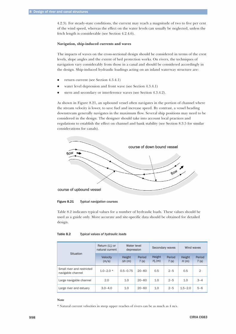
8 Design of river and canal structures
CIRIA C683998
4.2.3). For steady-state conditions, the current may reach a magnitude of two to five per centof the wind speed, whereas the effect on the water levels can usually be neglected, unless thefetch length is considerable (see Section 4.2.4.6).
Navigation, ship-induced currents and waves
The impacts of waves on the cross-sectional design should be considered in terms of the crestlevels, slope angles and the extent of bed protection works. On rivers, the techniques ofnavigation vary considerably from those in a canal and should be considered accordingly inthe design. Ship-induced hydraulic loadings acting on an inland waterway structure are:
� return current (see Section 4.3.4.1)
� water level depression and front wave (see Section 4.3.4.1)
� stern and secondary or interference waves (see Section 4.3.4.2).
As shown in Figure 8.21, an upbound vessel often navigates in the portion of channel wherethe stream velocity is lower, to save fuel and increase speed. By contrast, a vessel headingdownstream generally navigates in the maximum flow. Several ship positions may need to beconsidered in the design. The designer should take into account local practices andregulations to establish the effect on channel and bank stability (see Section 8.3.5 for similarconsiderations for canals).
Figure 8.21 Typical navigation courses
Table 8.2 indicates typical values for a number of hydraulic loads. These values should beused as a guide only. More accurate and site-specific data should be obtained for detaileddesign.
Table 8.2 Typical values of hydraulic loads
Note
* Natural current velocities in steep upper reaches of rivers can be as much as 4 m/s.
Situation
Return (Ur) ornatural current
Water leveldepression
Secondary waves Wind waves
Velocity(m/s)
HeightΔh (m)
PeriodT (s)
HeightHi (m)
PeriodT (s)
HeightH (m)
PeriodT (s)
Small river and restrictednavigable channel
1.0–2.0 * 0.5–0.75 20–60 0.5 2–5 0.5 2
Large navigable channel 2.0 1.0 20–60 1.0 2–5 1.0 3–4
Large river and estuary 3.0–4.0 1.0 20–60 1.0 2–5 1.5–2.0 5–6
8.2 River training works
CIRIA C683 999
Ice loads
The resistance of river training works against the forces exerted by ice is of particularimportance, eg along the shores of lakes and large rivers in arctic areas. The specificproblems that have to be solved in such conditions are highlighted here. Ice riding up theembankment slope may damage the armour layer and in some instances the horizontal forcesmay become so large that the top part of a guide bund or dike is pushed backwards –inducing decapitation.
NOTE: Considerations for design with ice loads
In fact, ice has both beneficial and detrimental effects. On one hand the presence of ice limitsthe wave climate and erosion. On the other hand, ice can damage slope protection, and canride up and damage surface facilities. Breakwaters designed to withstand wave attack areoften able to withstand ice forces. However, there is a delicate balance between thesmoothness required to encourage ice bending (to minimise the ice load and movement ofindividual stones) and the roughness required to dissipate wave energy.
Armourstone can be subject to normal and shear stresses along the surface. These stresseswill introduce a rotation, dislodging the individual stones. It is therefore desirable that thesurface of the armourstone is relatively smooth and the stone layer is well keyed. Angularstones tend to nest together and interlock. The friction coefficient of ice on rock slopes variesbetween 0.1 and 0.5. It is obvious that smoother stone surfaces reduce the shear stress. Anotherdisadvantage of a rough slope with relatively large surfaces of individual stones is the possibilityof rigidly frozen ice that can remove the armourstone and float it away from the site.
From experience with ice and armourstone in bank protection works several rules of thumbcan be defined:
� widely graded armourstone (or rip-rap) should be avoided; standard heavy gradings arepreferred (see Section 3.4.3)
� for about 0.7 m thick ice, a standard heavy grading of 300–1000 kg or greater should be used
� generally, when there are significant water level changes and concerns over plucking outof individual stones, the median nominal stone size, Dn50 (m), should exceed themaximum ice thickness, tice;max (m)
� the slope of the armour layer should be less than 30° to minimise the shear stress
� slopes below the waterline should be less steep than slopes above the waterline toencourage rubbling and prevent ice ride-up.
Further reference is made to Section 5.2.4 and McDonald (1988), and Wuebben (1995).
Designing with the above rules of thumb in mind often implies that conflicts (of interest)arise: stability requirements lead to angular, relatively heavy stone as armouring of therevetment, whereas coping with the ice loading effects leads to a smooth surface. In that casealternative materials may be attractive, such as some types of concrete armour units (seeSections 3.12 and 5.2.2.3), concrete block or gabion mattresses, and grouted stone (seeSection 3.15, 5.2.2.7 and 8.6.2).
1
3
4
10
9
8
7
6
5
2
8.2 River training works
CIRIA C683 1003
� where the water level has the potential to fall rapidly after being high for some time.This can destabilise the bank because the ground mass is saturated
� where the risk of slip failure is important, eg where the foundation soils are looselydeposited or where mica is present.
When a gentle slope cannot be achieved, alternatives should be considered and use ofgabions to form a retaining wall may be considered.
Where a revetment is constructed in two or more levels, usually separated by a berm (seeFigure 8.10), different slopes and types of armouring can be adopted for each of the levels.For instance, in a river environment, the upper layers of the protected soil mass may beloosely packed and more vulnerable to liquefaction in the case of earthquakes than otherlower layers. The situation can be remedied by introducing a gentler slope in the upper partof the revetment. Conversely, in situations where the riverbank comprises loose sandymaterial overlain by layers of clay, it may be necessary to have a less steep slope on the lowerpart of the revetment.
Crest level
The crest level of a revetment is normally set above the design flood level with freeboard inthe order of 0.3 to 0.5 m. Larger values can be adopted in very large rivers or where waverun-up is expected. In summary, the crest level of revetments and river dikes is determined by:
� design water (= flood) level, which should be based on the probabilistic approach ofboth the river run-off discharge, the highest tidal level (HWS) in estuaries, and the windset-up in estuaries and lakes (see Sections 4.2 and 4.3)
� wave run-up for which the two per cent exceedance level is often applied; this leveldepends on slope angle, slope roughness,existence of a berm, permeability of thestructure, wave height and – period, and the angle of wave attack (see Section 5.1.1.3)
� a margin to take into account the effects of seiches (see Section 4.2) and gust bumps(single waves) resulting from a sudden violent wind rush), which may vary from a fewtens of centimetres to a few metres (for seiches)
� a rise of the mean sea level due to climate changes (see Section 4.2), which applies toestuaries and locations along rivers close to the sea
� settlement of the subsoil adn the structure itself during its lifetime (see Section 5.4)
The combination of the above factors in a probabilistic approach defines the crest level; thefreeboard, Rc (m), relative to the design water level depends on the last four of the five listedfactors above.
There are circumstances where the crest level of the revetment does not need to be as high asthe flood level, notably for some spur-dikes that are overtopped in floods (see Section 8.2.7.1).It is also possible for a revetment to have the critical hydraulic loading occurring at standardwater levels due to currents or waves, whereas loading in flood conditions is less severe.
Berm
A berm may be designed on the slope between the lower part and the upper part of therevetment (see Figure 8.10). A berm may be required to improve the overall stability of theworks and as an alternative to flattening the face slope of the whole revetment. It may alsoform a transition between parts of the revetment using different types of materials or placingtechniques. It may also be a means to reduce run-up when this is critical.
1
3
4
10
9
8
7
6
5
2
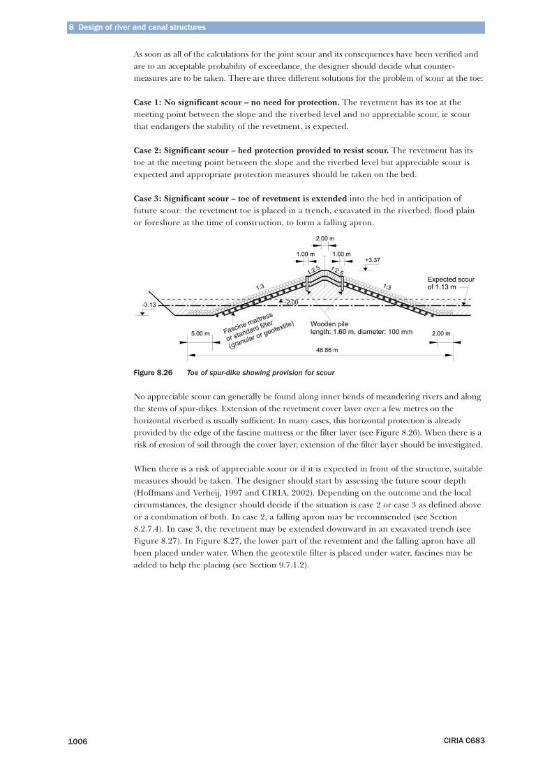
8 Design of river and canal structures
CIRIA C6831006
As soon as all of the calculations for the joint scour and its consequences have been verified andare to an acceptable probability of exceedance, the designer should decide what counter-measures are to be taken. There are three different solutions for the problem of scour at the toe:
Case 1: No significant scour – no need for protection. The revetment has its toe at themeeting point between the slope and the riverbed level and no appreciable scour, ie scourthat endangers the stability of the revetment, is expected.
Case 2: Significant scour – bed protection provided to resist scour. The revetment has itstoe at the meeting point between the slope and the riverbed level but appreciable scour isexpected and appropriate protection measures should be taken on the bed.
Case 3: Significant scour – toe of revetment is extended into the bed in anticipation offuture scour: the revetment toe is placed in a trench, excavated in the riverbed, flood plainor foreshore at the time of construction, to form a falling apron.
Figure 8.26 Toe of spur-dike showing provision for scour
No appreciable scour can generally be found along inner bends of meandering rivers and alongthe stems of spur-dikes. Extension of the revetment cover layer over a few metres on thehorizontal riverbed is usually sufficient. In many cases, this horizontal protection is alreadyprovided by the edge of the fascine mattress or the filter layer (see Figure 8.26). When there is arisk of erosion of soil through the cover layer, extension of the filter layer should be investigated.
When there is a risk of appreciable scour or if it is expected in front of the structure, suitablemeasures should be taken. The designer should start by assessing the future scour depth(Hoffmans and Verheij, 1997 and CIRIA, 2002). Depending on the outcome and the localcircumstances, the designer should decide if the situation is case 2 or case 3 as defined aboveor a combination of both. In case 2, a falling apron may be recommended (see Section8.2.7.4). In case 3, the revetment may be extended downward in an excavated trench (seeFigure 8.27). In Figure 8.27, the lower part of the revetment and the falling apron have allbeen placed under water. When the geotextile filter is placed under water, fascines may beadded to help the placing (see Section 9.7.1.2).
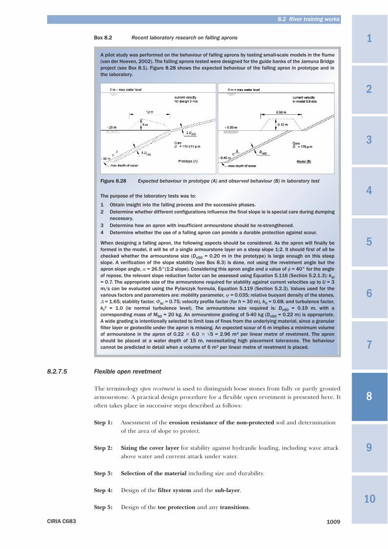
Box 8.2 Recent laboratory research on falling aprons
8.2.7.5 Flexible open revetment
The terminology open revetment is used to distinguish loose stones from fully or partly groutedarmourstone. A practical design procedure for a flexible open revetment is presented here. Itoften takes place in successive steps described as follows:
Step 1: Assessment of the erosion resistance of the non-protected soil and determinationof the area of slope to protect.
Step 2: Sizing the cover layer for stability against hydraulic loading, including wave attackabove water and current attack under water.
Step 3: Selection of the material including size and durability.
Step 4: Design of the filter system and the sub-layer.
Step 5: Design of the toe protection and any transitions.
8.2 River training works
CIRIA C683 1009
A pilot study was performed on the behaviour of falling aprons by testing small-scale models in the flume(van der Hoeven, 2002). The falling aprons tested were designed for the guide banks of the Jamuna Bridgeproject (see Box 8.1). Figure 8.28 shows the expected behaviour of the falling apron in prototype and inthe laboratory.
Figure 8.28 Expected behaviour in prototype (A) and observed behaviour (B) in laboratory test
The purpose of the laboratory tests was to:
1 Obtain insight into the falling process and the successive phases.2 Determine whether different configurations influence the final slope ie is special care during dumping
necessary.3 Determine how an apron with insufficient armourstone should be re-strengthened.4 Determine whether the use of a falling apron can provide a durable protection against scour.
When designing a falling apron, the following aspects should be considered. As the apron will finally beformed in the model, it will be of a single armourstone layer on a steep slope 1:2. It should first of all bechecked whether the armourstone size (Dn50 = 0.20 m in the prototype) is large enough on this steepslope. A verification of the slope stability (see Box 8.3) is done, not using the revetment angle but theapron slope angle, α = 26.5°(1:2 slope). Considering this apron angle and a value of φ = 40° for the angleof repose, the relevant slope reduction factor can be assessed using Equation 5.116 (Section 5.2.1.3): ksl= 0.7. The appropriate size of the armourstone required for stability against current velocities up to U = 3m/s can be evaluated using the Pylarczyk formula, Equation 5.119 (Section 5.2.3). Values used for thevarious factors and parameters are: mobility parameter, ψ = 0.035; relative buoyant density of the stones,Δ = 1.65; stability factor, Φsc = 0.75; velocity profile factor (for h = 30 m), kh = 0.68; and turbulence factor,kt² = 1.0 (ie normal turbulence level). The armourstone size required is: Dn50 = 0.19 m, with acorresponding mass of M50 = 20 kg. An armourstone grading of 5-40 kg (Dn50 = 0.22 m) is appropriate.A wide grading is intentionally selected to limit loss of fines from the underlying material, since a granularfilter layer or geotextile under the apron is missing. An expected scour of 6 m implies a minimum volumeof armourstone in the apron of 0.22 × 6.0 × √5 = 2.96 m³ per linear metre of revetment. The apronshould be placed at a water depth of 15 m, necessitating high placement tolerances. The behaviourcannot be predicted in detail when a volume of 6 m³ per linear metre of revetment is placed.
1
3
4
10
9
8
7
6
5
2
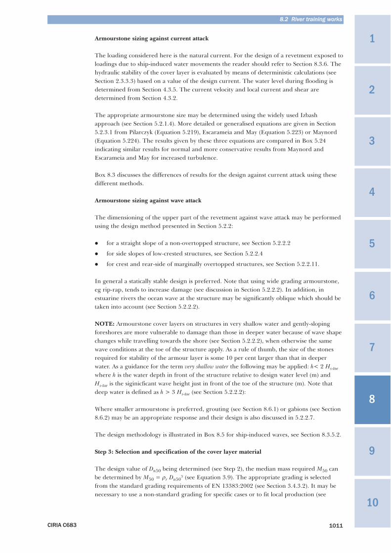
8.2 River training works
CIRIA C683 1011
Armourstone sizing against current attack
The loading considered here is the natural current. For the design of a revetment exposed toloadings due to ship-induced water movements the reader should refer to Section 8.3.6. Thehydraulic stability of the cover layer is evaluated by means of deterministic calculations (seeSection 2.3.3.3) based on a value of the design current. The water level during flooding isdetermined from Section 4.3.5. The current velocity and local current and shear aredetermined from Section 4.3.2.
The appropriate armourstone size may be determined using the widely used Izbashapproach (see Section 5.2.1.4). More detailed or generalised equations are given in Section5.2.3.1 from Pilarczyk (Equation 5.219), Escarameia and May (Equation 5.223) or Maynord(Equation 5.224). The results given by these three equations are compared in Box 5.24indicating similar results for normal and more conservative results from Maynord andEscarameia and May for increased turbulence.
Box 8.3 discusses the differences of results for the design against current attack using thesedifferent methods.
Armourstone sizing against wave attack
The dimensioning of the upper part of the revetment against wave attack may be performedusing the design method presented in Section 5.2.2:
� for a straight slope of a non-overtopped structure, see Section 5.2.2.2
� for side slopes of low-crested structures, see Section 5.2.2.4
� for crest and rear-side of marginally overtopped structures, see Section 5.2.2.11.
In general a statically stable design is preferred. Note that using wide grading armourstone,eg rip-rap, tends to increase damage (see discussion in Section 5.2.2.2). In addition, inestuarine rivers the ocean wave at the structure may be significantly oblique which should betaken into account (see Section 5.2.2.2).
NOTE: Armourstone cover layers on structures in very shallow water and gently-slopingforeshores are more vulnerable to damage than those in deeper water because of wave shapechanges while travelling towards the shore (see Section 5.2.2.2), when otherwise the samewave conditions at the toe of the structure apply. As a rule of thumb, the size of the stonesrequired for stability of the armour layer is some 10 per cent larger than that in deeperwater. As a guidance for the term very shallow water the following may be applied: h< 2 Hs-toewhere h is the water depth in front of the structure relative to design water level (m) and Hs-toe is the siginicficant wave height just in front of the toe of the structure (m). Note thatdeep water is defined as h > 3 Hs-toe (see Section 5.2.2.2):
Where smaller armourstone is preferred, grouting (see Section 8.6.1) or gabions (see Section8.6.2) may be an appropriate response and their design is also discussed in 5.2.2.7.
The design methodology is illustrated in Box 8.5 for ship-induced waves, see Section 8.3.5.2.
Step 3: Selection and specification of the cover layer material
The design value of Dn50 being determined (see Step 2), the median mass required M50 canbe determined by M50 = ρr Dn50³ (see Equation 3.9). The appropriate grading is selectedfrom the standard grading requirements of EN 13383:2002 (see Section 3.4.3.2). It may benecessary to use a non-standard grading for specific cases or to fit local production (see
1
3
4
10
9
8
7
6
5
2
8 Design of river and canal structures
CIRIA C6831012
Section 3.4.3.9). The simple non-standard grading approach is usually sufficient, however, forspecific requirements a detailed approach may be used.
Attention should be paid to durability of the armourstone used (see Section 3.6), notably withreference to weathering processes such as freeze and thaw (see Section 3.8.6).
Box 8.3 Design of a revetment cover layer against current attack
Step 4: Design of the filter system and sublayer
In principle, a granular filter could be used between the subsoil and the cover layer. Inpractice, geotextiles are increasingly used for this purpose. The filter criteria for bothgranular and geotextile filters are given in Section 5.4.3.6. Three different criteria should besatisfied by the filter system:
� functional requirement, ie meeting filter rule requirements
� construction requirement, notably when placing geotextile or granular filter underwater
� durability requirement, ie sufficient resistance during construction and the structurelifetime.
The option of a full multi-layered granular filter, placed in thin layers on a slope underwater,is rarely practicable in river engineering works, except for very large structures. A compositefilter, consisting of a geotextile and a granular layer is more common. Often it is appropriateto place the armour layer directly onto a geotextile (without sublayer), or onto a gravelunderlayer without geotextile.
In Box 8.4, the functional requirements are discussed for the specific case of a geotextilefilter. These functional requirements concern the interface stability of the base soil with thegeotextile filter fabric and the filter permeability. When the cover layer is directly appliedonto the geotextile filter, specific attention should be paid to ensuring it is not damagedduring construction (see Section 9.7.1).
The reader should note that design equations are sensitive to the choice of input parameters. In particular,the depth-averaged velocity should be used for Pilarczyk’s and Maynord’s approaches while the near-bedvelocity is to be used for Escarameia and May’s approach. Standard values of the other input parametersare given in Section 5.2.3.1, however, more detailed values may be relevant. When using Pilarczyk’sapproach, the reader should refer to:
� Section 5.2.1.3 to determine the turbulence factor kt. At a site where fairly high but not excessiveturbulence is expected, a value of r = 0.20 may be used (see Section 4.3.2.5).
� Section 5.2.1.8 to determine the depth factor Λh required to determine the velocity profile factor kh.
When using Escarameia and May’s approach, the reader should refer to Section 4.3.2.5 to determine theturbulence intensity required for calculation of the turbulence coefficient CT.
The result is expressed as an armourstone size required for stability, including a safety coefficient forMaynord’s approach. The reader should note that both Pilarczyk’s and Escarameia and May’s approachesprovide a median size Dn50 that can be easily converted into M50 and allow selection of a standard grading(see Step 3). However, Maynord’s equation provides a median sieve size D50 with Dn50 ≅ 0.84 D50 (seeSection 3.4.2 for further discussion on the relation between Dn and D).
A standard double layer thickness is 2kt Dn50 (see Section 3.5.1 for values of the layer thicknesscoefficient, kt (-)). When small armourstone is required for weak currents, it may be practical to use athicker layer to sink a geotextile and a fascine mattress. Conversely, assuming a minimum thickness of0.5 m is required for construction purposes, ie Dn50 = 0.203 m, the hydraulic stability for this armourstonesize may be checked to confirm if sufficient.
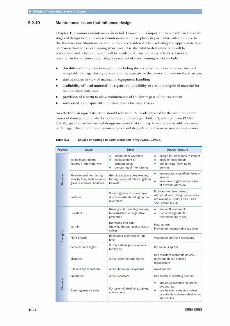
8 Design of river and canal structures
CIRIA C6831024
8.2.10 Maintenance issues that influence design
Chapter 10 examines maintenance in detail. However, it is important to consider in the earlystages of design how and when maintenance will take place, in particular with reference tothe flood season. Maintenance should also be considered when selecting the appropriate typeof cross-section for river training structures. It is also vital to determine who will beresponsible and what equipment will be available for maintenance activities. Issues toconsider in the various design stages in respect of river training works include:
� durability of the protection system, including the accepted reduction in stone size andacceptable damage during service, and the capacity of the owner to maintain the structure
� size of stones in view of manual or equipment handling
� availability of local material for repair and possibility to create stockpile of material formaintenance purposes
� provision of a berm to allow maintenance of the lower part of the revetment
� wide crest, eg of spur-dike, to allow access for large trucks.
An effectively designed structure should withstand the loads imposed by the river, but othercauses of damage should also be considered in the design. Table 8.3, adapted from PIANC(1987b), gives an aide-memoire of design measures that can help to overcome or address causesof damage. The aim of these measures is to avoid degradation or to make maintenance easier.
Table 8.3 Causes of damage to bank protection (after PIANC, 1987b)
Feature Cause Effect Design measure
Abra
sion
Ice floes and debrisfloating in the waterway
� impact near waterline� displacement of
armourstones� puncturing of membranes
� design for resistance to impact� allow for easy repair� deflect water flow, eg by
groynes
Abrasive sediment in highvelocity flow, such as sand,gravels, cobbles, boulders
Grinding action at toe wearingthrough exposed fabrics, gabionbaskets
� incorporate a sacrificial layer ofarmour
� avoid use of gabions in casesof extreme abrasion
Pack iceShearing force on cover layerdue to ice-sheets riding up therevetment
Provide cover layer able towithstand load, design proceduresare available CRREL (1980) andsee Section 5.2.4)
Bio
logi
cal
LivestockGrazing and trampling leadingto destruction of vegetativeprotection
� fence-off revetment� use non-degradable
reinforcement to soil
VerminBurrowing into bankGnawing through geotextiles orcables
Pest controlProvide an impenetrable top layer
Plant growthRoots alter geometry of toplayer
Vegetation control if necessary
Seaweed and algaeSurface damage to asphaltictop layers
Bituminous sprays
Microbes Attack some natural fibresUse resistant materials unlessdegradation is a specificrequirement
Chem
ical
Oils and hydro-carbons Attack bituminous systems Avoid contact
Sulphates Attack concrete Use sulphate resisting cement
Other aggressive saltsCorrosion of steel wire, cables,connections
� protect by galvanising and/orpvc coating
� use heavier wires and cables,or suitable stainless steel wiresand cables
8 Design of river and canal structures
CIRIA C6831064
8.7 REFERENCES
BAW (Bundesanstalt für Wasserbau) (1990). Code of practice – Use of Cement-bonded andBitumen-bonded materials for grouting armourstone on Waterways. MAV, Karlsruhe, Bundesandtaltfur Wasserbau
Bonasoundas, M (1973). Stromungsvorgang und Kolkproblem am runden Brückenpfeiler [Flowstructure and problems at circular bridge piers]. PhD thesis / Report no. 28, Oskar V. MillerInstitute, Technical University, Munich [in German]
CRREL [Cold Regions Research and Engineering Laboratory] (1980) IAHR Working group onice forces on structures. Carstens, T. Special report 80-26, June, 153 pp
CUR/TAW (1991). Guide for the design of riverdikes volume 1 – upper river area. CUR, Gouda, pp59-65
Delft Hydraulics (1973). Improvement of the navigability of the river-canal crossing near Wijk bijDuurstede, The Netherlands; morphological aspects. Delft Hydraulics report M974-975 (in Dutch)
Delft University (1983). Hydraulic response to wind and ship induced waves for channel and coastaldesign, Delft University Press, Delft
Environment Agency (1999). Waterway bank protection: a guide to erosion assessment andmanagement. R&D Publication 11, The Stationary Office, pp105
Escarameia, M (1998). Design manual on river and channel revetments. Thomas Telford, London
Hemphill, R W and Bramley, M E (1989). Protection of river and canal banks. CIRIA report,Butterworths, London
Hjorth, P (1975). Studies on the nature of local scour. Bulletin Series A, No. 46, 1975. Dept.Water Resources Engineering, Lund Institute of Technology, University of Lund, Sweden
Hoffmans, G J C M and Verheij, H C (1997). Scour manual. AA Balkema, Rotterdam, TheNetherlands, 205 pp, ISBN 9054106735
Jansen, P, Ph, Van Bendegom, L, Van Den Berg, M, De Vries, M and Zanen, A (1994).Principles of river engineering; The non-tidal alluvial river. Pitman, London, ISBN: 9040712808
Larinier, M, Porcher, J P, Travade, F and Gosset, C (1994). Passes à poisons, expertise,conceptiondes ouvrages de franchissement collection mise au point. Conseil Supérieur de la Pêche, 336 pp
LCPC (1989). Les enrochements. Ministère de l'Equipement, Paris, 106 pp
Mamak, D W (1958). River regulation. (translated and re-print of publication in Polish), Officeof Technical Services, US Dep of Commerce, Washington
May, R, Ackers, J and Kirby, A (2002). Manual on scour at bridges and other hydraulic structures.CIRIA, C551, London
McDonald, G N (1988). “Riprap and armour stone”. In: A C T Chen and C B Leidersdorf(eds), Arctic coastal processes and slope protection design: a state of the practice report. TechnicalCouncil on Cold Regions Engineering Monograph, ASCE, New York, pp 190–207
PIANC (1987a). Guidelines for the design and construction of flexible revetments incorporatinggeotextiles for inland waterways. InCom Working Group 04, Supplement to PIANC Bulletin No57, Brussels
PIANC (1987b). Risk consideration when determining bank protection requirements. InCom WorkingGroup 03, Supplement to PIANC Bulletin No 58, Brussels
Pilarczyk, K W (1998). Dikes and revetments: design, maintenance and safety assessment. AA Balkema,Rotterdam
Rajaratnam, N (1976). Turbulent jets. Elsevier Scientific Publishing Company, Amsterdam andNew York, 304 pp
Simons, D B (1984). Hydraulic test to develop design criteria for the use of reno mattresses. WaterResources Archive, Colorado State University, Fort Collins
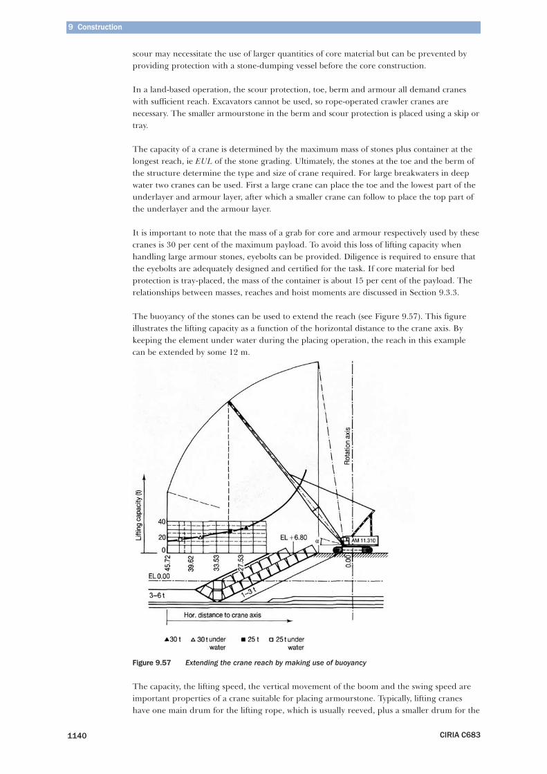
9 Construction
CIRIA C6831140
scour may necessitate the use of larger quantities of core material but can be prevented byproviding protection with a stone-dumping vessel before the core construction.
In a land-based operation, the scour protection, toe, berm and armour all demand craneswith sufficient reach. Excavators cannot be used, so rope-operated crawler cranes arenecessary. The smaller armourstone in the berm and scour protection is placed using a skip ortray.
The capacity of a crane is determined by the maximum mass of stones plus container at thelongest reach, ie EUL of the stone grading. Ultimately, the stones at the toe and the berm ofthe structure determine the type and size of crane required. For large breakwaters in deepwater two cranes can be used. First a large crane can place the toe and the lowest part of theunderlayer and armour layer, after which a smaller crane can follow to place the top part ofthe underlayer and the armour layer.
It is important to note that the mass of a grab for core and armour respectively used by thesecranes is 30 per cent of the maximum payload. To avoid this loss of lifting capacity whenhandling large armour stones, eyebolts can be provided. Diligence is required to ensure thatthe eyebolts are adequately designed and certified for the task. If core material for bedprotection is tray-placed, the mass of the container is about 15 per cent of the payload. Therelationships between masses, reaches and hoist moments are discussed in Section 9.3.3.
The buoyancy of the stones can be used to extend the reach (see Figure 9.57). This figureillustrates the lifting capacity as a function of the horizontal distance to the crane axis. Bykeeping the element under water during the placing operation, the reach in this examplecan be extended by some 12 m.
Figure 9.57 Extending the crane reach by making use of buoyancy
The capacity, the lifting speed, the vertical movement of the boom and the swing speed areimportant properties of a crane suitable for placing armourstone. Typically, lifting craneshave one main drum for the lifting rope, which is usually reeved, plus a smaller drum for the
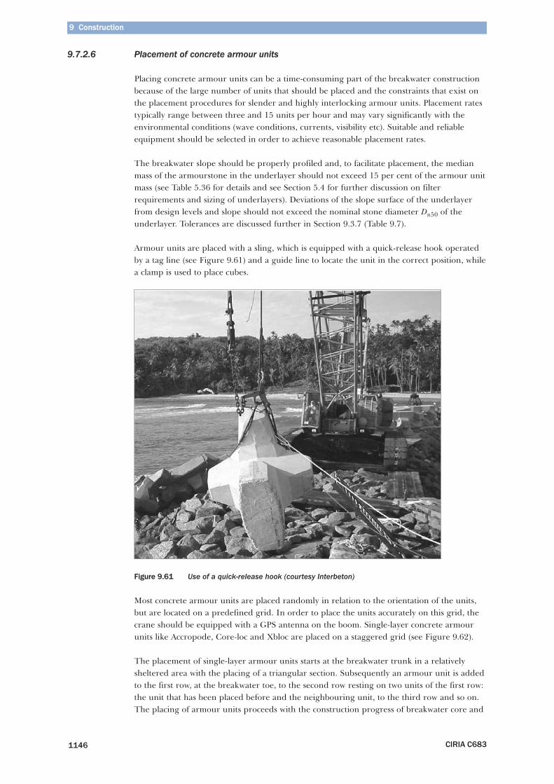
9 Construction
CIRIA C6831146
9.7.2.6 Placement of concrete armour units
Placing concrete armour units can be a time-consuming part of the breakwater constructionbecause of the large number of units that should be placed and the constraints that exist onthe placement procedures for slender and highly interlocking armour units. Placement ratestypically range between three and 15 units per hour and may vary significantly with theenvironmental conditions (wave conditions, currents, visibility etc). Suitable and reliableequipment should be selected in order to achieve reasonable placement rates.
The breakwater slope should be properly profiled and, to facilitate placement, the medianmass of the armourstone in the underlayer should not exceed 15 per cent of the armour unitmass (see Table 5.36 for details and see Section 5.4 for further discussion on filterrequirements and sizing of underlayers). Deviations of the slope surface of the underlayerfrom design levels and slope should not exceed the nominal stone diameter Dn50 of theunderlayer. Tolerances are discussed further in Section 9.3.7 (Table 9.7).
Armour units are placed with a sling, which is equipped with a quick-release hook operatedby a tag line (see Figure 9.61) and a guide line to locate the unit in the correct position, whilea clamp is used to place cubes.
Figure 9.61 Use of a quick-release hook (courtesy Interbeton)
Most concrete armour units are placed randomly in relation to the orientation of the units,but are located on a predefined grid. In order to place the units accurately on this grid, thecrane should be equipped with a GPS antenna on the boom. Single-layer concrete armourunits like Accropode, Core-loc and Xbloc are placed on a staggered grid (see Figure 9.62).
The placement of single-layer armour units starts at the breakwater trunk in a relativelysheltered area with the placing of a triangular section. Subsequently an armour unit is addedto the first row, at the breakwater toe, to the second row resting on two units of the first row:the unit that has been placed before and the neighbouring unit, to the third row and so on.The placing of armour units proceeds with the construction progress of breakwater core and
9.8 Quality control
CIRIA C683 1163
It has been stressed that in the design process new guidance on layer thickness and as-placeddensity, especially of individually placed armour layers, as presented in Section 3.5.1, shouldbe adopted in finalising design profiles. The mass of armourstone that the contractor haspurchased and placed in the armour layer is then more likely to be close to the designer’sestimate of required mass calculated from the design volume. The designer or client requiresquality workmanship without liability for paying for fluids when rock was wanted, andwithout liability for paying for overly tight armourstone when less material was intended.The contractor wants speedy execution and full recouping of the cost outlay on materials. Itis important to recognise a balance between the two parties’ legitimate concerns. Thisrequires that the designer’s assumption for the armour layer porosity, nv , applicable to thespherical probe survey method, is known, and that the validity of this assumption is checkedduring approval of the test panel.
It is recommended that the client declares in the contract:
� the payment rate for the mass of armourstone placed in each class of armourstone
� the assumed armour layer porosity, nv , in each class of armourstone
� the assumed design layer thickness coefficient, kt, for armour layers.
The test panel should form part of a larger completed section within realistic boundaries.Blocks falling on the boundaries of the panel are treated appropriately so as not to biasresults. Particular care should be taken to ensure the test panel armourstone is representativeof the specified grading. If necessary, adjustments to the trial panel are made until:
� grading is within specification
� final survey heights are within tolerance limits of the design drawing heights. Anyserious difficulty in meeting these tolerances suggests that stone shape characteristicshave not been accounted for and/or that inappropriate estimates of the kt factor wereassumed in the design. These problems can be resolved by rebuilding, resetting thedesign drawing surface levels or resetting tolerances
� in the eyes of the engineer, the visual appearance reflects the designer’s intention asimplied by the placement methods referred to in the contract and classified as random,standard, dense or specific.
This trial panel is then termed visually accepted and is subject to further analysis.
Given the placement method referred to in the contract on the one hand, and the blend ofon-site factors (materials characteristics, placement machinery, operator training andexperience, working conditions, time constraints) on the other, the trial panel exercise maypoint to a need to revise the most appropriate layer (or volumetric) porosity assumption foruse in the payment calculation if payment is on a basis of armourstone tonnages deducedfrom surveyed volumes and target layer porosity.
Data obtained from the visually accepted test panel include:
� individual masses of all blocks in the panel. This provides further on-site control ofheavy gradings. Individual weighing is preferred to the alternative of mass estimationfrom density and volume assessment using suitable block dimensions and shape factors.The total mass of armour in the panel is divided by apparent rock density, ρapp (kg/m3),to give the volume of armourstone in the panel, Vr (m3)
� the surveyed armour layer volume, Vbs , corrected to spherical end 0.5Dn50 probemethod. The chainage length is multiplied by the average area enclosed between theupper and lower surveyed surface of the armour layer (see Equation 3.24, Vbs = AcsL).Normally it should be sufficient to have four profile lines surveyed across the structure at2.5 m intervals, making sure the end points of the survey line are included
1
3
4
10
9
8
7
6
5
2
9 Construction
CIRIA C6831164
� the number of blocks placed in the armour layer per unit of slope area covered. Thisshould be presented both for the visible upper layer of blocks and for the total numberof blocks.
Equation 9.9 gives the relation between the armour layer porosity (expressed as a fraction) ofthe visually accepted test panel and the relevant armour layer volumes.
(9.9)
If there is less than a 2 per cent difference in value between nvp and nv assumed in the design(ideally also indicated in the contract), the panel is in every way acceptable as a constructionbenchmark to be followed for the contract.
If the difference is more than 2 per cent, another attempt might be made to construct nearerto the design armour layer porosity, without an unreasonably onerous burden being placedon the rate of build, given the classified placement method originally specified.
If after this rebuild the new surfaces surveyed fulfil tolerances and are visually accepted, butthe test panel still has more than a 2 per cent difference, the contractor and engineer shouldagree that this panel becomes the benchmark for acceptable construction practices.
For those contracts where payment is based on a tonnage placed calculated from volumesurveys, it is also an opportunity to validate and if necessary, revise the armour layer porosityassumption. If the contract states a pay rate for tonnage of armourstone placed in the worksto be a tonnage calculated from surveyed bulk volume, assumed armour layer porosity andapparent rock density, then an appropriate basis for payment of the panel (see Equation 3.26,Vr = Vb (1 - nv)) is given by Equation 9.10, an expression for the total mass of the armour, Mt .
(9.10)
Placement workmanship at sample areas throughout the structure may be compared with thetest panel(s) on visual criteria and also by comparing the number of blocks per unit area withresults from the test panel(s). Major variations in block count results should be explained andremoved by reworking if necessary. As the finished profiles of the entire works are normallychecked for tolerances, the bulk-placed volumes of the entire armour layer in the completedstructure can be similarly computed and bills for placed tonnages prepared accordingly.Precisely worded clauses usually exist to exclude liability for the client having to pay forarmourstone determined by survey to be on average above an upper tolerance line.
Alternative simple schemes for payment based directly on tonnages placed exist. Forexample, contract payment for armour materials may be based on a rate per tonne deliveredto site given satisfactory criteria for proof of delivery to site.
9.9 SURVEY AND MEASUREMENT TECHNIQUES
Because of the direct relationship between survey techniques and payments, all parties to aworks contract should ensure that an accurate, fair and pragmatic approach to surveying isadopted that will lead to the correct method of payment for the work done. To suit therequirements of the works, tolerance levels should be practical, sensible, achievable andaffordable. The various definitions of the term tolerance are set out in Section 9.3.7.
In addition to discussing the various survey techniques, this section also provides tables withinformation on achievable vertical tolerances for land-based and marine equipment, for bothbulk and individually placed armourstone and concrete armour units.
n V Vvp r bs= −( )1
M V nt app bs vp= ⋅ −( )ρ 1
The Rock Manual
CIRIA C683xxviii
Ds Size of the equivalent volume sphere (m)Dz Block size corresponding to sieve size z (m)D50 Sieve diameter, diameter of stone that exceeds the 50% value of sieve curve (m)D85 85% value of sieve curve (m)D15 15% value of sieve curve (m)D63.2 Location parameter in the Rosin-Rammler equation for sieve size distribution (m)D* Non-dimensional sediment grain diameter, D* = D50(gΔ /ν²)1/3 (-)d Structure (crest) height relative to bed level (breakwaters, dams etc) (m)d Thickness or minimum axial breadth (given by the minimum distance between
two parallel straight lines between which an armour block can just pass) (m)dc Crown wall height (m)dca Difference of level between crown wall and armour crest, dca = Rc - Rca (m)E Young’s Modulus (N/m²)E Estuary number (-)Ec Impact energy absorbance capacity (kNm)ED Total degradation energy applied to the material (J)Ei Incident wave energy (N/m)Er Reflected wave energy (N/m)Et Transmitted wave energy (N/m)Eηη Energy density of a wave spectrum (m²s)Ei;d Design value of the effect of actions (Unit of E)Ei;k Characteristic value of the effect of actions (Unit of E)e Void ratio, e = nv /(1 - nv) (-)esp Spur ratio, defined as the ratio of the head loss in a river between two
successive spur-dikes, U²Ssp/(C²h), and the velocity head, U²/(2g) (m)F Fetch length (m)F Factor of safety (geotechnical), defined as ultimate resistance/required resistance (-)F* Non-dimensional freeboard parameter, F*= (Rc /Hs)² (som/2π) (-)Fr Froude number, Fr = U/(gh)1/2 (-)FH Horizontal force (on caisson or crown wall element) (N/m)FU Uplift force (on caisson or crown wall element) (N/m)Fj;d Design value of an action or force (N/m)Fj;k Characteristic value of an action or force (N/m)Fq Discharge factor, ratio of critical discharge for bed protection and that of
closure dam, qcr-b / qcr-d (-)Fo Parameter expressing the amount of fines after minor breakage (%)Fs Shape factor (of armour stone) (-)f Friction factor (-)f Frequency of waves, f = 1/T (1/s)f Lacey’s silt factor (-)fc Friction factor for currents (-)fi Stability increase factor for armourlayers with stepped or bermed slopes (-)fp Peak frequency of wave spectrum (1/s)fw Friction factor for waves (-)G Shear modulus (N/m²)g Gravitational acceleration (m/s²)H Wave height, from trough to crest (m)H Water level upstream of a dam or sill, relative to dam crest (m)H1/10 Mean height of highest 1/10 fraction of waves (m)H1/3 Significant wave height based on time domain analysis, average of highest
1/3 of all wave heights (m)H2% Wave height exceeded by 2% of waves (m)Ho Stability number, Ho = Ns = Hs /(ΔDn50) (-)HoTo Dynamic stability number, HoTo = Nsd = NsTm(g/Dn50)1/2 (-)Hd Drop height (m)