BsÆ J/Ψφ Æ J/Ψ System (A Short Summary)

NEPPSR, 2004 Colin Gay, Yale University

Time Dependent Angular Analysis ofBs J/Ψφ and Bd J/ΨK* decays, and aLifetime Difference in the Bs System

(A Short Summary)

Ke Li, C. Gay, M. Schmidt (Yale)Konstantin Anikeev, C. Paus (MIT)

For the CDF II Collaboration

Colin Gay, Yale University


Overview

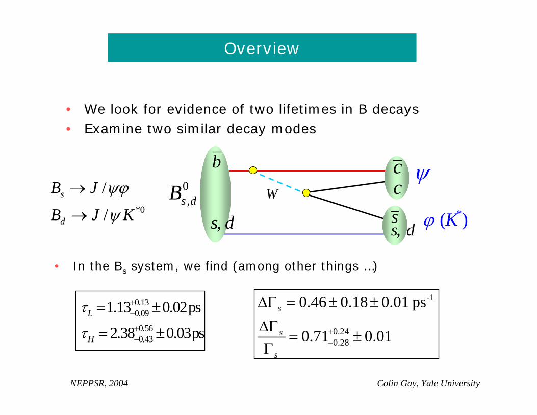
• We look for evidence of two lifetimes in B decays• Examine two similar decay modes

*0

/

/s

d

B J

B J K

ψϕ

ψ

→

→

ψ

*( )Kϕ

0,s dB

ccs,s d,s d

b

-1

0.240.28

0.46 0.18 0.01 ps

0.71 0.01

s

s

s

+−

∆Γ = ± ±

∆Γ= ±

Γ

0.130.09

0.560.43

1.13 0.02ps

2.38 0.03psL

H

τ

τ

+−

+−

= ±

= ±

• In the Bs system, we find (among other things …)

W


Unitarity Triangle

(ρ,η)

(1,0)(0,0)

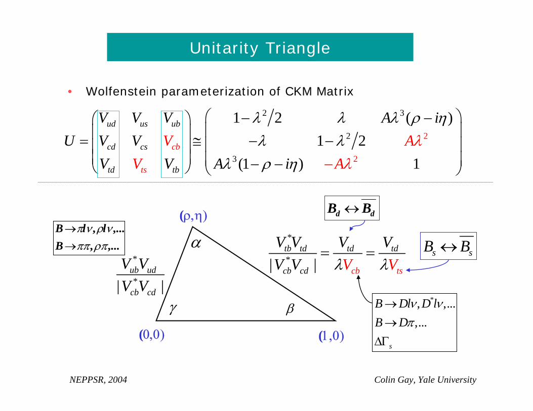
dd BB ↔

,...,,...,

ρπππνρνπ

→→

BllB

*, ,...,...

s

B Dl D lB D

ν νπ

→→

∆Γ

*

*| |tb td td td

cb c b tsd c

V V VV V

VV V λ λ

= =*

*| |ub ud

cb cd

V VV V

s sB B↔α

βγ

2

23

2

3

2

1 2 ( )1 2

(1 ) 1cb

ts

ud us ub

cd cs

td tb

V V V A iU V V

V VV A

V AA i

λ λ λ ρ ηλ λ

λ ρλ

λη

⎛ ⎞− −⎛ ⎞⎜ ⎟⎜ ⎟= ≅ − −⎜ ⎟⎜ ⎟

⎜ ⎟ ⎜ ⎟− −⎝ ⎠ ⎝ ⎠−

• Wolfenstein parameterization of CKM Matrix


B Oscillations

12 12* *12 122

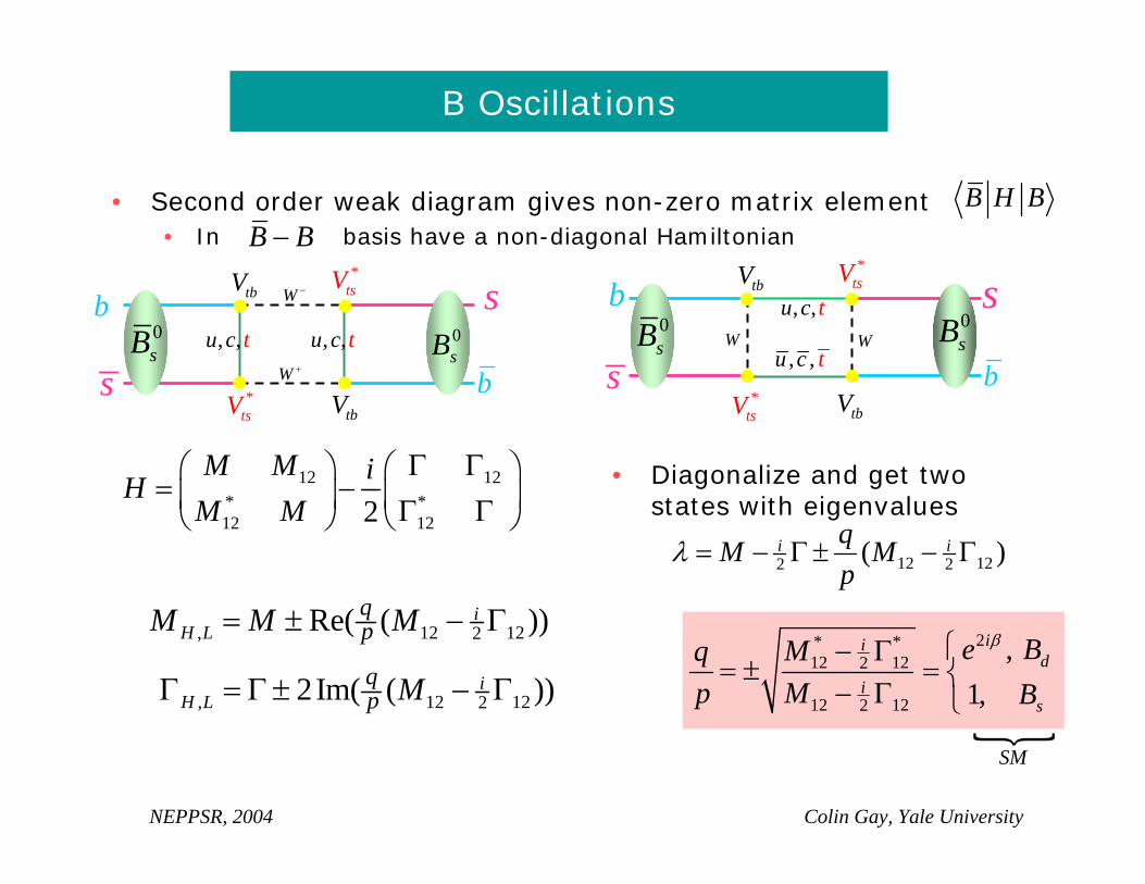
M M iHM M

Γ Γ⎛ ⎞ ⎛ ⎞= −⎜ ⎟ ⎜ ⎟Γ Γ⎝ ⎠ ⎝ ⎠

• Second order weak diagram gives non-zero matrix element• In basis have a non-diagonal Hamiltonian

B H BB B−

• Diagonalize and get two states with eigenvalues

b s

bs0sB 0

sB, ,u c t , ,u c t

*tsV

tbV

tbV

*tsV

W +

W − b s

bs0sB 0

sB, ,u c t

, ,u c t*

tsV

tbV

tbV

*tsV

W W

2* *12 122

12 122

,1,

iid

is

e BMqp M B

β⎧− Γ= ± = ⎨− Γ ⎩

12 122 2( )i iqM Mp

λ = − Γ ± − Γ

, 12 1222Im( ( ))iH L

qp MΓ = Γ ± − Γ

, 12 122Re( ( ))iH L

qpM M M= ± − Γ

SM


Eigenstates

12

12

| | |

|

(| | )

| )| | ( |

Hs s s s

ss s

s

Ls s

B B

B B

B p B q B

B p B q B

⟩ = ⟩ + ⟩ =

⟩

⟩+ ⟩

⟩−= ⟩ − = ⟩⟩

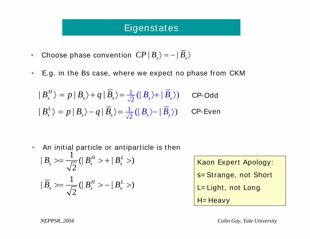
| |s sCP B B⟩ = − ⟩• Choose phase convention

1| (| | )2

1| (| | )2

H Ls s s

H Ls s s

B B B

B B B

>= > + >

>= > − >

• E.g. in the Bs case, where we expect no phase from CKM

CP-Odd

CP-Even

• An initial particle or antiparticle is then

Kaon Expert Apology:

s=Strange, not Short

L=Light, not Long

H=Heavy


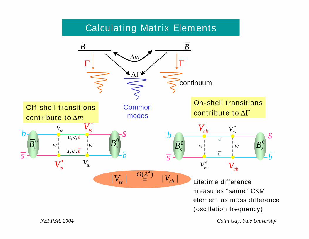
Calculating Matrix Elements

Commonmodes

m∆

∆Γ

B B

continuum

ΓΓ

b s

bs0sB 0

sB, ,u c t

, ,u c t

*tsV

tbV

tbV

*tsV

W W

On-shell transitionscontribute to

Off-shell transitionscontribute to

*csV

cbV

b s

bs0sB 0

sBc

c

cbV *csV

W W

| |tsV | |cbV=

m∆ ∆Γ

Lifetime differencemeasures “same” CKM element as mass difference(oscillation frequency)

4( )O λ


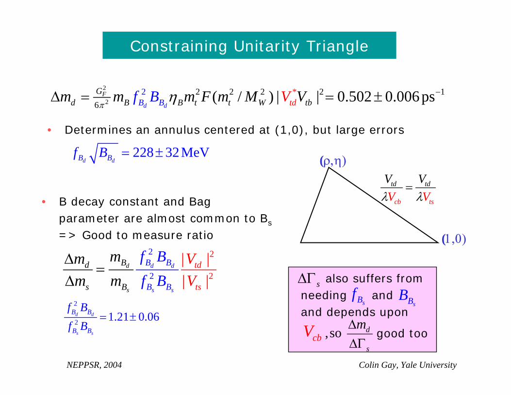
Constraining Unitarity Triangle

2

22 2 2 2 1

6*2 ( / ) | | 0.502 0.006 psF

d d

Gd B B t t W tbdB tBm m m F m Mf B VV

πη −∆ = = ±

2

2

2

2

| || |

d dd

ss s

Bd B B

B

t

s B

d

tsB

f Bf B

VV

mmm m

∆=

∆2

2 1.21 0.06d d

s s

B B

B B

f Bf B

= ±

228 32MeVd dB Bf B = ±

• Determines an annulus centered at (1,0), but large errors

• B decay constant and Bagparameter are almost common to Bs

=> Good to measure ratio

(ρ,η)

(1,0)

td t

t

d

cb s

V VV Vλ λ

=

s∆Γ also suffers fromneeding andand depends upon

sBf sBB

cbV ,so d

s

m∆∆Γ

good too


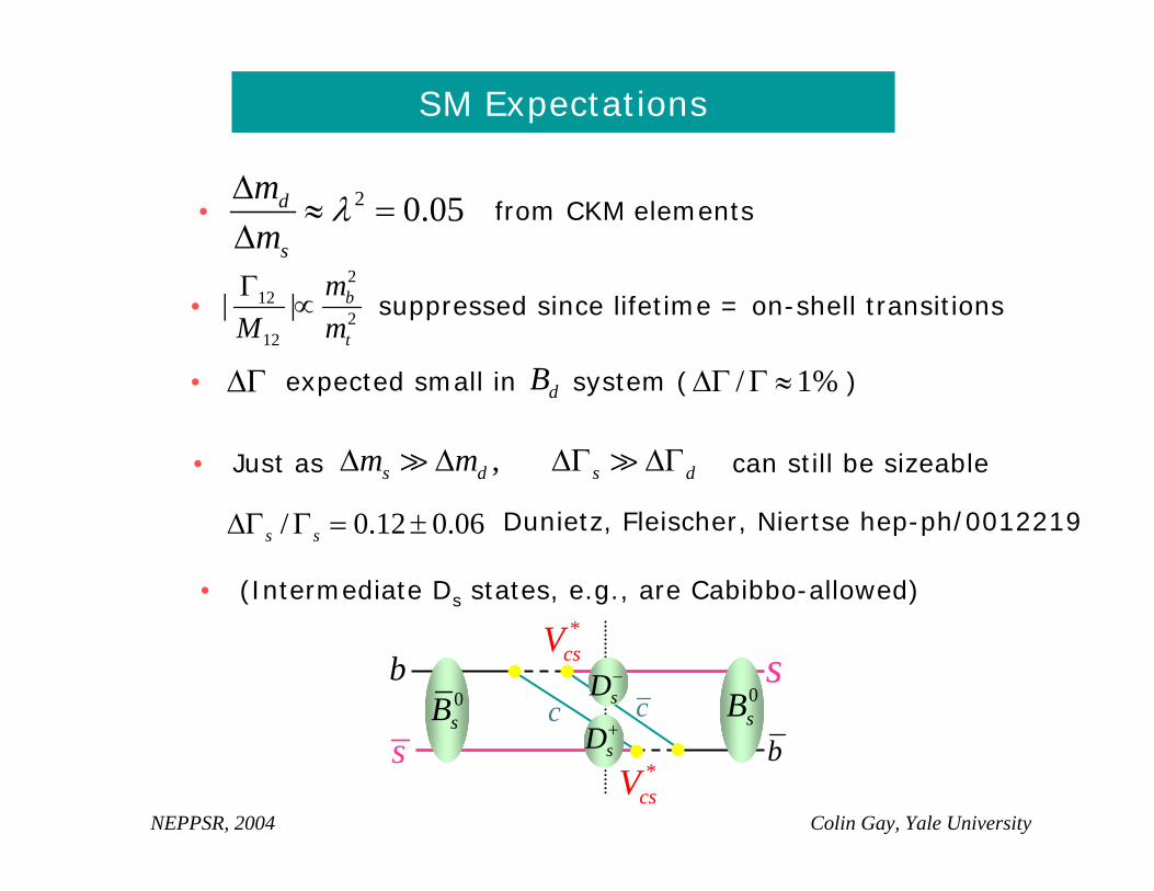
SM Expectations

∆Γ

2 0.05d

s

mm

λ∆≈ =

∆from CKM elements

• suppressed since lifetime = on-shell transitions

• expected small in system ( )

212

212

| | b

t

mM mΓ

∝

dB / 1%∆Γ Γ ≈

• Just as can still be sizeable ,s d s dm m∆ ∆ ∆Γ ∆Γ

/ 0.12 0.06s s∆Γ Γ = ±

•

b s

bs

sD−

sD+c c 0

sB0sB

*csV

*csV

Dunietz, Fleischer, Niertse hep-ph/0012219

• (Intermediate Ds states, e.g., are Cabibbo-allowed)


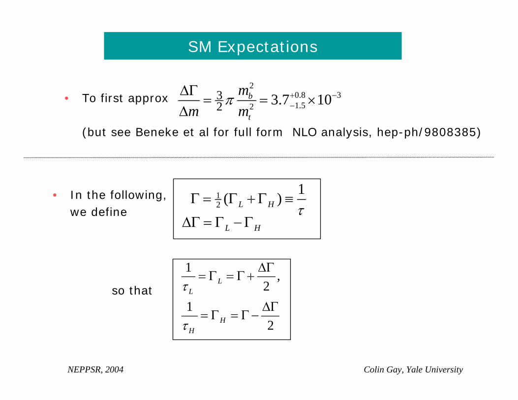
SM Expectations

• To first approx

(but see Beneke et al for full form NLO analysis, hep-ph/9808385)

12

1( )L H τΓ = Γ + Γ ≡

L H∆Γ = Γ − Γ

• In the following,we define

20.8 31.52

32 3.7 10b

t

mm m

π + −−

∆Γ= = ×

∆

1 ,2

12

LL

HH

τ

τ

∆Γ= Γ = Γ +

∆Γ= Γ = Γ −

so that


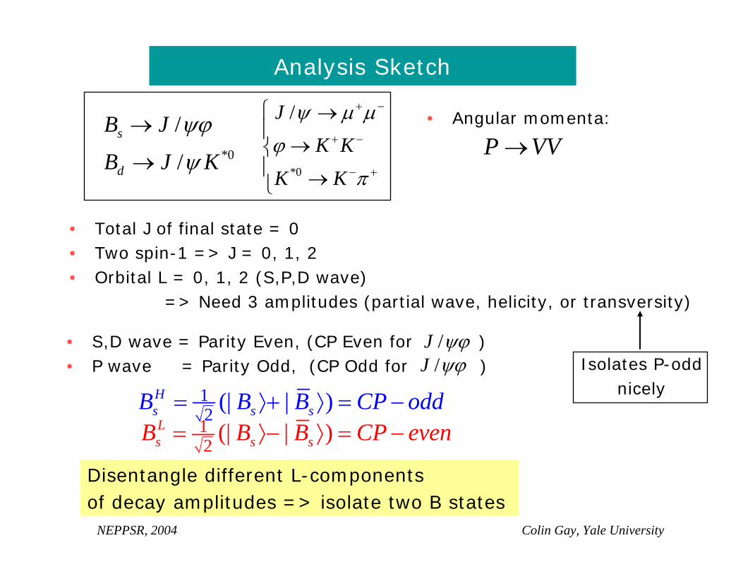
Analysis Sketch

P VV→

• Total J of final state = 0• Two spin-1 => J = 0, 1, 2• Orbital L = 0, 1, 2 (S,P,D wave)

=> Need 3 amplitudes (partial wave, helicity, or transversity)

• S,D wave = Parity Even, (CP Even for )• P wave = Parity Odd, (CP Odd for )

12 (| | )H

s s sB B B CP odd= ⟩+ ⟩ = −12 (| | )L

s s sB B B CP even= ⟩− ⟩ = −

Disentangle different L-componentsof decay amplitudes => isolate two B states

*0

/

/s

d

B J

B J K

ψϕ

ψ

→

→

/J ψϕ

*0

/JK K

K K

ψ µ µ

ϕ

π

+ −

+ −

− +

⎧ →⎪

→⎨⎪ →⎩

/J ψϕ

• Angular momenta:

Isolates P-oddnicely


Transversity Angles

Θ

Φ

z

y

xK +

K −ϕ

µ +

µ −

KK plane defines (x,y) planeK+(K) defines +y direction

Θ, Φ polar & azimuthal angles of µ+Ψ helicity angle of φ (Κ∗)

• Work in J/Ψ rest Frame


Decay Angular Distributions

0 longitudinal pol. amplitudetransverse pol. ampli e, tud s

AA A⊥

=

=


Fit Functions

• UNTAGGED analysis•Don’t try to tell if initial state is orB B

evenodd

L

H

CPCP=

Γ =−Γ−


Decay Modes

ψφJ/→SB

µ+ µ-

K+

J/ψφ

<L>~

1 mm

σx ~ σy~20 µm

B S

PV

SV

µ+ µ-K+

π-

<L>~

1 mm

B d

SV

J/ψ

K*0

σx ~ σy~20 µmPV

*J/ KBd ψ→

σL~30 µm

Compare the two similar topologies

K-

σL~30 µm


Sample Selection

• Track Selection• PT > 0.4 GeV• Well-measured in

Central Tracker• All 4 tracks have

Silicon Detector hits• J/Ψ Selection

• PT > 1.5 GeV• Mass within 80 MeV of

PDG • J/Ψ trigger path

(unbiased in lifetime)

• Momenta (PT) • K* > 2.6 GeV,

Bd > 6.0 GeV• φ > 2.0 GeV,

Bs > 6.0 GeV

• Mass windows

• φ : 6.5 MeV• K* : 50 MeV

• Closest Kπ assignment to K*

chosen (=swaps~10 %)• B meson Vertex:

• Constrain J/Ψ mass • Primary vertex from beamline

• ~260 pb-1 taken up to Feb 2004 (start of COT problem–now fixed!!)


Detector Acceptance

• 40 M decays generated flat inangular variables

• Shapes show effect of cutsand detector sculpting

ϕcosθ

cosψ


Mass and Lifetime Projections (Bd)

0 462 15 4B

c mτ µ= ± ±460.8 4.2PDG mµ= ±

.01d

d

∆Γ≤

Γis small in SM=>Fit to 1 lifetime


B+ Lifetime

-11.660 0.033 psuτ = ±

~ 3300N

-11.671 0.018 psuτ = ±PDG:

CDF Run II:


Angular Projections (Bd)

• Sideband subtracted,acceptance corrected projections

• Full Likelihood Fit is simultaneousin angular variables

• Can’t see correlations in these projections


Bd Amplitudes vs. BaBar/Belle


Bs Results

• Perform two fits1. Unconstrained: Fit data as described

2. Constrained: Invoke SM constraint(Expected true to ~1%)

Sinceset

12 ( )s H L dΓ = Γ + Γ = Γ

1.54 0.014psdτ = ±

21 1.54 0.021psL H

s L H

τ ττ τ

= = ±Γ +


Mass and Lifetime Projections (Bs)— Unconstrained Fit

0.160.13

0.580.46

1.05 0.02ps

2.07 0.03psL

H

τ

τ

+−

+−

= ±

= ±

0.19 -10.24

0.250.33

0.47 0.01 ps

0.65 0.01

s

s

s

+−

+−

∆Γ = ±∆Γ

= ±Γ

CP-odd fraction ( ) ~ 22%Hτ


Lifetime Projection (Bs)— Constrained Fit

• SM Predictsto ~1%

: constrain in fit s dΓ = Γ

-1

0.240.28

0.46 0.18 .01 ps

0.71 0.01

s

s

s

+−

∆Γ = ± ±

∆Γ= ±

Γ

0.130.09

0.560.43

1.13 0.02ps

2.38 0.03psL

H

τ

τ

+−

+−

= ±

= ±

• Remember,can’t see angularseparation of CPeigenstates inprojection


Main Fitting resultsAny

two a

t a

tim

e

⎧⎨⎩


Systematics

• Alignment• Lifetime Fit model• Procedure Bias• Cross-feed• Detector Acceptance• Monte Carlo - data matching• K-π swap• Non-resonant decays• Background angular model• Unequal amounts of

⎫⎬⎭

From high-statisticsstudiesand J/B ψ+

B B−


Systematics


Cross Check: Bd Fit

• Bd sample is ~4 times as large as Bs•Fit Bd sample with Bs fit function•Split sample into 4 subsamples of size ~ Bs sample size

• Note: This is not a measurement of /d d∆Γ Γ


Cross Check: Bs and Bd CP odd fraction

• Fit to amplitudes ONLY, using different minimum lifetime cuts.

• Clear CP odd fraction increase suggests relative large lifetime difference on the two components

• Angular distribution is saying the same thing as the lifetime information

Predicted (%)Fitted (%)Cut (µm)

33.638.7 ± 11.6>450

28.629.6 ± 12.7>300

24.124.2 ± 10.3>150

--20.1--20.1 ± 9.0>0

Fitted (%)Cut (µm)

23.6 ± 4.9>450

23.0 ± 4.0>300

23.0 ± 3.6>150

21.6 ± 4.4>0

Bd CP-odd fraction

Bs CP-odd fractionExp

ect constan

t


Prob(0), Prob(SM)

Input ∆Γ/Γ = 0• Unconstrained Fit

• 1/315 give ∆Γ/Γ > 0.65

• Constrained Fit• 1/718 give ∆Γ/Γ > 0.71

Input ∆Γ/Γ = 0.12 (SM prediction)• Unconstrained Fit

• 1/84 give ∆Γ/Γ > 0.65

• Constrained Fit• 1/204 give ∆Γ/Γ > 0.71

• Note: These answer the question:•If true value = X, what is the chance to see our measurement

• Not the same as asking:•If true value=our measurement, what is the chance of measuring X

Performed 10,000 Toy MC fits to estimatethe probability of a fluctuation


Unitarity Triangle

*(based on constrainedfit, toy MC estimate +Gaussian theory error)


• We need more data!• Combination of amplitude and lifetime analysis very

powerful tool • amplitudes measured with precision

comparable to BaBar/Belle and agree well• lifetime agrees with PDG

• ~200 show evidence of two lifetime components• ruled out at 1 in 700 odds (with constraint)

• First measurement of lifetime difference• 1/200 odds that SM central value (0.12) gives our

measurement

Conclusions

0∆Γ =

*/dB J Kψ→

dB

/sB J ψϕ→

-1 0.240.280.46 0.18 .01 ps 0.71 0.01s

ss

+−

∆Γ∆Γ = ± ± = ±

Γ

s dΓ = Γ

462 16 mµ±

BsÆ J/Ψφ Æ J/Ψ System (A Short Summary)

Documents

Transcript of BsÆ J/Ψφ Æ J/Ψ System (A Short Summary)