Breakdown Point of Model SelectionWhen the Number of Variables Exceeds the Number of

Observations

David Donoho and Victoria Stodden

Abstract— The classical multivariate linear regression prob-lem assumes p variables X1, X2, . . . , Xp and a response vectory, each with n observations, and a linear relationship betweenthe two: y = Xβ + z, where z ∼ N(0, σ2). We point outthat when p > n, there is a breakdown point for standardmodel selection schemes, such that model selection only workswell below a certain critical complexity level depending onn/p. We apply this notion to some standard model selectionalgorithms (Forward Stepwise, LASSO, LARS) in the casewhere p À n. We find that 1) the breakdown point is well-defined for random X-models and low noise, 2) increasingnoise shifts the breakdown point to lower levels of sparsity,and reduces the model recovery ability of the algorithm in asystematic way, and 3) below breakdown, the size of coefficienterrors follows the theoretical error distribution for the classicallinear model.

I. INTRODUCTION

The classical multivariate linear regression problem pos-tulates p variables X1, X2, . . . , Xp and a response vector y,each with n observations, and a linear relationship betweenthe two: y = Xβ+z, where X is the n×p model matrix andz ∼ N(0, σ2). The vector of coefficients, β, is estimated by(X ′X)−1X ′y. Hence the classical model requires p ≤ n.Developments in many fields, such as genomics, finance,data mining, and image classification, have pushed attentionbeyond the classical model, to cases where p is dramaticallylarger than n.

II. ESTIMATING THE MODEL WHEN p >> n

George Box coined the term Effect Sparsity [1] to describea model where the vast majority of factors have zero effect– only a small fraction actually affect the response. If βis sparse, ie. containing a few nonzero elements, then y =Xβ + z can still be modeled successfully by exploitingsparsity, even when the problem is underdetermined in theclassical sense.

A number of strategies are commonly used to extract asparse model from a large number of potential predictors: allsubsets regression (fit all possible linear models for all levelsof sparsity), forward stepwise regression (greedily adds termsto the model sequentially, by significance level), LASSO [8]and Least Angle Regression [7] (’shrinks’ some coefficientestimates to zero).

David Donoho is with the Department of Statistics, Stanford University,Stanford, CA 94305-4065, USA (email: donoho@stanford.edu).

Victoria Stodden is with the Department of Statistics, Stanford University,Stanford, CA 94305-4065, USA (email: vcs@stanford.edu).

A. Ideas from Sparse Representation

We mention some ideas from signal processing that willallow us to see that, in certain situations, statistical solutionssuch as LASSO or Forward Stepwise, are just as good as allsubsets regression.

When estimating a sparse noiseless model, we wouldideally like to find the sparsest solution:

minβ ||β||0 s.t. y = Xβ. (1)

This is intuitively compelling. Unfortunately it is not com-putationally feasible since it requires an all-subsets search.Basis Pursuit [3], was pioneered for sparse representation insignal processing, and solves:

minβ ||β||1 s.t. y = Xβ; (2)

this is a convex optimization problem. Surprisingly, undercertain circumstances the solution to (2) is also the solutionto (1) [4]. More precisely, there is a threshold phenomenon orbreakdown point such that, provided the sparsest solution issufficiently sparse, the `1 minimizer is precisely that sparsestsolution.

The LASSO model selection algorithm solves:

minβ ||y −Xβ||22 s.t. ||β||1 ≤ t (3)

for a choice of t. (The Least Angle Regression (LARS)algorithm provides a stepwise approximation to LASSO.)For an appropriate choice of t, problem (3) describes thesame problem as equation (2). This suggests a course ofinvestigation: we may be able to cross-apply the equivalenceof equations (1) and (2) to the statistical model selectionsetting. Perhaps we can observe a threshold in behavior suchthat for sufficiently sparse models, traditional model selectionworks, while for more complex models the algorithm’sability to recover the underlying model breaks down.

B. The Phase Transition Diagram

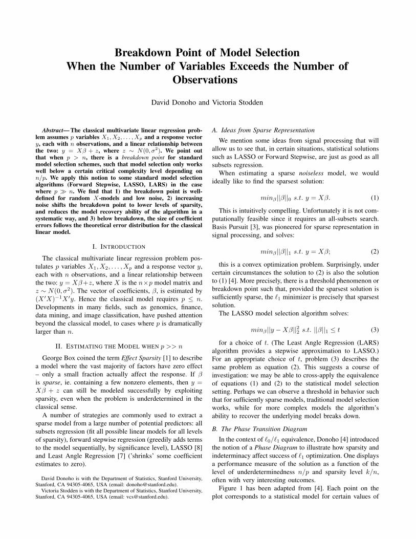
In the context of `0/`1 equivalence, Donoho [4] introducedthe notion of a Phase Diagram to illustrate how sparsity andindeterminacy affect success of `1 optimization. One displaysa performance measure of the solution as a function of thelevel of underdeterminedness n/p and sparsity level k/n,often with very interesting outcomes.

Figure 1 has been adapted from [4]. Each point on theplot corresponds to a statistical model for certain values of

0 0.1 0.2 0.3 0.4 0.5 0.6 0.7 0.8 0.9 10

0.1

0.2

0.3

0.4

0.5

0.6

0.7

0.8

0.9

1

δ = n / p

ρ =

k /

nTheoretical Phase Transition

Combinatorial Search!

Eq (2) solves Eq (1)

Fig. 1. The theoretical threshold at which the l1 approximation to thel0 optimization problem no longer holds. The curve delineates a PhaseTransition from the lower region where the approximation holds, to theupper region, where we are forced to use combinatorial search to recoverthe optimal sparse model. Along the x-axis the level of underdeterminednessdecreases, and along the y-axis the level of sparsity of the underlying modelincreases.

n, p, and k. The abscissa runs from zero to one, and givesvalues for δ = n

p . The ordinate is ρ = kn , measuring the level

of sparsity in the model. Above the plotted phase transitioncurve, the `1 method fails to find the sparsest solution; belowthe curve the solution of (2) is precisely the solution of (1).

Inspired by this approach, we have studied several statis-tical model selection algorithms by the following recipe:

1) Generate underlying model, y = Xβ + z where β issparse i.e. has k < p nonzeros.

2) Run a model selection algorithm, obtaining β̂,3) Evaluate performance: ||β̂−β||2

||β||2 ≤ γ.Averaging the results over numerous realizations, we get a

picture of the performance of model selection as a function ofthe given sparsity and indeterminacy. In this note we presentphase diagrams for LASSO, LARS, Forward Stepwise, andForward Stepwise with False Discovery Rate threshold.

III. MAIN RESULTS

A. Phase Diagrams

For our experiments we specified the underlying model tobe y = Xβ + z where z ∼ N(0, 16), β is zero except for kentries drawn from unif(0, 100), and each Xij ∼ N(0, 1)with columns normalized to unit length.

We display the median of the normalized l2 errors for 30estimated models for each (underdeterminedness, sparsity)combination, p = 200 fixed.

Forward Stepwise enters variables into the model in asequential fashion, according to greatest t-statistic value [9].A

√2 log(p) threshold, or Bonferroni threshold, will admit

terms provided the absolute value of their t-statistic is notless than

√2 log(p), about 3.25 when p = 200. Using

Forward Stepwise with a False Discovery Rate threshold

0.1 0.2 0.3 0.4 0.5 0.6 0.7 0.8 0.9 1

0.1

0.2

0.3

0.4

0.5

0.6

0.7

0.8

0.9

1

δ = n / p

ρ =

k /

n

LASSO Normalized L2 error; Noisy Model z~N(0,16)

0.2

0.3

0.4

0.5

0.6

0.7

0.8

0.9

1

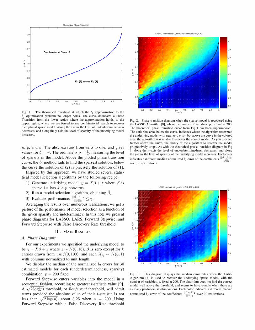
Fig. 2. Phase transition diagram when the sparse model is recovered usingthe LASSO Algorithm [8], where the number of variables, p, is fixed at 200.The theoretical phase transition curve from Fig 1 has been superimposed.The dark blue area, below the curve, indicates where the algorithm recoveredthe underlying model with near zero error, but above the curve in the coloredarea, the algorithm was unable to recover the correct model. As you proceedfurther above the curve, the ability of the algorithm to recover the modelprogressively drops. As with the theoretical phase transition diagram in Fig1, along the x-axis the level of underdeterminedness decreases, and alongthe y-axis the level of sparsity of the underlying model increases. Each colorindicates a different median normalized l2 error of the coefficients ||β̂−β||2

||β||2over 30 realizations.

0.1 0.2 0.3 0.4 0.5 0.6 0.7 0.8 0.9 1

0.1

0.2

0.3

0.4

0.5

0.6

0.7

0.8

0.9

1

δ = n / p

ρ =

k /

n

LARS Normalized l2 error; z~N(0,16); p=200

0.3

0.4

0.5

0.6

0.7

0.8

0.9

1

Fig. 3. This diagram displays the median error rates when the LARSAlgorithm [7] is used to recover the underlying sparse model, with thenumber of variables, p, fixed at 200. The algorithm does not find the correctmodel well above the threshold, and seems to have trouble when there areas many predictors as observations. Each color indicates a different mediannormalized l2 error of the coefficients ||β̂−β||2

||β||2 over 30 realizations.

0.1 0.2 0.3 0.4 0.5 0.6 0.7 0.8 0.9 1

0.1

0.2

0.3

0.4

0.5

0.6

0.7

0.8

0.9

1

δ = n / p

ρ =

k /

n

Normalized L2 Error, sqrt(2log(p)) threshold, z~N(0,42)

0.2

0.4

0.6

0.8

1

1.2

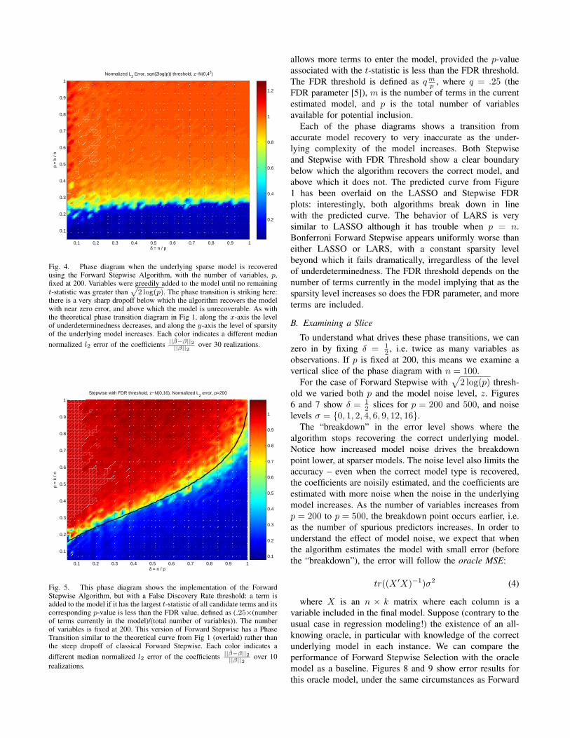
Fig. 4. Phase diagram when the underlying sparse model is recoveredusing the Forward Stepwise Algorithm, with the number of variables, p,fixed at 200. Variables were greedily added to the model until no remainingt-statistic was greater than

p2 log(p). The phase transition is striking here:

there is a very sharp dropoff below which the algorithm recovers the modelwith near zero error, and above which the model is unrecoverable. As withthe theoretical phase transition diagram in Fig 1, along the x-axis the levelof underdeterminedness decreases, and along the y-axis the level of sparsityof the underlying model increases. Each color indicates a different mediannormalized l2 error of the coefficients ||β̂−β||2

||β||2 over 30 realizations.

0.1 0.2 0.3 0.4 0.5 0.6 0.7 0.8 0.9 1

0.1

0.2

0.3

0.4

0.5

0.6

0.7

0.8

0.9

1

δ = n / p

ρ =

k /

n

Stepwise with FDR threshold, z~N(0,16), Normalized L2 error, p=200

0.1

0.2

0.3

0.4

0.5

0.6

0.7

0.8

0.9

1

Fig. 5. This phase diagram shows the implementation of the ForwardStepwise Algorithm, but with a False Discovery Rate threshold: a term isadded to the model if it has the largest t-statistic of all candidate terms and itscorresponding p-value is less than the FDR value, defined as (.25×(numberof terms currently in the model)/(total number of variables)). The numberof variables is fixed at 200. This version of Forward Stepwise has a PhaseTransition similar to the theoretical curve from Fig 1 (overlaid) rather thanthe steep dropoff of classical Forward Stepwise. Each color indicates adifferent median normalized l2 error of the coefficients ||β̂−β||2

||β||2 over 10realizations.

allows more terms to enter the model, provided the p-valueassociated with the t-statistic is less than the FDR threshold.The FDR threshold is defined as q m

p , where q = .25 (theFDR parameter [5]), m is the number of terms in the currentestimated model, and p is the total number of variablesavailable for potential inclusion.

Each of the phase diagrams shows a transition fromaccurate model recovery to very inaccurate as the under-lying complexity of the model increases. Both Stepwiseand Stepwise with FDR Threshold show a clear boundarybelow which the algorithm recovers the correct model, andabove which it does not. The predicted curve from Figure1 has been overlaid on the LASSO and Stepwise FDRplots: interestingly, both algorithms break down in linewith the predicted curve. The behavior of LARS is verysimilar to LASSO although it has trouble when p = n.Bonferroni Forward Stepwise appears uniformly worse thaneither LASSO or LARS, with a constant sparsity levelbeyond which it fails dramatically, irregardless of the levelof underdeterminedness. The FDR threshold depends on thenumber of terms currently in the model implying that as thesparsity level increases so does the FDR parameter, and moreterms are included.

B. Examining a Slice

To understand what drives these phase transitions, we canzero in by fixing δ = 1

2 , i.e. twice as many variables asobservations. If p is fixed at 200, this means we examine avertical slice of the phase diagram with n = 100.

For the case of Forward Stepwise with√

2 log(p) thresh-old we varied both p and the model noise level, z. Figures6 and 7 show δ = 1

2 slices for p = 200 and 500, and noiselevels σ = {0, 1, 2, 4, 6, 9, 12, 16}.

The “breakdown” in the error level shows where thealgorithm stops recovering the correct underlying model.Notice how increased model noise drives the breakdownpoint lower, at sparser models. The noise level also limits theaccuracy – even when the correct model type is recovered,the coefficients are noisily estimated, and the coefficients areestimated with more noise when the noise in the underlyingmodel increases. As the number of variables increases fromp = 200 to p = 500, the breakdown point occurs earlier, i.e.as the number of spurious predictors increases. In order tounderstand the effect of model noise, we expect that whenthe algorithm estimates the model with small error (beforethe “breakdown”), the error will follow the oracle MSE:

tr((X ′X)−1)σ2 (4)

where X is an n × k matrix where each column is avariable included in the final model. Suppose (contrary to theusual case in regression modeling!) the existence of an all-knowing oracle, in particular with knowledge of the correctunderlying model in each instance. We can compare theperformance of Forward Stepwise Selection with the oraclemodel as a baseline. Figures 8 and 9 show error results forthis oracle model, under the same circumstances as Forward

Stepwise: δ = 12 slices for p = 200 and 500, and noise levels

σ = {0, 1, 2, 4, 6, 9, 12, 16}. For both p = 200 and p = 500the median oracle MSE increases proportionally to the modelnoise level.

0 0.1 0.2 0.3 0.4 0.5 0.6 0.7 0.8 0.9 10

0.2

0.4

0.6

0.8

1

1.2

1.4

ρ = k / n

Normalized L2 Error for δ = .5, p=200. Stepwise with sqrt(2logp) threshold

z~N(0,162)

z~N(0,122)

z~N(0,92)

z~N(0,62)

z~N(0,42)

z~N(0,22)

z~N(0,12)no noise

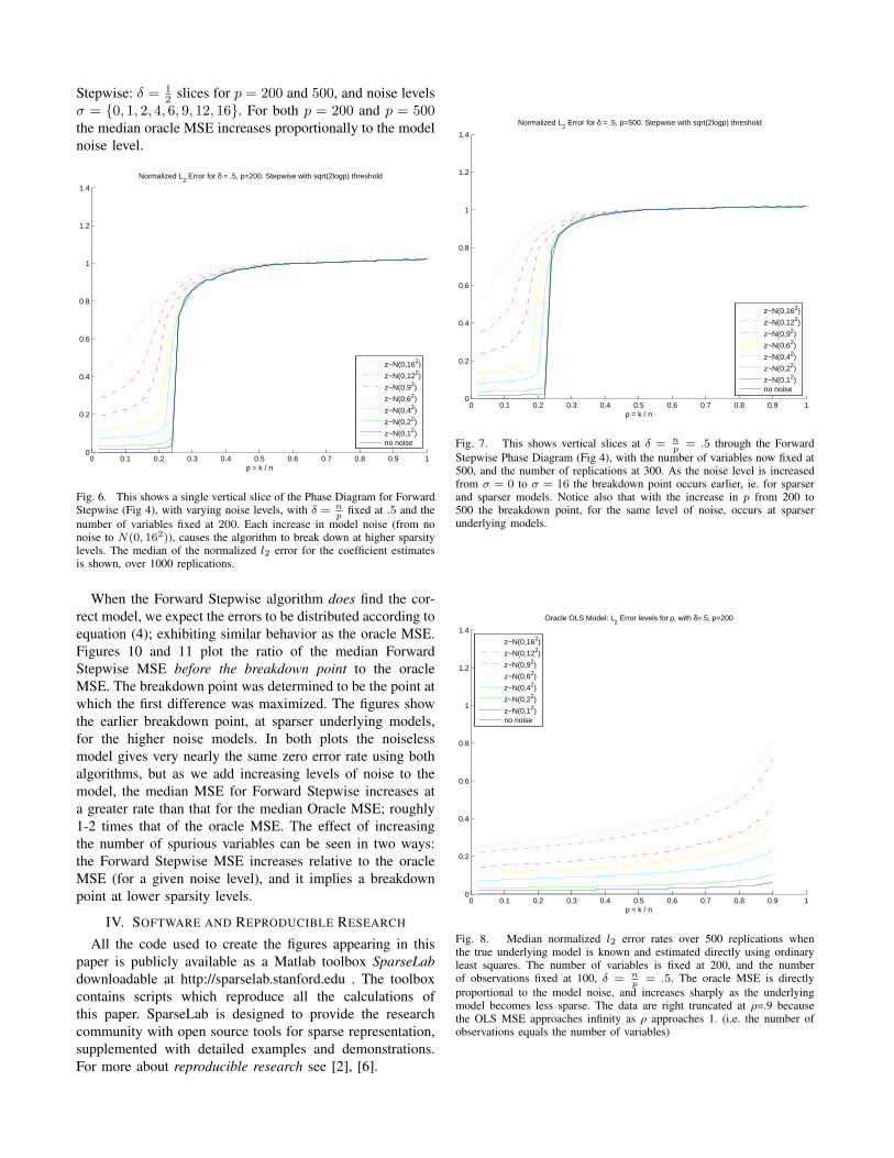
Fig. 6. This shows a single vertical slice of the Phase Diagram for ForwardStepwise (Fig 4), with varying noise levels, with δ = n

pfixed at .5 and the

number of variables fixed at 200. Each increase in model noise (from nonoise to N(0, 162)), causes the algorithm to break down at higher sparsitylevels. The median of the normalized l2 error for the coefficient estimatesis shown, over 1000 replications.

When the Forward Stepwise algorithm does find the cor-rect model, we expect the errors to be distributed according toequation (4); exhibiting similar behavior as the oracle MSE.Figures 10 and 11 plot the ratio of the median ForwardStepwise MSE before the breakdown point to the oracleMSE. The breakdown point was determined to be the point atwhich the first difference was maximized. The figures showthe earlier breakdown point, at sparser underlying models,for the higher noise models. In both plots the noiselessmodel gives very nearly the same zero error rate using bothalgorithms, but as we add increasing levels of noise to themodel, the median MSE for Forward Stepwise increases ata greater rate than that for the median Oracle MSE; roughly1-2 times that of the oracle MSE. The effect of increasingthe number of spurious variables can be seen in two ways:the Forward Stepwise MSE increases relative to the oracleMSE (for a given noise level), and it implies a breakdownpoint at lower sparsity levels.

IV. SOFTWARE AND REPRODUCIBLE RESEARCH

All the code used to create the figures appearing in thispaper is publicly available as a Matlab toolbox SparseLabdownloadable at http://sparselab.stanford.edu . The toolboxcontains scripts which reproduce all the calculations ofthis paper. SparseLab is designed to provide the researchcommunity with open source tools for sparse representation,supplemented with detailed examples and demonstrations.For more about reproducible research see [2], [6].

0 0.1 0.2 0.3 0.4 0.5 0.6 0.7 0.8 0.9 10

0.2

0.4

0.6

0.8

1

1.2

1.4

ρ = k / n

Normalized L2 Error for δ = .5, p=500. Stepwise with sqrt(2logp) threshold

z~N(0,162)

z~N(0,122)

z~N(0,92)

z~N(0,62)

z~N(0,42)

z~N(0,22)

z~N(0,12)no noise

Fig. 7. This shows vertical slices at δ = np

= .5 through the ForwardStepwise Phase Diagram (Fig 4), with the number of variables now fixed at500, and the number of replications at 300. As the noise level is increasedfrom σ = 0 to σ = 16 the breakdown point occurs earlier, ie. for sparserand sparser models. Notice also that with the increase in p from 200 to500 the breakdown point, for the same level of noise, occurs at sparserunderlying models.

0 0.1 0.2 0.3 0.4 0.5 0.6 0.7 0.8 0.9 10

0.2

0.4

0.6

0.8

1

1.2

1.4

ρ = k / n

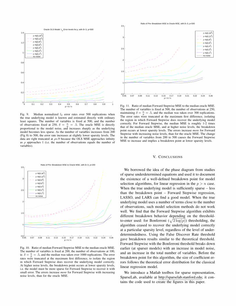
Oracle OLS Model: L2 Error levels for ρ, with δ=.5, p=200

z~N(0,162)

z~N(0,122)

z~N(0,92)

z~N(0,62)

z~N(0,42)

z~N(0,22)

z~N(0,12)no noise

Fig. 8. Median normalized l2 error rates over 500 replications whenthe true underlying model is known and estimated directly using ordinaryleast squares. The number of variables is fixed at 200, and the numberof observations fixed at 100, δ = n

p= .5. The oracle MSE is directly

proportional to the model noise, and increases sharply as the underlyingmodel becomes less sparse. The data are right truncated at ρ=.9 becausethe OLS MSE approaches infinity as ρ approaches 1. (i.e. the number ofobservations equals the number of variables)

0 0.1 0.2 0.3 0.4 0.5 0.6 0.7 0.8 0.9 10

0.2

0.4

0.6

0.8

1

1.2

1.4

ρ = k / n

Oracle OLS Model: L2 Error levels for ρ, with δ=.5, p=500

z~N(0,162)

z~N(0,122)

z~N(0,92)

z~N(0,62)

z~N(0,42)

z~N(0,22)

z~N(0,12)no noise

Fig. 9. Median normalized l2 error rates over 500 replications whenthe true underlying model is known and estimated directly with ordinaryleast squares. The number of variables is fixed at 500, and the numberof observations fixed at 250, δ = n

p= .5. The oracle MSE is directly

proportional to the model noise, and increases sharply as the underlyingmodel becomes less sparse. As the number of variables increases from 200(Fig 8) to 500, the error rate increases at slightly lower sparsity levels. Thedata are right truncated at ρ=.9 because the OLS MSE approaches infinityas ρ approaches 1 (i.e. the number of observations equals the number ofvariables).

0.05 0.07 0.09 0.11 0.13 0.15 0.17 0.19 0.21 0.22 0.24 0.260.5

1

1.5

2

2.5

3

3.5

ρ = k / n

Ratio of Pre−Breakdown MSE to Oracle MSE, with δ=.5, p=200

z~N(0,162)

z~N(0,122)

z~N(0,92)

z~N(0,62)

z~N(0,42)

z~N(0,22)

z~N(0,12)no noise

Fig. 10. Ratio of median Forward Stepwise MSE to the median oracle MSE.The number of variables is fixed at 200, the number of observations at 100,ie. δ = n

p= .5, and the median was taken over 1000 replications. The error

rates were truncated at the maximum first difference, to isolate the regionin which Forward Stepwise does recover the underlying model correctly.At higher noise levels, the breakdown point occurs at lower sparsity levels,i.e. the model must be more sparse for Forward Stepwise to recover it withsmall error. The errors increase more for Forward Stepwise with increasingnoise levels, than for the oracle MSE.

0.05 0.07 0.09 0.11 0.13 0.15 0.17 0.19 0.21 0.22 0.24 0.260.5

1

1.5

2

2.5

3

3.5

ρ = k / n

Ratio of Pre−Breakdown MSE to Oracle MSE, with δ=.5, p=500

z~N(0,162)

z~N(0,122)

z~N(0,92)

z~N(0,62)

z~N(0,42)

z~N(0,22)

z~N(0,12)no noise

Fig. 11. Ratio of median Forward Stepwise MSE to the median oracle MSE.The number of variables is fixed at 500, the number of observations at 250,maintaining δ = n

p= .5, and the median was taken over 300 replications.

The error rates were truncated at the maximum first difference, isolatingthe region in which Forward Stepwise does recover the underlying modelcorrectly. For Forward Stepwise, the median MSE is roughly 1-2 timesthat of the median oracle MSE, and at higher noise levels, the breakdownpoint occurs at lower sparsity levels. The errors increase more for ForwardStepwise with increasing noise levels, than for the oracle MSE. The changein the number of variables from 200 to 500 causes the Forward StepwiseMSE to increase and implies a breakdown point at lower sparsity levels.

V. CONCLUSIONS

We borrowed the idea of the phase diagram from studiesof sparse underdetermined equations and used it to documentthe existence of a well-defined breakdown point for modelselection algorithms, for linear regression in the p > n case.When the true underlying model is sufficiently sparse – lessthan the breakdown point – Forward Stepwise regression,LASSO, and LARS can find a good model. When the trueunderlying model uses a number of terms close to the numberof observations, such model selection methods do not workwell. We find that the Forward Stepwise algorithm exhibitsdifferent breakdown behavior depending on the threshold-to-enter used: for Bonferroni (

√2 log(p)) thresholding, the

algorithm ceased to recover the underlying model correctlyat a particular sparsity level, regardless of the level of under-determindedness. Using the False Discover Rate thresholdgave breakdown results similar to the theoretical threshold.Forward Stepwise with the Bonferroni threshold breaks downearlier (at sparser models) with an increase in model noise,and an increase in the total number of variables. Before thebreakdown point for this algorithm, the size of coefficient er-rors follows the theoretical error distribution for the classicallinear regression model.

We introduce a Matlab toolbox for sparse representation,SparseLab, available at http://sparselab.stanford.edu; it con-tains the code used to create the figures in this paper.

ACKNOWLEDGMENT

The authors would like to thank Iddo Drori and YaakovTsaig for useful discussions. This work was supported inpart by the National Science Foundation under grant DMS-05-05303.

REFERENCES

[1] G. Box, D. Meyer, “An Analysis for Unreplicated Fractional Factorials”Technometrics Vol. 28, No. 1, pp 11-18, 1986.

[2] J. Buckheit, D. Donoho, “WaveLab and Reproducible Research,” in A.Antoniadis, Editor, Wavelets and Statistics, Springer, 1995.

[3] S. Chen, D. Donoho, M. Saunders, “Atomic Decomposition by BasisPursuit,” SIAM Review, Vol. 43, Issue 1, pp. 129-159, 2001.

[4] D. Donoho, “High-Dimensional Centrosymmetric Polytopes withNeighborliness Proportional to Dimension” Discrete and ComputationalGeometry, online first edition, December 22, 2005.

[5] D. Donoho, J. Jin, “Asymptotic Minimaxity of FDR Thresholding forSparse Mixtures of Exponentials” Ann. Stat., to appear.

[6] D. Donoho, X. Huo, “Beamlab and Reproducible Research,” Interna-tional Journal of Wavelets, Multiresolution and Information Processing,vol. 2, No. 4, pp. 391-414, 2004.

[7] B. Efron, T. Hastie, I. Johnstone, R. Tibshirani, “Least Angle Regres-sion,” Ann. Statist., vol. 32, No. 2, pp. 407-499, 2004.

[8] R. Tibshirani, “Regression Shrinkage and Selection via the Lasso,” J.Royal. Statist. Soc B., vol. 58, No. 1, pp. 267–288, 1996.

[9] S. Weisberg, Applied Linear Regression 2nd ed., John Wiley & Sons,1985.