Bond Graph Model of a Vertical U-Tube Steam Condenser Coupled with a

Heat Exchanger

K. Medjaher1+ A.K. Samantaray2 B. Ould Bouamama3

1LAB, CNRS UMR 6596, ENSMM de Besançon, 26 Chemin de l’Epitaphe, 25030 Besançon, France 2Department of Mechanical Engineering, Indian Institute of Technology, 721302 Kharagpur, India

3LAGIS, CNRS UMR 8146, Université de Lille-1, 59655 Villeneuve d’Ascq Cedex, France

Abstract

A simulation model for a vertical U-tube steam condenser in which the condensate is stored at the bottom well is developed in this paper. The U-tubes carrying the coolant are partially submerged in the stored condensate and thus the bottom well acts as a heat exchanger. The storage of hydraulic and thermal energies is represented using a coupled pseudo-bond graph model. Advection effects are modelled by considering reticulated segments of the tubes carrying coolant, over which condensation takes place. The developed model is of intermediate complexity and it is intended for use in observer based real time process supervision, which works by comparing the process behaviour to the reference model outputs. The simulation results obtained from the bond graph model are validated with experimental data from a laboratory set-up.

Keywords: Vertical steam condenser; Heat exchanger; Bond graph

1. Introduction

Modern process engineering plants are designed to reuse the material and energy for improving the process efficiency and also to reduce production costs. The process dynamics of such systems is usually complex and consequently designing them for optimal utilisation of resources requires a well-developed simulation model. However, each component’s model must not be too complex because the component’s model is not only used for simulation of the single process component’s behaviour, but also used to predict the overall steady state and dynamic response of the process. Furthermore, process models are being increasingly used for online monitoring, diagnosis of process faults, and fault tolerant control; and this requires real time computations of the model output for comparison with the actual process behaviour. Therefore, one needs faster numerical computation using a simplified, but accurate process model.

In this paper, model of a vertical U-tube steam condenser coupled with a heat exchanger is developed and the model complexity is limited to the intermediate level. Steam condensers are integral part of any nuclear and thermal power plant utilising steam turbines, distillation industries using water as a solvent, etc. System-level modeling of steam condensers has to consider both mass and energy balances in two control volumes, namely steam and condensate, and energy balance in further two control volumes, namely tubes and the coolant flowing through them. That is why bond graph modelling as a multi-energy

+ Corresponding author Tel: +33 03 81 40 27 95 Email: Kamal.medjaher@ens2m.fr

Manuscript submitted to Simulation Modelling Practice and Theory.

domain approach is a suitable tool for representing such systems [1-5]. Furthermore, the conservative nature of junction structure in a bond graph model ensures that the material and energy balances are correctly represented in each step.

The literature on bond graph modeling of heat exchangers is pervasive [6-10]. They are based on pseudo-bond graph representations of thermo-fluid transport and heat exchange developed in [11-14]. Thoma [2, 10] has even introduced the term ‘HEXA’, as a generic nomenclature, for the bond graph sub-model of a heat exchanger.

On the other hand, very few works on bond graph modeling of condensers are reported in literature. Some of the works on bond graph modeling of condensation phenomena assume bulk condensation (similar to cloud formation and its saturation) and base the analysis on the relative humidity [15-16] in the control volume. Other bond graph formulations for storage and transport of two-phase mixtures (water and steam mixture, here) may be consulted in [17-18]. Bond graph representations of film condensation on vertical tubes were developed in [10, 19-20]. However, the film condensation models developed therein are inaccurate because they assume the entire segments of the tube to be at uniform temperature. In this paper, we consider the temperature variation in the tube by considering several small and finite segments. This approach for bond graph modeling of distributed-parameter multiphase thermodynamic systems has been developed in [17] by using convection bonds. Further note that a pseudo-bond graph model of a U-tube steam generator (boiler) has been developed in [21] by using one-dimensional finite-element modeling concept, which is similar to the one followed in this paper.

2. Modelling

Steam condensation involves both convection and conduction [22-23]. In process engineering systems, it is simpler to use enthalpy flow instead of entropy flow to model heat convection using pseudo-bond graph representation [10-14]. In this paper, pressure and temperature are considered as the generalised effort variables, and mass flow rate and enthalpy flow rate are taken as the generalised flow variables. The convection heat transfer due to mass flow is represented using inter-domain couplings presented in [20]. Note that a simpler model for this type of condenser has been developed in [20] for fault detection.

2.1. Description of the condenser

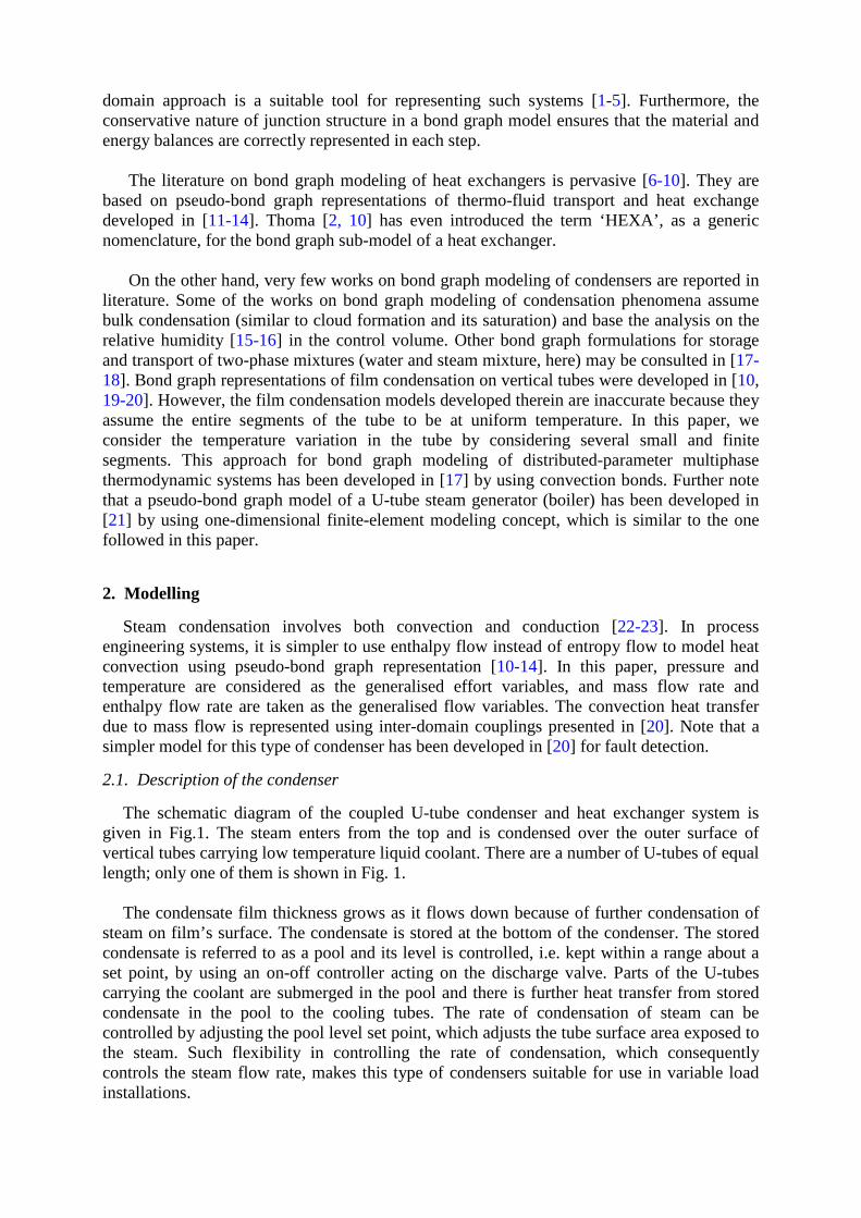
The schematic diagram of the coupled U-tube condenser and heat exchanger system is given in Fig.1. The steam enters from the top and is condensed over the outer surface of vertical tubes carrying low temperature liquid coolant. There are a number of U-tubes of equal length; only one of them is shown in Fig. 1.

The condensate film thickness grows as it flows down because of further condensation of

steam on film’s surface. The condensate is stored at the bottom of the condenser. The stored condensate is referred to as a pool and its level is controlled, i.e. kept within a range about a set point, by using an on-off controller acting on the discharge valve. Parts of the U-tubes carrying the coolant are submerged in the pool and there is further heat transfer from stored condensate in the pool to the cooling tubes. The rate of condensation of steam can be controlled by adjusting the pool level set point, which adjusts the tube surface area exposed to the steam. Such flexibility in controlling the rate of condensation, which consequently controls the steam flow rate, makes this type of condensers suitable for use in variable load installations.

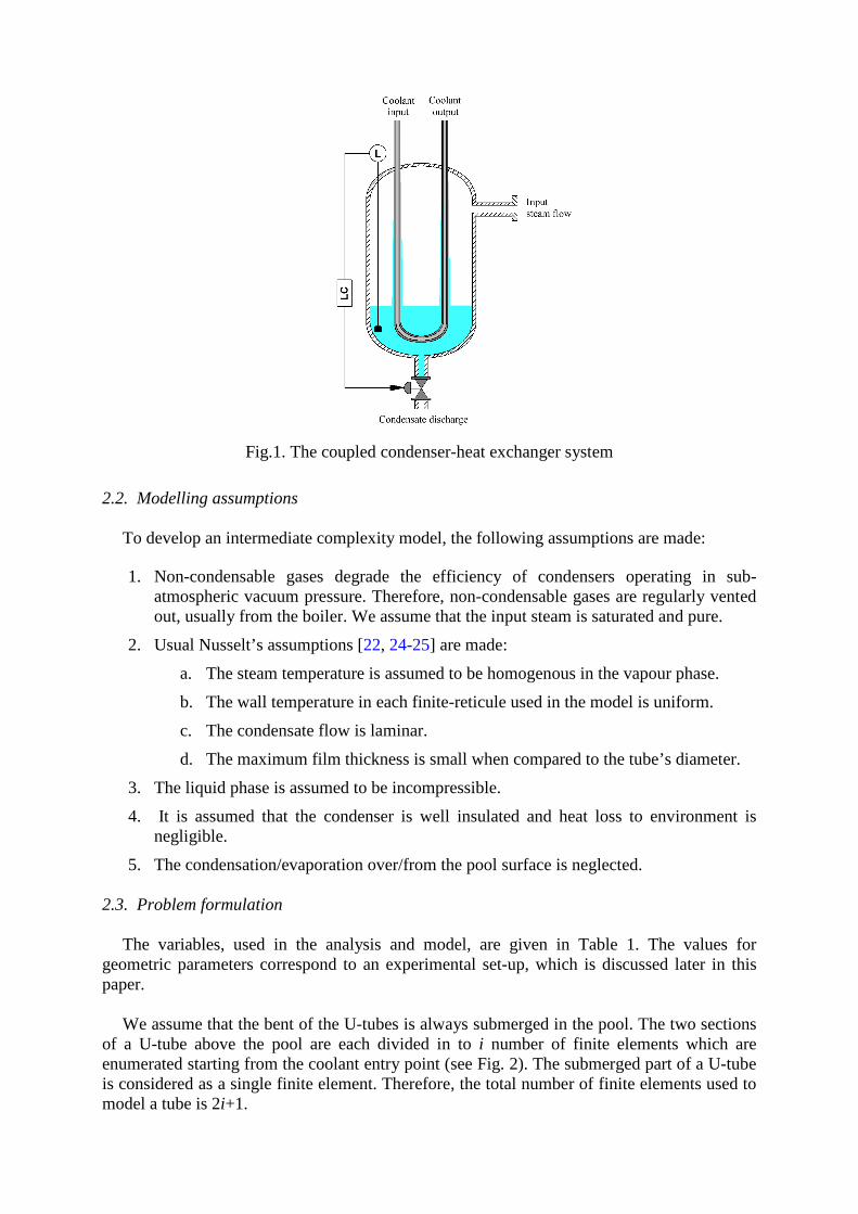
Fig.1. The coupled condenser-heat exchanger system

2.2. Modelling assumptions

To develop an intermediate complexity model, the following assumptions are made:

1. Non-condensable gases degrade the efficiency of condensers operating in sub-atmospheric vacuum pressure. Therefore, non-condensable gases are regularly vented out, usually from the boiler. We assume that the input steam is saturated and pure.

2. Usual Nusselt’s assumptions [22, 24-25] are made:

a. The steam temperature is assumed to be homogenous in the vapour phase.

b. The wall temperature in each finite-reticule used in the model is uniform.

c. The condensate flow is laminar.

d. The maximum film thickness is small when compared to the tube’s diameter.

3. The liquid phase is assumed to be incompressible.

4. It is assumed that the condenser is well insulated and heat loss to environment is negligible.

5. The condensation/evaporation over/from the pool surface is neglected.

2.3. Problem formulation

The variables, used in the analysis and model, are given in Table 1. The values for geometric parameters correspond to an experimental set-up, which is discussed later in this paper.

We assume that the bent of the U-tubes is always submerged in the pool. The two sections of a U-tube above the pool are each divided in to i number of finite elements which are enumerated starting from the coolant entry point (see Fig. 2). The submerged part of a U-tube is considered as a single finite element. Therefore, the total number of finite elements used to model a tube is 2i+1.

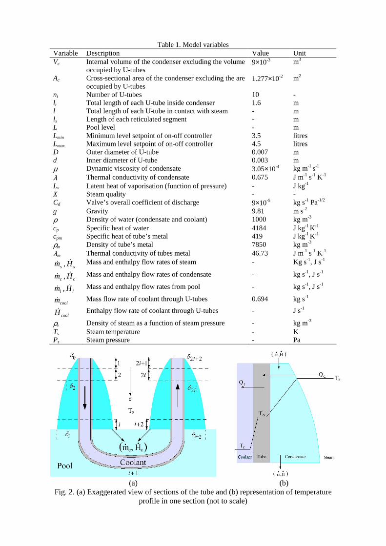
Table 1. Model variables Variable Description Value Unit Vc Internal volume of the condenser excluding the volume

occupied by U-tubes 9×10-3

m3

Ac Cross-sectional area of the condenser excluding the are occupied by U-tubes

1.277×10-2 m2

nt Number of U-tubes 10 - l t Total length of each U-tube inside condenser 1.6 m l Total length of each U-tube in contact with steam - m ls Length of each reticulated segment - m L Pool level - m Lmin Minimum level setpoint of on-off controller 3.5 litres Lmax Maximum level setpoint of on-off controller 4.5 litres D Outer diameter of U-tube 0.007 m d Inner diameter of U-tube 0.003 m µ Dynamic viscosity of condensate 3.05×10-4 kg m-1 s-1 λ Thermal conductivity of condensate 0.675 J m-1 s-1 K-1 Lv Latent heat of vaporisation (function of pressure) - J kg-1 X Steam quality - - Cd Valve’s overall coefficient of discharge 9×10-5 kg s-1 Pa-1/2 g Gravity 9.81 m s-2 ρ Density of water (condensate and coolant) 1000 kg m-3 cp Specific heat of water 4184 J kg-1 K-1 cpm Specific heat of tube’s metal 419 J kg-1 K-1 ρm Density of tube’s metal 7850 kg m-3 λm Thermal conductivity of tubes metal 46.73 J m-1 s-1 K-1

smɺ , sHɺ Mass and enthalpy flow rates of steam - Kg s-1, J s-1

cmɺ , cHɺ Mass and enthalpy flow rates of condensate - kg s-1, J s-1

lmɺ , lHɺ Mass and enthalpy flow rates from pool - kg s-1, J s-1

coolmɺ Mass flow rate of coolant through U-tubes 0.694 kg s-1

coolHɺ Enthalpy flow rate of coolant through U-tubes - J s-1

ρv Density of steam as a function of steam pressure - kg m-3 Ts Steam temperature - K Ps Steam pressure - Pa

(a) (b)

Fig. 2. (a) Exaggerated view of sections of the tube and (b) representation of temperature profile in one section (not to scale)

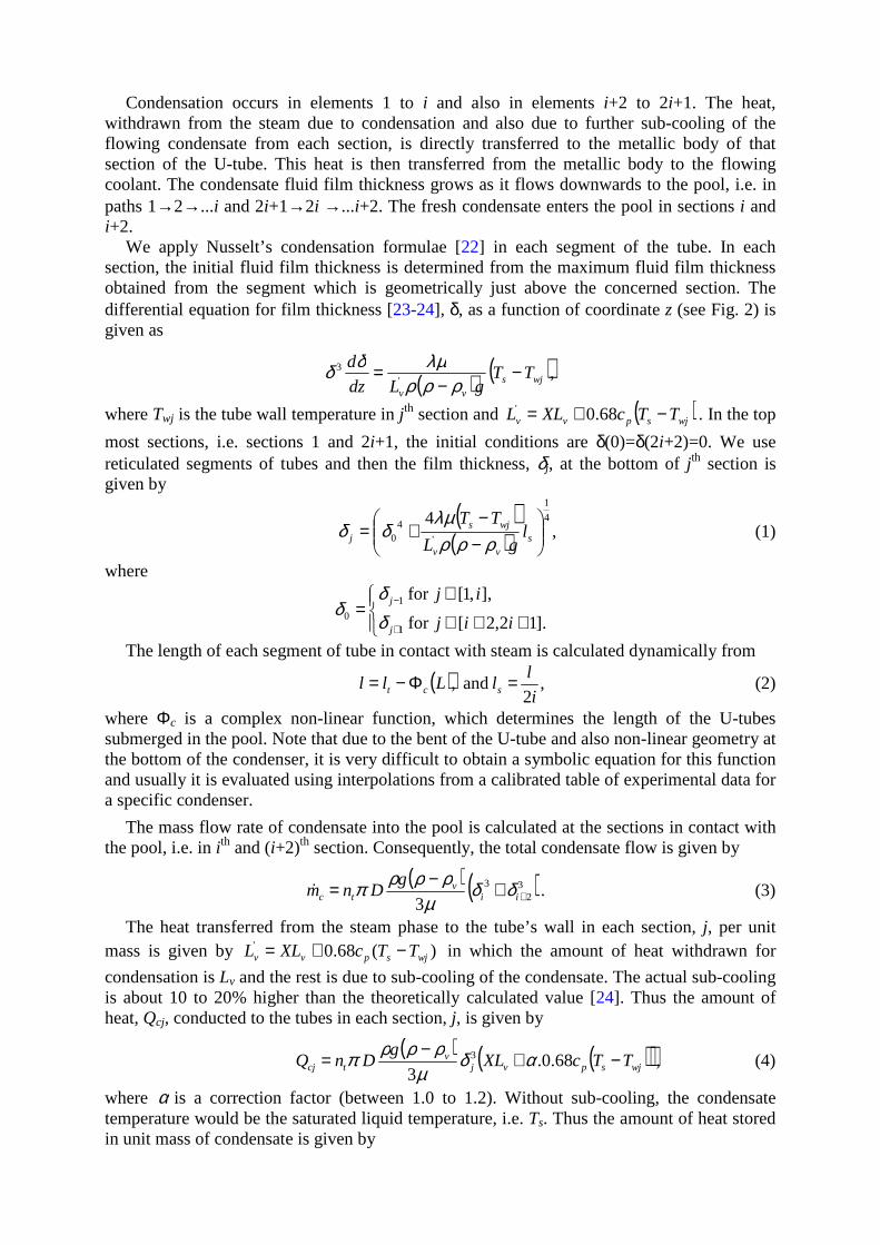
Condensation occurs in elements 1 to i and also in elements i+2 to 2i+1. The heat, withdrawn from the steam due to condensation and also due to further sub-cooling of the flowing condensate from each section, is directly transferred to the metallic body of that section of the U-tube. This heat is then transferred from the metallic body to the flowing coolant. The condensate fluid film thickness grows as it flows downwards to the pool, i.e. in paths 1→2→...i and 2i+1→2i →...i+2. The fresh condensate enters the pool in sections i and i+2.

We apply Nusselt’s condensation formulae [22] in each segment of the tube. In each section, the initial fluid film thickness is determined from the maximum fluid film thickness obtained from the segment which is geometrically just above the concerned section. The differential equation for film thickness [23-24], δ, as a function of coordinate z (see Fig. 2) is given as

( ) ( ),'

3wjs

vv

TTgLdz

d −−

=ρρρ

λµδδ

where Twj is the tube wall temperature in j th section and ( )wjspvv TTcXLL −+= 68.0' . In the top

most sections, i.e. sections 1 and 2i+1, the initial conditions are δ(0)=δ(2i+2)=0. We use reticulated segments of tubes and then the film thickness, δj, at the bottom of j th section is given by

( )( ) ,

4 4

1

'

40

−−

+= svv

wjsj l

gL

TT

ρρρλµ

δδ (1)

where

++∈

∈=

+

−

].12,2[for

],,1[for

1

1

0 iij

ij

j

j

δδ

δ

The length of each segment of tube in contact with steam is calculated dynamically from

( ) ,2

and ,i

llLll sct =Φ−= (2)

where Φc is a complex non-linear function, which determines the length of the U-tubes submerged in the pool. Note that due to the bent of the U-tube and also non-linear geometry at the bottom of the condenser, it is very difficult to obtain a symbolic equation for this function and usually it is evaluated using interpolations from a calibrated table of experimental data for a specific condenser.

The mass flow rate of condensate into the pool is calculated at the sections in contact with the pool, i.e. in i th and (i+2)th section. Consequently, the total condensate flow is given by

( ) ( )32

3

3 ++−= ii

vtc

gDnm δδ

µρρρπɺ . (3)

The heat transferred from the steam phase to the tube’s wall in each section, j, per unit mass is given by )(68.0'

wjspvv TTcXLL −+= in which the amount of heat withdrawn for

condensation is Lv and the rest is due to sub-cooling of the condensate. The actual sub-cooling is about 10 to 20% higher than the theoretically calculated value [24]. Thus the amount of heat, Qcj, conducted to the tubes in each section, j, is given by

( ) ( )( )wjspvjv

tcj TTcXLg

DnQ −+−= 68.0.3

3 αδµ

ρρρπ , (4)

where α is a correction factor (between 1.0 to 1.2). Without sub-cooling, the condensate temperature would be the saturated liquid temperature, i.e. Ts. Thus the amount of heat stored in unit mass of condensate is given by

)(68.0 wjspsp TTcTc −− α . (5)

Then the total enthalpy flow into the pool from sections i and i+2 is given by ( ) ( ) ( )( )( ),)(68.0)(68.03 )2(

32

3++ −−+−−−= iwssiwissi

vptc TTTTTT

gDcnH αδαδ

µρρρπɺ (6)

where Twi and Tw(i+2) are respectively the tube wall temperatures in sections i and i+2.

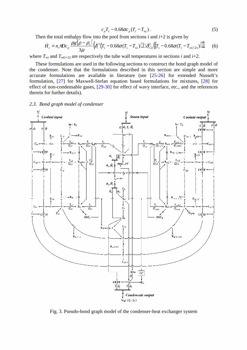
These formulations are used in the following sections to construct the bond graph model of the condenser. Note that the formulations described in this section are simple and more accurate formulations are available in literature (see [25-26] for extended Nusselt’s formulation, [27] for Maxwell-Stefan equation based formulations for mixtures, [28] for effect of non-condensable gases, [29-30] for effect of wavy interface, etc., and the references therein for further details). 2.3. Bond graph model of condenser

Fig. 3. Pseudo-bond graph model of the condenser-heat exchanger system

The pseudo-bond graph model of the vertical condenser-heat exchanger system is given in Fig.3. The bonds and signals with a circle over them are vectors [10]. Thick perpendicular lines are used to decompose vector bonds and signals to their scalar forms and vice versa.

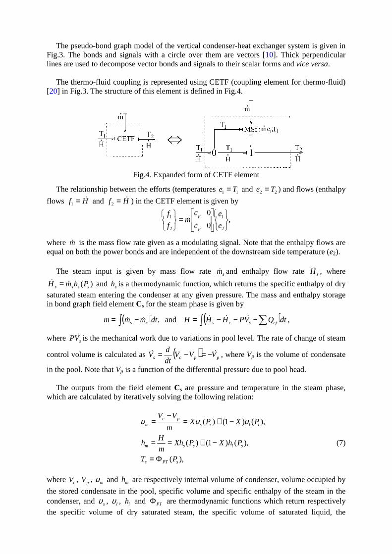
The thermo-fluid coupling is represented using CETF (coupling element for thermo-fluid) [20] in Fig.3. The structure of this element is defined in Fig.4.

Fig.4. Expanded form of CETF element

The relationship between the efforts (temperatures 11 Te = and 22 Te = ) and flows (enthalpy

flows Hf ɺ=1 and Hf ɺ=2 ) in the CETF element is given by

,0

0

2

1

2

1

=

e

e

c

cm

f

f

p

pɺ

where mɺ is the mass flow rate given as a modulating signal. Note that the enthalpy flows are equal on both the power bonds and are independent of the downstream side temperature (e2).

The steam input is given by mass flow rate smɺ and enthalpy flow rate sHɺ , where

)( ssss PhmH ɺɺ = and sh is a thermodynamic function, which returns the specific enthalpy of dry

saturated steam entering the condenser at any given pressure. The mass and enthalpy storage in bond graph field element Cs for the steam phase is given by

( ) ( )∫ ∑∫ −−−=−= dtQVPHH Hdtmmm cjscscsɺɺɺɺɺ and , ,

where sVP ɺ is the mechanical work due to variations in pool level. The rate of change of steam

control volume is calculated as ( ) ppcs VVVdt

dV ɺɺ −=−= , where Vp is the volume of condensate

in the pool. Note that Vp is a function of the differential pressure due to pool head.

The outputs from the field element Cs are pressure and temperature in the steam phase, which are calculated by iteratively solving the following relation:

),(

),()1()(

),()1()(

sPTs

slssm

llsspc

m

PT

PhXPXhm

Hh

PXPXm

VV

Φ=

−+==

−+=−

= υυυ

(7)

where cV , pV , mυ and mh are respectively internal volume of condenser, volume occupied by

the stored condensate in the pool, specific volume and specific enthalpy of the steam in the condenser, and sυ , lυ , lh and PTΦ are thermodynamic functions which return respectively

the specific volume of dry saturated steam, the specific volume of saturated liquid, the

specific enthalpy of saturated liquid, and the temperature of saturated steam, at any given pressure. From Eq.(7), the steam quality (X) and steam pressure (Ps) are solved iteratively using bisection method and the result is then used to calculate steam temperature (Ts). An alternative way of modelling storage of mixtures, which does not involve an iterative solution and uses different set of state variables, is given in [18].

The condensate storage in the pool is represented by the bond graph element Ch for hydraulic energy and element Ct for thermal energy. In this case, it is possible to separate the hydraulic and thermal energy storage by assuming that the condensate is incompressible and is in an under-saturated state.

Element Ch produces the differential pressure head (Pl) or pool level (L), defined by the following relations:

( )( ),dtmmP lcpl ∫ −Φ= ɺɺ (8)

where lmɺ is the rate of condensate discharge and PΦ is a function, which depends on the

geometry of the condenser (it is usually obtained using experimental calibration). In the simplest case, assuming a cylindrical condenser, Eq.(8) may be rewritten as

( )( )dtmmC

P lch

l ∫ −= ɺɺ1

, where .g

AC c

h =

The storage of thermal energy in the pool liquid is modelled using modulated bond graph

element Ct. Its constitutive relation is given by

( )( )

( )( )lpp

lc

lcp

lc

l Pc

dtHH

dtmmc

dtHHT 1

−Φ

−=

−

−= ∫

∫∫ ɺɺ

ɺɺ

ɺɺ

, (9)

where lHɺ is the rate of enthalpy flow with condensate discharge and Tl is the pool

temperature. Assuming a cylindrical condenser, Eq. (9) can be rewritten as

( )dtHHC

T lct

l 1∫ −= ɺɺ , where .l

cpt P

g

AcC

= (10)

The condensate discharge, represented by bond graph element RV and the enthalpy flow associated CETF element are given as

( ),

,,

lpll

dsldvl

TcmH

PPPuCm

ɺɺ

ɺ

=

−+Φ= (11)

where u is the controller signal, ),( uCdvΦ is a function that determines the overall discharge

coefficient of the valve, which depends on the constructional features of the valve and its characteristics (linear, quadratic, quick opening, equal percentage, etc.). Note that at junction 1b, the upstream pressure is sum of differential pool pressure and the steam pressure. The pool level controller, represented by block element LC, is defined as follows:

≤

≥=

,for ,0

,for ,1

min

max

LL

LLu

p

p (12)

where .g

PL l

p ρ=

The condensation phenomena, given by Eq. (1), Eqs. (3-4) and Eq.(6), are represented by elements Rnj for the j th section. The inputs are the steam temperature (Ts), pool level (calculated from Pl and used to determine ls from Eq. (2)) and the wall temperature Twj. The outputs are the heat flowing from steam to condensate (Qci), the mass and enthalpy flow rates of condensate ( cc Hm ɺɺ and ), and the maximum fluid film thickness δj, which is used in

Nusselt’s relation of section that is vertically below the considered section.

The heat capacity of the tube in j th section is represented by element Ctj, whose value is determined as follows:

( )22

4dDlcnC jmpmttj −= πρ , (13)

where l j is the length of j th section. For j =1..i and j =(i+1)..(2i), l j = l s. For the section submerged in the pool, i.e. j = i, sj illl 2−= . Likewise, the heat capacity of the coolant in j th

section is represented by element Ccj and its value is determined from

.4

2dlcnC jptcj

πρ= (14)

Element Rtj_k represents longitudinal heat transfer resistance between j th and kth (consecutive) sections of the metal tube. Transverse heat transfer resistance between the metal tube and the coolant in j th section (depends on the coolant flow rate) is represented by element Rctj. Convection heat transfer coefficient hml is obtained experimentally. Heat transfer resistance between liquid and the metal tube submerged in the pool is represented by element Rtl. Heat transfer resistance between topmost segments of the tube and the un-modelled external segments exposed to the environment is modelled by element Rto. The values for these elements are obtained as follows:

( )( )22_

2

dDn

llR

mt

kjktj −

+=

πλ,

jmtmlstctj ln

d

dD

hdlnR

πλπ 22

ln1

+

+= ,

( )smttl illn

dD

D

R22

2ln

−

+=πλ

,

( ).2

22 dDn

lR

mt

sto −

=πλ

(15)

Junctions 0Qi and 0Qo are used to sum the total heat transferred to the tubes from steam in

the coolant inlet side and the coolant outlet side of the tube, respectively, i.e. ∑=

==

ij

jcjcin QQ

1

,

and . ,12

2cocinc

ij

ijcjco QQQQQ +== ∑

+=

+=

Modulated sources MSfi and MSfo model the condensate

mass and enthalpy flow rates (in vector form), respectively from i th and (i+2)th sections to the pool. Their relations are given by Eq. (3) and Eq.(6). Junction 0c is used to sum MSfi and MSfo. In steady state, the condensate flow rate is assumed to be equal to the rate of

condensation. Thus, these mass and enthalpy flow rates represent the transfer of mass and energy from steam phase to the pool.

Note that the liquid phase is considered incompressible and all those elements whose

relations involve the pool level L (alternatively, volume Vp and pressure Pl) are in fact modulated (e.g. Ctj, Rctj, Ccj, for j=1...2i+1). These modulations are not shown in the model to maintain clarity of presentation.

The rest of the elements in the bond graph model given in Fig.3 are simple and self-explanatory. 3. Simulation and experimental validation

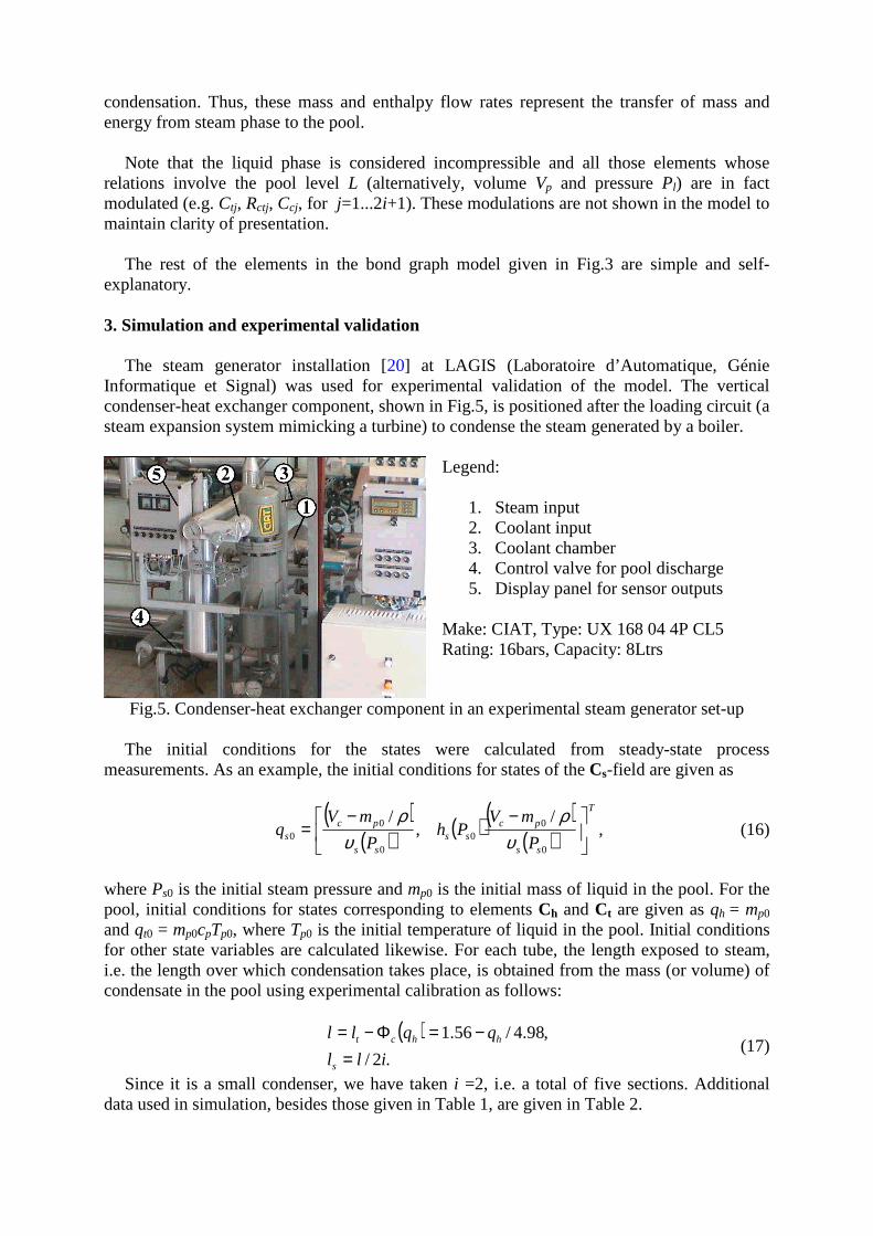
The steam generator installation [20] at LAGIS (Laboratoire d’Automatique, Génie Informatique et Signal) was used for experimental validation of the model. The vertical condenser-heat exchanger component, shown in Fig.5, is positioned after the loading circuit (a steam expansion system mimicking a turbine) to condense the steam generated by a boiler.

Legend: 1. Steam input 2. Coolant input 3. Coolant chamber 4. Control valve for pool discharge 5. Display panel for sensor outputs

Make: CIAT, Type: UX 168 04 4P CL5 Rating: 16bars, Capacity: 8Ltrs

Fig.5. Condenser-heat exchanger component in an experimental steam generator set-up

The initial conditions for the states were calculated from steady-state process measurements. As an example, the initial conditions for states of the Cs-field are given as

( )( ) ( ) ( )

( )T

ss

pcss

ss

pcs P

mVPh

P

mVq

−−=

/ ,

/

0

00

0

00 υ

ρυ

ρ, (16)

where Ps0 is the initial steam pressure and mp0 is the initial mass of liquid in the pool. For the pool, initial conditions for states corresponding to elements Ch and Ct are given as qh = mp0 and qt0 = mp0cpTp0, where Tp0 is the initial temperature of liquid in the pool. Initial conditions for other state variables are calculated likewise. For each tube, the length exposed to steam, i.e. the length over which condensation takes place, is obtained from the mass (or volume) of condensate in the pool using experimental calibration as follows:

( ).2/

,98.4/56.1

ill

qqll

s

hhct

=−=Φ−=

(17)

Since it is a small condenser, we have taken i =2, i.e. a total of five sections. Additional data used in simulation, besides those given in Table 1, are given in Table 2.

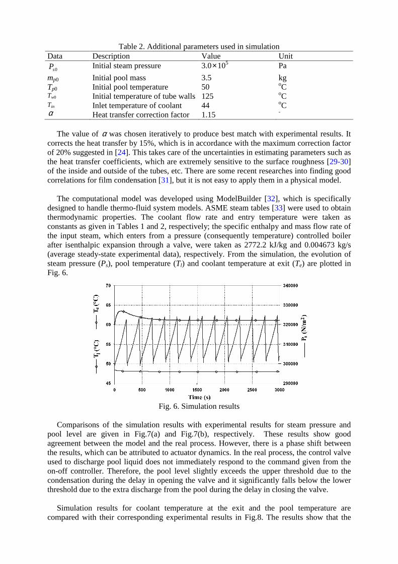
Table 2. Additional parameters used in simulation Data Description Value Unit

0sP Initial steam pressure 3.0×105 Pa

mp0 Initial pool mass 3.5 kg Tp0 Initial pool temperature 50 oC Tw0 Initial temperature of tube walls 125 oC Tin Inlet temperature of coolant 44 oC α Heat transfer correction factor 1.15 -

The value of α was chosen iteratively to produce best match with experimental results. It

corrects the heat transfer by 15%, which is in accordance with the maximum correction factor of 20% suggested in [24]. This takes care of the uncertainties in estimating parameters such as the heat transfer coefficients, which are extremely sensitive to the surface roughness [29-30] of the inside and outside of the tubes, etc. There are some recent researches into finding good correlations for film condensation [31], but it is not easy to apply them in a physical model.

The computational model was developed using ModelBuilder [32], which is specifically designed to handle thermo-fluid system models. ASME steam tables [33] were used to obtain thermodynamic properties. The coolant flow rate and entry temperature were taken as constants as given in Tables 1 and 2, respectively; the specific enthalpy and mass flow rate of the input steam, which enters from a pressure (consequently temperature) controlled boiler after isenthalpic expansion through a valve, were taken as 2772.2 kJ/kg and 0.004673 kg/s (average steady-state experimental data), respectively. From the simulation, the evolution of steam pressure (Ps), pool temperature (Tl) and coolant temperature at exit (Te) are plotted in Fig. 6.

Fig. 6. Simulation results

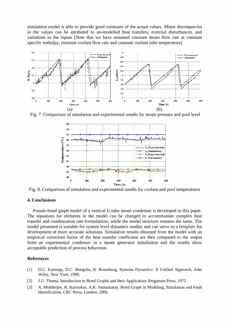
Comparisons of the simulation results with experimental results for steam pressure and

pool level are given in Fig.7(a) and Fig.7(b), respectively. These results show good agreement between the model and the real process. However, there is a phase shift between the results, which can be attributed to actuator dynamics. In the real process, the control valve used to discharge pool liquid does not immediately respond to the command given from the on-off controller. Therefore, the pool level slightly exceeds the upper threshold due to the condensation during the delay in opening the valve and it significantly falls below the lower threshold due to the extra discharge from the pool during the delay in closing the valve.

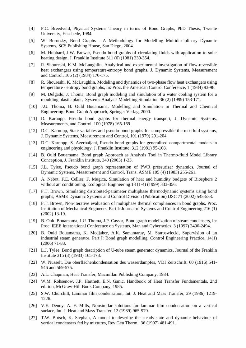
Simulation results for coolant temperature at the exit and the pool temperature are compared with their corresponding experimental results in Fig.8. The results show that the

simulation model is able to provide good estimates of the actual values. Minor discrepancies in the values can be attributed to un-modelled heat transfers, external disturbances, and variations in the inputs (Note that we have assumed constant steam flow rate at constant specific enthalpy, constant coolant flow rate and constant coolant inlet temperature).

(a) (b)

Fig. 7. Comparison of simulation and experimental results for steam pressure and pool level

Fig. 8. Comparison of simulation and experimental results for coolant and pool temperatures

4. Conclusions

Pseudo-bond graph model of a vertical U-tube steam condenser is developed in this paper. The equations for elements in the model can be changed to accommodate complex heat transfer and condensation rate formulations, while the model structure remains the same. The model presented is suitable for system level dynamics studies and can serve as a template for development of more accurate solutions. Simulation results obtained from the model with an empirical correction factor of the heat transfer coefficient are then compared to the output from an experimental condenser in a steam generator installation and the results show acceptable prediction of process behaviour. References

[1] D.C. Karnopp, D.C. Margolis, R. Rosenberg, Systems Dynamics: A Unified Approach, John Wiley, New York, 1990.

[2] J.U. Thoma, Introduction to Bond Graphs and their Application, Pergamon Press, 1975.

[3] A. Mukherjee, R. Karmakar, A.K. Samantaray, Bond Graph in Modeling, Simulation and Fault Identification, CRC Press, London, 2006.

[4] P.C. Breedveld, Physical Systems Theory in terms of Bond Graphs, PhD Thesis, Twente University, Enschede, 1984.

[5] W. Borutzky, Bond Graphs - A Methodology for Modelling Multidisciplinary Dynamic Systems, SCS Publishing House, San Diego, 2004.

[6] M. Hubbard, J.W. Brewer, Pseudo bond graphs of circulating fluids with application to solar heating design, J. Franklin Institute 311 (6) (1981) 339-354.

[7] R. Shoureshi, K.M. McLaughlin, Analytical and experimental investigation of flow-reversible heat exchangers using temperature-entropy bond graphs, J. Dynamic Systems, Measurement and Control, 106 (2) (1984) 170-175.

[8] R. Shoureshi, K. McLaughlin, Modeling and dynamics of two-phase flow heat exchangers using temperature - entropy bond graphs, In: Proc. the American Control Conference, 1 (1984) 93-98.

[9] M. Delgado, J. Thoma, Bond graph modeling and simulation of a water cooling system for a moulding plastic plant, Systems Analysis Modelling Simulation 36 (2) (1999) 153-171.

[10] J.U. Thoma, B. Ould Bouamama, Modelling and Simulation in Thermal and Chemical Engineering: Bond Graph Approach, Springer Verlag, 2000.

[11] D. Karnopp, Pseudo bond graphs for thermal energy transport, J. Dynamic Systems, Measurements, and Control, 100 (1978) 165-169.

[12] D.C. Karnopp, State variables and pseudo-bond graphs for compressible thermo-fluid systems, J. Dynamic Systems, Measurement and Control, 101 (1979) 201-204.

[13] D.C. Karnopp, S. Azerbaijani, Pseudo bond graphs for generalised compartmental models in engineering and physiology, J. Franklin Institute, 312 (1981) 95-108.

[14] B. Ould Bouamama, Bond graph Approach as Analysis Tool in Thermo-fluid Model Library Conception, J. Franklin Institute, 340 (2003) 1-23.

[15] J.L. Tylee, Pseudo bond graph representation of PWR pressurizer dynamics, Journal of Dynamic Systems, Measurement and Control, Trans. ASME 105 (4) (1983) 255-261.

[16] A. Nebot, F.E. Cellier, F. Mugica, Simulation of heat and humidity budgets of Biosphere 2 without air conditioning, Ecological Engineering 13 (1-4) (1999) 333-356.

[17] F.T. Brown, Simulating distributed-parameter multiphase thermodynamic systems using bond graphs, ASME Dynamic Systems and Control Division (Publication) DSC 71 (2002) 545-553.

[18] F.T. Brown, Non-iterative evaluation of multiphase thermal compliances in bond graphs, Proc. Institution of Mechanical Engineers. Part I: Journal of Systems and Control Engineering 216 (1) (2002) 13-19.

[19] B. Ould Bouamama, J.U. Thoma, J.P. Cassar, Bond graph modelization of steam condensers, in: Proc. IEEE International Conference on Systems, Man and Cybernetics, 3 (1997) 2490-2494.

[20] B. Ould Bouamama, K. Medjaher, A.K. Samantaray, M. Staroswiecki, Supervision of an industrial steam generator. Part I: Bond graph modelling, Control Engineering Practice, 14(1) (2006) 71-83.

[21] L.J. Tylee, Bond graph description of U-tube steam generator dynamics, Journal of the Franklin Institute 315 (3) (1983) 165-178.

[22] W. Nusselt, Die oberflächenkondensation des wasserdampfes, VDI Zeitschrift, 60 (1916):541-546 and 569-575.

[23] A.L. Chapman, Heat Transfer, Macmillan Publishing Company, 1984.

[24] W.M. Rohsenow, J.P. Hartnett, E.N. Ganic, Handbook of Heat Transfer Fundamentals, 2nd edition, McGraw-Hill Book Company, 1985.

[25] S.W. Churchill, Laminar film condensation, Int. J. Heat and Mass Transfer, 29 (1986) 1219-1226.

[26] V.E. Denny, A. F. Mills, Nonsimilar solutions for laminar film condensation on a vertical surface, Int. J. Heat and Mass Transfer, 12 (1969) 965-979.

[27] T.W. Botsch, K. Stephan, A model to describe the steady-state and dynamic behaviour of vertical condensers fed by mixtures, Rev Gén Therm., 36 (1997) 481-491.

[28] N. K. Maheshwari, D. Saha, R. K. Sinha, M. Aritomi, Investigation on condensation in presence of a noncondensable gas for a wide range of Reynolds number, Nuclear Engineering and Design, 227 (2004) 219-238.

[29] S.K. Park, M.H. Kim, K.J. Yoo, Effects of a wavy interface on steam-air condensation on a vertical surface, Int. J. Multiphase Flow, 23 (1997) 1031-1042.

[30] S.K. Park, M.H. Kim, K.J. Yoo, Condensation of pure steam and steam-air mixture with surface waves of condensate film on a vertical wall, Int. J. Multiphase Flow, 22 (1996) 893-908.

[31] M. Chun, K. Kim, Assessment of the new and existing correlations for laminar and turbulent film condensations on a vertical surface, Int. Communications in Heat and Mass Transfer, 17 (1990) 431-441.

[32] B. Ould Bouamama, A.K. Samantaray, K. Medjaher, et.al., Model builder using functional and bond graph tools for FDI design, Control Engineering Practice, 13(7) (2005) 875-891.

[33] C.A. Meyer, R.B. McClintock, G.J. Silvestri, R.C. Spencer, ASME steam tables: Thermodynamic and transport properties of steam, 6th edition, ASME, 1993.