Bo ThidØ - cdn. · PDF file“main” 2001/2/27 page 1 Electromagnetic Field...

“main”2001/2/27page 1

ϒ

Bo Thidé

U B

“main”2001/2/27page 2

“main”2001/2/27page 3

ϒELECTROMAGNETIC FIELD THEORY

Bo Thidé

“main”2001/2/27page 4

Also available

ELECTROMAGNETIC FIELD THEORYEXERCISES

by

Tobia Carozzi, Anders Eriksson, Bengt Lundborg,Bo Thidé and Mattias Waldenvik

“main”2001/2/27page 1

ElectromagneticField Theory

Bo Thidé

Swedish Institute of Space Physics

and

Department of Astronomy and Space PhysicsUppsala University, Sweden

ϒU B · C A B · U · S

“main”2001/2/27page 2

This book was typeset in LATEX 2εon an HP9000/700 series workstationand printed on an HP LaserJet 5000GN printer.

Copyright ©1997, 1998, 1999, 2000 and 2001 byBo ThidéUppsala, SwedenAll rights reserved.

Electromagnetic Field TheoryISBN X-XXX-XXXXX-X

“main”2001/2/27page i

Contents

Preface xi

1 Classical Electrodynamics 11.1 Electrostatics . . . . . . . . . . . . . . . . . . . . . . . . . . 1

1.1.1 Coulomb’s law . . . . . . . . . . . . . . . . . . . . . 21.1.2 The electrostatic field . . . . . . . . . . . . . . . . . . 2

1.2 Magnetostatics . . . . . . . . . . . . . . . . . . . . . . . . . 51.2.1 Ampère’s law . . . . . . . . . . . . . . . . . . . . . . 51.2.2 The magnetostatic field . . . . . . . . . . . . . . . . . 6

1.3 Electrodynamics . . . . . . . . . . . . . . . . . . . . . . . . 81.3.1 Equation of continuity for electric charge . . . . . . . 91.3.2 Maxwell’s displacement current . . . . . . . . . . . . 91.3.3 Electromotive force . . . . . . . . . . . . . . . . . . . 101.3.4 Faraday’s law of induction . . . . . . . . . . . . . . . 111.3.5 Maxwell’s microscopic equations . . . . . . . . . . . 141.3.6 Maxwell’s macroscopic equations . . . . . . . . . . . 14

1.4 Electromagnetic Duality . . . . . . . . . . . . . . . . . . . . 15Example 1.1 Faraday’s law as a consequence of conserva-

tion of magnetic charge . . . . . . . . . . . . 16Example 1.2 Duality of the electromagnetodynamic equations 18Example 1.3 Dirac’s symmetrised Maxwell equations for a

fixed mixing angle . . . . . . . . . . . . . . . 18Example 1.4 The complex field six-vector . . . . . . . . 20Example 1.5 Duality expressed in the complex field six-vector 20

Bibliography . . . . . . . . . . . . . . . . . . . . . . . . . . . . . 21

2 Electromagnetic Waves 232.1 The Wave Equations . . . . . . . . . . . . . . . . . . . . . . 24

2.1.1 The wave equation for E . . . . . . . . . . . . . . . . 242.1.2 The wave equation for B . . . . . . . . . . . . . . . . 242.1.3 The time-independent wave equation for E . . . . . . 25

Example 2.1 Wave equations in electromagnetodynamics . 262.2 Plane Waves . . . . . . . . . . . . . . . . . . . . . . . . . . . 28

2.2.1 Telegrapher’s equation . . . . . . . . . . . . . . . . . 292.2.2 Waves in conductive media . . . . . . . . . . . . . . . 30

i

“main”2001/2/27page ii

ii CONTENTS

2.3 Observables and Averages . . . . . . . . . . . . . . . . . . . 32Bibliography . . . . . . . . . . . . . . . . . . . . . . . . . . . . . 33

3 Electromagnetic Potentials 353.1 The Electrostatic Scalar Potential . . . . . . . . . . . . . . . . 353.2 The Magnetostatic Vector Potential . . . . . . . . . . . . . . . 363.3 The Electrodynamic Potentials . . . . . . . . . . . . . . . . . 36

3.3.1 Electrodynamic gauges . . . . . . . . . . . . . . . . . 38Lorentz equations for the electrodynamic potentials . . 38Gauge transformations . . . . . . . . . . . . . . . . . 39

3.3.2 Solution of the Lorentz equations for the electromag-netic potentials . . . . . . . . . . . . . . . . . . . . . 40The retarded potentials . . . . . . . . . . . . . . . . . 43Example 3.1 Electromagnetodynamic potentials . . . . . 44

Bibliography . . . . . . . . . . . . . . . . . . . . . . . . . . . . . 45

4 Relativistic Electrodynamics 474.1 The Special Theory of Relativity . . . . . . . . . . . . . . . . 47

4.1.1 The Lorentz transformation . . . . . . . . . . . . . . 484.1.2 Lorentz space . . . . . . . . . . . . . . . . . . . . . . 49

Radius four-vector in contravariant and covariant form 50Scalar product and norm . . . . . . . . . . . . . . . . 50Metric tensor . . . . . . . . . . . . . . . . . . . . . . 51Invariant line element and proper time . . . . . . . . . 52Four-vector fields . . . . . . . . . . . . . . . . . . . . 54The Lorentz transformation matrix . . . . . . . . . . . 54The Lorentz group . . . . . . . . . . . . . . . . . . . 54

4.1.3 Minkowski space . . . . . . . . . . . . . . . . . . . . 554.2 Covariant Classical Mechanics . . . . . . . . . . . . . . . . . 574.3 Covariant Classical Electrodynamics . . . . . . . . . . . . . . 59

4.3.1 The four-potential . . . . . . . . . . . . . . . . . . . 594.3.2 The Liénard-Wiechert potentials . . . . . . . . . . . . 604.3.3 The electromagnetic field tensor . . . . . . . . . . . . 62

Bibliography . . . . . . . . . . . . . . . . . . . . . . . . . . . . . 65

5 Electromagnetic Fields and Particles 675.1 Charged Particles in an Electromagnetic Field . . . . . . . . . 67

5.1.1 Covariant equations of motion . . . . . . . . . . . . . 67Lagrange formalism . . . . . . . . . . . . . . . . . . 67Hamiltonian formalism . . . . . . . . . . . . . . . . . 70

Downloaded fromhttp://www.plasma.uu.se/CED/Book Draft version released 27th February 2001 at 18:04.

“main”2001/2/27page iii

iii

5.2 Covariant Field Theory . . . . . . . . . . . . . . . . . . . . . 745.2.1 Lagrange-Hamilton formalism for fields and interactions 74

The electromagnetic field . . . . . . . . . . . . . . . . 78Example 5.1 Field energy difference expressed in the field

tensor . . . . . . . . . . . . . . . . . . . . . 79Other fields . . . . . . . . . . . . . . . . . . . . . . . 82

Bibliography . . . . . . . . . . . . . . . . . . . . . . . . . . . . . 83

6 Electromagnetic Fields and Matter 856.1 Electric Polarisation and Displacement . . . . . . . . . . . . . 85

6.1.1 Electric multipole moments . . . . . . . . . . . . . . 856.2 Magnetisation and the Magnetising Field . . . . . . . . . . . . 886.3 Energy and Momentum . . . . . . . . . . . . . . . . . . . . . 90

6.3.1 The energy theorem in Maxwell’s theory . . . . . . . 906.3.2 The momentum theorem in Maxwell’s theory . . . . . 91

Bibliography . . . . . . . . . . . . . . . . . . . . . . . . . . . . . 93

7 Electromagnetic Fields from Arbitrary Source Distributions 957.1 The Magnetic Field . . . . . . . . . . . . . . . . . . . . . . . 977.2 The Electric Field . . . . . . . . . . . . . . . . . . . . . . . . 997.3 The Radiation Fields . . . . . . . . . . . . . . . . . . . . . . 1017.4 Radiated Energy . . . . . . . . . . . . . . . . . . . . . . . . . 104

7.4.1 Monochromatic signals . . . . . . . . . . . . . . . . . 1047.4.2 Finite bandwidth signals . . . . . . . . . . . . . . . . 104

Bibliography . . . . . . . . . . . . . . . . . . . . . . . . . . . . . 106

8 Electromagnetic Radiation and Radiating Systems 1078.1 Radiation from Extended Sources . . . . . . . . . . . . . . . 107

8.1.1 Radiation from a one-dimensional current distribution 1088.1.2 Radiation from a two-dimensional current distribution 109

8.2 Multipole Radiation . . . . . . . . . . . . . . . . . . . . . . . 1138.2.1 The Hertz potential . . . . . . . . . . . . . . . . . . . 1138.2.2 Electric dipole radiation . . . . . . . . . . . . . . . . 1178.2.3 Magnetic dipole radiation . . . . . . . . . . . . . . . 1188.2.4 Electric quadrupole radiation . . . . . . . . . . . . . . 119

8.3 Radiation from a Localised Charge in Arbitrary Motion . . . . 1208.3.1 The Liénard-Wiechert potentials . . . . . . . . . . . . 1218.3.2 Radiation from an accelerated point charge . . . . . . 123

The differential operator method . . . . . . . . . . . . 125Example 8.1 The fields from a uniformly moving charge . 130

Draft version released 27th February 2001 at 18:04. Downloaded fromhttp://www.plasma.uu.se/CED/Book

“main”2001/2/27page iv

iv CONTENTS

Example 8.2 The convection potential and the convectionforce . . . . . . . . . . . . . . . . . . . . . 132

Radiation for small velocities . . . . . . . . . . . . . 1358.3.3 Bremsstrahlung . . . . . . . . . . . . . . . . . . . . . 136

Example 8.3 Bremsstrahlung for low speeds and short ac-celeration times . . . . . . . . . . . . . . . . 139

8.3.4 Cyclotron and synchrotron radiation . . . . . . . . . . 141Cyclotron radiation . . . . . . . . . . . . . . . . . . . 143Synchrotron radiation . . . . . . . . . . . . . . . . . . 144Radiation in the general case . . . . . . . . . . . . . . 146Virtual photons . . . . . . . . . . . . . . . . . . . . . 147

8.3.5 Radiation from charges moving in matter . . . . . . . 149Vavilov-Cerenkov radiation . . . . . . . . . . . . . . 151

Bibliography . . . . . . . . . . . . . . . . . . . . . . . . . . . . . 156

F Formulae 157F.1 The Electromagnetic Field . . . . . . . . . . . . . . . . . . . 157

F.1.1 Maxwell’s equations . . . . . . . . . . . . . . . . . . 157Constitutive relations . . . . . . . . . . . . . . . . . . 157

F.1.2 Fields and potentials . . . . . . . . . . . . . . . . . . 157Vector and scalar potentials . . . . . . . . . . . . . . 157Lorentz’ gauge condition in vacuum . . . . . . . . . . 158

F.1.3 Force and energy . . . . . . . . . . . . . . . . . . . . 158Poynting’s vector . . . . . . . . . . . . . . . . . . . . 158Maxwell’s stress tensor . . . . . . . . . . . . . . . . . 158

F.2 Electromagnetic Radiation . . . . . . . . . . . . . . . . . . . 158F.2.1 Relationship between the field vectors in a plane wave 158F.2.2 The far fields from an extended source distribution . . 158F.2.3 The far fields from an electric dipole . . . . . . . . . . 158F.2.4 The far fields from a magnetic dipole . . . . . . . . . 159F.2.5 The far fields from an electric quadrupole . . . . . . . 159F.2.6 The fields from a point charge in arbitrary motion . . . 159F.2.7 The fields from a point charge in uniform motion . . . 159

F.3 Special Relativity . . . . . . . . . . . . . . . . . . . . . . . . 160F.3.1 Metric tensor . . . . . . . . . . . . . . . . . . . . . . 160F.3.2 Covariant and contravariant four-vectors . . . . . . . . 160F.3.3 Lorentz transformation of a four-vector . . . . . . . . 160F.3.4 Invariant line element . . . . . . . . . . . . . . . . . . 160F.3.5 Four-velocity . . . . . . . . . . . . . . . . . . . . . . 160F.3.6 Four-momentum . . . . . . . . . . . . . . . . . . . . 160


“main”2001/2/27page v

v

F.3.7 Four-current density . . . . . . . . . . . . . . . . . . 161F.3.8 Four-potential . . . . . . . . . . . . . . . . . . . . . . 161F.3.9 Field tensor . . . . . . . . . . . . . . . . . . . . . . . 161

F.4 Vector Relations . . . . . . . . . . . . . . . . . . . . . . . . . 161F.4.1 Spherical polar coordinates . . . . . . . . . . . . . . . 161

Base vectors . . . . . . . . . . . . . . . . . . . . . . 161Directed line element . . . . . . . . . . . . . . . . . . 162Solid angle element . . . . . . . . . . . . . . . . . . . 162Directed area element . . . . . . . . . . . . . . . . . 162Volume element . . . . . . . . . . . . . . . . . . . . 162

F.4.2 Vector formulae . . . . . . . . . . . . . . . . . . . . . 162General vector algebraic identities . . . . . . . . . . . 162General vector analytic identities . . . . . . . . . . . . 163Special identities . . . . . . . . . . . . . . . . . . . . 163Integral relations . . . . . . . . . . . . . . . . . . . . 163

Bibliography . . . . . . . . . . . . . . . . . . . . . . . . . . . . . 164

Appendices 157

M Mathematical Methods 165M.1 Scalars, Vectors and Tensors . . . . . . . . . . . . . . . . . . 165

M.1.1 Vectors . . . . . . . . . . . . . . . . . . . . . . . . . 165Radius vector . . . . . . . . . . . . . . . . . . . . . . 165

M.1.2 Fields . . . . . . . . . . . . . . . . . . . . . . . . . . 167Scalar fields . . . . . . . . . . . . . . . . . . . . . . . 167Vector fields . . . . . . . . . . . . . . . . . . . . . . 167Tensor fields . . . . . . . . . . . . . . . . . . . . . . 168Example M.1 Tensors in 3D space . . . . . . . . . . . . 170

M.1.3 Vector algebra . . . . . . . . . . . . . . . . . . . . . 173Scalar product . . . . . . . . . . . . . . . . . . . . . 173Example M.2 Inner products in complex vector space . . . 173Example M.3 Scalar product, norm and metric in Lorentz

space . . . . . . . . . . . . . . . . . . . . . 174Example M.4 Metric in general relativity . . . . . . . . . 174Dyadic product . . . . . . . . . . . . . . . . . . . . . 175Vector product . . . . . . . . . . . . . . . . . . . . . 176

M.1.4 Vector analysis . . . . . . . . . . . . . . . . . . . . . 176The del operator . . . . . . . . . . . . . . . . . . . . 176Example M.5 The four-del operator in Lorentz space . . . 177The gradient . . . . . . . . . . . . . . . . . . . . . . 178


“main”2001/2/27page vi

vi CONTENTS

Example M.6 Gradients of scalar functions of relative dis-tances in 3D . . . . . . . . . . . . . . . . . . 178

The divergence . . . . . . . . . . . . . . . . . . . . . 179Example M.7 Divergence in 3D . . . . . . . . . . . . . 179The Laplacian . . . . . . . . . . . . . . . . . . . . . . 179Example M.8 The Laplacian and the Dirac delta . . . . . 179The curl . . . . . . . . . . . . . . . . . . . . . . . . . 180Example M.9 The curl of a gradient . . . . . . . . . . . 180Example M.10 The divergence of a curl . . . . . . . . . 181

M.2 Analytical Mechanics . . . . . . . . . . . . . . . . . . . . . . 182M.2.1 Lagrange’s equations . . . . . . . . . . . . . . . . . . 182M.2.2 Hamilton’s equations . . . . . . . . . . . . . . . . . . 182

Bibliography . . . . . . . . . . . . . . . . . . . . . . . . . . . . . 183


“main”2001/2/27page vii

List of Figures

1.1 Coulomb interaction . . . . . . . . . . . . . . . . . . . . . . 31.2 Ampère interaction . . . . . . . . . . . . . . . . . . . . . . . 61.3 Moving loop in a varying B field . . . . . . . . . . . . . . . . 12

4.1 Relative motion of two inertial systems . . . . . . . . . . . . 484.2 Rotation in a 2D Euclidean space . . . . . . . . . . . . . . . . 554.3 Minkowski diagram . . . . . . . . . . . . . . . . . . . . . . . 56

5.1 Linear one-dimensional mass chain . . . . . . . . . . . . . . . 74

7.1 Radiation in the far zone . . . . . . . . . . . . . . . . . . . . 103

8.1 Loop antenna . . . . . . . . . . . . . . . . . . . . . . . . . . 1108.2 Radiation from a moving charge in vacuum . . . . . . . . . . 1218.3 An accelerated charge in vacuum . . . . . . . . . . . . . . . . 1248.4 Angular distribution of radiation during bremsstrahlung . . . . 1378.5 Location of radiation during bremsstrahlung . . . . . . . . . . 1388.6 Radiation from a charge in circular motion . . . . . . . . . . . 1428.7 Synchrotron radiation lobe width . . . . . . . . . . . . . . . . 1448.8 The perpendicular field of a moving charge . . . . . . . . . . 1478.9 Vavilov-Cerenkov cone . . . . . . . . . . . . . . . . . . . . . 153

M.1 Surface element of a material body . . . . . . . . . . . . . . . 170M.2 Tetrahedron-like volume element of matter . . . . . . . . . . . 171

vii

“main”2001/2/27page viii

“main”2001/2/27page ix

To the memory of professorLEV MIKHAILOVICH ERUKHIMOV

dear friend, remarkable physicistand a truly great human being.

“main”2001/2/27page x

If you understand, things are such as they areIf you do not understand, things are such as they are

GENSHA

“main”2001/2/27page xi

Preface

This book is the result of a twenty-five year long love affair. In 1972, I tookmy first advanced course in electrodynamics at the Theoretical Physics depart-ment, Uppsala University. Shortly thereafter, I joined the research group thereand took on the task of helping my supervisor, professor PER-OLOF FRÖ-MAN, with the preparation of a new version of his lecture notes on ElectricityTheory. These two things opened up my eyes for the beauty and intricacy ofelectrodynamics, already at the classical level, and I fell in love with it.

Ever since that time, I have off and on had reason to return to electrody-namics, both in my studies, research and teaching, and the current book is theresult of my own teaching of a course in advanced electrodynamics at UppsalaUniversity some twenty odd years after I experienced the first encounter withthis subject. The book is the outgrowth of the lecture notes that I preparedfor the four-credit course Electrodynamics that was introduced in the Upp-sala University curriculum in 1992, to become the five-credit course ClassicalElectrodynamics in 1997. To some extent, parts of these notes were based onlecture notes prepared, in Swedish, by BENGT LUNDBORG who created, de-veloped and taught the earlier, two-credit course Electromagnetic Radiation atour faculty.

Intended primarily as a textbook for physics students at the advanced un-dergraduate or beginning graduate level, I hope the book may be useful forresearch workers too. It provides a thorough treatment of the theory of elec-trodynamics, mainly from a classical field theoretical point of view, and in-cludes such things as electrostatics and magnetostatics and their unificationinto electrodynamics, the electromagnetic potentials, gauge transformations,covariant formulation of classical electrodynamics, force, momentum and en-ergy of the electromagnetic field, radiation and scattering phenomena, electro-magnetic waves and their propagation in vacuum and in media, and covariantLagrangian/Hamiltonian field theoretical methods for electromagnetic fields,particles and interactions. The aim has been to write a book that can serveboth as an advanced text in Classical Electrodynamics and as a preparation forstudies in Quantum Electrodynamics and related subjects.

In an attempt to encourage participation by other scientists and students inthe authoring of this book, and to ensure its quality and scope to make it usefulin higher university education anywhere in the world, it was produced withina World-Wide Web (WWW) project. This turned out to be a rather successful

xi

“main”2001/2/27page xii

xii PREFACE

move. By making an electronic version of the book freely down-loadable onthe net, I have not only received comments on it from fellow Internet physicistsaround the world, but know, from WWW ‘hit’ statistics that at the time ofwriting this, the book serves as a frequently used Internet resource. This wayit is my hope that it will be particularly useful for students and researchersworking under financial or other circumstances that make it difficult to procurea printed copy of the book.

I am grateful not only to Per-Olof Fröman and Bengt Lundborg for provid-ing the inspiration for my writing this book, but also to CHRISTER WAHLBERG

and GÖRAN FÄLDT, Uppsala University, and YAKOV ISTOMIN, Lebedev In-stitute, Moscow, for interesting discussions on electrodynamics and relativityin general and on this book in particular. I also wish to thank my formergraduate students MATTIAS WALDENVIK and TOBIA CAROZZI as well asANDERS ERIKSSON, all at the Swedish Institute of Space Physics, UppsalaDivision, who all have participated in the teaching and commented on the ma-terial covered in the course and in this book. Thanks are also due to my long-term space physics colleague HELMUT KOPKA of the Max-Planck-Institut fürAeronomie, Lindau, Germany, who not only taught me about the practical as-pects of the of high-power radio wave transmitters and transmission lines, butalso about the more delicate aspects of typesetting a book in TEX and LATEX.I am particularly indebted to Academician professor VITALIY L. GINZBURG

for his many fascinating and very elucidating lectures, comments and histor-ical footnotes on electromagnetic radiation while cruising on the Volga riverduring our joint Russian-Swedish summer schools.

Finally, I would like to thank all students and Internet users who havedownloaded and commented on the book during its life on the World-WideWeb.

I dedicate this book to my son MATTIAS, my daughter KAROLINA, myhigh-school physics teacher, STAFFAN RÖSBY, and to my fellow members ofthe CAPELLA PEDAGOGICA UPSALIENSIS.

Uppsala, Sweden BO THIDÉ

February, 2001


“main”2001/2/27page 1

1Classical

Electrodynamics

Classical electrodynamics deals with electric and magnetic fields and inter-actions caused by macroscopic distributions of electric charges and currents.This means that the concepts of localised electric charges and currents assumethe validity of certain mathematical limiting processes in which it is consideredpossible for the charge and current distributions to be localised in infinitesi-mally small volumes of space. Clearly, this is in contradiction to electromag-netism on a truly microscopic scale, where charges and currents are known tobe spatially extended objects. However, the limiting processes used will yieldresults which are correct on small as well as large macroscopic scales.

In this chapter we start with the force interactions in classical electrostat-ics and classical magnetostatics and introduce the static electric and magneticfields and find two uncoupled systems of equations for them. Then we see howthe conservation of electric charge and its relation to electric current leads tothe dynamic connection between electricity and magnetism and how the twocan be unified in one theory, classical electrodynamics, described by one sys-tem of coupled dynamic field equations—the Maxwell equations.

At the end of the chapter we study Dirac’s symmetrised form of Maxwell’sequations by introducing (hypothetical) magnetic charges and magnetic cur-rents into the theory. While not identified unambiguously in experiments yet,magnetic charges and currents make the theory much more appealing for in-stance by allowing for duality transformations in a most natural way.

1.1 ElectrostaticsThe theory which describes physical phenomena related to the interaction be-tween stationary electric charges or charge distributions in space is called elec-trostatics.1 For a long time electrostatics was considered an independent phys-

1The famous physicist and philosopher Pierre Duhem (1861–1916) once wrote:

1

“main”2001/2/27page 2

2 CLASSICAL ELECTRODYNAMICS

ical theory of its own, alongside other physical theories such as mechanics andthermodynamics.

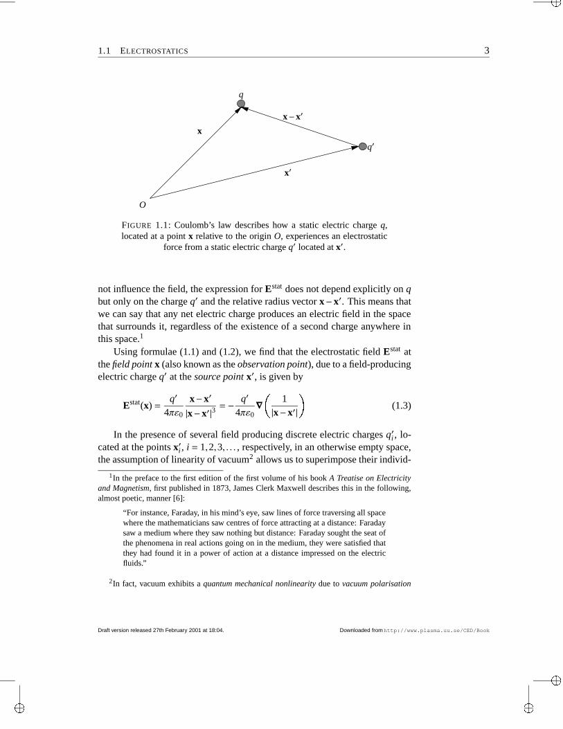
1.1.1 Coulomb’s lawIt has been found experimentally that in classical electrostatics the interactionbetween two stationary electrically charged bodies can be described in terms ofa mechanical force. Let us consider the simple case described by Figure 1.1 onthe facing page. Let F denote the force acting on a electrically charged particlewith charge q located at x, due to the presence of a charge q′ located at x′.According to Coulomb’s law this force is, in vacuum, given by the expression

F(x) =qq′

4πε0

x−x′

|x−x′|3 = − qq′

4πε0∇ 1|x−x′| (1.1)

where we have used results from Example M.6 on page 178. In SI units, whichwe shall use throughout, the force F is measured in Newton (N), the electriccharges q and q′ in Coulomb (C) [= Ampère-seconds (As)], and the length|x−x′| in metres (m). The constant ε0 = 107/(4πc2) ≈ 8.8542× 10−12 Faradper metre (F/m) is the vacuum permittivity and c ≈ 2.9979× 108 m/s is thespeed of light in vacuum. In CGS units ε0 = 1/(4π) and the force is measuredin dyne, electric charge in statcoulomb, and length in centimetres (cm).

1.1.2 The electrostatic fieldInstead of describing the electrostatic interaction in terms of a “force actionat a distance,” it turns out that it is often more convenient to introduce theconcept of a field and to describe the electrostatic interaction in terms of astatic vectorial electric field Estat defined by the limiting process

Estat def≡ limq→0

Fq

(1.2)

where F is the electrostatic force, as defined in Equation (1.1), from a netelectric charge q′ on the test particle with a small electric net electric charge q.Since the purpose of the limiting process is to assure that the test charge q does

“The whole theory of electrostatics constitutes a group of abstract ideas andgeneral propositions, formulated in the clear and concise language of geometryand algebra, and connected with one another by the rules of strict logic. Thiswhole fully satisfies the reason of a French physicist and his taste for clarity,simplicity and order. . . ”


“main”2001/2/27page 3

1.1 ELECTROSTATICS 3

O

x′

x

q

x−x′

q′

FIGURE 1.1: Coulomb’s law describes how a static electric charge q,located at a point x relative to the origin O, experiences an electrostatic

force from a static electric charge q′ located at x′.

not influence the field, the expression for Estat does not depend explicitly on qbut only on the charge q′ and the relative radius vector x−x′. This means thatwe can say that any net electric charge produces an electric field in the spacethat surrounds it, regardless of the existence of a second charge anywhere inthis space.1

Using formulae (1.1) and (1.2), we find that the electrostatic field Estat atthe field point x (also known as the observation point), due to a field-producingelectric charge q′ at the source point x′, is given by

Estat(x) =q′

4πε0

x−x′

|x−x′|3 = − q′

4πε0∇ 1|x−x′| (1.3)

In the presence of several field producing discrete electric charges q′i , lo-cated at the points x′i , i = 1,2,3, . . . , respectively, in an otherwise empty space,the assumption of linearity of vacuum2 allows us to superimpose their individ-

1In the preface to the first edition of the first volume of his book A Treatise on Electricityand Magnetism, first published in 1873, James Clerk Maxwell describes this in the following,almost poetic, manner [6]:

“For instance, Faraday, in his mind’s eye, saw lines of force traversing all spacewhere the mathematicians saw centres of force attracting at a distance: Faradaysaw a medium where they saw nothing but distance: Faraday sought the seat ofthe phenomena in real actions going on in the medium, they were satisfied thatthey had found it in a power of action at a distance impressed on the electricfluids.”

2In fact, vacuum exhibits a quantum mechanical nonlinearity due to vacuum polarisation


“main”2001/2/27page 4


ual E fields into a total E field

Estat(x) =1

4πε0∑

iq′i

x−x′i x−x′i 3 (1.4)

If the discrete electric charges are small and numerous enough, we intro-duce the electric charge density ρ located at x′ and write the total field as

Estat(x) =1

4πε0 Vρ(x′)

x−x′

|x−x′|3 d3x′ =− 14πε0 V

ρ(x′)∇ 1|x−x′| d3x′ (1.5)

where, in the last step, we used formula Equation (M.68) on page 178. Weemphasise that Equation (1.5) above is valid for an arbitrary distribution ofelectric charges, including discrete charges, in which case ρ can be expressedin terms of one or more Dirac delta distributions. Since, according to for-mula Equation (M.78) on page 181, ∇× [∇α(x)] ≡ 0 for any 3D 3 scalar fieldα(x), we immediately find that in electrostatics

∇×Estat(x) = − 14πε0

∇× Vρ(x′) ∇ 1

|x−x′| d3x′

= − 14πε0 V

ρ(x′)∇× ∇ 1|x−x′| d3x′

= 0

(1.6)

I.e., Estat is an irrotational field.Taking the divergence of the general Estat expression for an arbitrary elec-

tric charge distribution, Equation (1.5), and using the representation of theDirac delta distribution, Equation (M.73) on page 180, we find that

∇ ·Estat(x) = ∇ · 14πε0 V

ρ(x′)x−x′

|x−x′|3 d3x′

= − 14πε0 V

ρ(x′)∇ ·∇ 1|x−x′| d3x′

= − 14πε0 V

ρ(x′)∇2 1|x−x′| d3x′

=1ε0 V

ρ(x′)δ(x−x′)d3x′

=ρ(x)ε0

(1.7)

which is Gauss’s law in differential form.

effects manifesting themselves in the momentary creation and annihilation of electron-positronpairs, but classically this nonlinearity is negligible.


“main”2001/2/27page 5

1.2 MAGNETOSTATICS 5

1.2 MagnetostaticsWhile electrostatics deals with static electric charges, magnetostatics dealswith stationary electric currents, i.e., electric charges moving with constantspeeds, and the interaction between these currents. Let us discuss this theoryin some detail.

1.2.1 Ampère’s lawExperiments on the interaction between two small loops of electric currenthave shown that they interact via a mechanical force, much the same way thatelectric charges interact. Let F denote such a force acting on a small loop Ccarrying a current J located at x, due to the presence of a small loop C ′ carryinga current J′ located at x′. According to Ampère’s law this force is, in vacuum,given by the expression

F(x) =µ0JJ′

4π C C′dl× dl′× (x−x′)

|x−x′|3

= −µ0JJ′

4π C C′dl× dl′×∇ 1

|x−x′| (1.8)

Here dl and dl′ are tangential line elements of the loops C and C′, respectively,and, in SI units, µ0 = 4π×10−7 ≈ 1.2566×10−6 H/m is the vacuum permeabil-ity. From the definition of ε0 and µ0 (in SI units) we observe that

ε0µ0 =107

4πc2 (F/m) ×4π×10−7 (H/m) =1c2 (s2/m2) (1.9)

which is a useful relation.At first glance, Equation (1.8) above may appear unsymmetric in terms

of the loops and therefore to be a force law which is in contradiction withNewton’s third law. However, by applying the vector triple product “bac-cab”Formula (F.54) on page 162, we can rewrite (1.8) as

F(x) = −µ0JJ′

4π C C′ dl ·∇ 1

|x−x′| dl′

− µ0JJ′

4π C C′

x−x′

|x−x′|3 dl ·dl′(1.10)

Recognising the fact that the integrand in the first integral is an exact differen-tial so that this integral vanishes, we can rewrite the force expression, Equa-tion (1.8) above, in the following symmetric way

F(x) = −µ0JJ′

4π C C′

x−x′

|x−x′|3 dl ·dl′ (1.11)


“main”2001/2/27page 6


O

dlC

J

J′C′

x−x′

x

dl′

x′

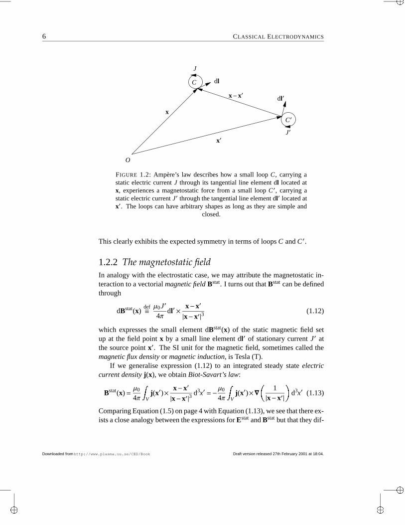
FIGURE 1.2: Ampère’s law describes how a small loop C, carrying astatic electric current J through its tangential line element dl located atx, experiences a magnetostatic force from a small loop C′, carrying astatic electric current J′ through the tangential line element dl′ located atx′. The loops can have arbitrary shapes as long as they are simple and

closed.

This clearly exhibits the expected symmetry in terms of loops C and C ′.

1.2.2 The magnetostatic fieldIn analogy with the electrostatic case, we may attribute the magnetostatic in-teraction to a vectorial magnetic field Bstat. I turns out that Bstat can be definedthrough

dBstat(x)def≡ µ0J′

4πdl′× x−x′

|x−x′|3 (1.12)

which expresses the small element dBstat(x) of the static magnetic field setup at the field point x by a small line element dl′ of stationary current J′ atthe source point x′. The SI unit for the magnetic field, sometimes called themagnetic flux density or magnetic induction, is Tesla (T).

If we generalise expression (1.12) to an integrated steady state electriccurrent density j(x), we obtain Biot-Savart’s law:

Bstat(x) =µ0

4π Vj(x′)× x−x′

|x−x′|3 d3x′ =−µ0

4π Vj(x′)×∇ 1

|x−x′| d3x′ (1.13)

Comparing Equation (1.5) on page 4 with Equation (1.13), we see that there ex-ists a close analogy between the expressions for Estat and Bstat but that they dif-


“main”2001/2/27page 7

1.2 MAGNETOSTATICS 7

fer in their vectorial characteristics. With this definition of Bstat, Equation (1.8)on page 5 may we written

F(x) = J Cdl×Bstat(x) (1.14)

In order to assess the properties of Bstat, we determine its divergence andcurl. Taking the divergence of both sides of Equation (1.13) on the facing pageand utilising Formula (F.61) on page 163, we obtain

∇ ·Bstat(x) = −µ0

4π∇ · V

j(x′)×∇ 1|x−x′| d3x′

= −µ0

4π V∇ 1|x−x′| · [∇× j(x′)]d3x′

+µ0

4π Vj(x′) · ∇×∇ 1

|x−x′| d3x′

= 0

(1.15)

where the first term vanishes because j(x′) is independent of x so that ∇×j(x′) ≡ 0, and the second term vanishes since, according to Equation (M.78) onpage 181, ∇× [∇α(x)] vanishes for any scalar field α(x).

Applying the operator “bac-cab” rule, Formula (F.67) on page 163, the curlof Equation (1.13) on the preceding page can be written

∇×Bstat(x) = −µ0

4π∇× V

j(x′)×∇ 1|x−x′| d3x′

= −µ0

4π Vj(x′)∇2 1

|x−x′| d3x′

+µ0

4π V[j(x′) ·∇′]∇′ 1

|x−x′| d3x′

(1.16)

In the first of the two integrals on the right hand side, we use the representationof the Dirac delta function Equation (M.73) on page 180, and integrate thesecond one by parts, by utilising Formula (F.59) on page 163 as follows:

V[j(x′) ·∇′]∇′ 1

|x−x′| d3x′

= xk V∇′ · j(x′) ∂

∂x′k 1|x−x′| d3x′− V ∇′ · j(x′) ∇′ 1

|x−x′| d3x′

= xk Sj(x′)

∂

∂x′k 1|x−x′| ·dS− V ∇′ · j(x′) ∇′ 1

|x−x′| d3x′


“main”2001/2/27page 8


(1.17)

Then we note that the first integral in the result, obtained by applying Gauss’stheorem, vanishes when integrated over a large sphere far away from the lo-calised source j(x′), and that the second integral vanishes because ∇ · j = 0 forstationary currents (no charge accumulation in space). The net result is simply

∇×Bstat(x) = µ0 Vj(x′)δ(x−x′)d3x′ = µ0j(x) (1.18)

1.3 ElectrodynamicsAs we saw in the previous sections, the laws of electrostatics and magneto-statics can be summarised in two pairs of time-independent, uncoupled vectordifferential equations, namely the equations of classical electrostatics

∇ ·Estat(x) =ρ(x)ε0

(1.19a)

∇×Estat(x) = 0 (1.19b)

and the equations of classical magnetostatics

∇ ·Bstat(x) = 0 (1.20a)

∇×Bstat(x) = µ0j(x) (1.20b)

Since there is nothing a priori which connects Estat directly with Bstat, we mustconsider classical electrostatics and classical magnetostatics as two indepen-dent theories.

However, when we include time-dependence, these theories are unifiedinto one theory, classical electrodynamics. This unification of the theories ofelectricity and magnetism is motivated by two empirically established facts:

1. Electric charge is a conserved quantity and electric current is a transportof electric charge. This fact manifests itself in the equation of continuityand, as a consequence, in Maxwell’s displacement current.

2. A change in the magnetic flux through a loop will induce an EMF elec-tric field in the loop. This is the celebrated Faraday’s law of induction.


“main”2001/2/27page 9

1.3 ELECTRODYNAMICS 9

1.3.1 Equation of continuity for electric chargeLet j denote the electric current density (measured in A/m2). In the simplestcase it can be defined as j = vρ where v is the velocity of the electric chargedensity ρ. In general, j has to be defined in statistical mechanical terms asj(t,x) = ∑α qe

α v fα(t,x,v)d3v where fα(t,x,v) is the (normalised) distributionfunction for particle species α with electric charge qe

α.The electric charge conservation law can be formulated in the equation of

continuity

∂ρ(t,x)∂t

+∇ · j(t,x) = 0 (1.21)

which states that the time rate of change of electric charge ρ(t,x) is balancedby a divergence in the electric current density j(t,x).

1.3.2 Maxwell’s displacement currentWe recall from the derivation of Equation (1.18) on the preceding page thatthere we used the fact that in magnetostatics ∇ · j(x) = 0. In the case of non-stationary sources and fields, we must, in accordance with the continuity Equa-tion (1.21), set ∇ · j(t,x) = −∂ρ(t,x)/∂t. Doing so, and formally repeating thesteps in the derivation of Equation (1.18) on the preceding page, we wouldobtain the formal result

∇×B(t,x) = µ0 Vj(t,x′)δ(x−x′)d3x′+

µ0

4π∂

∂t Vρ(t,x′)∇′ 1

|x−x′| d3x′

= µ0j(t,x) +µ0∂

∂tε0E(t,x)

(1.22)

where, in the last step, we have assumed that a generalisation of Equation (1.5)on page 4 to time-varying fields allows us to make the identification

14πε0

∂

∂t Vρ(t,x′)∇′ 1

|x−x′| d3x′ =∂

∂t − 1

4πε0 Vρ(t,x′)∇ 1

|x−x′| d3x′ =∂

∂tE(t,x)

(1.23)

Later, we will need to consider this formal result further. The result is Maxwell’ssource equation for the B field

∇×B(t,x) = µ0 j(t,x) +∂

∂tε0E(t,x) (1.24)


“main”2001/2/27page 10


where the last term ∂ε0E(t,x)/∂t is the famous displacement current. Thisterm was introduced, in a stroke of genius, by Maxwell in order to make theright hand side of this equation divergence free when j(t,x) is assumed to rep-resent the density of the total electric current, which can be split up in “or-dinary” conduction currents, polarisation currents and magnetisation currents.The displacement current is an extra term which behaves like a current densityflowing in vacuum. As we shall see later, its existence has far-reaching physi-cal consequences as it predicts the existence of electromagnetic radiation thatcan carry energy and momentum over very long distances, even in vacuum.

1.3.3 Electromotive forceIf an electric field E(t,x) is applied to a conducting medium, a current densityj(t,x) will be produced in this medium. There exist also hydrodynamical andchemical processes which can create currents. Under certain physical condi-tions, and for certain materials, one can sometimes assume a linear relationshipbetween the electric current density j and E, called Ohm’s law:

j(t,x) = σE(t,x) (1.25)

where σ is the electric conductivity (S/m). In the most general cases, for in-stance in an anisotropic conductor, σ is a tensor.

We can view Ohm’s law, Equation (1.25) above, as the first term in a Taylorexpansion of the law j[E(t,x)]. This general law incorporates non-linear effectssuch as frequency mixing. Examples of media which are highly non-linear aresemiconductors and plasma. We draw the attention to the fact that even in caseswhen the linear relation between E and j is a good approximation, we still haveto use Ohm’s law with care. The conductivity σ is, in general, time-dependent(temporal dispersive media) but then it is often the case that Equation (1.25) isvalid for each individual Fourier component of the field.

If the current is caused by an applied electric field E(t,x), this electric fieldwill exert work on the charges in the medium and, unless the medium is super-conducting, there will be some energy loss. The rate at which this energy isexpended is j ·E per unit volume. If E is irrotational (conservative), j willdecay away with time. Stationary currents therefore require that an electricfield which corresponds to an electromotive force (EMF) is present. In thepresence of such a field EEMF, Ohm’s law, Equation (1.25) above, takes theform

j = σ(Estat + EEMF) (1.26)


“main”2001/2/27page 11


The electromotive force is defined as

E = C(Estat + EEMF) ·dl (1.27)

where dl is a tangential line element of the closed loop C.

1.3.4 Faraday’s law of inductionIn Subsection 1.1.2 we derived the differential equations for the electrostaticfield. In particular, on page 4 we derived Equation (1.6) which states that∇×Estat(x) = 0 and thus that Estat is a conservative field (it can be expressedas a gradient of a scalar field). This implies that the closed line integral of Estat

in Equation (1.27) above vanishes and that this equation becomes

E = CEEMF ·dl (1.28)

It has been established experimentally that a nonconservative EMF field isproduced in a closed circuit C if the magnetic flux through this circuit varieswith time. This is formulated in Faraday’s law which, in Maxwell’s gener-alised form, reads

E(t,x) = CE(t,x) ·dl = − d

dtΦm(t,x)

= − ddt S

B(t,x) ·dS = − SdS · ∂

∂tB(t,x)

(1.29)

where Φm is the magnetic flux and S is the surface encircled by C which can beinterpreted as a generic stationary “loop” and not necessarily as a conductingcircuit. Application of Stokes’ theorem on this integral equation, transforms itinto the differential equation

∇×E(t,x) = − ∂∂t

B(t,x) (1.30)

which is valid for arbitrary variations in the fields and constitutes the Maxwellequation which explicitly connects electricity with magnetism.

Any change of the magnetic flux Φm will induce an EMF. Let us thereforeconsider the case, illustrated if Figure 1.3.4 on the following page, that the“loop” is moved in such a way that it links a magnetic field which varies duringthe movement. The convective derivative is evaluated according to the well-known operator formula


“main”2001/2/27page 12


B(x)

dSv

v

dl

C

B(x)

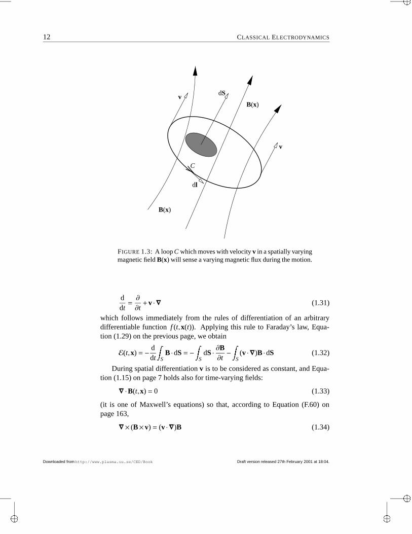
FIGURE 1.3: A loop C which moves with velocity v in a spatially varyingmagnetic field B(x) will sense a varying magnetic flux during the motion.

ddt

=∂

∂t+ v ·∇ (1.31)

which follows immediately from the rules of differentiation of an arbitrarydifferentiable function f (t,x(t)). Applying this rule to Faraday’s law, Equa-tion (1.29) on the previous page, we obtain

E(t,x) = − ddt S

B ·dS = − SdS · ∂B

∂t− S

(v ·∇)B ·dS (1.32)

During spatial differentiation v is to be considered as constant, and Equa-tion (1.15) on page 7 holds also for time-varying fields:

∇ ·B(t,x) = 0 (1.33)

(it is one of Maxwell’s equations) so that, according to Equation (F.60) onpage 163,

∇× (B×v) = (v ·∇)B (1.34)


“main”2001/2/27page 13


allowing us to rewrite Equation (1.32) on the facing page in the following way:

E(t,x) = CEEMF ·dl = − d

dt SB ·dS

= − S

∂B∂t·dS− S

∇× (B×v) ·dS(1.35)

With Stokes’ theorem applied to the last integral, we finally get

E(t,x) = CEEMF ·dl = − S

∂B∂t·dS− C

(B×v) ·dl (1.36)

or, rearranging the terms,

C(EEMF−v×B) ·dl = − S

∂B∂t·dS (1.37)

where EEMF is the field which is induced in the “loop,” i.e., in the movingsystem. The use of Stokes’ theorem “backwards” on Equation (1.37) aboveyields

∇× (EEMF−v×B) = −∂B∂t

(1.38)

In the fixed system, an observer measures the electric field

E = EEMF−v×B (1.39)

Hence, a moving observer measures the following Lorentz force on a charge q

qEEMF = qE + q(v×B) (1.40)

corresponding to an “effective” electric field in the “loop” (moving observer)

EEMF = E + (v×B) (1.41)

Hence, we can conclude that for a stationary observer, the Maxwell equation

∇×E = −∂B∂t

(1.42)

is indeed valid even if the “loop” is moving.


“main”2001/2/27page 14


1.3.5 Maxwell’s microscopic equationsWe are now able to collect the results from the above considerations and for-mulate the equations of classical electrodynamics valid for arbitrary variationsin time and space of the coupled electric and magnetic fields E(t,x) and B(t,x).The equations are

∇ ·E =ρ(t,x)ε0

(1.43a)

∇×E +∂B∂t

= 0 (1.43b)

∇ ·B = 0 (1.43c)

∇×B−ε0µ0∂E∂t

= µ0j(t,x) (1.43d)

In these equations ρ(t,x) represents the total, possibly both time and space de-pendent, electric charge, i.e., free as well as induced (polarisation) charges,and j(t,x) represents the total, possibly both time and space dependent, elec-tric current, i.e., conduction currents (motion of free charges) as well as allatomistic (polarisation, magnetisation) currents. As they stand, the equationstherefore incorporate the classical interaction between all electric charges andcurrents in the system and are called Maxwell’s microscopic equations. An-other name often used for them is the Maxwell-Lorentz equations. Togetherwith the appropriate constitutive relations, which relate ρ and j to the fields,and the initial and boundary conditions pertinent to the physical situation athand, they form a system of well-posed partial differential equations whichcompletely determine E and B.

1.3.6 Maxwell’s macroscopic equationsThe microscopic field equations (1.43) provide a correct classical picture forarbitrary field and source distributions, including both microscopic and macro-scopic scales. However, for macroscopic substances it is sometimes convenientto introduce new derived fields which represent the electric and magnetic fieldsin which, in an average sense, the material properties of the substances arealready included. These fields are the electric displacement D and the mag-netising field H. In the most general case, these derived fields are complicatednonlocal, nonlinear functionals of the primary fields E and B:

D = D[t,x;E,B] (1.44a)

H = H[t,x;E,B] (1.44b)


“main”2001/2/27page 15

1.4 ELECTROMAGNETIC DUALITY 15

Under certain conditions, for instance for very low field strengths, we mayassume that the response of a substance to the fields is linear so that

D = εE (1.45)

H = µ−1B (1.46)

i.e., that the derived fields are linearly proportional to the primary fields andthat the electric displacement (magnetising field) is only dependent on the elec-tric (magnetic) field.

The field equations expressed in terms of the derived field quantities D andH are

∇ ·D = ρ(t,x) (1.47a)

∇×E +∂B∂t

= 0 (1.47b)

∇ ·B = 0 (1.47c)

∇×H− ∂D∂t

= j(t,x) (1.47d)

and are called Maxwell’s macroscopic equations. We will study them in moredetail in Chapter 6.

1.4 Electromagnetic DualityIf we look more closely at the microscopic Maxwell equations (1.48), we seethat they exhibit a certain, albeit not a complete, symmetry. Let us furthermake the ad hoc assumption that there exist magnetic monopoles representedby a magnetic charge density, denoted ρm = ρm(t,x), and a magnetic currentdensity, denoted jm = jm(t,x). With these new quantities included in the theory,and with the elecric charge density denoted ρe and the electric current densitydenoted je, the Maxwell equations can be written

∇ ·E =ρe

ε0(1.48a)

∇×E +∂B∂t

= −µ0jm (1.48b)

∇ ·B = µ0ρm (1.48c)


= µ0je (1.48d)


“main”2001/2/27page 16


We shall call these equations Dirac’s symmetrised Maxwell equations or theelectromagnetodynamic equations

Taking the divergence of (1.48b), we find that

∇ · (∇×E) = − ∂∂t

(∇ ·B)−µ0∇ · jm ≡ 0 (1.49)

where we used the fact that, according to Formula (M.82) on page 181, thedivergence of a curl always vanishes. Using (1.48c) to rewrite this relation, weobtain the equation of continuity for magnetic monopoles

∂ρm

∂t+∇ · jm = 0 (1.50)

which has the same form as that for the electric monopoles (electric charges)and currents, Equation (1.21) on page 9.

We notice that the new Equations (1.48) on the preceding page exhibit thefollowing symmetry (recall that ε0µ0 = 1/c2):

E→ cB (1.51a)

cB→−E (1.51b)

cρe→ ρm (1.51c)

ρm→−cρe (1.51d)

cje→ jm (1.51e)

jm→−cje (1.51f)

which is a particular case (θ = π/2) of the general duality transformation (de-picted by the Hodge star operator)

?E = Ecosθ+ cBsinθ (1.52a)

c?B = −Esinθ+ cBcosθ (1.52b)

c?ρe = cρe cosθ+ρm sinθ (1.52c)?ρm = −cρe sinθ+ρm cosθ (1.52d)

c?je = cje cosθ+ jm sinθ (1.52e)?jm = −cje sinθ+ jm cosθ (1.52f)

which leaves the symmetrised Maxwell equations, and hence the physics theydescribe (often referred to as electromagnetodynamics), invariant. Since E andje are (true or polar) vectors, B a pseudovector (axial vector), ρe a (true) scalar,then ρm and θ, which behaves as a mixing angle in a two-dimensional “chargespace,” must be pseudoscalars and jm a pseudovector.


“main”2001/2/27page 17


FARADAY’S LAW AS A CONSEQUENCE OF CONSERVATION OF MAGNETIC CHARGE EXAMPLE 1.1

Postulate 1.1 (Indestructibility of magnetic charge). Magnetic charge exists and isindestructible in the same way that electric charge exists and is indestructible. In otherwords we postulate that there exists an equation of continuity for magnetic charges.

Use this postulate and Dirac’s symmetrised form of Maxwell’s equations to deriveFaraday’s law.

The assumption of existence of magnetic charges suggests that there exists a Coulomblaw for magnetic fields:

Estat(x) =µ0

4π Vρm(x′)

x−x′

|x−x′|3 d3x′ = −µ0

4π Vρm(x′)∇ 1

|x−x′| d3x′ (1.53)

and, if magnetic currents exist, a Biot-Savart law for electric fields:

Estat(x) = −µ0

4π Vjm(x′)× x−x′

|x−x′|3 d3x′ =µ0

4π Vjm(x′)×∇ 1

|x−x′| d3x′

(1.54)

Taking the curl of the latter and using the operator “bac-cab” rule, Formula (F.67) onpage 163, we find that

∇×Estat(x) =µ0

4π∇× V

jm(x′)×∇ 1|x−x′| d3x′

=µ0

4π Vjm(x′)∇2 1

|x−x′| d3x′

− µ0

4π V[jm(x′) ·∇′]∇′ 1

|x−x′| d3x′

(1.55)

We assume that Formula (1.54) is valid also for time-varying magnetic currents. Then,with the use of the representation of the Dirac delta function, Equation (M.73) onpage 180, the equation of continuity for magnetic charge, Equation (1.50) on the fac-ing page, and the assumption of the generalisation of Equation (1.53) above to time-dependent magnetic charge distributions, we obtain, formally,

∇×E(t,x) = −µ0 Vjm(t,x′)δ(x−x′)d3x′ − µ0

4π∂

∂t Vρm(t,x′)∇′ 1

|x−x′| d3x′

= −µ0jm(t,x)− ∂

∂tB(t,x)

(1.56)

which we recognise as Equation (1.48b) on page 15. A transformation of this electro-


“main”2001/2/27page 18


magnetodynamic result by rotating into the “electric realm” of charge space, therebyletting jm tend to zero, yields the electrodynamic Equation (1.48b) on page 15, i.e.,the Faraday law in the ordinary Maxwell equations.

By postulating the indestructibility of an hypothetical magnetic charge, we havethereby been able to replace Faraday’s experimental results on electromotive forcesand induction in loops as a foundation for the Maxwell equations by a more appealingone.

END OF EXAMPLE 1.1 DUALITY OF THE ELECTROMAGNETODYNAMIC EQUATIONSEXAMPLE 1.2

Show that the symmetric, electromagnetodynamic form of Maxwell’s equations(Dirac’s symmetrised Maxwell equations), Equations (1.48) on page 15, are invari-ant under the duality transformation (1.52).

Explicit application of the transformation yields

∇ ·?E = ∇ · (Ecosθ+ cBsinθ) =ρe

ε0cosθ+ cµ0ρ

m sinθ

=1ε0 ρe cosθ+

1cρm sinθ =

?ρe

ε0

(1.57)

∇×?E +∂?B∂t

= ∇× (Ecosθ+ cBsinθ) +∂

∂t −1

cEsinθ+ Bcosθ

= −µ0jm cosθ− ∂B∂t

cosθ+ cµ0je sinθ+1c∂E∂t

sinθ

− 1c∂E∂t

sinθ+∂B∂t

cosθ = −µ0jm cosθ+ cµ0je sinθ

= −µ0(−cje sinθ+ jm cosθ) = −µ0?jm

(1.58)

∇ ·?B = ∇ · (−1c

Esinθ+ Bcosθ) = − ρe

cε0sinθ+µ0ρ

m cosθ

= µ0 −cρe sinθ+ρm cosθ = µ0?ρm

(1.59)

∇×?B− 1c2

∂?E∂t

= ∇× (−1c

Esinθ+ Bcosθ)− 1c2

∂

∂t(Ecosθ+ cBsinθ)

=1cµ0jm sinθ+

1c∂B∂t

cosθ+µ0je cosθ+1c2

∂E∂t

cosθ

− 1c2

∂E∂t

cosθ− 1c∂B∂t

sinθ

= µ0 1c

jm sinθ+ je cosθ = µ0?je

(1.60)

QED END OF EXAMPLE 1.2


“main”2001/2/27page 19


DIRAC’S SYMMETRISED MAXWELL EQUATIONS FOR A FIXED MIXING ANGLE EXAMPLE 1.3

Show that for a fixed mixing angle θ such that

ρm = cρe tanθ (1.61a)

jm = cje tanθ (1.61b)

the symmetrised Maxwell equations reduce to the usual Maxwell equations.

Explicit application of the fixed mixing angle conditions on the duality transformation(1.52) on page 16 yields

?ρe = ρe cosθ+1cρm sinθ = ρe cosθ+

1c

cρe tanθ sinθ

=1

cosθ(ρe cos2 θ+ρe sin2 θ) =

1cosθ

ρe(1.62a)

?ρm = −cρe sinθ+ cρe tanθcosθ = −cρe sinθ+ cρe sinθ = 0 (1.62b)

?je = je cosθ+ je tanθ sinθ =1

cosθ(je cos2 θ+ je sin2 θ) =

1cosθ

je (1.62c)

?jm = −cje sinθ+ cje tanθcosθ = −cje sinθ+ cje sinθ = 0 (1.62d)

Hence, a fixed mixing angle, or, equivalently, a fixed ratio between the electric andmagnetic charges/currents, “hides” the magnetic monopole influence (ρm and jm) onthe dynamic equations.

We notice that the inverse of the transformation given by Equation (1.52) on page 16yields

E = ?Ecosθ− c?Bsinθ (1.63)

This means that

∇ ·E = ∇ ·?Ecosθ− c∇ ·?Bsinθ (1.64)

Furthermore, from the expressions for the transformed charges and currents above, wefind that

∇ ·?E =?ρe

ε0=

1cosθ

ρe

ε0(1.65)

and

∇ ·?B = µ0?ρm = 0 (1.66)

so that

∇ ·E =1

cosθρe

ε0cosθ−0 =

ρe

ε0(1.67)

and so on for the other equations. QED END OF EXAMPLE 1.3


“main”2001/2/27page 20


The invariance of Dirac’s symmetrised Maxwell equations under the sim-ilarity transformation means that the amount of magnetic monopole densityρm is irrelevant for the physics as long as the ratio ρm/ρe = tanθ is kept con-stant. So whether we assume that the particles are only electrically charged orhave also a magnetic charge with a given, fixed ratio between the two typesof charges is a matter of convention, as long as we assume that this fraction isthe same for all particles. Such particles are referred to as dyons. By varyingthe mixing angle θ we can change the fraction of magnetic monopoles at willwithout changing the laws of electrodynamics. For θ = 0 we recover the usualMaxwell electrodynamics as we know it.

THE COMPLEX FIELD SIX-VECTOREXAMPLE 1.4

The complex field six-vector

F(t,x) = E(t,x) + icB(t,x) (1.68)

where E,B ∈ 3 and hence F ∈ 3 , has a number of interesting properties:

1. The inner product of F with itself

F ·F = (E + icB) · (E + icB) = E2 − c2B2 + 2icE ·B (1.69)

is conserved. I.e.,

E2− c2B2 = Const (1.70a)

E ·B = Const (1.70b)

as we shall see later.

2. The inner product of F with the complex conjugate of itself

F ·F∗ = (E + icB) · (E− icB) = E2 + c2B2 (1.71)

is proportional to the electromagnetic field energy.

3. As with any vector, the cross product of F itself vanishes:

F×F = (E + icB)× (E + icB)

= E×E− c2B×B + ic(E×B) + ic(B×E)

= 0 + 0 + ic(E×B)− ic(E×B) = 0

(1.72)

4. The cross product of F with the complex conjugate of itself

F×F∗ = (E + icB)× (E− icB)

= E×E + c2B×B− ic(E×B) + ic(B×E)

= 0 + 0− ic(E×B)− ic(E×B) = −2ic(E×B)

(1.73)

is proportional to the electromagnetic power flux.

END OF EXAMPLE 1.4 Downloaded fromhttp://www.plasma.uu.se/CED/Book Draft version released 27th February 2001 at 18:04.

“main”2001/2/27page 21

1.4 BIBLIOGRAPHY 21

DUALITY EXPRESSED IN THE COMPLEX FIELD SIX-VECTOR EXAMPLE 1.5

Expressed in the complex field vector, introduced in Example 1.4 on the precedingpage, the duality transformation Equations (1.52) on page 16 become

?F = ?E + ic?B = Ecosθ+ cBsinθ− iEsinθ+ icBcosθ

= E(cosθ− isinθ) + icB(cosθ− isinθ) = e−iθ(E + icB) = e−iθF(1.74)

from which it is easy to see that

?F ·?F∗ = ?F 2 = e−iθF · eiθF∗ = |F |2 (1.75)

while?F ·?F = e2iθF ·F (1.76)

Furthermore, assuming that θ = θ(t,x), we see that the spatial and temporal differenti-ation of ?F leads to

∂t?F ≡ ∂

?F∂t

= −i(∂tθ)e−iθF + e−iθ∂tF (1.77a)

∂ ·?F ≡ ∇ ·?F = −ie−iθ∇θ ·F + e−iθ∇ ·F (1.77b)

∂×?F ≡ ∇×?F = −ie−iθ∇θ×F + e−iθ∇×F (1.77c)

which means that ∂t?F transforms as ?F itself if θ is time-independent, and that ∇ ·?F

and ∇×?F transform as ?F itself if θ is space-independent.

END OF EXAMPLE 1.5 Bibliography

[1] R. BECKER, Electromagnetic Fields and Interactions, Dover Publications, Inc.,New York, NY, 1982, ISBN 0-486-64290-9.

[2] W. GREINER, Classical Electrodynamics, Springer-Verlag, New York, Berlin,Heidelberg, 1996, ISBN 0-387-94799-X.

[3] E. HALLÉN, Electromagnetic Theory, Chapman & Hall, Ltd., London, 1962.

[4] J. D. JACKSON, Classical Electrodynamics, third ed., John Wiley & Sons, Inc.,New York, NY . . . , 1999, ISBN 0-471-30932-X.

[5] L. D. LANDAU AND E. M. LIFSHITZ, The Classical Theory of Fields, fourth re-vised English ed., vol. 2 of Course of Theoretical Physics, Pergamon Press, Ltd.,Oxford . . . , 1975, ISBN 0-08-025072-6.

[6] J. C. MAXWELL, A Treatise on Electricity and Magnetism, third ed., vol. 1,Dover Publications, Inc., New York, NY, 1954, ISBN 0-486-60636-8.


“main”2001/2/27page 22


[7] D. B. MELROSE AND R. C. MCPHEDRAN, Electromagnetic Processes in Dis-persive Media, Cambridge University Press, Cambridge . . . , 1991, ISBN 0-521-41025-8.

[8] W. K. H. PANOFSKY AND M. PHILLIPS, Classical Electricity and Magnetism,second ed., Addison-Wesley Publishing Company, Inc., Reading, MA . . . , 1962,ISBN 0-201-05702-6.

[9] J. SCHWINGER, A magnetic model of matter, Science, 165 (1969), pp. 757–761.

[10] J. SCHWINGER, L. L. DERAAD, JR., K. A. MILTON, AND W. TSAI, ClassicalElectrodynamics, Perseus Books, Reading, MA, 1998, ISBN 0-7382-0056-5.

[11] J. A. STRATTON, Electromagnetic Theory, McGraw-Hill Book Company, Inc.,New York, NY and London, 1953, ISBN 07-062150-0.

[12] J. VANDERLINDE, Classical Electromagnetic Theory, John Wiley & Sons, Inc.,New York, Chichester, Brisbane, Toronto, and Singapore, 1993, ISBN 0-471-57269-1.


“main”2001/2/27page 23

2Electromagnetic

Waves

In this chapter we investigate the dynamical properties of the electromagneticfield by deriving an set of equations which are alternatives to the Maxwellequations. It turns out that these alternative equations are wave equations,indicating that electromagnetic waves are natural and common manifestationsof electrodynamics.

Maxwell’s microscopic equations (1.43) on page 14, which are usuallywritten in the following form

∇ ·E =ρ(t,x)ε0

(2.1a)

∇×E = −∂B∂t

(2.1b)

∇ ·B = 0 (2.1c)

∇×B = µ0j(t,x) +ε0µ0∂E∂t

(2.1d)

can be viewed as an axiomatic basis for classical electrodynamics. In partic-ular, these equations are well suited for calculating the electric and magneticfields E and B from given, prescribed charge distributions ρ(t,x) and currentdistributions j(t,x) of arbitrary time- and space-dependent form.

However, as is well known from the theory of differential equations, thesefour first order, coupled partial differential vector equations can be rewrittenas two un-coupled, second order partial equations, one for E and one for B.We shall derive these second order equations which, as we shall see are waveequations, and then discuss the implications of them. We shall also show howthe B wave field can be easily calculated from the solution of the E waveequation.

23

“main”2001/2/27page 24

24 ELECTROMAGNETIC WAVES

2.1 The Wave EquationsWe restrict ourselves to derive the wave equations for the electric field vectorE and the magnetic field vector B in a volume with no net charge, ρ = 0, andno electromotive force EEMF = 0.

2.1.1 The wave equation for EIn order to derive the wave equation for E we take the curl of (2.1b) and using(2.1d), to obtain

∇× (∇×E) = − ∂∂t

(∇×B) = −µ0∂

∂t j +ε0

∂

∂tE (2.2)

According to the operator triple product “bac-cab” rule Equation (F.67) onpage 163

∇× (∇×E) = ∇(∇ ·E)−∇2E (2.3)

Furthermore, since ρ = 0, Equation (2.1a) on the preceding page yields

∇ ·E = 0 (2.4)

and since EEMF = 0, Ohm’s law, Equation (1.26) on page 10, yields

j = σE (2.5)

we find that Equation (2.2) can be rewritten

∇2E−µ0∂

∂t σE +ε0

∂

∂tE = 0 (2.6)

or, also using Equation (1.9) on page 5 and rearranging,

∇2E−µ0σ∂E∂t− 1

c2

∂2E∂t2 = 0 (2.7)

which is the homogeneous wave equation for E.

2.1.2 The wave equation for BThe wave equation for B is derived in much the same way as the wave equationfor E. Take the curl of (2.1d) and use Ohm’s law j = σE to obtain

∇× (∇×B) = µ0∇× j+ε0µ0∂

∂t(∇×E) = µ0σ∇×E+ε0µ0

∂

∂t(∇×E) (2.8)


“main”2001/2/27page 25

2.1 THE WAVE EQUATIONS 25

which, with the use of Equation (F.67) on page 163 and Equation (2.1c) onpage 23 can be rewritten

∇(∇ ·B)−∇2B = −µ0σ∂B∂t−ε0µ0

∂2

∂t2 B (2.9)

Using the fact that, according to (2.1c), ∇ ·B = 0 for any medium and rearrang-ing, we can rewrite this equation as

∇2B−µ0σ∂B∂t− 1

c2

∂2B∂t2 = 0 (2.10)

This is the wave equation for the magnetic field. We notice that it is of exactlythe same form as the wave equation for the electric field, Equation (2.7) on thefacing page.

2.1.3 The time-independent wave equation for EWe now look for a solution to any of the wave equations in the form of a time-harmonic wave. As is clear from the above, it suffices to consider only the Efield, since the results for the B field follow trivially. We therefore make thefollowing Fourier component Ansatz

E = E0(x)e−iωt (2.11)

and insert this into Equation (2.7) on the preceding page. This yields

∇2E−µ0σ∂

∂tE0(x)e−iωt − 1

c2

∂2

∂t2 E0(x)e−iωt

= ∇2E−µ0σ(−iω)E0(x)e−iωt − 1c2 (−iω)2E0(x)e−iωt

= ∇2E−µ0σ(−iω)E− 1c2 (−iω)2E =

= ∇2E +ω2

c2 1 + iσ

ε0ω E = 0

(2.12)

Introducing the relaxation time τ = ε0/σ of the medium in question we canrewrite this equation as

∇2E +ω2

c2 1 +iτω E = 0 (2.13)

In the limit of long τ, Equation (2.13) tends to

∇2E +ω2

c2 E = 0 (2.14)


“main”2001/2/27page 26


which is a time-independent wave equation for E, representing weakly dampedpropagating waves. In the short τ limit we have instead

∇2E + iωµ0σE = 0 (2.15)

which is a time-independent diffusion equation for E.For most metals τ ∼ 10−14 s, which means that the diffusion picture is good

for all frequencies lower than optical frequencies. Hence, in metallic conduc-tors, the propagation term ∂2E/c2∂t2 is negligible even for VHF, UHF, andSHF signals. Alternatively, we may say that the displacement current ε0∂E/∂tis negligible relative to the conduction current j = σE.

If we introduce the vacuum wave number

k =ω

c(2.16)

we can write, using the fact that c = 1/√ε0µ0 according to Equation (1.9) on

page 5,

1τω

=σ

ε0ω=σ

ε0

1ck

=σ

k µ0

ε0=σ

kR0 (2.17)

where in the last step we introduced the characteristic impedance for vacuum

R0 = µ0

ε0≈ 376.7Ω (2.18)

WAVE EQUATIONS IN ELECTROMAGNETODYNAMICSEXAMPLE 2.1

Derive the wave equation for the E field described by the electromagnetodynamicequations (Dirac’s symmetrised Maxwell equations) [cf. Equations (1.48) on page 15]

∇ ·E =ρe

ε0(2.19a)

∇×E = −µ0jm− ∂B∂t

(2.19b)

∇ ·B = µ0ρm (2.19c)

∇×B = µ0je +ε0µ0∂E∂t

(2.19d)

under the assumption of vanishing net electric and magnetic charge densities and inthe absence of electromotive and magnetomotive forces. Interpret this equation phys-ically.

Taking the curl of (2.19b) and using (2.19d), and assuming, for symmetry reasons, thatthere exists a linear relation between the magnetic current density jm and the magnetic


“main”2001/2/27page 27

2.1 THE WAVE EQUATIONS 27

field B (the analogue of Ohm’s law for electric currents, je = σeE)

jm = σmB (2.20)

one finds, noting that ε0µ0 = 1/c2, that

∇× (∇×E) = −µ0∇× jm− ∂

∂t(∇×B) = −µ0σ

m∇×B− ∂

∂t µ0je +

1c2

∂E∂t

= −µ0σm µ0σ

eE +1c2

∂E∂t −µ0σ

e ∂E∂t− 1

c2

∂2E∂t2

(2.21)

Using the vector operator identity ∇× (∇×E) = ∇(∇ ·E)−∇2E, and the fact that∇ ·E = 0 for a vanishing net electric charge, we can rewrite the wave equation as

∇2E−µ0 σe +σm

c2 ∂E∂t− 1

c2

∂2E∂t2 −µ2

0σmσeE = 0 (2.22)

This is the homogeneous electromagnetodynamic wave equation for E we were after.

Compared to the ordinary electrodynamic wave equation for E, Equation (2.7) onpage 24, we see that we pick up extra terms. In order to understand what these extraterms mean physically, we analyse the time-independent wave equation for a singleFourier component. Then our wave equation becomes

∇2E + iωµ0 σe +σm

c2 E +ω2

c2 E−µ20σ

mσeE

= ∇2E +ω2

c2 1− 1ω2

µ0

ε0σmσe + i

σe +σm/c2

ε0ω E = 0

(2.23)

Realising that, according to Formula (2.18) on the preceding page, µ0/ε0 is the squareof the vacuum radiation resistance R0, and rearranging a bit, we obtain the time-independent wave equation in Dirac’s symmetrised electrodynamics

∇2E +ω2

c2 1− R20

ω2σmσe "!#$ 1 + i

σe +σm/c2

ε0ω % 1− R20

ω2σmσe &('*)+ E = 0 (2.24)

From this equation we conclude that the existence of magnetic charges (magneticmonopoles), and non-vanishing electric and magnetic conductivities would lead toa shift in the effective wave number of the wave. Furthermore, even if the electricconductivity vanishes, the imaginary term does not necessarily vanish and the wavemight therefore experience damping (or growth) according as σm is positive (or neg-ative) in a perfect electric isolator. Finally, we note that in the particular case thatω = R0

√σmσe, the wave equation becomes a (time-independent) diffusion equation

∇2E + iωµ0 σe +σm

c2 E = 0 (2.25)

and, hence, no waves exist at all!

END OF EXAMPLE 2.1 Draft version released 27th February 2001 at 18:04. Downloaded fromhttp://www.plasma.uu.se/CED/Book

“main”2001/2/27page 28


2.2 Plane WavesConsider now the case where all fields depend only on the distance ζ to a givenplane with unit normal n. Then the del operator becomes

∇ = n∂

∂ζ(2.26)

and Maxwell’s equations attain the form

n · ∂E∂ζ

= 0 (2.27a)

n× ∂E∂ζ

= −∂B∂t

(2.27b)

n · ∂B∂ζ

= 0 (2.27c)

n× ∂B∂ζ

= µ0j(t,x) +ε0µ0∂E∂t

= µ0σE +ε0µ0∂E∂t

(2.27d)

Scalar multiplying (2.27d) by n, we find that

0 = n · n× ∂B∂ζ = n · µ0σ+ε0µ0

∂

∂t E (2.28)

which simplifies to the first-order ordinary differential equation for the normalcomponent En of the electric field

dEn

dt+σ

ε0En = 0 (2.29)

with the solution

En = En0e−σt/ε0 = En0e−t/τ (2.30)

This, together with (2.27a), shows that the longitudinal component of E, i.e.,the component which is perpendicular to the plane surface is independent of ζand has a time dependence which exhibits an exponential decay, with a decre-ment given by the relaxation time τ in the medium.

Scalar multiplying (2.27b) by n, we similarly find that

0 = n · n× ∂E∂ζ = −n · ∂B

∂t(2.31)

or

n · ∂B∂t

= 0 (2.32)


“main”2001/2/27page 29

2.2 PLANE WAVES 29

From this, and (2.27c), we conclude that the only longitudinal component ofB must be constant in both time and space. In other words, the only non-staticsolution must consist of transverse components.

2.2.1 Telegrapher’s equationIn analogy with Equation (2.7) on page 24, we can easily derive the equation

∂2E∂ζ2 −µ0σ

∂E∂t− 1

c2

∂2E∂t2 = 0 (2.33)

This equation, which describes the propagation of plane waves in a conductingmedium, is called the telegrapher’s equation. If the medium is an insulatorso that σ = 0, then the equation takes the form of the one-dimensional waveequation

∂2E∂ζ2 −

1c2

∂2E∂t2 = 0 (2.34)

As is well known, each component of this equation has a solution which canbe written

Ei = f (ζ − ct) + g(ζ+ ct), i = 1,2,3 (2.35)

where f and g are arbitrary (non-pathological) functions of their respectivearguments. This general solution represents perturbations which propagatealong ζ, where the f perturbation propagates in the positive ζ direction and theg perturbation propagates in the negative ζ direction.

If we assume that our electromagnetic fields E and B are time-harmonic,i.e., that they can each be represented by a Fourier component proportional toexp−iωt, the solution of Equation (2.34) becomes

E = E0e−i(ωt±kζ) = E0ei(±kζ−ωt) (2.36)

By introducing the wave vector

k = kn =ω

cn =

ω

ck (2.37)

this solution can be written as

E = E0ei(k·x−ωt) (2.38)


“main”2001/2/27page 30


Let us consider the minus sign in the exponent in Equation (2.36) on theprevious page. This corresponds to a wave which propagates in the directionof increasing ζ. Inserting this solution into Equation (2.27b) on page 28, gives

n× ∂E∂ζ

= iωB = ikn×E (2.39)

or, solving for B,

B =kω

n×E =1ω

k×E =1c

k×E =√ε0µ0 n×E (2.40)

Hence, to each transverse component of E, there exists an associated mag-netic field given by Equation (2.40) above. If E and/or B has a direction inspace which is constant in time, we have a plane polarised wave (or linearlypolarised wave).

2.2.2 Waves in conductive mediaAssuming that our medium has a finite conductivity σ, and making the time-harmonic wave Ansatz in Equation (2.33) on the preceding page, we find thatthe time-independent telegrapher’s equation can be written

∂2E∂ζ2 +ε0µ0ω

2E + iµ0σωE =∂2E∂ζ2 + K2E = 0 (2.41)

where

K2 = ε0µ0ω2 1 + i

σ

ε0ω =ω2

c2 1 + iσ

ε0ω = k2 1 + iσ

ε0ω (2.42)

where, in the last step, Equation (2.16) on page 26 was used to introduce thewave number k. Taking the square root of this expression, we obtain

K = k 1 + iσ

ε0ω= α+ iβ (2.43)

Squaring, one finds that

k2 1 + iσ

ε0ω = (α2−β2) + 2iαβ (2.44)

or

β2 = α2− k2 (2.45)

αβ =k2σ

2ε0ω(2.46)


“main”2001/2/27page 31

2.2 PLANE WAVES 31

Squaring the latter and combining with the former, one obtains the secondorder algebraic equation (in α2)

α2(α2− k2) =k4σ2

4ε20ω

2(2.47)

which can be easily solved and one finds that

α = k

,---. 1 + / σε0ω 0 2

+ 1

2(2.48a)

β = k

,---. 1 + / σε0ω 0 2

−1

2(2.48b)

As a consequence, the solution of the time-independent telegrapher’s equation,Equation (2.41) on the facing page, can be written

E = E0e−βζei(αζ−ωt) (2.49)

With the aid of Equation (2.40) on the preceding page we can calculate theassociated magnetic field, and find that it is given by

B =1ω

K k×E =1ω

( k×E)(α+ iβ) =1ω

( k×E) |A|eiγ (2.50)

where we have, in the last step, rewritten α+ iβ in the amplitude-phase form|A|expiγ. From the above, we immediately see that E, and consequently alsoB, is damped, and that E and B in the wave are out of phase.

In the case that ε0ω σ, we can approximate K as follows:

K = k 1 + iσ

ε0ω 12

= k i σ

ε0ω/ 1− i

ε0ω

σ 0 12

≈ k(1 + i) σ

2ε0ω

=√ε0µ0ω(1 + i) σ

2ε0ω= (1 + i) µ0σω

2

(2.51)

From this analysis we conclude that when the wave impinges perpendicu-larly upon the medium, the fields are given, inside this medium, by

E′ = E0 exp − µ0σω

2ζ exp i µ0σω

2ζ −ωt 1 (2.52a)

B′ = (1 + i) µ0σ

2ω(n×E′) (2.52b)


“main”2001/2/27page 32


Hence, both fields fall off by a factor 1/e at a distance

δ =2

µ0σω(2.53)

This distance δ is called the skin depth.

2.3 Observables and AveragesIn the above we have used complex notation quite extensively. This is formathematical convenience only. For instance, in this notation differentiationsare almost trivial to perform. However, every physical measurable quantity isalways real valued. I.e., “Ephysical = Re Emathematical.” It is particularly im-portant to remember this when one works with products of physical quanti-ties. For instance, if we have two physical vectors F and G which both aretime-harmonic, i.e., can be represented by Fourier components proportional toexp−iωt, then we must make the following interpretation

F(t,x) ·G(t,x) = Re F ·Re G = Re 2 F0(x)e−iωt 3 ·Re 2 G0(x)e−iωt 3 (2.54)

Furthermore, letting ∗ denotes complex conjugate, we can express the real partof the complex vector F as

Re F = Re 2 F0(x)e−iωt 3 =12

[F0(x)e−iωt + F∗0(x)eiωt] (2.55)

and similarly for G. Hence, the physically acceptable interpretation of thescalar product of two complex vectors, representing physical observables, is

F(t,x) ·G(t,x) = Re 2 F0(x)e−iωt 3 ·Re 2 G0(x)e−iωt 3=

12

[F0(x)e−iωt + F∗0(x)eiωt] · 12

[G0(x)e−iωt + G∗0(x)eiωt]

=14 4 F0 ·G∗0 + F∗0 ·G0 + F0 ·G0 e−2iωt + F∗0 ·G∗0 e2iωt 5

=12

Re 2 F0 ·G∗0 + F0 ·G0 e−2iωt 3=

12

Re 2 F0 e−iωt ·G∗0 eiωt + F0 ·G0 e−2iωt 3=

12

Re 2 F(t,x) ·G∗(t,x) + F0 ·G0 e−2iωt 3(2.56)


“main”2001/2/27page 33

2.3 BIBLIOGRAPHY 33

Often in physics, we measure temporal averages (〈〉) of our physical ob-servables. If so, we see that the average of the product of the two physicalquantities represented by F and G can be expressed as

〈F ·G〉 ≡ 〈Re F ·Re G〉 = 12

Re 2 F ·G∗ 3 =12

Re 2 F∗ ·G 3 (2.57)

since the temporal average of the oscillating function exp−2iωt vanishes.

Bibliography[1] J. D. JACKSON, Classical Electrodynamics, third ed., John Wiley & Sons, Inc.,

New York, NY . . . , 1999, ISBN 0-471-30932-X.



“main”2001/2/27page 34



“main”2001/2/27page 35

3Electromagnetic

Potentials

Instead of expressing the laws of electrodynamics in terms of electric and mag-netic fields, it turns out that it is often more convenient to express the theory interms of potentials. In this chapter we will introduce and study the propertiesof such potentials.

3.1 The Electrostatic Scalar PotentialAs we saw in Equation (1.6) on page 4, the electrostatic field Estat(x) is irrota-tional. Hence, it may be expressed in terms of the gradient of a scalar field. Ifwe denote this scalar field by −φstat(x), we get

Estat(x) = −∇φstat(x) (3.1)

Taking the divergence of this and using Equation (1.7) on page 4, we obtainPoissons’ equation

∇2φstat(x) = −∇ ·Estat(x) = −ρ(x)ε0

(3.2)

A comparison with the definition of Estat, namely Equation (1.5) on page 4,after the ∇ has been moved out of the integral, shows that this equation has thesolution

φstat(x) =1

4πε0 V

ρ(x′)|x−x′| d

3x′+α (3.3)

where the integration is taken over all source points x′ at which the chargedensity ρ(x′) is non-zero and α is an arbitrary quantity which has a vanishinggradient. An example of such a quantity is a scalar constant. The scalar func-tion φstat(x) in Equation (3.3) above is called the electrostatic scalar potential.

35

“main”2001/2/27page 36

36 ELECTROMAGNETIC POTENTIALS

3.2 The Magnetostatic Vector PotentialConsider the equations of magnetostatics (1.20) on page 8. From Equa-tion (M.82) on page 181 we know that any 3D vector a has the property that∇ · (∇×a) ≡ 0 and in the derivation of Equation (1.15) on page 7 in magneto-statics we found that ∇ ·Bstat(x) = 0. We therefore realise that we can alwayswrite

Bstat(x) = ∇×Astat(x) (3.4)

where Astat(x) is called the magnetostatic vector potential.We saw above that the electrostatic potential (as any scalar potential) is not

unique: we may, without changing the physics, add to it a quantity whose spa-tial gradient vanishes. A similar arbitrariness is true also for the magnetostaticvector potential.

In the magnetostatic case, we may start from Biot-Savart’s law as ex-pressed by Equation (1.13) on page 6 and “move the ∇ out of the integral:”

Bstat(x) =µ0

4π Vj(x′)× x−x′

|x−x′|3 d3x′ = −µ0

4π Vj(x′)×∇ 1

|x−x′| d3x′

= ∇× µ0

4π V

j(x′)|x−x′| d

3x′(3.5)

An identification of terms allows us to define the static vector potential as

Astat(x) =µ0

4π V

j(x′)|x−x′| d

3x′+ a(x) (3.6)

where a(x) is an arbitrary vector field whose curl vanishes. From Equa-tion (M.78) on page 181 we know that such a vector can always be writtenas the gradient of a scalar field.

3.3 The Electrodynamic PotentialsLet us now generalise the static analysis above to the electrodynamic case, i.e.,the case with temporal and spatial dependent sources ρ(t,x) and j(t,x), andcorresponding fields E(t,x) and B(t,x), as described by Maxwell’s equations(1.43) on page 14. In other words, let us study the electrodynamic potentialsφ(t,x) and A(t,x).

From Equation (1.43c) on page 14 we note that also in electrodynam-ics the homogeneous equation ∇ ·B(t,x) = 0 remains valid. Because of this


“main”2001/2/27page 37

3.3 THE ELECTRODYNAMIC POTENTIALS 37

divergence-free nature of the time- and space-dependent magnetic field, wecan express it as the curl of an electromagnetic vector potential:

B(t,x) = ∇×A(t,x) (3.7)

Inserting this expression into the other homogeneous Maxwell equation, Equa-tion (1.30) on page 11, we obtain

∇×E(t,x) = − ∂∂t

[∇×A(t,x)] = −∇× ∂

∂tA(t,x) (3.8)

or, rearranging the terms,

∇× E(t,x) +∂

∂tA(t,x) = 0 (3.9)

As before we utilise the vanishing curl of a vector expression to write thisvector expression as the gradient of a scalar function. If, in analogy with theelectrostatic case, we introduce the electromagnetic scalar potential function−φ(t,x), Equation (3.9) becomes equivalent to

E(t,x) +∂

∂tA(t,x) = −∇φ(t,x) (3.10)

This means that in electrodynamics, E(t,x) can be calculated from the formula

E(t,x) = −∇φ(t,x)− ∂

∂tA(t,x) (3.11)

and B(t,x) from Equation (3.7) above. Hence, it is a matter of taste whether wewant to express the laws of electrodynamics in terms of the potentials φ(t,x)and A(t,x), or in terms of the fields E(t,x) and B(t,x). However, there existsan important difference between the two approaches: in classical electrody-namics the only directly observable quantities are the fields themselves (andquantities derived from them) and not the potentials. On the other hand, thetreatment becomes significantly simpler if we use the potentials in our calcula-tions and then, at the final stage, use Equation (3.7) and Equation (3.11) aboveto calculate the fields or physical quantities expressed in the fields.

Inserting (3.11) and (3.7) into Maxwell’s equations (1.43) on page 14 weobtain, after some simple algebra and the use of Equation (1.9) on page 5, thegeneral inhomogeneous wave equations

∇2φ+∂

∂t(∇ ·A) = −ρ(t,x)

ε0(3.12a)

∇2A− 1c2

∂2A∂t2 −∇ ∇ ·A +

1c2

∂φ

∂t = −µ0j(t,x) (3.12b)


“main”2001/2/27page 38


which can be rewritten in the following, more symmetric, form

1c2

∂2φ

∂t2 −∇2φ− ∂

∂t ∇ ·A +

1c2

∂φ

∂t =ρ(t,x)ε0

(3.13a)

1c2

∂2A∂t2 −∇2A +∇ ∇ ·A +

1c2

∂φ

∂t = µ0j(t,x) (3.13b)

These two second order, coupled, partial differential equations, representing inall four scalar equations (one for φ and one each for the three components Ae

1,Ae

2, and Ae3 of A) are completely equivalent to the formulation of electrodynam-

ics in terms of Maxwell’s equations, which represent eight scalar first-order,coupled, partial differential equations.

3.3.1 Electrodynamic gaugesAs they stand, Equations (3.12) on the preceding page and Equations (3.13)above look complicated and may seem to be of limited use. However, if wewrite Equation (3.7) on the preceding page in the form ∇×A(t,x) = B(t,x) wecan consider this as a specification of ∇×A. But we know from Helmholtz’theorem that in order to determine the (spatial behaviour) of A completely, wemust also specify ∇ ·A. Since this divergence does not enter the derivationabove, we are free to choose ∇ ·A in whatever way we like and still obtain thesame physical results! This is somewhat analogous to the freedom of addingan arbitrary scalar constant (whose grad vanishes) to the potential energy inclassical mechanics and still get the same force.

Lorentz equations for the electrodynamic potentialsWith a judicious choice of ∇ ·A, the inhomogeneous wave equations can besimplified considerably. To this end, Lorentz introduced called the Lorentzgauge condition

∇ ·A +1c2

∂

∂tφ = 0 (3.14)

because this condition simplifies the system of coupled equations Equa-tion (3.13) above into the following set of uncoupled partial differential equa-tions which we call the Lorentz inhomogeneous wave equations:6 2φ

def≡ 1c2

∂2

∂t2 −∇2 φ =1c2

∂2φ

∂t2 −∇2φ =ρ(t,x)ε0

(3.15a)6 2Adef≡ 1

c2

∂2

∂t2 −∇2 A =1c2

∂2A∂t2 −∇2A = µ0j(t,x) (3.15b)


“main”2001/2/27page 39


where6 2 is the d’Alembert operator discussed in Example M.5 on page 177.

We shall call (3.15) the Lorentz equations for the electrodynamic potentials.

Gauge transformations

We saw in Section 3.1 on page 35 and in Section 3.2 on page 36 that in electro-statics and magnetostatics we have a certain mathematical degree of freedom,up to terms of vanishing gradients and curls, to pick suitable forms for thepotentials and still get the same physical result. In fact, the way the electro-magnetic scalar potential φ(t,x) and the vector potential A(t,x) are related tothe physically observables gives leeway for similar “manipulation” of themalso in electrodynamics. If we transform φ(t,x) and A(t,x) simultaneously intonew ones φ′(t,x) and A′(t,x) according to the mapping scheme

φ(t,x) 7→ φ′(t,x) = φ(t,x) +∂Γ(t,x)∂t

(3.16a)

A(t,x) 7→ A′(t,x) = A(t,x)−∇Γ(t,x) (3.16b)

where Γ(t,x) is an arbitrary, differentiable scalar function called the gaugefunction, and insert the transformed potentials into Equation (3.11) on page 37for the electric field and into Equation (3.7) on page 37 for the magnetic field,we obtain the transformed fields

E′ = −∇φ′− ∂A′

∂t= −∇φ− ∂(∇Γ)

∂t− ∂A∂t

+∂(∇Γ)∂t

= −∇φ− ∂A∂t

(3.17a)

B′ = ∇×A′ = ∇×A−∇× (∇Γ) = ∇×A (3.17b)

where, once again Equation (M.78) on page 181 was used. Comparing theseexpressions with (3.11) and (3.7) we see that the fields are unaffected by thegauge transformation (3.16). A transformation of the potentials φ and A whichleaves the fields, and hence Maxwell’s equations, invariant is called a gaugetransformation. A physical law which does not change under a gauge transfor-mation is said to be gauge invariant. By definition, the fields themselves are,of course, gauge invariant.

The potentials φ(t,x) and A(t,x) calculated from (3.12) on page 37, withan arbitrary choice of ∇ ·A, can be further gauge transformed according to(3.16) above. If, in particular, we choose ∇ ·A according to the Lorentz con-dition, Equation (3.14) on the facing page, and apply the gauge transformation(3.16) on the resulting Lorentz equations (3.15) on the preceding page, these


“main”2001/2/27page 40


equations will be transformed into

1c2

∂2φ

∂t2 −∇2φ+∂

∂t 1

c2

∂2Γ

∂t2 −∇2Γ =ρ(t,x)ε0

(3.18a)

1c2

∂2A∂t2 −∇2A−∇ 1

c2

∂2Γ

∂t2 −∇2Γ = µ0j(t,x) (3.18b)

We notice that if we require that the gauge function Γ(t,x) itself be restrictedto fulfil the wave equation

1c2

∂2Γ

∂t2 −∇2Γ = 0 (3.19)

these transformed Lorentz equations will keep their original form. The set ofpotentials which have been gauge transformed according to Equation (3.16)on the preceding page with a gauge function Γ(t,x) which is restricted to fulfilEquation (3.19) above, i.e., those gauge transformed potentials for which theLorentz equations (3.15) are invariant, comprises the Lorentz gauge.

Other useful gauges are

• The radiation gauge, also known as the transverse gauge, defined by∇ ·A = 0.

• The Coulomb gauge, defined by φ = 0, ∇ ·A = 0.

• The temporal gauge, also known as the Hamilton gauge, defined byφ = 0.

• The axial gauge, defined by A3 = 0.

The process of choosing a particular gauge condition is referred to as gaugefixing.

3.3.2 Solution of the Lorentz equations for theelectromagnetic potentials

As we see, the Lorentz equations (3.15) on page 38 for φ(t,x) and A(t,x) rep-resent a set of uncoupled equations involving four scalar equations (one equa-tion for φ and one equation for each of the three components of A). Each ofthese four scalar equations is an inhomogeneous wave equation of the follow-ing generic form:6 2Ψ(t,x) = f (t,x) (3.20)


“main”2001/2/27page 41


where Ψ is a shorthand for either φ or one of the vector components of A, andf is the pertinent generic source component.

We assume that our sources are well-behaved enough in time t so that theFourier transform pair for the generic source function

F −1[ fω(x)]def≡ f (t,x) = ∞−∞ fω(x)e−iωtdω (3.21a)

F [ f (t,x)]def≡ fω(x) =

12π ∞−∞ f (t,x)eiωtdt (3.21b)

exists, and that the same is true for the generic potential component:

Ψ(t,x) = ∞−∞Ψω(x)e−iωtdω (3.22a)

Ψω(x) =1

2π ∞−∞Ψ(t,x)eiωtdt (3.22b)

Inserting the Fourier representations (3.21a) and (3.22a) into Equation (3.20)on the preceding page, and using the vacuum dispersion relation for electro-magnetic waves

ω = ck (3.23)

the generic 3D inhomogeneous wave equation Equation (3.20) on the facingpage turns into

∇2Ψω(x) + k2Ψω(x) = − fω(x) (3.24)

which is a 3D inhomogeneous time-independent wave equation, often calledthe 3D inhomogeneous Helmholtz equation.

As postulated by Huygen’s principle, each point on a wave front acts asa point source for spherical waves which form a new wave from a superposi-tion of the individual waves from each of the point sources on the old wavefront. The solution of (3.24) can therefore be expressed as a superposition ofsolutions of an equation where the source term has been replaced by a pointsource:

∇2G(x,x′) + k2G(x,x′) = −δ(x−x′) (3.25)

and the solution of Equation (3.24) above which corresponds to the frequencyω is given by the superposition

Ψω = fω(x′)G(x,x′)d3x′ (3.26)


“main”2001/2/27page 42


The function G(x,x′) is called the Green’s function or the propagator.In Equation (3.25) on the preceding page, the Dirac generalised function

δ(x− x′), which represents the point source, depends only on x− x′ and thereis no angular dependence in the equation. Hence, the solution can only be de-pendent on r = |x−x′| and not on the direction of x−x′. If we interpret r as theradial coordinate in a spherically polar coordinate system, and recall the ex-pression for the Laplace operator in such a coordinate system, Equation (3.25)on the previous page becomes

d2

dr2 (rG) + k2(rG) = −rδ(r) (3.27)

Away from r = |x−x′| = 0, i.e., away from the source point x′, this equationtakes the form

d2

dr2 (rG) + k2(rG) = 0 (3.28)

with the well-known general solution

G = C+ eikr

r+C−

e−ikr

r≡C+ eik|x−x′ |

|x−x′| +C−e−ik|x−x′ |

|x−x′| (3.29)

where C± are constants.In order to evaluate the constants C±, we insert the general solution, Equa-

tion (3.29), into Equation (3.25) on the previous page and integrate over a smallvolume around r = |x−x′| = 0. Since

G( x−x′

) ∼C+ 1|x−x′| +C−

1|x−x′| ,

x−x′ → 0 (3.30)

Equation (3.25) on the preceding page can under this assumption be approxi-mated by4 C+ +C− 5 ∇2 1

|x−x′| d3x′+ k2 4 C+ +C− 5 1|x−x′| d

3x′

= − δ( x−x′

)d3x′(3.31)

In virtue of the fact that the volume element d3x′ in spherical polar coordinatesis proportional to |x−x′|2, the second integral vanishes when |x−x′| → 0. Fur-thermore, from Equation (M.73) on page 180, we find that the integrand in thefirst integral can be written as −4πδ(|x−x′|) and, hence, that

C+ +C− =1

4π(3.32)


“main”2001/2/27page 43


Insertion of the general solution Equation (3.29) on the preceding page intoEquation (3.26) on page 41 gives

Ψω(x) = C+ fω(x′)eik|x−x′ |

|x−x′| d3x′+C− fω(x′)

e−ik|x−x′ |

|x−x′| d3x′ (3.33)

The Fourier transform to ordinary t domain of this is obtained by inserting theabove expression for Ψω(x) into Equation (3.22a) on page 41:

Ψ(t,x) = C+ 7 fω(x′)exp 8 −iω / t− k|x−x′ |

ω 0:9|x−x′| dωd3x′

+C− 7 fω(x′)exp 8 −iω / t + k|x−x′ |

ω 0:9|x−x′| dωd3x′

(3.34)

If we introduce the retarded time t′ret and the advanced time t′adv in the followingway [using the fact that in vacuum k/ω = 1/c, according to Equation (3.23) onpage 41]:

t′ret = t′ret(t, x−x′

) = t− k |x−x′|ω

= t− |x−x′|c

(3.35a)

t′adv = t′adv(t, x−x′

) = t +k |x−x′|

ω= t +

|x−x′|c

(3.35b)

and use Equation (3.21a) on page 41, we obtain

Ψ(t,x) = C+ f (t′ret,x′)

|x−x′| d3x′+C− f (t′adv,x′)

|x−x′| d3x′ (3.36)

This is a solution to the generic inhomogeneous wave equation for the potentialcomponents Equation (3.20) on page 40. We note that the solution at time t atthe field point x is dependent on the behaviour at other times t′ of the sourceat x′ and that both retarded and advanced t′ are mathematically acceptablesolutions. However, if we assume that causality requires that the potential at(t,x) is set up by the source at an earlier time, i.e., at (t′ret,x

′), we must inEquation (3.36) above set C− = 0 and therefore, according to Equation (3.32)on the facing page, C+ = 1/(4π).

The retarded potentials

From the above discussion on the solution of the inhomogeneous wave equa-tion we conclude that, under the assumption of causality, the electrodynamic


“main”2001/2/27page 44


potentials in vacuum can be written

φ(t,x) =1

4πε0 ρ(t′ret,x′)

|x−x′| d3x′ (3.37a)

A(t,x) =µ0

4π j(t′ret,x′)

|x−x′| d3x′ (3.37b)

Since these retarded potentials were obtained as solutions to the Lorentz equa-tions (3.15) on page 38 they are valid in the Lorentz gauge but may be gaugetransformed according to the scheme described in subsection 3.3.1 on page 39.As they stand, we shall use them frequently in the following.

ELECTROMAGNETODYNAMIC POTENTIALSEXAMPLE 3.1

In Dirac’s symmetrised form of electrodynamics (electromagnetodynamics),Maxwell’s equations are replaced by [see also Equations (1.48) on page 15]:

∇ ·E =ρe

ε0(3.38a)

∇×E = −µ0jm− ∂B∂t

(3.38b)

∇ ·B = µ0ρm (3.38c)

∇×B = µ0je +ε0µ0∂E∂t

(3.38d)

In this theory, one derives the inhomogeneous wave equations for the usual “electric”scalar and vector potentials (φe,Ae) and their “magnetic” counterparts (φm,Am) byassuming that the potentials are related to the fields in the following symmetrisedform:

E = −∇φe(t,x)− ∂

∂tAe(t,x)−∇×Am (3.39a)

B = −ε0µ0∇φm(t,x)− ∂

∂tAm(t,x) +∇×Ae (3.39b)

In the absence of magnetic charges, or, equivalenty for φm ≡ 0 and Am ≡ 0, theseformulae reduce to the usual Maxwell theory Formula (3.11) on page 37 and For-mula (3.7) on page 37, respectively, as they should.

Inserting the symmetrised expressions (3.39) into Equations (3.38) above, one obtains[cf., Equations (3.12) on page 37]


“main”2001/2/27page 45

3.3 BIBLIOGRAPHY 45

∇2φe +∂

∂t ∇ ·Ae = −ρe(t,x)ε0

(3.40a)

∇2φm +∂

∂t ∇ ·Am = −ρm(t,x)ε0

(3.40b)

1c2

∂2Ae

∂t2 −∇2Ae +∇ ∇ ·Ae +1c2

∂φe

∂t = µ0je(t,x) (3.40c)

1c2

∂2Am

∂t2 −∇2Am +∇ ∇ ·Am +1c2

∂φm

∂t = µ0jm(t,x) (3.40d)

By choosing the conditions on the vector potentials according to Lorentz’ prescripton[cf., Equation (3.14) on page 38]

∇ ·Ae +1c2

∂

∂tφe = 0 (3.41)

∇ ·Am +1c2

∂

∂tφm = 0 (3.42)

these coupled wave equations simplify to

1c2

∂2φe

∂t2 −∇2φe =ρe(t,x)ε0

(3.43a)

1c2

∂2φm

∂t2 −∇2φm =ρm(t,x)ε0

(3.43b)

1c2

∂2Ae

∂t2 −∇2Ae = µ0je(t,x) (3.43c)

1c2

∂2Am

∂t2 −∇2Am = µ0jm(t,x) (3.43d)

exhibiting once again, the striking properties of Dirac’s symmetrised Maxwell theory.

END OF EXAMPLE 3.1 Bibliography[1] L. D. FADEEV AND A. A. SLAVNOV, Gauge Fields: Introduction to Quantum

Theory, No. 50 in Frontiers in Physics: A Lecture Note and Reprint Series. Ben-jamin/Cummings Publishing Company, Inc., Reading, MA . . . , 1980, ISBN 0-8053-9016-2.

[2] M. GUIDRY, Gauge Field Theories: An Introduction with Applications, JohnWiley & Sons, Inc., New York, NY . . . , 1991, ISBN 0-471-63117-5.



“main”2001/2/27page 46




“main”2001/2/27page 47

4Relativistic

Electrodynamics

We saw in Chapter 3 how the derivation of the electrodynamic potentials led,in a most natural way, to the introduction of a characteristic, finite speed ofpropagation in vacuum that equals the speed of light c = 1/

√ε0µ0 and which

can be considered as a constant of nature. To take this finite speed of propa-gation of information into account, and to ensure that our laws of physics beindependent of any specific coordinate frame, requires a treatment of electro-dynamics in a relativistically covariant (coordinate independent) form. This isthe object of this chapter.

4.1 The Special Theory of RelativityAn inertial system, or inertial reference frame, is a system of reference, orrigid coordinate system, in which the law of inertia (Galileo’s law, Newton’sfirst law) holds. In other words, an inertial system is a system in which freebodies move uniformly and do not experience any acceleration. The specialtheory of relativity1 describes how physical processes are interrelated whenobserved in different inertial systems in uniform, rectilinear motion relative toeach other and is based on two postulates:

1The Special Theory of Relativity, by the American physicist and philosopher David Bohm,opens with the following paragraph [4]:

“The theory of relativity is not merely a scientific development of great impor-tance in its own right. It is even more significant as the first stage of a radicalchange in our basic concepts, which began in physics, and which is spreadinginto other fields of science, and indeed, even into a great deal of thinking outsideof science. For as is well known, the modern trend is away from the notion ofsure ‘absolute’ truth, (i.e., one which holds independently of all conditions, con-texts, degrees, and types of approximation etc..) and toward the idea that a givenconcept has significance only in relation to suitable broader forms of reference,within which that concept can be given its full meaning.”

47

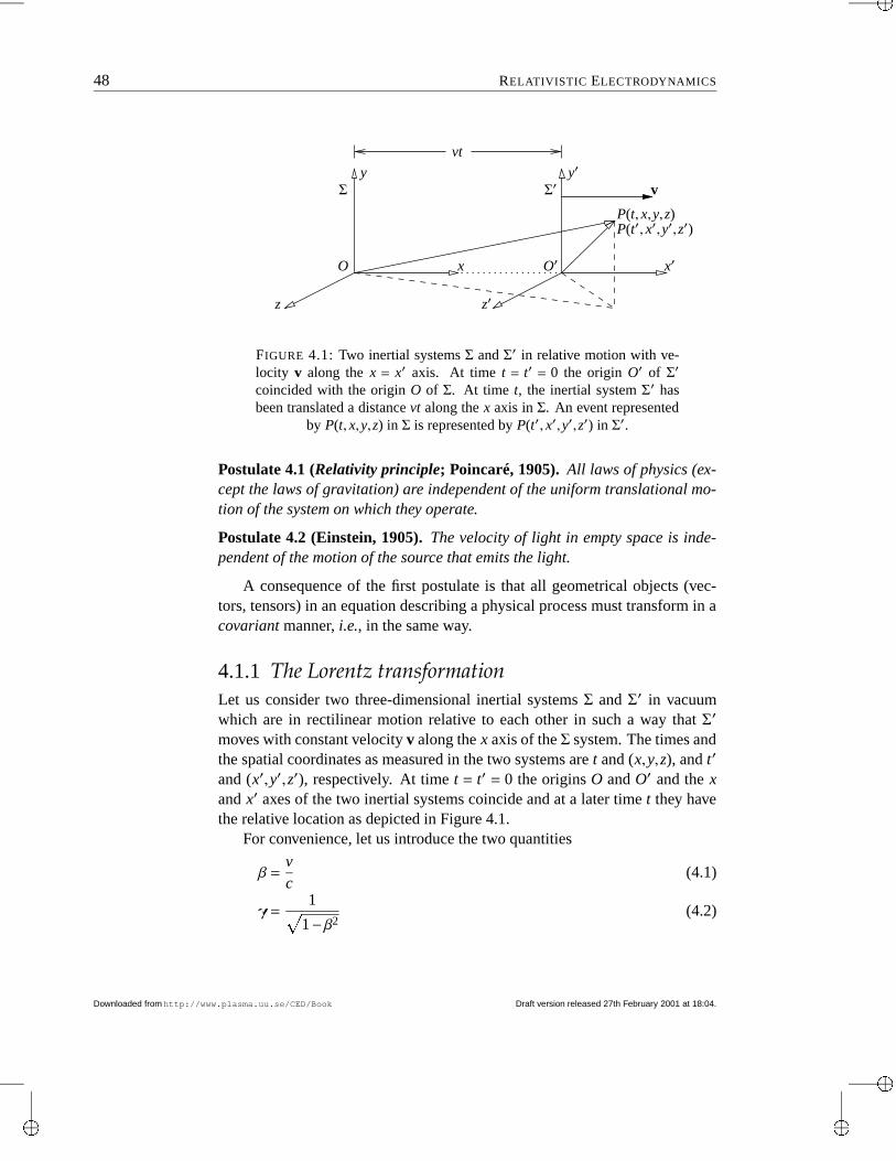
“main”2001/2/27page 48

48 RELATIVISTIC ELECTRODYNAMICS

v

P(t′, x′,y′,z′)

vt

P(t, x,y,z)

z′

x x′

z

O O′

Σ Σ′y y′

FIGURE 4.1: Two inertial systems Σ and Σ′ in relative motion with ve-locity v along the x = x′ axis. At time t = t′ = 0 the origin O′ of Σ′coincided with the origin O of Σ. At time t, the inertial system Σ′ hasbeen translated a distance vt along the x axis in Σ. An event represented

by P(t, x,y,z) in Σ is represented by P(t′, x′,y′,z′) in Σ′.

Postulate 4.1 (Relativity principle; Poincaré, 1905). All laws of physics (ex-cept the laws of gravitation) are independent of the uniform translational mo-tion of the system on which they operate.

Postulate 4.2 (Einstein, 1905). The velocity of light in empty space is inde-pendent of the motion of the source that emits the light.

A consequence of the first postulate is that all geometrical objects (vec-tors, tensors) in an equation describing a physical process must transform in acovariant manner, i.e., in the same way.

4.1.1 The Lorentz transformationLet us consider two three-dimensional inertial systems Σ and Σ′ in vacuumwhich are in rectilinear motion relative to each other in such a way that Σ′

moves with constant velocity v along the x axis of the Σ system. The times andthe spatial coordinates as measured in the two systems are t and (x,y,z), and t′

and (x′,y′,z′), respectively. At time t = t′ = 0 the origins O and O′ and the xand x′ axes of the two inertial systems coincide and at a later time t they havethe relative location as depicted in Figure 4.1.

For convenience, let us introduce the two quantities

β =vc

(4.1)

γ =1;

1−β2(4.2)


“main”2001/2/27page 49

4.1 THE SPECIAL THEORY OF RELATIVITY 49

where v = |v|. In the following, we shall make frequent use of these shorthandnotations.

As shown by Einstein, the two postulates of special relativity require thatthe spatial coordinates and times as measured by an observer in Σ and Σ′,respectively, are connected by the following transformation:

ct′ = γ(ct− xβ) (4.3a)

x′ = γ(x− vt) (4.3b)

y′ = y (4.3c)

z′ = z (4.3d)

Taking the difference between the square of (4.3a) and the square of (4.3b) wefind that

c2t′2− x′2 = γ2 4 c2t2−2xcβt + x2β2− x2 + 2xvt− v2t2 5=

1

1− v2

c2

c2t2 1− v2

c2 − x2 1− v2

c2 = c2t2− x2

(4.4)

From Equations (4.3) above we see that the y and z coordinates are unaffectedby the translational motion of the inertial system Σ′ along the x axis of systemΣ. Using this fact, we find that we can generalise the result in Equation (4.4)to

c2t2− x2− y2− z2 = c2t′2− x′2− y′2− z′2 (4.5)

which means that if a light wave is transmitted from the coinciding originsO and O′ at time t = t′ = 0 it will arrive at an observer at (x,y,z) at time tin Σ and an observer at (x′,y′,z′) at time t′ in Σ′ in such a way that both ob-servers conclude that the speed (spatial distance divided by time) of light invacuum is c. Hence, the speed of light in Σ and Σ′ is the same. A linear coordi-nate transformation which has this property is called a (homogeneous) Lorentztransformation.

4.1.2 Lorentz spaceLet us introduce an ordered quadruple of real numbers, enumerated with thehelp of upper indices µ = 0,1,2,3, where the zeroth component is ct (c is the


“main”2001/2/27page 50


speed of light and t is time), and the remaining components are the componentsof the ordinary 3 radius vector x defined in Equation (M.1) on page 166:

xµ = (x0, x1, x2, x3) = (ct, x,y,z) ≡ (ct,x) (4.6)

We want to interpret this quadruple xµ as (the component form of) a radiusfour-vector in a real, linear, four-dimensional vector space.1 We require thatthis four-dimensional space to be a Riemannian space, i.e., a space where a“distance” and a scalar product are defined. In this space we therefore define ametric tensor, also known as the fundamental tensor, which we denote by gµν.

Radius four-vector in contravariant and covariant form

The radius four-vector xµ = (x0, x1, x2, x3) = (ct,x), as defined in Equation (4.6),is, by definition, the prototype of a contravariant vector (or, more accurately,a vector in contravariant component form). To every such vector there exists adual vector. The vector dual to xµ is the covariant vector xµ, obtained as (theupper index µ in xµ is summed over and is therefore a dummy index and maybe replaced by another dummy index ν):

xµ = gµνxν (4.7)

This summation process is an example of index contraction and is often re-ferred to as index lowering.

Scalar product and norm

The scalar product of xµ with itself in a Riemann space is defined as

gµνxνxµ = xµxµ (4.8)

This scalar product acts as an invariant “distance,” or norm, in this space.If we want the Lorentz transformation invariance, described by Equa-

tion (4.5) on the previous page, to be the manifestation of the conservation

1The British mathematician and philosopher Alfred North Whitehead writes in his book TheConcept of Nature [13]:

“I regret that it has been necessary for me in this lecture to administer a largedose of four-dimensional geometry. I do not apologise, because I am reallynot responsible for the fact that nature in its most fundamental aspect is four-dimensional. Things are what they are. . . ”


“main”2001/2/27page 51


of the norm in a 4D Riemann space, then the explicit expression for the scalarproduct of xµ with itself in this space must be

xµxµ = c2t2− x2− y2− z2 (4.9)

We notice that our space will have an indefinite norm which means that we dealwith a non-Euclidean space. We call the four-dimensional space (or space-time) with this property Lorentz space and denote it < 4 . A corresponding real,linear 4D space with a positive definite norm which is conserved during ordi-nary rotations is a Euclidean vector space. We denote such a space 4 .

Metric tensorBy choosing the metric tensor in < 4 as

gµν = =>? >@ 1 if µ = ν = 0

−1 if µ = ν = i = j = 1,2,3

0 if µ 6= ν

(4.10)

or, in matrix notation,

(gµν) = ABBC 1 0 0 00 −1 0 00 0 −1 00 0 0 −1

DFEEG (4.11)

i.e., a matrix with a main diagonal that has the sign sequence, or signature,+,−,−,−, the index lowering operation in our chosen flat 4D space becomesnearly trivial:

xµ = gµνxν = (ct,−x) (4.12)

Using matrix algebra, this can be written

ABBC x0

x1

x2

x3

DFEEG = ABBC 1 0 0 00 −1 0 00 0 −1 00 0 0 −1

DFEEG ABBC x0

x1

x2

x3

DFEEG = ABBC x0

−x1

−x2

−x3

DFEEG (4.13)

Hence, if the metric tensor is defined according to expression (4.10) the covari-ant radius four-vector xµ is obtained from the contravariant radius four-vectorxµ simply by changing the sign of the last three components. These compo-nents are referred to as the space components; the zeroth component is referredto as the time component.


“main”2001/2/27page 52


As we see, for this particular choice of metric, the scalar product of xµ withitself becomes

xµxµ = (ct,x) · (ct,−x) = c2t2− x2− y2− z2 (4.14)

which indeed is the desired Lorentz transformation invariance as required byEquation (4.9) on the previous page. Without changing the physics, one canalternatively choose a signature −,+,+,+. The latter has the advantage thatthe transition from 3D to 4D becomes smooth, while it will introduce someannoying minus signs in the theory. In current physics literature, the signature+,−,−,− seems to be the most commonly used one.

The < 4 metric tensor Equation (4.10) on the preceding page has a numberof interesting properties: firstly, we see that this tensor has a trace Tr 4 gµν 5 = −2whereas in 4 , as in any vector space with definite norm, the trace equals thespace dimensionality. Secondly, we find, after trivial algebra, that the fol-lowing relations between the contravariant, covariant and mixed forms of themetric tensor hold:

gµν = gνµ (4.15a)

gµν = gµν (4.15b)

gνκgκµ = gµν = δµν (4.15c)

gνκgκµ = gνµ = δνµ (4.15d)

Here we have introduced the 4D version of the Kronecker delta δµν , a mixedfour-tensor of rank 2 which fulfils

δµν = δνµ = H 1 if µ = ν

0 if µ 6= ν(4.16)

Invariant line element and proper time

The differential distance ds between the two points xµ and xµ + dxµ in < 4 canbe calculated from the Riemannian metric, given by the quadratic differentialform

ds2 = gµνdxνdxµ = dxµdxµ = (dx0)2− (dx1)2− (dx2)2− (dx3)2 (4.17)

where the metric tensor is as in Equation (4.10) on the previous page. As wesee, this form is indefinite as expected for a non-Euclidean space. The square


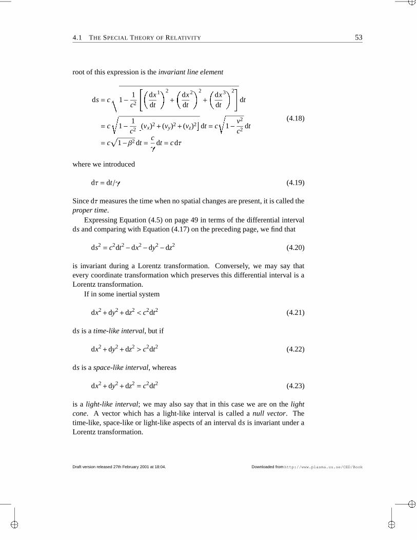
“main”2001/2/27page 53


root of this expression is the invariant line element

ds = c

,--. 1− 1c2 I dx

dt

1 2

+ dxdt

2 2

+ dxdt

3 2 Jdt

= c 1− 1c2 (vx)2 + (vy)2 + (vz)2 dt = c 1− v2

c2 dt

= c;

1−β2 dt =cγ

dt = cdτ

(4.18)

where we introduced

dτ = dt/γ (4.19)

Since dτ measures the time when no spatial changes are present, it is called theproper time.

Expressing Equation (4.5) on page 49 in terms of the differential intervalds and comparing with Equation (4.17) on the preceding page, we find that

ds2 = c2dt2−dx2−dy2−dz2 (4.20)

is invariant during a Lorentz transformation. Conversely, we may say thatevery coordinate transformation which preserves this differential interval is aLorentz transformation.

If in some inertial system

dx2 + dy2 + dz2 < c2dt2 (4.21)

ds is a time-like interval, but if

dx2 + dy2 + dz2 > c2dt2 (4.22)

ds is a space-like interval, whereas

dx2 + dy2 + dz2 = c2dt2 (4.23)

is a light-like interval; we may also say that in this case we are on the lightcone. A vector which has a light-like interval is called a null vector. Thetime-like, space-like or light-like aspects of an interval ds is invariant under aLorentz transformation.


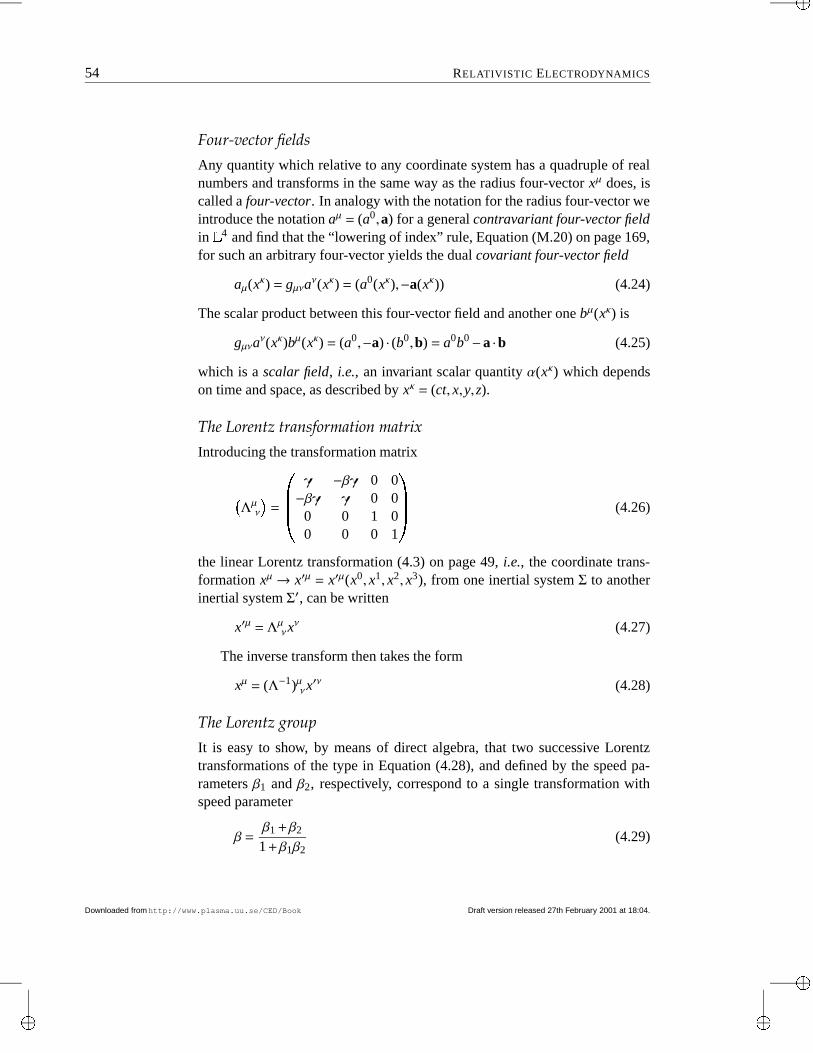
“main”2001/2/27page 54


Four-vector fieldsAny quantity which relative to any coordinate system has a quadruple of realnumbers and transforms in the same way as the radius four-vector xµ does, iscalled a four-vector. In analogy with the notation for the radius four-vector weintroduce the notation aµ = (a0,a) for a general contravariant four-vector fieldin < 4 and find that the “lowering of index” rule, Equation (M.20) on page 169,for such an arbitrary four-vector yields the dual covariant four-vector field

aµ(xκ) = gµνaν(xκ) = (a0(xκ),−a(xκ)) (4.24)

The scalar product between this four-vector field and another one bµ(xκ) is

gµνaν(xκ)bµ(xκ) = (a0,−a) · (b0,b) = a0b0−a ·b (4.25)

which is a scalar field, i.e., an invariant scalar quantity α(xκ) which dependson time and space, as described by xκ = (ct, x,y,z).

The Lorentz transformation matrixIntroducing the transformation matrix

4 Λµν5 = ABBC γ −βγ 0 0

−βγ γ 0 00 0 1 00 0 0 1

DFEEG (4.26)

the linear Lorentz transformation (4.3) on page 49, i.e., the coordinate trans-formation xµ→ x′µ = x′µ(x0, x1, x2, x3), from one inertial system Σ to anotherinertial system Σ′, can be written

x′µ = Λµνxν (4.27)

The inverse transform then takes the form

xµ = (Λ−1)µνx′ν (4.28)

The Lorentz groupIt is easy to show, by means of direct algebra, that two successive Lorentztransformations of the type in Equation (4.28), and defined by the speed pa-rameters β1 and β2, respectively, correspond to a single transformation withspeed parameter

β =β1 +β2

1 +β1β2(4.29)


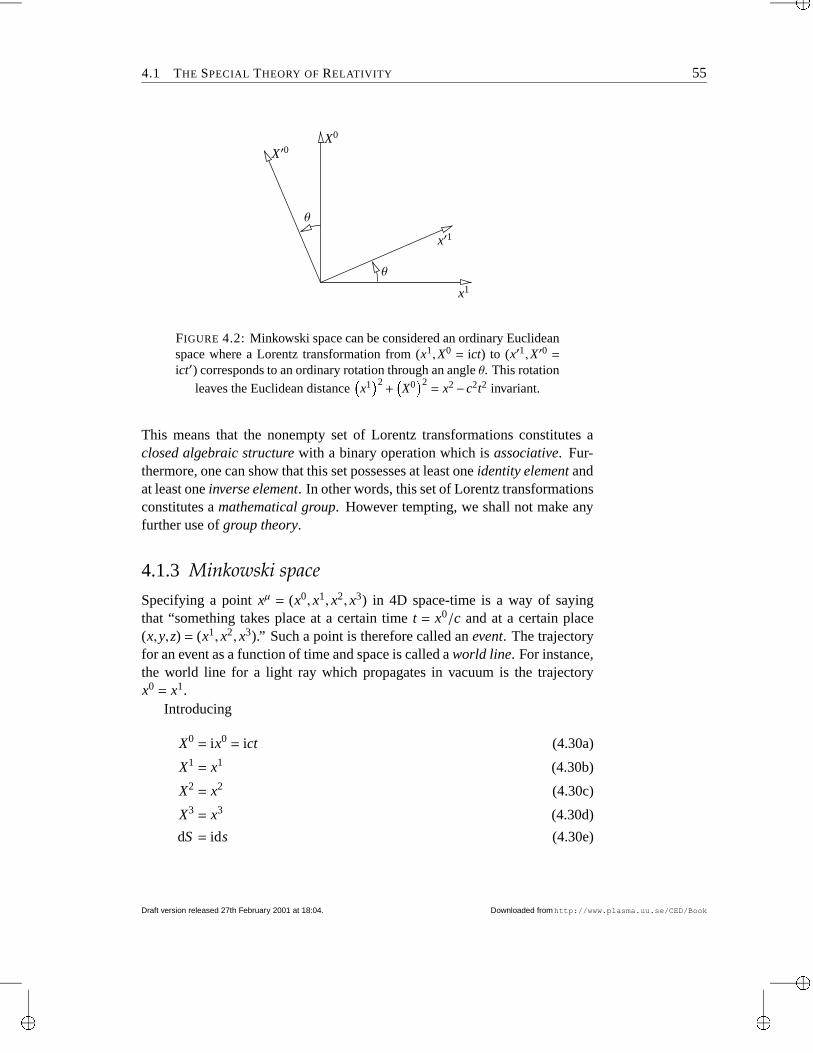
“main”2001/2/27page 55


θ

θ

X′0

x′1

x1

X0

FIGURE 4.2: Minkowski space can be considered an ordinary Euclideanspace where a Lorentz transformation from (x1,X0 = ict) to (x′1,X′0 =

ict′) corresponds to an ordinary rotation through an angle θ. This rotationleaves the Euclidean distance x1 2 + X0 2 = x2 − c2t2 invariant.

This means that the nonempty set of Lorentz transformations constitutes aclosed algebraic structure with a binary operation which is associative. Fur-thermore, one can show that this set possesses at least one identity element andat least one inverse element. In other words, this set of Lorentz transformationsconstitutes a mathematical group. However tempting, we shall not make anyfurther use of group theory.

4.1.3 Minkowski spaceSpecifying a point xµ = (x0, x1, x2, x3) in 4D space-time is a way of sayingthat “something takes place at a certain time t = x0/c and at a certain place(x,y,z) = (x1, x2, x3).” Such a point is therefore called an event. The trajectoryfor an event as a function of time and space is called a world line. For instance,the world line for a light ray which propagates in vacuum is the trajectoryx0 = x1.

Introducing

X0 = ix0 = ict (4.30a)

X1 = x1 (4.30b)

X2 = x2 (4.30c)

X3 = x3 (4.30d)

dS = ids (4.30e)


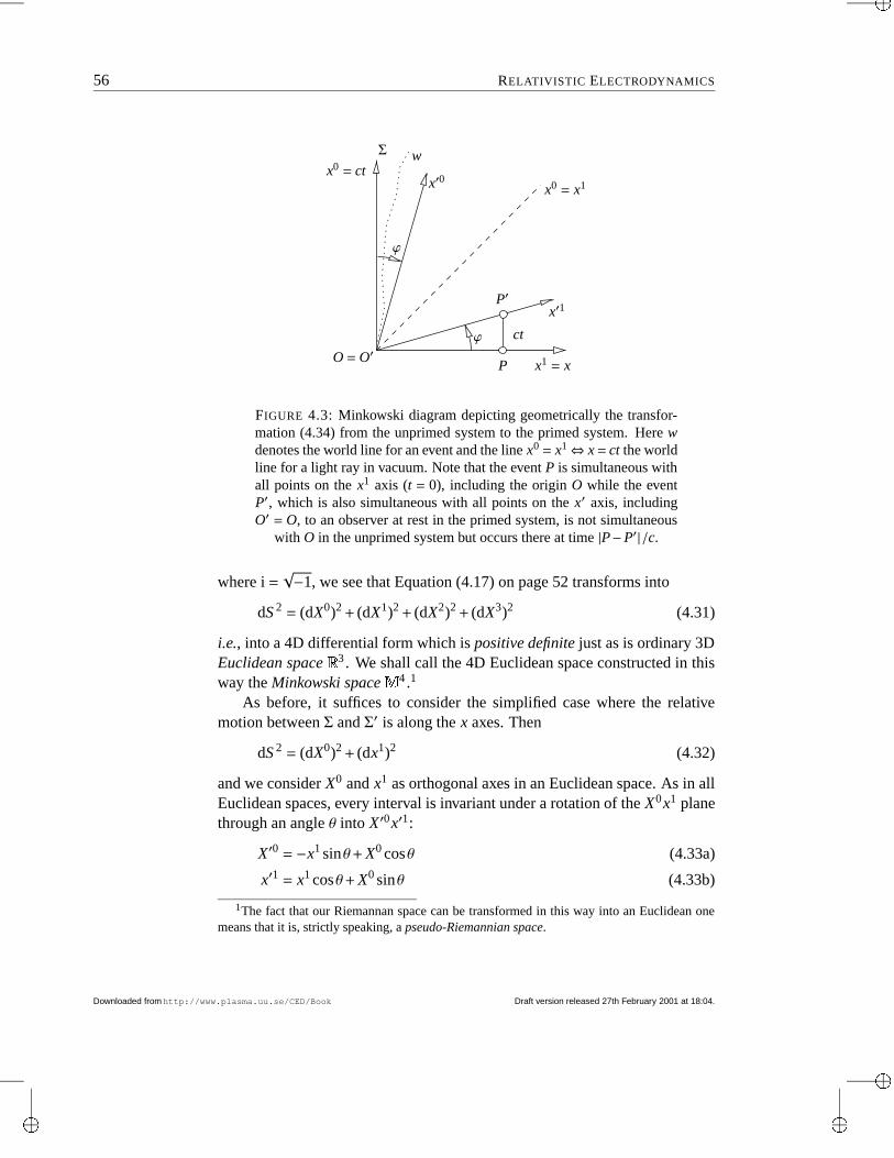
“main”2001/2/27page 56


x0 = ct

ct

x′1

x′0

x1 = xO = O′

ϕ

P

P′

ϕ

x0 = x1

wΣ

FIGURE 4.3: Minkowski diagram depicting geometrically the transfor-mation (4.34) from the unprimed system to the primed system. Here wdenotes the world line for an event and the line x0 = x1⇔ x = ct the worldline for a light ray in vacuum. Note that the event P is simultaneous withall points on the x1 axis (t = 0), including the origin O while the eventP′, which is also simultaneous with all points on the x′ axis, includingO′ = O, to an observer at rest in the primed system, is not simultaneous

with O in the unprimed system but occurs there at time |P−P′|/c.

where i =√−1, we see that Equation (4.17) on page 52 transforms into

dS 2 = (dX0)2 + (dX1)2 + (dX2)2 + (dX3)2 (4.31)

i.e., into a 4D differential form which is positive definite just as is ordinary 3DEuclidean space 3 . We shall call the 4D Euclidean space constructed in thisway the Minkowski space K 4 .1

As before, it suffices to consider the simplified case where the relativemotion between Σ and Σ′ is along the x axes. Then

dS 2 = (dX0)2 + (dx1)2 (4.32)

and we consider X0 and x1 as orthogonal axes in an Euclidean space. As in allEuclidean spaces, every interval is invariant under a rotation of the X0x1 planethrough an angle θ into X′0x′1:

X′0 = −x1 sinθ+ X0 cosθ (4.33a)

x′1 = x1 cosθ+ X0 sinθ (4.33b)

1The fact that our Riemannan space can be transformed in this way into an Euclidean onemeans that it is, strictly speaking, a pseudo-Riemannian space.


“main”2001/2/27page 57

4.2 COVARIANT CLASSICAL MECHANICS 57

See Figure 4.2 on page 55.If we introduce the angle ϕ = −iθ, often called the rapidity or the Lorentz

boost parameter, and transform back to the original space and time variablesby using Equation (4.30) on page 55 backwards, we obtain

ct′ = −xsinhϕ+ ct coshϕ (4.34a)

x′ = xcoshϕ− ct sinhϕ (4.34b)

which are identical to the transformation equations (4.3) on page 49 if we let

sinhϕ = γβ (4.35a)

coshϕ = γ (4.35b)

tanhϕ = β (4.35c)

It is therefore possible to envisage the Lorentz transformation as an “ordinary”rotation in the 4D Euclidean space K 4 This rotation i K 4 corresponds to a co-ordinate change in < 4 as depicted in Figure 4.3 on the preceding page. Equa-tion (4.29) on page 54 for successive Lorentz transformation then correspondsto the tanh addition formula

tanh(ϕ1 +ϕ2) =tanhϕ1 + tanhϕ2

1 + tanhϕ1 tanhϕ2(4.36)

The use of ict and K 4 , which leads to the interpretation of the Lorentztransformation as an “ordinary” rotation, may, at best, be illustrative, but isnot very physical. Besides, if we leave the flat < 4 space and enter the curvedspace of general relativity, the “ict” trick will turn out to be an impasse. Let ustherefore immediately return to < 4 where all components are real valued.

4.2 Covariant Classical MechanicsThe invariance of the differential “distance” ds in < 4 , and the associated dif-ferential proper time dτ [see Equation (4.18) on page 53] allows us to definethe four-velocity

uµ =dxdτ

µ

= γ(c,v) = AC cL1− v2

c2

,vL

1− v2

c2

DG = (u0,u) (4.37)

which, when multiplied with the scalar invariant m0 yields the four-momentum

pµ = m0dxdτ

µ

= m0γ(c,v) = AC m0cL1− v2

c2

,m0vL1− v2

c2

DG = (p0,p) (4.38)


“main”2001/2/27page 58


From this we see that we can write

p = mv (4.39)

where

m = γm0 =m0L1− v2

c2

(4.40)

We can interpret this such that the Lorentz covariance implies that the mass-like term in the ordinary 3D linear momentum is not invariant. A better way tolook at this is that p = mv = γm0v is the covariantly correct expression for thekinetic three-momentum.

Multiplying the zeroth (time) component of the four-momentum pµ withthe scalar invariant c, we obtain

cp0 = γm0c2 =m0c2L1− v2

c2

= mc2 (4.41)

Since this component has the dimension of energy and is the result of a covari-ant description of the motion of a particle with its kinetic momentum describedby the spatial components of the four-momentum, Equation (4.38) on the pre-ceding page, we interpret cp0 as the total energy E. Hence,

cpµ = (cp0,cp) = (E,cp) (4.42)

Scalar multiplying this four-vector with itself, we obtain

cpµcpµ = c2gµνpνpµ = c2[(p0)2− (p1)2− (p2)2− (p3)2]

= (E,−cp) · (E,cp) = E2− c2p2

=(m0c2)2

1− v2

c2

1− v2

c2 = (m0c2)2

(4.43)

Since this is an invariant, this equation holds in any inertial frame, particularlyin the frame where p = 0 and there we have

E = m0c2 (4.44)

This is probably the most famous formula in physics history.


“main”2001/2/27page 59

4.3 COVARIANT CLASSICAL ELECTRODYNAMICS 59

4.3 Covariant Classical ElectrodynamicsIn the rest inertial system the charge density is ρ0. The four-vector (in con-travariant component form)

jµ = ρ0dxµ

dτ= ρ0uµ = ρ0γ(c,v) = (ρc,ρv) (4.45)

where we introduced

ρ = γρ0 (4.46)

is called the four-current.The contravariant form of the four-del operator ∂µ = ∂/∂xµ is defined in

Equation (M.57) on page 177 and its covariant counterpart ∂µ = ∂/∂xµ inEquation (M.58) on page 177, respectively. As is shown in Example M.5 onpage 177, the d’Alembert operator is the scalar product of the four-del withitself: 6 2 = ∂µ∂µ = ∂µ∂

µ =1c2

∂2

∂t2 −∇2 (4.47)

Since it has the characteristics of a four-scalar, the d’Alembert operator is in-variant and, hence, the homogeneous wave equation is Lorentz covariant.

4.3.1 The four-potentialIf we introduce the four-potential

Aµ = φc,A (4.48)

where φ is the scalar potential and A the vector potential, defined in Section 3.3on page 36, we can write the inhomogeneous wave equations (Lorentz equa-tions) Equation (3.15) on page 38 in the following compact (and covariant)way: 6 2Aµ = µ0 jµ (4.49)

With the help of the above, we can formulate our electrodynamic equationscovariantly. For instance, the covariant form of the equation of continuity,Equation (1.21) on page 9 is

∂µ jµ = 0 (4.50)


“main”2001/2/27page 60


and the Lorentz gauge condition, Equation (3.14) on page 38, can be written

∂µAµ = 0 (4.51)

The gauge transformations (3.16) on page 39 in covariant form are

Aµ 7→ A′µ = Aµ +∂µΓ(xν) (4.52)

If only one dimension Lorentz contracts (for instance, due to relative mo-tion along the x direction), a 3D spatial volume transforms according to

dV = d3x =1γ

dV0 = dV0

;1−β2 = dV0 1− v2

c2 (4.53)

then from Equation (4.46) on the previous page we see that

ρdV = ρ0dV0 (4.54)

i.e., the charge in a given volume is conserved. We can therefore conclude thatthe elementary charge is a universal constant.

4.3.2 The Liénard-Wiechert potentialsLet us now solve the Lorentz equation (the inhomogeneous wave equation)(3.15) on page 38 in vacuum for the case of a well-localised charge q′ ata source point defined by the radius four-vector x′µ = (x′0 = ct′, x′1, x′2, x′3).The field point (observation point) is denoted by the radius four-vectorxµ = (x0 = ct, x1, x2, x3).

In the rest system we know that the solution is simply4 Aµ 5 0 = φc,A v=0

= q′

4πε0

1c |x−x′|0

,0 (4.55)

where |x−x′|0 is the usual distance from the source point to the field point,evaluated in the rest system (signified by the index “0”).

Let us introduce the relative radius four-vector between the source pointand the field point:

Rµ = xµ− x′µ = (c(t− t′),x−x′) (4.56)

Scalar multiplying this relative four-vector with itself, we obtain

RµRµ = (c(t− t′),x−x′) · (c(t− t′),−(x−x′)) = c2(t− t′)2− x−x′

2 (4.57)


“main”2001/2/27page 61


We know that in vacuum the signal (field) from the charge q′ at x′µ propa-gates to xµ with the speed of light c so that x−x′

= c(t− t′) (4.58)

Inserting this into Equation (4.57) on the preceding page, we see that

RµRµ = 0 (4.59)

or that Equation (4.56) on the facing page can be written

Rµ = ( x−x′

,x−x′) (4.60)

Now we want to find the correspondence to the rest system solution, Equa-tion (4.55) on the preceding page, in an arbitrary inertial system. We note fromEquation (4.37) on page 57 that in the rest system

4 uµ 5 0 = AC cL1− v2

c2

,vL

1− v2

c2

DGv=0

= (c,0) (4.61)

and

(Rµ)0 = ( x−x′

,x−x′)0 = ( x−x′

0 , (x−x′)0) (4.62)

As all scalar products, uµRµ is invariant, which means that we can evaluateit in any inertial system and it will have the same value in all other inertialsystems. If we evaluate it in the rest system the result is:

uµRµ = 4 uµRµ 5 0 = (uµ)0(Rµ)0

= (c,0) · ( x−x′

0 ,−(x−x′)0) = c

x−x′0

(4.63)

We therefore see that the expression

Aµ =q′

4πε0

uµ

cuνRν(4.64)

subject to the condition RµRµ = 0 has the proper transformation properties(proper tensor form) and reduces, in the rest system, to the solution Equa-tion (4.55) on the preceding page. It is therefore the correct solution, valid inany inertial system.

According to Equation (4.37) on page 57 and Equation (4.60) above

uνRν = γ(c,v) · 4 x−x′ ,−(x−x′) 5 = γ 4 c x−x′

−v · (x−x′) 5 (4.65)


“main”2001/2/27page 62


Generalising expression (4.1) on page 48 to vector form:

β = β vdef≡ v

c(4.66)

and introducing

sdef≡ x−x′

− v · (x−x′)c

≡ x−x′

−β · (x−x′) (4.67)

we can write

uνRν = γcs (4.68)

and

uµ

cuνRν= 1

cs,

vc2s (4.69)

from which we see that the solution (4.64) can be written

Aµ(xκ) =q′

4πε0 1

cs,

vc2s = φ

c,A (4.70)

where in the last step the definition of the four-potential, Equation (4.48) onpage 59, was used. Writing the solution in the ordinary 3D-way, we concludethat for a very localised charge volume, moving relative an observer with avelocity v, the scalar and vector potentials are given by the expressions

φ(t,x) =q′

4πε0

1s

=q′

4πε0

1|x−x′| −β · (x−x′)

(4.71a)

A(t,x) =q′

4πε0c2

vs

=q′

4πε0c2

v|x−x′| −β · (x−x′)

(4.71b)

These potentials are called the Liénard-Wiechert potentials.

4.3.3 The electromagnetic field tensorConsider a vectorial (cross) product c between two ordinary vectors a and b:

c = a×b = εi jkaib j xk = (a2b3−a3b2)x1 + (a3b1−a1b3)x2 + (a1b2−a2b1)x3

(4.72)

We notice that the kth component of the vector c can be represented as

ck = aib j−a jbi = ci j = −c ji, i, j 6= k (4.73)


“main”2001/2/27page 63


In other words, the pseudovector c = a×b can be considered as an antisym-metric tensor of rank two.

The same is true for the curl operator∇×. For instance, the Maxwell equa-tion

∇×E = −∂B∂t

(4.74)

can in this tensor notation be written∂E j

∂xi −∂Ei

∂x j = −∂Bi j

∂t(4.75)

We know from Chapter 3 that the fields can be derived from the electro-magnetic potentials in the following way:

B = ∇×A (4.76a)

E = −∇φ− ∂A∂t

(4.76b)

In component form, this can be written

Bi j =∂A j

∂xi −∂Ai

∂x j = ∂iA j−∂ jAi (4.77a)

Ei = − ∂φ∂xi −

∂Ai

∂t= −∂iφ−∂tAi (4.77b)

From this, we notice the clear difference between the axial vector (pseudovec-tor) B and the polar vector (“ordinary vector”) E.

Our goal is to express the electric and magnetic fields in a tensor formwhere the components are functions of the covariant form of the four-potential,Equation (4.48) on page 59:

Aµ = φc,A (4.78)

Inspection of (4.78) and Equation (4.77) above makes it natural to define thefour-tensor

Fµν =∂Aν

∂xµ− ∂Aµ

∂xν= ∂µAν−∂νAµ (4.79)

This anti-symmetric (skew-symmetric), four-tensor of rank 2 is called the elec-tromagnetic field tensor. In matrix representation, the contravariant field ten-sor can be written

4 Fµν 5 = ABBC 0 −Ex/c −Ey/c −Ez/cEx/c 0 −Bz By

Ey/c Bz 0 −Bx

Ez/c −By Bx 0

DFEEG (4.80)


“main”2001/2/27page 64


The covariant field tensor is obtained from the contravariant field tensor in theusual manner by index contraction (index lowering):

Fµν = gµκgνλFκλ = ∂µAν−∂νAµ (4.81)

It is perhaps interesting to note that the field tensor is a sort of four-dimensionalcurl of the four-potential vector Aµ. The matrix representation for the covariantfield tensor is

4 Fµν5 = ABBC 0 Ex/c Ey/c Ez/c

−Ex/c 0 −Bz By

−Ey/c Bz 0 −Bx

−Ez/c −By Bx 0

DFEEG (4.82)

That the two Maxwell source equations can be written

∂νFνµ = µ0 jµ (4.83)

is immediately observed by explicitly setting µ = 0 in this covariant equationand using the matrix representation Formula (4.80) on the preceding page forthe covariant component form of the electromagnetic field tensor Fµν, to obtain

∂F00

∂x0 +∂F10

∂x1 +∂F20

∂x2 +∂F30

∂x3 = 0 +1c ∂Ex

∂x+∂Ey

∂y+∂Ez

∂z =

1c∇ ·E = µ0 j0 = µ0cρ

(4.84)

or, equivalently,

∇ ·E = µ0c2ρ =ρ

ε0(4.85)

which is the Maxwell source equation for the electric field, Equation (1.43a)on page 14.

For ν = 1, Equation (4.84) yields

∂F01

∂x0 +∂F11

∂x1 +∂F21

∂x2 +∂F31

∂x3 =− 1c2

∂Ex

∂t+0− ∂Bz

∂y+∂By

∂z= µ0 j1 = µ0ρvx (4.86)

or, using ε0µ0 = 1/c2,

∂By

∂z− ∂Bz

∂y−ε0µ0

∂Ex

∂t= µ0 jx (4.87)


“main”2001/2/27page 65

4.3 BIBLIOGRAPHY 65

and similarly for ν = 2,3. In summary, in three-vector form, we can write theresult as


= µ0j(t,x) (4.88)

which is the Maxwell source equation for the magnetic field, Equation (1.43d)on page 14.

The two Maxwell field equations

∇×E = −∂B∂t

(4.89)

∇ ·B = 0 (4.90)

correspond to (no summation!)

∂κFµν +∂µFνκ +∂νFκµ = 0 (4.91)

Hence, Equation (4.83) on the facing page and Equation (4.91) above consti-tute Maxwell’s equations in four-dimensional formalism.

Bibliography[1] J. AHARONI, The Special Theory of Relativity, second, revised ed., Dover Pub-

lications, Inc., New York, 1985, ISBN 0-486-64870-2.

[2] A. O. BARUT, Electrodynamics and Classical Theory of Fields and Particles,Dover Publications, Inc., New York, NY, 1980, ISBN 0-486-64038-8.

[3] R. BECKER, Electromagnetic Fields and Interactions, Dover Publications, Inc.,New York, NY, 1982, ISBN 0-486-64290-9.

[4] D. BOHM, The Special Theory of Relativity, Routledge, New York, NY, 1996,ISBN 0-415-14809-X.

[5] W. T. GRANDY, Introduction to Electrodynamics and Radiation, AcademicPress, New York and London, 1970, ISBN 0-12-295250-2.


[7] F. E. LOW, Classical Field Theory, John Wiley & Sons, Inc., New York, NY . . . ,1997, ISBN 0-471-59551-9.


“main”2001/2/27page 66


[8] C. MØLLER, The Theory of Relativity, second ed., Oxford University Press,Glasgow . . . , 1972.

[9] H. MUIRHEAD, The Special Theory of Relativity, The Macmillan Press Ltd.,London, Beccles and Colchester, 1973, ISBN 333-12845-1.


[11] J. J. SAKURAI, Advanced Quantum Mechanics, Addison-Wesley PublishingCompany, Inc., Reading, MA . . . , 1967, ISBN 0-201-06710-2.

[12] B. SPAIN, Tensor Calculus, third ed., Oliver and Boyd, Ltd., Edinburgh andLondon, 1965, ISBN 05-001331-9.

[13] A. N. WHITEHEAD, Concept of Nature, Cambridge University Press, Cam-bridge . . . , 1920, ISBN 0-521-09245-0.


“main”2001/2/27page 67

5Electromagnetic

Fields andParticles

In previous chapters, we calculated the electromagnetic fields and potentialsfrom arbitrary, but prescribed distributions of charges and currents. In thischapter we study the general problem of interaction between electric and mag-netic fields and electrically charged particles. The analysis is based on La-grangian and Hamiltonian methods, is fully covariant, and yields results whichare relativistically correct.

5.1 Charged Particles in an ElectromagneticField

We first establish a relativistically correct theory describing the motion ofcharged particles in prescribed electric and magnetic fields. From these equa-tions we may then calculate the charged particle dynamics in the most generalcase.

5.1.1 Covariant equations of motionWe can obtain an equation of motion if we find a Lagrange function in 4D forour problem and then apply a variational principle or if we find a Hamiltonianin 4D and solve the corresponding Hamilton’s equations. We shall do both.

Lagrange formalismCall the 4D Lagrange function L(4) and assume that it fulfils the variationalprinciple

δ τ1

τ0

L(4)(xµ,uµ)dτ = 0 (5.1)

67

“main”2001/2/27page 68

68 ELECTROMAGNETIC FIELDS AND PARTICLES

where dτ is the proper time defined via Equation (4.18) on page 53, and theendpoints are fixed.

We must require that L(4) fulfils the following conditions:

1. The Lagrange function must be invariant. This implies that L(4) must bea scalar.

2. The Lagrange function must yield linear equations of motion. This im-plies that L(4) must not contain higher than the second power of the four-velocity uµ.

According to Formula (M.84) on page 182 the ordinary 3D Lagrangian isthe difference between the kinetic and potential energies. A free particle hasonly kinetic energy. If the particle mass is m0 then in 3D the kinetic energy ism0v2/2. This suggests that in 4D the Lagrangian for a free particle should be

Lfree(4) =

12

m0uµuµ (5.2)

For an interaction with the electromagnetic field we can introduce the interac-tion with the help of the four-potential given by Equation (4.78) on page 63 inthe following way

L(4) =12

m0uµuµ + quµAµ(xν) (5.3)

We call this the four-Lagrangian.The variation principle (5.1) with the 4D Lagrangian (5.3) inserted, leads

to

δ τ1

τ0

L(4)(xµ,uµ)dτ = δ τ1

τ0

/ m0

2uµuµ + quµAµ 0 dτ

= τ1

τ0

m0

2∂(uµuµ)∂uµ

δuµ + q Aµδuµ+ uµ∂Aµ∂xν

δxν dτ

= τ1

τ0 m0uµδuµ+ q 4 Aµδuµ + uµ∂νAµδxν 5 dτ = 0

(5.4)

According to Equation (4.37) on page 57, the four-velocity is

uµ =dxdτ

µ

(5.5)

which means that we can write the variation of uµ as a total derivative withrespect to τ :

δuµ = δ dxdτ

µ =ddτ 4 δxµ 5 (5.6)


“main”2001/2/27page 69

5.1 CHARGED PARTICLES IN AN ELECTROMAGNETIC FIELD 69

Inserting this into the first two terms in the last integral in Equation (5.4) onthe facing page, we obtain

δ τ1

τ0

L(4)(xµ,uµ)dτ

= τ1

τ0

m0uµddτ 4 δxµ 5 + qAµ

ddτ 4 δxµ 5 + quµ∂νAµδxν dτ

(5.7)

Partial integration in the two first terms in the right hand member of (5.7)gives

δ τ1

τ0

L(4)(xµ,uµ)dτ

= τ1

τ0

−m0duµdτ

δxµ−qdAµdτ

δxµ+ quµ∂νAµδxν dτ(5.8)

where the integrated parts do not contribute since the variations at the end-points vanish. A change of irrelevant summation index from µ to ν in the firsttwo terms of the right hand member of (5.8) yields, after moving the ensuingcommon factor δxν outside the partenthesis, the following expression:

δ τ1

τ0

L(4)(xµ,uµ)dτ

= τ1

τ0

−m0duνdτ−q

dAνdτ

+ quµ∂νAµ δxνdτ(5.9)

Applying well-known rules of differentiation and the expression (4.37) forthe four-velocity, we can express dAν/dτ as follows:

dAνdτ

=∂Aν∂xµ

dxµ

dτ= ∂µAνu

µ (5.10)

By inserting this expression (5.10) into the second term in right-hand memberof Equation (5.9) above, and noting the common factor quµ of the resultingterm and the last term, we obtain the final variational principle expression

δ τ1

τ0

L(4)(xµ,uµ)dτ

= τ1

τ0

−m0duνdτ

+ quµ 4 ∂νAµ−∂µAν5 δxν dτ

(5.11)

Since, according to the variational principle, this expression shall vanish andδxν is arbitrary between the fixed end points τ0 and τ1, the expression inside Draft version released 27th February 2001 at 18:04. Downloaded fromhttp://www.plasma.uu.se/CED/Book

“main”2001/2/27page 70


in the integrand in the right hand member of Equation (5.11) on the precedingpage must vanish. In other words, we have found an equation of motion for acharged particle in a prescribed electromagnetic field:

m0duνdτ

= quµ 4 ∂νAµ−∂µAν5 (5.12)

With the help of Equation (4.79) on page 63 we can express this equation interms of the electromagnetic field tensor in the following way:

m0duνdτ

= quµFνµ (5.13)

This is the sought-for covariant equation of motion for a particle in an electro-magnetic field. It is often referred to as the Minkowski equation. As the readercan easily verify, the spatial part of this 4-vector equation is the covariant (rel-ativistically correct) expression for the Newton-Lorentz force equation.

Hamiltonian formalism

The usual Hamilton equations for a 3D space are given by Equation (M.89)on page 182 in Appendix M. These six first-order partial differential equationsare

∂H∂pi

=dqi

dt(5.14a)

∂H∂qi

= −dpi

dt(5.14b)

where H(pi,qi, t) = piqi − L(qi, qi, t) is the ordinary 3D Hamiltonian, qi is ageneralised coordinate and pi is its canonically conjugate momentum.

We seek a similar set of equations in 4D space. To this end we introduce acanonically conjugate four-momentum pµ in an analogous way as the ordinary3D conjugate momentum:

pµ =∂L(4)

∂uµ(5.15)

and utilise the four-velocity uµ, as given by Equation (4.37) on page 57, todefine the four-Hamiltonian

H(4) = pµuµ−L(4) (5.16)


“main”2001/2/27page 71


With the help of these, the radius four-vector xµ, considered as the generalisedfour-coordinate, and the invariant line element ds, defined in Equation (4.18)on page 53, we introduce the following eight partial differential equations:

∂H(4)

∂pµ=

dxµdτ

(5.17a)

∂H(4)

∂xµ= −dpµ

dτ(5.17b)

which form the four-dimensional Hamilton equations.Our strategy now is to use Equation (5.15) on the preceding page and Equa-

tions (5.17) to derive an explicit algebraic expression for the canonically con-jugate momentum four-vector. According to Equation (4.42) on page 58, a ctimes a four-momentum has a zeroth (time) component which we can identifywith the total energy. Hence we require that the component p0 of the conju-gate four-momentum vector defined according to Equation (5.15) on the facingpage be identical to the ordinary 3D Hamiltonian H divided by c and hence thatthis cp0 solves the Hamilton equations Equations (5.14) on the preceding page.This later consistency check is left as an exercise to the reader.

Using the definition of H(4), Equation (5.16) on the facing page, and theexpression for L(4), Equation (5.3) on page 68, we obtain

H(4) = pµuµ−L(4) = pµuµ− 12

m0uµuµ−quµAµ(xν) (5.18)

Furthermore, from the definition (5.15) of the canonically conjugate four-momentum pµ, we see that

pµ =∂L(4)

∂uµ=

∂

∂uµ 1

2m0uµuµ + quµAµ(xν) = m0uµ + qAµ (5.19)

Inserting this into (5.18), we obtain

H(4) = m0uµuµ+ qAµuµ− 12

m0uµuµ−quµAµ(xν) =12

m0uµuµ (5.20)

Since the four-velocity scalar-multiplied by itself is uµuµ = c2, we clearlysee from Equation (5.20) that H(4) is indeed a scalar invariant, whose value issimply

H(4) =m0c2

2(5.21)

However, at the same time (5.19) provides the algebraic relationship

uµ =1

m0 4 pµ−qAµ 5 (5.22)


“main”2001/2/27page 72


and if this is used in (5.20) to eliminate uµ, one gets

H(4) =m0

2 1

m0 4 pµ−qAµ 5 1m0 4 pµ−qAµ

5 =

12m0 4 pµ−qAµ 5 4 pµ−qAµ 5

=1

2m0 4 pµpµ−2qAµpµ+ q2AµAµ 5 (5.23)

That this four-Hamiltonian yields the correct covariant equation of motion canbe seen by inserting it into the four-dimensional Hamilton’s equations (5.17)and using the relation (5.22):

∂H(4)

∂xµ= − q

m0(pν−qAν)

∂Aν∂xµ

= − qm0

m0uν∂Aν∂xµ

= −quν∂Aν∂xµ

= −dpµdτ

= −m0duµdτ−q

∂Aµ∂xν

uν

(5.24)

where in the last step Equation (5.19) on the previous page was used. Rear-ranging terms, and using Equation (4.80) on page 63, we obtain

m0duµdτ

= quν 4 ∂µAν−∂νAµ 5 = quνFµν (5.25)

which is identical to the covariant equation of motion Equation (5.13) onpage 70. We can then safely conclude that the Hamiltonian in question iscorrect.

Recalling expression (4.48) on page 59 and representing the canonicallyconjugate four-momentum as pµ = (p0,p), we obtain the following scalar prod-ucts:

pµpµ = (p0)2− (p)2 (5.26a)

Aµpµ =1cφp0− (p ·A) (5.26b)

AµAµ =1c2φ

2− (A)2 (5.26c)

Inserting these explicit expressions into Equation (5.23) above, and using thefact that for H(4) is equal to the scalar value m0c2/2, as derived in Equa-


“main”2001/2/27page 73


tion (5.21) on page 71, we obtain the equation

m0c2

2=

12m0

(p0)2− (p)2− 2c

qφp0 + 2q(p ·A) +q2

c2 φ2−q2(A)2 (5.27)

which is the second order algebraic equation in p0:

(p0)2− 2qcφp0− (p)2−2qp ·A + q2(A)2 M NFO P

(p−qA)2

+q2

c2 φ2−m2

0c2 = 0 (5.28)

with two possible solutions

p0 =qcφ±

L(p−qA)2 + m2

0c2 (5.29)

Since the fourth component (time component) p0 of a four-momentum vectorpµ multiplied by c represents the energy [cf. Equation (4.42) on page 58],the positive solution in Equation (5.29) must be identified with the ordinaryHamilton function H divided by c. Consequently,

H ≡ cp0 = qφ+ cL

(p−qA)2 + m20c2 (5.30)

is the ordinary 3D Hamilton function for a charged particle moving in scalarand vector potentials associated with prescribed electric and magnetic fields.

The ordinary Lagrange and Hamilton functions L and H are related to eachother by the 3D transformation [cf. the 4D transformation (5.16) between L(4)

and H(4)]

L = p ·v−H (5.31)

Using the explicit expressions (Equation (5.30) above) and (Equation (5.31)),we obtain the explicit expression for the ordinary 3D Lagrange function

L = p ·v−qφ− cL

(p−qA)2 + m20c2 (5.32)

and if we make the identification

p−qA =m0vL1− v2

c2

= mv (5.33)

where the quantity mv is the usual kinetic momentum, we can rewrite this ex-pression for the ordinary Lagrangian as follows:

L = qA ·v + mv2 −qφ− cL

m2v2 + m20c2

= mv2−q(φ−A ·v)−mc2 = −qφ+ qA ·v−m0c2 1− v2

c2

(5.34)


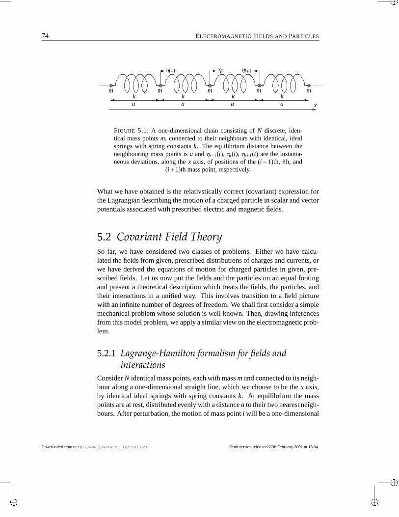
“main”2001/2/27page 74


a

ηi−1 ηi ηi+1

k k kkm m m m

x

m

a a a

FIGURE 5.1: A one-dimensional chain consisting of N discrete, iden-tical mass points m, connected to their neighbours with identical, idealsprings with spring constants k. The equilibrium distance between theneighbouring mass points is a and ηi−1(t), ηi(t), ηi+1(t) are the instanta-neous deviations, along the x axis, of positions of the (i− 1)th, ith, and

(i + 1)th mass point, respectively.

What we have obtained is the relativstically correct (covariant) expression forthe Lagrangian describing the motion of a charged particle in scalar and vectorpotentials associated with prescribed electric and magnetic fields.

5.2 Covariant Field TheorySo far, we have considered two classes of problems. Either we have calcu-lated the fields from given, prescribed distributions of charges and currents, orwe have derived the equations of motion for charged particles in given, pre-scribed fields. Let us now put the fields and the particles on an equal footingand present a theoretical description which treats the fields, the particles, andtheir interactions in a unified way. This involves transition to a field picturewith an infinite number of degrees of freedom. We shall first consider a simplemechanical problem whose solution is well known. Then, drawing inferencesfrom this model problem, we apply a similar view on the electromagnetic prob-lem.

5.2.1 Lagrange-Hamilton formalism for fields andinteractions

Consider N identical mass points, each with mass m and connected to its neigh-bour along a one-dimensional straight line, which we choose to be the x axis,by identical ideal springs with spring constants k. At equilibrium the masspoints are at rest, distributed evenly with a distance a to their two nearest neigh-bours. After perturbation, the motion of mass point i will be a one-dimensional


“main”2001/2/27page 75

5.2 COVARIANT FIELD THEORY 75

oscillatory motion along x. Let us denote the deviation for mass point i fromits equilibrium position by ηi(t)x.

The solution to this mechanical problem can be obtained if we can find aLagrangian (Lagrange function) L which satisfies the variational equation

δ L(ηi, ηi, t)dt = 0 (5.35)

According to Equation (M.84) on page 182, the Lagrangian is L = T −V whereT denotes the kinetic energy and V the potential energy of a classical mechan-ical system with conservative forces. In our case the Lagrangian is

L =12

N

∑i=1 mη2

i − k(ηi+1−ηi)2 (5.36)

Let us write the Lagrangian, as given by Equation (5.36) above, in thefollowing way:

L =N

∑i=1

a Q i (5.37)

Here, Q i =12 m

aη2

i − ka / ηi+1−ηi

a 0 2 (5.38)

is the so called linear Lagrange density. If we now let N→∞ and, at the sametime, let the springs become infinitesimally short according to the followingscheme:

a→ dx (5.39a)

ma→ dm

dx= µ linear mass density (5.39b)

ka→ Y Young’s modulus (5.39c)

ηi+1 −ηi

a→ ∂η

∂x(5.39d)

we obtain

L = Q dx (5.40)

where QR η, ∂η∂t,∂η

∂x, t =

12 I µ ∂η∂t 2

−Y ∂η∂x 2 J

(5.41)


“main”2001/2/27page 76


Notice how we made a transition from a discrete description, in which the masspoints were identified by a discrete integer variable i = 1,2, . . . ,N, to a continu-ous description, where the infinitesimal mass points were instead identified bya continuous real parameter x, namely their position along x.

A consequence of this transition is that the number of degrees of freedomfor the system went from the finite number N to infinity! Another consequenceis that Q has now become dependent also on the partial derivative with respectto x of the “field coordinate” η. But, as we shall see, the transition is wellworth the price because it allows us to treat all fields, be it classical scalaror vectorial fields, or wave functions, spinors and other fields that appear inquantum physics, on an equal footing.

Under the assumption of time independence and fixed endpoints, the vari-ation principle (5.35) on the preceding page yields:

δ Ldt

= δ S Q η, ∂η∂t,∂η

∂x dxdt

= SUTV ∂ Q∂η δη+∂ Q∂ / ∂η∂t 0 δ ∂η∂t +

∂ Q∂ / ∂η∂x 0 δ ∂η∂x WX dxdt

= 0

(5.42)

The last integral can be integrated by parts. This results in the expression

S TV ∂ Q∂η − ∂

∂t AC ∂ Q∂ / ∂η∂t 0 DG − ∂

∂x AC ∂ Q∂ / ∂η∂x 0 DG WX δηdxdt = 0 (5.43)

where the variation is arbitrary (and the endpoints fixed). This means that theintegrand itself must vanish. If we introduce the functional derivative

δ Qδη

=∂ Q∂η− ∂

∂x AC ∂ Q∂ / ∂η∂x 0 DG (5.44)

we can express this as

δ Qδη− ∂

∂t AC ∂ Q∂ / ∂η∂t 0 DG = 0 (5.45)


“main”2001/2/27page 77


which is the one-dimensional Euler-Lagrange equation.Inserting the linear mass point chain Lagrangian density, Equation (5.41)

on page 75, into Equation (5.45) on the facing page, we obtain the equation ofmotion for our one-dimensional linear mechanical structure. It is:

µ∂2

∂t2 η−Y∂2

∂x2 η = µY∂2

∂t2 −∂2

∂x2 η = 0 (5.46)

i.e., the one-dimensional wave equation for compression waves which propa-gate with phase speed vφ =

√Y/µ along the linear structure.

A generalisation of the above 1D results to a three-dimensional continuumis straightforward. For this 3D case we get the variational principle

δ Ldt = δ Q d3xdt

= δ Y QZ η, ∂η∂xµ d4x

= S TV ∂ Q∂η − ∂

∂xµ AC ∂ Q∂ / ∂η∂xµ 0 DG WX δηd4x

= 0

(5.47)

where the variation δη is arbitrary and the endpoints are fixed. This means thatthe integrand itself must vanish:

∂ Q∂η− ∂

∂xµ AC ∂ Q∂ / ∂η∂xµ 0 DG = 0 (5.48)

This constitutes the three-dimensional Euler-Lagrange equations.Introducing the three-dimensional functional derivative

δ Qδη

=∂ Q∂η− ∂

∂xi AC ∂ Q∂ / ∂η

∂xi 0 DG (5.49)

we can express this as

δ Qδη− ∂

∂t AC ∂ Q∂ / ∂η∂t 0 DG = 0 (5.50)


“main”2001/2/27page 78


In analogy with particle mechanics (finite number of degrees of freedom),we may introduce the canonically conjugate momentum density

π(xµ) = π(t,x) =∂ Q∂ / ∂η∂t 0 (5.51)

and define the Hamilton density[ π,η, ∂η∂xi ; t = π

∂η

∂t− QR η, ∂η

∂t,∂η

∂xi (5.52)

If, as usual, we differentiate this expression and identify terms, we obtain thefollowing Hamilton density equations

∂[∂π

=∂η

∂t(5.53a)

δ[δη

= −∂π∂t

(5.53b)

The Hamilton density functions are in many ways similar to the ordinaryHamilton functions and lead to similar results.

The electromagnetic field

Above, when we described the mechanical field, we used a scalar field η(t,x).If we want to describe the electromagnetic field in terms of a Lagrange densityQ and Euler-Lagrange equations, it comes natural to express Q in terms ofthe four-potential Aµ(xκ).

The entire system of particles and fields consists of a mechanical part, afield part and an interaction part. We therefore assume that the total Lagrangedensity Q tot for this system can be expressed asQ tot = Q mech + Q inter + Q field (5.54)

where the mechanical part has to do with the particle motion (kinetic energy).It is given by L(4)/V where L(4) is given by Equation (5.2) on page 68 and V isthe volume. Expressed in the rest mass density %0, the mechanical Lagrangedensity can be writtenQ mech =

12%0uµuµ (5.55)


“main”2001/2/27page 79


The Q inter part which describes the interaction between the charged par-ticles and the external electromagnetic field. A convenient expression for thisinteraction Lagrange density isQ inter = jµAµ (5.56)

For the field part Q field we choose the difference between magnetic andelectric energy density (in analogy with the difference between kinetic andpotential energy in a mechanical field). Using the field tensor, we express thisfield Lagrange density asQ field =

14µ0

FµνFµν (5.57)

so that the total Lagrangian density can be writtenQ tot =12%0uµuµ + jµAµ+

14µ0

FµνFµν (5.58)

From this we can calculate all physical quantities.FIELD ENERGY DIFFERENCE EXPRESSED IN THE FIELD TENSOR EXAMPLE 5.1

Show, by explicit calculation, that

14µ0

FµνFµν =12 B2

µ0−ε0E2 (5.59)

i.e., the difference between the magnetic and electric field energy densities.

From Formula (4.80) on page 63 we recall that

Fµν = !##$ 0 −Ex/c −Ey/c −Ez/cEx/c 0 −Bz By

Ey/c Bz 0 −Bx

Ez/c −By Bx 0' ))+ (5.60)

and from Formula (4.82) on page 64 that Fµν = !##$ 0 Ex/c Ey/c Ez/c−Ex/c 0 −Bz cBy

−Ey/c Bz 0 −cBx

−Ez/c −By Bx 0' ))+ (5.61)

where µ denotes the row number and ν the column number. Then, Einstein summation


“main”2001/2/27page 80


and direct substitution yields

FµνFµν = F00F00 + F01F01 + F02F02 + F03F03

+ F10F10 + F11F11 + F12F12 + F13F13

+ F20F20 + F21F21 + F22F22 + F23F23

+ F30F30 + F31F31 + F32F32 + F33F33

= 0−E2x/c

2 −E2y/c

2 −E2z /c

2

−E2x/c

2 + 0 + B2z + B2

y

−E2y/c

2 + B2z + 0 + B2

x

−E2z /c

2 + B2y + B2

x + 0

= −2E2x −2E2

y/c2 −2E2

z /c2 + B2

x + B2y + B2

z

= −2E2/c2 + 2B2 = 2(B2−E2/c2)

(5.62)

or

14µ0

FµνFµν =12 B2

µ0− 1

c2µ0E2 =

12 B2

µ0−ε0E2 (5.63)

where, in the last step, the identity ε0µ0 = 1/c2 was used. QED END OF EXAMPLE 5.1

Using Q tot in the 3D Euler-Lagrange equations, Equation (5.48) on page 77(with η replaced by Aν), we can derive the dynamics for the whole system. Forinstance, the electromagnetic part of the Lagrangian densityQ EM = Q inter + Q field = jνAν +

14µ0

FµνFµν (5.64)

inserted into the Euler-Lagrange equations, expression (5.48) on page 77, yieldstwo of Maxwell’s equations. To see this, we note from Equation (5.64) and theresults in Example 5.1 that

∂ Q EM

∂Aν= jν (5.65)


“main”2001/2/27page 81


Furthermore,

∂µ ∂ Q EM

∂(∂µAν) =1

4µ0∂µ ∂

∂(∂µAν) 4 FκλFκλ5

=1

4µ0∂µ ∂

∂(∂µAν) (∂κAλ−∂λAκ)(∂κAλ−∂λAκ) =

14µ0

∂µ ∂

∂(∂µAν) ∂κAλ∂κAλ−∂κAλ∂λAκ

−∂λAκ∂κAλ +∂λAκ∂λAκ (=

12µ0

∂µ ∂

∂(∂µAν) 4 ∂κAλ∂κAλ−∂κAλ∂λAκ5

(5.66)

But

∂

∂(∂µAν) 4 ∂κAλ∂κAλ 5 = ∂κAλ∂

∂(∂µAν)∂κAλ +∂κAλ

∂

∂(∂µAν)∂κAλ

= ∂κAλ∂

∂(∂µAν)∂κAλ +∂κAλ

∂

∂(∂µAν)gκα∂αgλβAβ

= ∂κAλ∂

∂(∂µAν)∂κAλ + gκαgλβ∂κAλ

∂

∂(∂µAν)∂αAβ

= ∂κAλ∂

∂(∂µAν)∂κAλ +∂αAβ

∂

∂(∂µAν)∂αAβ

= 2∂µAν

(5.67)

Similarly,

∂

∂(∂µAν) 4 ∂κAλ∂λAκ5 = 2∂νAµ (5.68)

so that

∂µ ∂ Q EM

∂(∂µAν) =1µ0∂µ 4 ∂µAν−∂νAµ 5 =

1µ0∂µFµν (5.69)

This means that the Euler-Lagrange equations, expression (5.48) on page 77,for the Lagrangian density Q EM and with Aν as the field quantity become

∂ Q EM

∂Aν−∂µ ∂ Q EM

∂(∂µAν) = jν− 1µ0∂µFµν = 0 (5.70)


“main”2001/2/27page 82


or

∂µFµν = µ0 jν (5.71)

which, according to Equation (4.83) on page 64, is the covariant version ofMaxwell’s source equations.

Other fields

In general, the dynamic equations for most any fields, and not only electro-magnetic ones, can be derived from a Lagrangian density together with a vari-ational principle (the Euler-Lagrange equations). Both linear and non-linearfields are studied with this technique. As a simple example, consider a real,scalar field η which has the following Lagrange density:Q =

12 4 ∂µη∂µη−m2η2 5 (5.72)

Insertion into the 1D Euler-Lagrange equation, Equation (5.45) on page 76,yields the dynamic equation

(6 2−m2)η = 0 (5.73)

with the solution

η = ei(k·x−ωt) e−m|x|

|x| (5.74)

which describes the Yukawa meson field for a scalar meson with mass m. With

π =1c2

∂η

∂t(5.75)

we obtain the Hamilton density[=

12 c2π2 + (∇η)2 + m2η2 (5.76)

which is positive definite.Another Lagrangian density which has attracted quite some interest is the

Proca LagrangianQ EM = Q inter + Q field = jνAν +1

4µ0FµνFµν + m2AµAµ (5.77)


“main”2001/2/27page 83

5.2 BIBLIOGRAPHY 83

which leads to the dynamic equation

∂µFµν + m2Aν = µ0 jν (5.78)

This equation describes an electromagnetic field with a mass, or, in otherwords, massive photons. If massive photons would exist, large-scale magneticfields, including those of the earth and galactic spiral arms, would be signifi-cantly modified to yield measurable discrepances from their usual form. Spaceexperiments of this kind onboard satellites have led to stringent upper boundson the photon mass. If the photon really has a mass, it will have an impact onelectrodynamics as well as on cosmology and astrophysics.

Bibliography[1] A. O. BARUT, Electrodynamics and Classical Theory of Fields and Particles,

Dover Publications, Inc., New York, NY, 1980, ISBN 0-486-64038-8.

[2] V. L. GINZBURG, Applications of Electrodynamics in Theoretical Physicsand Astrophysics, Revised third ed., Gordon and Breach Science Publishers,New York, London, Paris, Montreux, Tokyo and Melbourne, 1989, ISBN 2-88124-719-9.

[3] H. GOLDSTEIN, Classical Mechanics, second ed., Addison-Wesley PublishingCompany, Inc., Reading, MA . . . , 1981, ISBN 0-201-02918-9.

[4] W. T. GRANDY, Introduction to Electrodynamics and Radiation, AcademicPress, New York and London, 1970, ISBN 0-12-295250-2.



[7] J. J. SAKURAI, Advanced Quantum Mechanics, Addison-Wesley PublishingCompany, Inc., Reading, MA . . . , 1967, ISBN 0-201-06710-2.

[8] D. E. SOPER, Classical Field Theory, John Wiley & Sons, Inc., New York, Lon-don, Sydney and Toronto, 1976, ISBN 0-471-81368-0.


“main”2001/2/27page 84



“main”2001/2/27page 85

6Electromagnetic

Fields andMatter

The microscopic Maxwell equations (1.43) derived in Chapter 1 are valid on allscales where a classical description is good. However, when macroscopic mat-ter is present, it is sometimes convenient to use the corresponding macroscopicMaxwell equations (in a statistical sense) in which auxiliary, derived fields areintroduced in order to incorporate effects of macroscopic matter when this isimmersed fully or partially in an electromagnetic field.

6.1 Electric Polarisation and DisplacementIn certain cases, for instance in engneering applications, it may be convenientto separate the influence of an external electric field on free charges and onneutral matter in bulk. This view, which, as we shall see, has certain lim-itations, leads to the introduction of (di)electric polarisation and (di)electricpolarisation.

6.1.1 Electric multipole momentsThe electrostatic properties of a spatial volume containing electric charges andlocated near a point x0 can be characterized in terms of the total charge orelectric monopole moment

q = Vρ(x′)d3x′ (6.1)

where the ρ is the charge density introduced in Equation (1.7) on page 4, theelectric dipole moment vector

p = V(x′−x0)ρ(x′)d3x′ (6.2)

85

“main”2001/2/27page 86

86 ELECTROMAGNETIC FIELDS AND MATTER

with components pi, i = 1,2,3, the electric quadrupole moment tensor

Q = V(x′−x0)(x′−x0)ρ(x′)d3x′ (6.3)

with components Qi j, i, j = 1,2,3, and higher order electric moments.In particular, the electrostatic potential Equation (3.3) on page 35 from a

charge distribution located near x0 can be Taylor expanded in the followingway:

φstat(x) =1

4πε0 q|x−x0| +

1

|x−x0|2pi

(x−x0)i

|x−x0|

+1

|x−x0|3Qi j 3

2(x−x0)i

|x−x0|(x−x0) j

|x−x0| −12δi j + . . . (6.4)

where Einstein’s summation convention over i and j is implied. As can beseen from this expression, only the first few terms are important if the fieldpoint (observation point) is far away from x0.

For a normal medium, the major contributions to the electrostatic interac-tions come from the net charge and the lowest order electric multipole mo-ments induced by the polarisation due to an applied electric field. Particularlyimportant is the dipole moment. Let P denote the electric dipole moment den-sity (electric dipole moment per unit volume; unit: C/m2), also known as theelectric polarisation, in some medium. In analogy with the second term in theexpansion Equation (6.4) on page 86, the electric potential from this volumedistribution P(x′) of electric dipole moments p at the source point x′ can bewritten

φp(x) =1

4πε0 VP(x′) · x−x′

|x−x′|3 d3x′ = − 14πε0 V

P(x′) ·∇ 1|x−x′| d3x′

=1

4πε0 VP(x′) ·∇′ 1

|x−x′| d3x′

(6.5)

Using the expression Equation (M.71) on page 179 and applying the diver-gence theorem, we can rewrite this expression for the potential as follows:

φp(x) =1

4πε0 V∇′ · P(x′)

|x−x′| d3x′− V

∇′ ·P(x′)|x−x′| d3x′

=1

4πε0 S

P(x′) · n|x−x′| d2x− V

∇′ ·P(x′)|x−x′| d3x′ (6.6)


“main”2001/2/27page 87

6.1 ELECTRIC POLARISATION AND DISPLACEMENT 87

where the first term, which describes the effects of the induced, non-cancellingdipole moment on the surface of the volume, can be neglected, unless there isa discontinuity in P · n at the surface. Doing so, we find that the contributionfrom the electric dipole moments to the potential is given by

φp =1

4πε0 V

−∇′ ·P(x′)|x−x′| d3x′ (6.7)

Comparing this expression with expression Equation (3.3) on page 35 for theelectrostatic potential from a static charge distribution ρ, we see that −∇ ·P(x)has the characteristics of a charge density and that, to the lowest order, theeffective charge density becomes ρ(x)−∇ ·P(x), in which the second term is apolarisation term.

The version of Equation (1.7) on page 4 where “true” and polarisationcharges are separated thus becomes

∇ ·E =ρ(x)−∇ ·P(x)

ε0(6.8)

Rewriting this equation, and at the same time introducing the electric displace-ment vector (C/m2)

D = ε0E + P (6.9)

we obtain

∇ · (ε0E + P) = ∇ ·D = ρtrue(x) (6.10)

where ρtrue is the “true” charge density in the medium. This is one of Maxwell’sequations and is valid also for time varying fields. By introducing the no-tation ρpol = −∇ · P for the “polarised” charge density in the medium, andρtotal = ρtrue + ρpol for the “total” charge density, we can write down the fol-lowing alternative version of Maxwell’s equation (6.23a) on page 90

∇ ·E =ρtotal(x)ε0

(6.11)

Often, for low enough field strengths |E|, the linear and isotropic relation-ship between P and E

P = ε0χE (6.12)

is a good approximation. The quantity χ is the electric susceptibility whichis material dependent. For electromagnetically anisotropic media such as a


“main”2001/2/27page 88


magnetised plasma or a birefringent crystal, the susceptibility is a tensor. Ingeneral, the relationship is not of a simple linear form as in Equation (6.12)on the previous page but non-linear terms are important. In such a situationthe principle of superposition is no longer valid and non-linear effects such asfrequency conversion and mixing can be expected.

Inserting the approximation (6.12) into Equation (6.9) on the precedingpage, we can write the latter

D = εE (6.13)

where, approximately,

ε = ε0(1 +χ) (6.14)

6.2 Magnetisation and the Magnetising FieldAn analysis of the properties of stationary magnetic media and the associatedcurrents shows that three such types of currents exist:

1. In analogy with “true” charges for the electric case, we may have “true”currents jtrue, i.e., a physical transport of true charges.

2. In analogy with electric polarisation P there may be a form of chargetransport associated with the changes of the polarisation with time. Wecall such currents induced by an external field polarisation currents. Weidentify them with ∂P/∂t.

3. There may also be intrinsic currents of a microscopic, often atomic, na-ture that are inaccessible to direct observation, but which may producenet effects at discontinuities and boundaries. We shall call such currentsmagnetisation currents and denote them jM.

No magnetic monopoles have been observed yet. So there is no correspon-dence in the magnetic case to the electric monopole moment (6.1). The lowestorder magnetic moment, corresponding to the electric dipole moment (6.2), isthe magnetic dipole moment

m =12 V

(x′−x0)× j(x′)d3x′ (6.15)

For a distribution of magnetic dipole moments in a volume, we may describethis volume in terms of the magnetisation, or magnetic dipole moment per unit


“main”2001/2/27page 89

6.2 MAGNETISATION AND THE MAGNETISING FIELD 89

volume, M. Via the definition of the vector potential one can show that themagnetisation current and the magnetisation is simply related:

jM = ∇×M (6.16)

In a stationary medium we therefore have a total current which is (approx-imately) the sum of the three currents enumerated above:

jtotal = jtrue +∂P∂t

+∇×M (6.17)

We might then, erroneously, be led to think that

∇×B = µ0 jtrue +∂P∂t

+∇×M (6.18)

Moving the term ∇×M to the left hand side and introducing the magnetisingfield (magnetic field intensity, Ampère-turn density) as

H =Bµ0−M (6.19)

and using the definition for D, Equation (6.9) on page 87, we can write thisincorrect equation in the following form

∇×H = jtrue +∂P∂t

= jtrue +∂D∂t−ε0

∂E∂t

(6.20)

As we see, in this simplistic view, we would pick up a term which makesthe equation inonsistent; the divergence of the left hand side vanishes whilethe divergence of the right hand side does not. Maxwell realised this and toovercome this inconsistency he was forced to add his famous displacementcurrent term which precisely compensates for the last term in the right handside. In Chapter 1, we discussed an alternative way, based on the postulate ofconservation of electric charge, to introduce the displacement current.

We may, in analogy with the electric case, introduce a magnetic suscepti-bility for the medium. Denoting it χm, we can write

H =Bµ

(6.21)

where, approximately,

µ = µ0(1 +χm) (6.22)


“main”2001/2/27page 90


Maxwell’s equations expressed in terms of the derived field quantities Dand H are

∇ ·D = ρ(t,x) (6.23a)

∇ ·B = 0 (6.23b)

∇×E = −∂B∂t

(6.23c)

∇×H = j(t,x) +∂

∂tD (6.23d)

and are called Maxwell’s macroscopic equations. These equations are conve-nient to use in certain simple cases. Together with the boundary conditions andthe constitutive relations, they describe uniquely (but only approximately!) theproperties of the electric and magnetic fields in matter.

6.3 Energy and MomentumWe shall use Maxwells macroscopic equations in the following considerationson the energy and momentum of the electromagnetic field and its interactionwith matter.

6.3.1 The energy theorem in Maxwell’s theoryScalar multiplying (6.23c) by H, (6.23d) by E and subtracting, we obtain

H · (∇×E)−E · (∇×H) = ∇ · (E×H)

= −H · ∂B∂t−E · j−E · ∂D

∂t= −1

2∂

∂t(H ·B + E ·D)− j ·E

(6.24)

Integration over the entire volume V and using Gauss’s theorem (the diver-gence theorem), we obtain

− ∂∂t V

12

(H ·B + E ·D)d3x′ = Vj ·Ed3x′+ S

(E×H) · nd2x′ (6.25)

But, according to Ohm’s law in the presence of an electromotive forcefield, Equation (1.26) on page 10:

j = σ(E + EEMF) (6.26)

which means that Vj ·Ed3x′ = V

j2

σd3x′− V

j ·EEMF d3x′ (6.27)


“main”2001/2/27page 91

6.3 ENERGY AND MOMENTUM 91

Inserting this into Equation (6.25) on the preceding page

Vj ·EEMF d3x′M NFO P

Applied electric power

= V

j2

σd3x′M NFO P

Joule heat

+∂

∂t V

12

(E ·D + H ·B)d3x′M NFO PField energy

+ S(E×H) · nd2x′M N\O PRadiated power

(6.28)

which is the energy theorem in Maxwell’s theory also known as Poynting’stheorem.

It is convenient to introduce the following quantities:

Ue =12 V

E ·Dd3x′ (6.29)

Um =12 V

H ·Bd3x′ (6.30)

S = E×H (6.31)

where Ue is the electric field energy, Um is the magnetic field energy, bothmeasured in J, and S is the Poynting vector (power flux), measured in W/m2.

6.3.2 The momentum theorem in Maxwell’s theoryLet us now investigate the momentum balance (force actions) in the case thata field interacts with matter in a non-relativistic way. For this purpose weconsider the force density given by the Lorentz force per unit volume ρE+j×B.Using Maxwell’s equations (6.23) and symmetrising, we obtain

ρE + j×B = (∇ ·D)E + ∇×H− ∂D∂t ×B

= E(∇ ·D) + (∇×H)×B− ∂D∂t×B

= E(∇ ·D)−B× (∇×H)

− ∂

∂t(D×B) + D× ∂B

∂t= E(∇ ·D)−B× (∇×H)

− ∂

∂t(D×B)−D× (∇×E) + H(∇ ·BM NFO P

=0

)

= [E(∇ ·D)−D× (∇×E)] + [H(∇ ·B)−B× (∇×H)]

− ∂

∂t(D×B)

(6.32)


“main”2001/2/27page 92


One verifies easily that the ith vector components of the two terms insquare brackets in the right hand member of (6.32) can be expressed as

[E(∇ ·D)−D× (∇×E)]i =12 E · ∂D

∂xi−D · ∂E

∂xi +∂

∂x j EiD j− 1

2E ·Dδi j

(6.33)

and

[H(∇ ·B)−B× (∇×H)]i =12 H · ∂B

∂xi−B · ∂H

∂xi +∂

∂x j HiB j− 1

2B ·Hδi j

(6.34)

respectively.Using these two expressions in the ith component of Equation (6.32) on

the preceding page and re-shuffling terms, we get

(ρE + j×B)i− 12] E · ∂D

∂xi−D · ∂E

∂xi + H · ∂B∂xi−B · ∂H

∂xi ^ +∂

∂t(D×B)i

=∂

∂x j EiD j− 1

2E ·Dδi j + HiB j− 1

2H ·Bδi j

(6.35)

Introducing the electric volume force Fev via its ith component

(Fev)i = (ρE+ j×B)i− 12] E · ∂D

∂xi−D · ∂E

∂xi + H · ∂B∂xi−B · ∂H

∂xi 1 (6.36)

and the Maxwell stress tensor T with components

Ti j = EiD j− 12

E ·Dδi j + HiB j− 12

H ·Bδi j (6.37)

we finally obtain the force equation Fev +∂

∂t(D×B) i

=∂Ti j

∂x j= (∇ ·T)i (6.38)

If we introduce the relative electric permittivity κ and the relative magneticpermeability κm as

D = κε0E = εE (6.39)

B = κmµ0H = µH (6.40)


“main”2001/2/27page 93

6.3 BIBLIOGRAPHY 93

we can rewrite (6.38) as

∂Ti j

∂x j= Fev +

κκm

c2

∂S∂t i

(6.41)

where S is the Poynting vector defined in Equation (6.29) on page 91. Integra-tion over the entire volume V yields V

Fev d3x′M NFO PForce on the matter

+ddt V

κκm

c2 Sd3x′M NFO PField momentum

= STn d2x′M NFO P

Maxwell stress

(6.42)

which expresses the balance between the force on the matter, the rate of changeof the electromagnetic field momentum and the Maxwell stress. This equationis called the momentum theorem in Maxwell’s theory.

In vacuum (6.42) becomes Vρ(E + v×B)d3x′+

1c2

ddt V

Sd3x′ = STn d2x′ (6.43)

or

ddt

pmech +ddt

pfield = STn d2x′ (6.44)

Bibliography[1] E. HALLÉN, Electromagnetic Theory, Chapman & Hall, Ltd., London, 1962.





“main”2001/2/27page 94



“main”2001/2/27page 95

7Electromagnetic

Fields fromArbitrary Source

Distributions

While, in principle, the electric and magnetic fields can be calculated from theMaxwell equations in Chapter 1, or even from the wave equations in Chapter 2,it is often physically more lucid to calculate them from the electromagneticpotentials derived in Chapter 3. In this chapter we will derive the electric andmagnetic fields from the potentials.

We recall that in order to find the solution (3.36) for the generic inhomo-geneous wave equation (3.20) on page 40 we presupposed the existence of aFourier transform pair (3.21a) on page 41 for the generic source term

Ψ(t,x) = ∞−∞Ψω(x)e−iωtdω (7.1a)

Ψω(x) =1

2π ∞−∞Ψ(t,x)eiωtdt (7.1b)

That such transform pairs exists is true for most physical variables which arenot strictly monotonically increasing and decreasing with time. For chargesand currents varying in time we can therefore, without loss of generality, workwith individual Fourier components. Strictly speaking, the existence of a singleFourier component assumes a monochromatic source (i.e., a source containingonly one single frequency component), which in turn requires that the electricand magnetic fields exist for infinitely long times. However, by taking theproper limits, we can still use this approach even for sources and fields offinite duration.

This is the method we shall utilise in this chapter in order to derive theelectric and magnetic fields in vacuum from arbitrary given charge densitiesρ(t,x) and current densities j(t,x), defined by the temporal Fourier transform

95

“main”2001/2/27page 96


pairs

ρ(t,x) = ∞−∞ ρω(x)e−iωtdω (7.2a)

ρω(x) =1

2π ∞−∞ ρ(t,x)eiωtdt (7.2b)

and

j(t,x) = ∞−∞ jω(x)e−iωtdω (7.3a)

jω(x) =1

2π ∞−∞ j(t,x)eiωtdt (7.3b)

under the assumption that only retarded potentials produce physically accept-able solutions.1

The temporal Fourier transform pair for the retarded vector potential canthen be written

φ(t,x) = ∞−∞φω(x)e−iωtdω (7.4a)

φω(x) =1

2π ∞−∞φ(t,x)eiωtdt =1

4πε0 ρω(x′)eik|x−x′ |

|x−x′| d3x′ (7.4b)

where in the last step, we made use of the explicit expression for the temporalFourier transform of the generic potential component Ψω(x), Equation (3.33)on page 43. Similarly, the following Fourier transform pair for the vector po-tential must exist:

A(t,x) = ∞−∞Aω(x)e−iωtdω (7.5a)

Aω(x) =1

2π ∞−∞A(t,x)eiωtdt =µ0

4π jω(x′)eik|x−x′ |

|x−x′| d3x′ (7.5b)

Clearly, we must require that

Aω = A∗−ω, φω = φ∗−ω (7.6)

in order that all physical quantities be real. Similar transform pairs and re-quirements of real-valuedness exist for the fields themselves.

1In fact, John A. Wheeler and Richard P. Feynman derived in 1945 a fully self-consistentelectrodynamics using both the retarded and the advanced potentials [6]; See also [1].


“main”2001/2/27page 97

7.1 THE MAGNETIC FIELD 97

In the limit that the sources can be considered monochromatic containingonly one single frequency ω0, we have the much simpler expressions

ρ(t,x) = ρ0(x)e−iω0t (7.7a)

j(t,x) = j0(x)e−iω0t (7.7b)

φ(t,x) = φ0(x)e−iω0t (7.7c)

A(t,x) = A0(x)e−iω0t (7.7d)

where again the real-valuedness of all these quantities is implied. As discussedabove, we can safely assume that all formulae derived for a general temporalFourier representation of the source (general distribution of frequencies in thesource) are valid for these simple limiting cases. We note that in this context,we can make the formal identification ρω = ρ0δ(ω−ω0), jω = j0δ(ω−ω0) etc.,and that we therefore, without any loss of stringence, let ρ0 mean the same asthe Fourier amplitude ρω and so on.

7.1 The Magnetic FieldLet us now compute the magnetic field from the vector potential, defined byEquation (7.5a) and Equation (7.5b) on the preceding page, and Formula (3.7)on page 37:

B(t,x) = ∇×A(t,x) (7.8)

The calculations are much simplified if we work in ω space and, at thefinal stage, Fourier transform back to ordinary t space. We are working in theLorentz gauge and note that in ω space the Lorentz condition, Equation (3.14)on page 38, takes the form

∇ ·Aω − ikcφω = 0 (7.9)

which provides a relation between (the Fourier transforms of) the vector andscalar potentials.

Using the Fourier transformed version of Equation (7.8) and Equation (7.5b)on the preceding page, we obtain

Bω(x) = ∇×Aω(x) =µ0

4π∇× V

jω(x′)eik|x−x′ |

|x−x′| d3x′ (7.10)


“main”2001/2/27page 98

98 ELECTROMAGNETIC FIELDS FROM ARBITRARY SOURCE DISTRIBUTIONS

Using Formula (F.60) on page 163, we can rewrite this as

Bω(x) = −µ0

4π Vjω(x′)× ∇ eik|x−x′ |

|x−x′| d3x′

= −µ0

4π V

jω(x′)× − x−x′

|x−x′|3 eik|x−x′ | d3x′

+ Vjω(x′)× ik

x−x′

|x−x′|eik|x−x′ | 1

|x−x′| d3x′

=µ0

4π V

jω(x′)eik|x−x′ |× (x−x′)|x−x′|3 d3x′

+ V

(−ik)jω(x′)eik|x−x′ |× (x−x′)|x−x′|2 d3x′

(7.11)

From this expression for the magnetic field in the frequency (ω) domain,we obtain the total magnetic field in the temporal (t) domain by taking theinverse Fourier transform (using the identity −ik = −iω/c):

B(t,x) = ∞−∞Bω(x)e−iωtdω

=µ0

4π V

jω(x′)ei(k|x−x′ |−ωt) dω × (x−x′)|x−x′|3 d3x′

+1c V

(−iω)jω(x′)ei(k|x−x′ |−ωt) dω × (x−x′)|x−x′|2 d3x′

=µ0

4π V

j(t′ret,x′)× (x−x′)|x−x′|3 d3x′M N\O P

Induction field

+µ0

4πc V

j(t′ret,x′)× (x−x′)|x−x′|2 d3x′M N\O P

Radiation field

(7.12)

where

j(t′ret,x′)

def≡ ∂j∂t t=t′ret

(7.13)

The first term, the induction field, dominates near the current source but fallsoff rapidly with distance from it, is the electrodynamic version of the Biot-Savart law in electrostatics, Formula (1.13) on page 6. The second term, theradiation field or the far field, dominates at large distances and represents en-ergy that is transported out to infinity. Note how the spatial derivatives (∇)gave rise to a time derivative ( )!


“main”2001/2/27page 99

7.2 THE ELECTRIC FIELD 99

7.2 The Electric FieldIn order to calculate the electric field, we use the temporally Fourier trans-formed version of Formula (3.11) on page 37, inserting Equations (7.4b) and(7.5b) as the explicit expressions for the Fourier transforms of φ and A:

Eω(x) = −∇φω(x) + iωAω(x)

= − 14πε0

∇ Vρω(x′)

eik|x−x′ |

|x−x′| d3x′+

iµ0ω

4π Vjω(x′)

eik|x−x′ |

|x−x′| d3x′

=1

4πε0 V

ρω(x′)eik|x−x′ |(x−x′)|x−x′|3 d3x′

− ik V ρω(x′)(x−x′)

|x−x′| − jω(x′)c eik|x−x′ |

|x−x′| d3x′

(7.14)

Using the Fourier transform of the continuity Equation (1.21) on page 9

∇′ · jω(x′)− iωρω(x′) = 0 (7.15)

we see that we can express ρω in terms of jω as follows

ρω(x′) = − iω∇′ · jω(x′) (7.16)

Doing so in the last term of Equation (7.14), and also using the fact that k =

ω/c, we can rewrite this Equation as

Eω(x) =1

4πε0 V


− 1c V

[∇′ · jω(x′)](x−x′)|x−x′| − ikjω(x′) eik|x−x′ |

|x−x′| d3x′M NFO P

Iω

(7.17)

The last integral can be further rewritten in the following way:

Iω = V [∇′ · jω(x′)](x−x′)

|x−x′| − ikjω(x′) eik|x−x′ |

|x−x′| d3x′

= V ∂ jωm

∂x′m

xl− x′l|x−x′| − ik jωl(x′) xl

eik|x−x′ |

|x−x′| d3x′

(7.18)

But, since

∂

∂x′m jωm

xl− x′l|x−x′|2 eik|x−x′ | = ∂ jωm

∂x′m xl− x′l|x−x′|2 eik|x−x′ |

+ jωm∂

∂x′m xl− x′l|x−x′|2 eik|x−x′ | (7.19)


“main”2001/2/27page 100


we can rewrite Iω as

Iω = − V jωm

∂

∂x′m xl− x′l|x−x′|2 xl eik|x−x′ | + ikjω

eik|x−x′ |

|x−x′| d3x′

+ V

∂

∂x′m jωm

xl− x′l|x−x′|2 xl e

ik|x−x′ | d3x′(7.20)

where, according to Gauss’s theorem, the last term vanishes if jω is assumedto be limited and tends to zero at large distances. Further evaluation of thederivative in the first term makes it possible to write

Iω = − V −jω

eik|x−x′ |

|x−x′|2 +2

|x−x′|4 jω · (x−x′) (x−x′)eik|x−x′ | d3x′

− ik V _ − jω · (x−x′) (x−x′)|x−x′|3 eik|x−x′ |+ jω

eik|x−x′ |

|x−x′| ` d3x′(7.21)

Using the triple product “bac-cab” Formula (F.54) on page 162 backwards, andinserting the resulting expression for Iω into Equation (7.17) on the precedingpage, we arrive at the following final expression for the Fourier transform ofthe total E-field:

Eω(x) = − 14πε0

∇ Vρω(x′)

eik|x−x′ |

|x−x′| d3x′+

iµ0ω

4π Vjω(x′)

eik|x−x′ |

|x−x′| d3x′

=1

4πε0 V


+1c V

[jω(x′)eik|x−x′ | · (x−x′)](x−x′)|x−x′|4 d3x′

+1c V

[jω(x′)eik|x−x′ |× (x−x′)]× (x−x′)|x−x′|4 d3x′

− ikc V

[jω(x′)eik|x−x′ |× (x−x′)]× (x−x′)|x−x′|3 d3x′

(7.22)

Taking the inverse Fourier transform of Equation (7.22) above, once againusing the vacuum relation ω = kc, we find, at last, the expression in time do-


“main”2001/2/27page 101

7.3 THE RADIATION FIELDS 101

main for the total electric field:

E(t,x) = ∞−∞Eω(x)e−iωtdω

=1

4πε0 V

ρ(t′ret,x′)(x−x′)

|x−x′|3 d3x′M NFO PRetarded Coulomb field

+1

4πε0c V

[j(t′ret,x′) · (x−x′)](x−x′)|x−x′|4 d3x′M N\O P

Intermediate field

+1

4πε0c V

[j(t′ret,x′)× (x−x′)]× (x−x′)|x−x′|4 d3x′M NFO P

Intermediate field

+1

4πε0c2 V

[j(t′ret,x′)× (x−x′)]× (x−x′)|x−x′|3 d3x′M N\O P

Radiation field

(7.23)

Here, the first term represents the retarded Coulomb field and the last termrepresents the radiation field which carries energy over very large distances.The other two terms represent an intermediate field which contributes only inthe near zone and must be taken into account there.

With this we have achieved our goal of finding closed-form analytic ex-pressions for the electric and magnetic fields when the sources of the fieldsare completely arbitrary, prescribed distributions of charges and currents. Theonly assumption made is that the advanced potentials have been discarded;recall the discussion following Equation (3.36) on page 43 in Chapter 3.

7.3 The Radiation FieldsIn this wection we study electromagnetic radiation, i.e., the part of the electricand magnetic fields fields, calculated above, which are capable of carryingenergy and momentum over large distances. We shall therefore therefore makethe assumption that the observer is located in the far zone, i.e., very far awayfrom the source region(s). The fields which are dominating in this zone are bydefinition the radiation fields.

From Equation (7.12) on page 98 and Equation (7.23), which give the total


“main”2001/2/27page 102


electric and magnetic fields, we obtain

Brad(t,x) = ∞−∞Bradω (x)e−iωtdω =

µ0

4πc V

j(t′ret,x′)× (x−x′)|x−x′|2 d3x′ (7.24a)

Erad(t,x) = ∞−∞Eradω (x)e−iωtdω

=1

4πε0c2 V

[j(t′ret,x′)× (x−x′)]× (x−x′)|x−x′|3 d3x′

(7.24b)

where

j(t′ret,x′)

def≡ ∂j∂t t=t′ret

(7.25)

Instead of studying the fields in the time domain, we can often make aspectrum analysis into the frequency domain and study each Fourier compo-nent separately. A superposition of all these components and a transformationback to the time domain will then yield the complete solution.

The Fourier representation of the radiation fields Equation (7.24a) aboveand Equation (7.24b) were included in Equation (7.11) on page 98 and Equa-tion (7.22) on page 100, respectively and are explicitly given by

Bradω (x) =

12π ∞−∞Brad(t,x)eiωtdt

= −ikµ0

4π V

jω(x′)× (x−x′)|x−x′|2 eik|x−x′ | d3x′

= −iµ0

4π V

jω(x′)×k|x−x′| eik|x−x′ | d3x′

(7.26a)

Eradω (x) =

12π ∞−∞Erad(t,x)eiωtdt

= −ik

4πε0c V

[jω(x′)× (x−x′)]× (x−x′)|x−x′|3 eik|x−x′ | d3x′

= −i1

4πε0c V

[jω(x′)×k]× (x−x′)|x−x′|2 eik|x−x′ | d3x′

(7.26b)

If the source is located inside a volume V near x0 and has such a limitedspatial extent that max |x′−x0| |x−x′|, and the integration surface S , centredon x0, has a large enough radius |x−x0| max |x′−x0|, we see from Figure 7.1on the next page that we can approximate

k x−x′

≡ k · (x−x′) ≡ k · (x−x0)−k · (x′−x0)

≈ k |x−x0| −k · (x′−x0)(7.27)


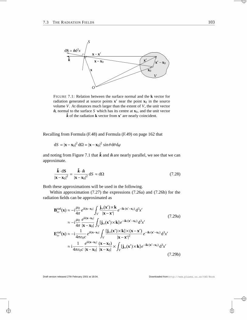
“main”2001/2/27page 103

7.3 THE RADIATION FIELDS 103

x−x′

x′

x0

O

dS = nd2x

kx′−x0

S

x−x0

x

V

FIGURE 7.1: Relation between the surface normal and the k vector forradiation generated at source points x′ near the point x0 in the sourcevolume V . At distances much larger than the extent of V , the unit vectorn, normal to the surface S which has its centre at x0, and the unit vector

k of the radiation k vector from x′ are nearly coincident.

Recalling from Formula (F.48) and Formula (F.49) on page 162 that

dS = |x−x0|2 dΩ = |x−x0|2 sinθdθdϕ

and noting from Figure 7.1 that k and n are nearly parallel, we see that we canapproximate.

k ·dS

|x−x0|2=

k · n|x−x0|2

dS ≈ dΩ (7.28)

Both these approximations will be used in the following.Within approximation (7.27) the expressions (7.26a) and (7.26b) for the

radiation fields can be approximated as

Bradω (x) ≈ −i

µ0

4πeik|x−x0 | V

jω(x′)×k|x−x′| e−ik·(x′−x0) d3x′

≈ −iµ0

4πeik|x−x0 |

|x−x0| V[jω(x′)×k]e−ik·(x′−x0) d3x′

(7.29a)

Eradω (x) ≈ −i

14πε0c

eik|x−x0 | V

[jω(x′)×k]× (x−x′)|x−x′|2 e−ik·(x′−x0) d3x′

≈ i1

4πε0ceik|x−x0 |

|x−x0|(x−x0)|x−x0| × V

[jω(x′)×k]e−ik·(x′−x0) d3x′

(7.29b)


“main”2001/2/27page 104


I.e., if max |x′−x0| |x−x′|, then the fields can be approximated as sphericalwaves multiplied by dimensional and angular factors, with integrals over pointsin the source volume only.

7.4 Radiated EnergyLet us consider the energy that is carried in the radiation fields Brad, Equa-tion (7.26a), and Erad, Equation (7.26b) on page 102. We have to treat signalswith limited lifetime and hence finite frequency bandwidth differently frommonochromatic signals.

7.4.1 Monochromatic signalsIf the source is strictly monochromatic, we can obtain the temporal average ofthe radiated power P directly, simply by averaging over one period so that

〈S〉 = 〈E×H〉 =1

2µ0Re 2 E×B∗ 3 =

12µ0

Re 2 Eωe−iωt × (Bωe−iωt)∗ 3=

12µ0

Re 2 Eω×B∗ω e−iωteiωt 3 =1

2µ0Re 2 Eω×B∗ω

3 (7.30)

Using the far-field approximations (7.29a) and (7.29b) and the fact that 1/c =√ε0µ0 and R0 =

√µ0/ε0 according to the definition (2.18) on page 26, we ob-

tain

〈S〉 = 132π2 R0

1

|x−x0|2 V

(jω×k)e−ik·(x′−x0) d3x′ 2 x−x0

|x−x0| (7.31)

or, making use of (7.28) on the preceding page,

dPdΩ

=1

32π2 R0

V(jω×k)e−ik·(x′−x0) d3x′

2 (7.32)

which is the radiated power per unit solid angle.

7.4.2 Finite bandwidth signalsA signal with finite pulse width in time (t) domain has a certain spread in fre-quency (ω) domain. To calculate the total radiated energy we need to integrate


“main”2001/2/27page 105

7.4 RADIATED ENERGY 105

over the whole bandwidth. The total energy transmitted through a unit area isthe time integral of the Poynting vector: ∞−∞S(t)dt = ∞−∞(E×H)dt

= ∞−∞ dω ∞−∞ dω′ ∞−∞(Eω×Hω′)e−i(ω+ω′)t dt

(7.33)

If we carry out the temporal integration first and use the fact that ∞−∞ e−i(ω+ω′)t dt = 2πδ(ω+ω′) (7.34)

Equation (7.33) above can be written [cf. Parseval’s identity] ∞−∞S(t)dt = 2π ∞−∞(Eω×H−ω)dω

= 2π ∞0 (Eω×H−ω)dω+ 0

−∞(Eω×H−ω)dω

= 2π ∞0 (Eω×H−ω)dω− −∞0(Eω×H−ω)dω

= 2π ∞0 (Eω×H−ω)dω+ ∞0 (E−ω×Hω)dω =

2πµ0 ∞0 (Eω×B−ω + E−ω×Bω)dω

=2πµ0 ∞0 (Eω×B∗ω + E∗ω×Bω)dω

(7.35)

where the last step follows from the real-valuedness of Eω and Bω. We in-sert the Fourier transforms of the field components which dominate at largedistances, i.e., the radiation fields (7.26a) and (7.26b). The result, after inte-gration over the area S of a large sphere which encloses the source, is

U =1

4π µ0

ε0 S ∞0 V

jω×k|x−x′|e

ik|x−x′ | d3x′ 2 k · ndS dω (7.36)

Inserting the approximations (7.27) and (7.28) into Equation (7.36) andalso introducing

U = ∞0 Uω dω (7.37)

and recalling the definition (2.18) on page 26 for the vacuum resistance R0 weobtain

dUω

dΩdω ≈ 1

4πR0

V(jω×k)e−ik·(x′−x0) d3x′

2 dω (7.38)


“main”2001/2/27page 106


which, at large distances, is a good approximation to the energy that is radiatedper unit solid angle dΩ in a frequency band dω. It is important to notice thatFormula (7.38) includes only source coordinates. This means that the amountof energy that is being radiated is independent on the distance to the source (aslong as it is large).

Bibliography[1] F. HOYLE, SIR AND J. V. NARLIKAR, Lectures on Cosmology and Action at a

Distance Electrodynamics, World Scientific Publishing Co. Pte. Ltd, Singapore,New Jersey, London and Hong Kong, 1996, ISBN 9810-02-2573-3(pbk).





[6] J. A. WHEELER AND R. P. FEYNMAN, Interaction with the absorber as a mech-anism for radiation, Reviews of Modern Physics, 17 (1945), pp. 157–.


“main”2001/2/27page 107

8Electromagnetic

Radiation andRadiating

Systems

In Chapter 3 we were able to derive general expressions for the scalar and vec-tor potentials from which we then, in Chapter 7, calculated the total electricand magnetic fields from arbitrary distributions of charge and current sources.The only limitation in the calculation of the fields was that the advanced po-tentials were discarded.

Thus, one can, at least in principle, calculate the radiated fields, Poyntingflux and energy for an arbitrary current density Fourier component and thenadd these Fourier components together to construct the complete electromag-netic field at any time at any point in space. However, in practice, it is oftendifficult to evaluate the source integrals unless the current has a simple distri-bution in space. In the general case, one has to resort to approximations. Weshall consider both these situations.

8.1 Radiation from Extended SourcesCertain radiation systems have a geometry which is one-dimensional, symmet-ric or in any other way simple enough that a direct calculation of the radiatedfields and energy is possible. This is for instance the case when the currentflows in one direction in space only and is limited in extent. An example ofthis is a linear antenna.

107

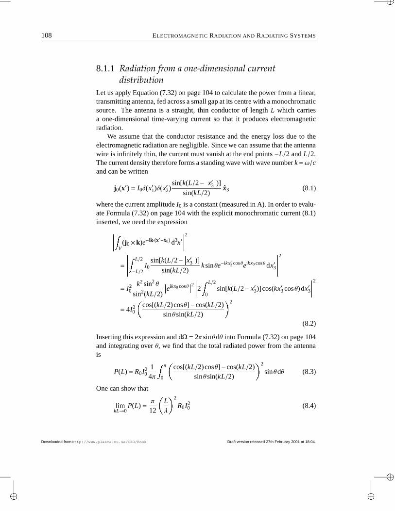
“main”2001/2/27page 108

108 ELECTROMAGNETIC RADIATION AND RADIATING SYSTEMS

8.1.1 Radiation from a one-dimensional currentdistribution

Let us apply Equation (7.32) on page 104 to calculate the power from a linear,transmitting antenna, fed across a small gap at its centre with a monochromaticsource. The antenna is a straight, thin conductor of length L which carriesa one-dimensional time-varying current so that it produces electromagneticradiation.

We assume that the conductor resistance and the energy loss due to theelectromagnetic radiation are negligible. Since we can assume that the antennawire is infinitely thin, the current must vanish at the end points −L/2 and L/2.The current density therefore forms a standing wave with wave number k =ω/cand can be written

j0(x′) = I0δ(x′1)δ(x′2)sin[k(L/2−

x′3 )]sin(kL/2)

x3 (8.1)

where the current amplitude I0 is a constant (measured in A). In order to evalu-ate Formula (7.32) on page 104 with the explicit monochromatic current (8.1)inserted, we need the expression V

(j0×k)e−ik·(x′−x0) d3x′ 2

=

L/2

−L/2I0

sin[k(L/2− x′3 )]

sin(kL/2)k sinθe−ikx′3 cosθeikx0 cosθ dx′3

2= I2

0k2 sin2 θ

sin2(kL/2)

eikx0 cosθ 2 2 L/2

0sin[k(L/2− x′3)]cos(kx′3 cosθ)dx′3

2= 4I2

0 cos[(kL/2)cosθ]− cos(kL/2)sinθ sin(kL/2) 2

(8.2)

Inserting this expression and dΩ = 2πsinθdθ into Formula (7.32) on page 104and integrating over θ, we find that the total radiated power from the antennais

P(L) = R0I20

14π π

0 cos[(kL/2)cosθ]− cos(kL/2)

sinθ sin(kL/2) 2

sinθdθ (8.3)

One can show that

limkL→0

P(L) =π

12 Lλ 2

R0I20 (8.4)


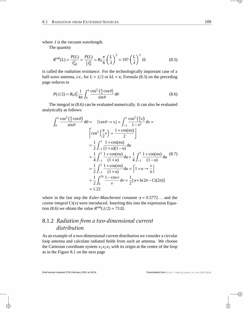
“main”2001/2/27page 109

8.1 RADIATION FROM EXTENDED SOURCES 109

where λ is the vacuum wavelength.The quantity

Rrad(L) =P(L)

I2eff

=P(L)12 I2

0

= R0π

6 Lλ 2

≈ 197 Lλ 2

Ω (8.5)

is called the radiation resistance. For the technologically important case of ahalf-wave antenna, i.e., for L = λ/2 or kL = π, Formula (8.3) on the precedingpage reduces to

P(λ/2) = R0I20

14π π

0

cos2 4 π2 cosθ 5sinθ

dθ (8.6)

The integral in (8.6) can be evaluated numerically. It can also be evaluatedanalytically as follows: π

0

cos2 4 π2 cosθ 5sinθ

dθ = dcosθ→ vc = 1

−1

cos2 4 π2 v 51− v2 dv =a

cos2 / π2

v 0 =1 + cos(πu)

2 b=

12 1

−1

1 + cos(πu)(1 + u)(1−u)

du

=14 1

−1

1 + cos(πu)(1 + u)

du +14 1

−1

1 + cos(πu)(1−u)

du

=12 1

−1

1 + cos(πu)(1 + u)

du = c 1 + u→ vπ d

=12 2π

0

1− cosvv

dv =12

[γ+ ln2π−Ci(2π)]

≈ 1.22

(8.7)

where in the last step the Euler-Mascheroni constant γ = 0.5772 . . . and thecosine integral Ci(x) were introduced. Inserting this into the expression Equa-tion (8.6) we obtain the value Rrad(λ/2) ≈ 73 Ω.

8.1.2 Radiation from a two-dimensional currentdistribution

As an example of a two-dimensional current distribution we consider a circularloop antenna and calculate radiated fields from such an antenna. We choosethe Cartesian coordinate system x1x2x3 with its origin at the centre of the loopas in the Figure 8.1 on the next page


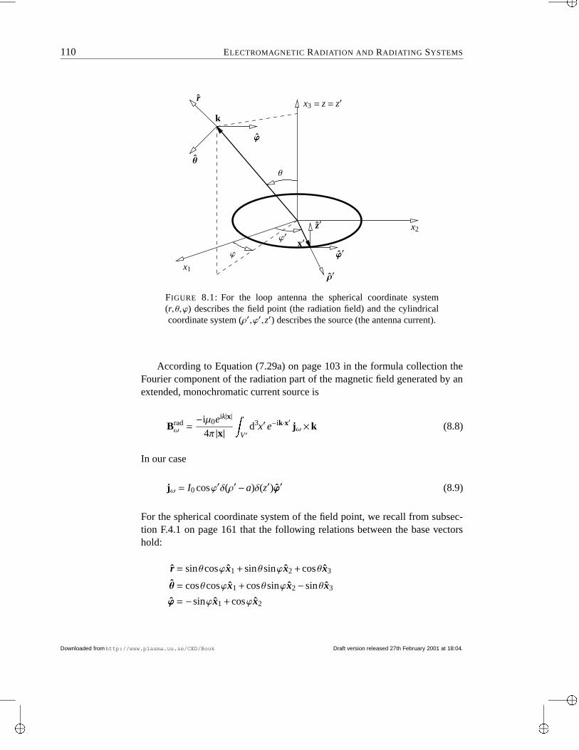
“main”2001/2/27page 110


x′

k

ϕ ϕ′

ρ′

θ

ϕ′

ϕ

r

x1

z′

θ

x3 = z = z′

x2

FIGURE 8.1: For the loop antenna the spherical coordinate system(r, θ,ϕ) describes the field point (the radiation field) and the cylindricalcoordinate system (ρ′,ϕ′,z′) describes the source (the antenna current).

According to Equation (7.29a) on page 103 in the formula collection theFourier component of the radiation part of the magnetic field generated by anextended, monochromatic current source is

Bradω =

−iµ0eik|x|

4π |x| V′d3x′ e−ik·x′ jω×k (8.8)

In our case

jω = I0 cosϕ′δ(ρ′−a)δ(z′)ϕ′ (8.9)

For the spherical coordinate system of the field point, we recall from subsec-tion F.4.1 on page 161 that the following relations between the base vectorshold:

r = sinθcosϕx1 + sinθ sinϕx2 + cosθx3

θ = cosθcosϕx1 + cosθ sinϕx2− sinθx3

ϕ = −sinϕx1 + cosϕx2


“main”2001/2/27page 111

8.1 RADIATION FROM EXTENDED SOURCES 111

and

x1 = sinθcosϕr + cosθcosϕθ− sinϕϕ

x2 = sinθ sinϕr + cosθ sinϕθ+ cosϕϕ

x3 = cosθ r− sinθθ

With the use of the above transformations and trigonometric identities, weobtain for the cylindrical coordinate system which describes the source:

ρ′ = cosϕ′ x1 + sinϕ′ x2

= sinθcos(ϕ′−ϕ)r + cosθcos(ϕ′−ϕ)θ+ sin(ϕ′−ϕ)ϕ(8.10)

ϕ′ = −sinϕ′ x1 + cosϕ′ x2

= −sinθ sin(ϕ′−ϕ)r− cosθ sin(ϕ′−ϕ)θ+ cos(ϕ′−ϕ)ϕ(8.11)

z′ = x3 = cosθ r− sinθθ (8.12)

This choice of coordinate systems means that k = k r and x′ = aρ′ so that

k ·x′ = kasinθcos(ϕ′−ϕ) (8.13)

and

ϕ′×k = k[cos(ϕ′−ϕ)θ+ cosθ sin(ϕ′−ϕ)ϕ] (8.14)

With these expressions inserted and d3x′ = ρ′dρ′dϕ′dz′, the source integralbecomes

V′d3x′ e−ik·x′ jω×k = a 2π

0dϕ′ e−ikasinθcos(ϕ′−ϕ)I0 cosϕ′ ϕ×k

= I0ak 2π

0e−ikasinθcos(ϕ′−ϕ) cos(ϕ′−ϕ)cosϕ′ dϕ′ θ

+ I0ak cosθ 2π

0e−ikasinθcos(ϕ′−ϕ) sin(ϕ′−ϕ)cosϕ′ dϕ′ ϕ

(8.15)

Utilising the periodicity of the integrands over the integration interval [0,2π],introducing the auxiliary integration variable ϕ′′ = ϕ′−ϕ, and utilising standard


“main”2001/2/27page 112


trigonometric identities, the first integral in the RHS of (8.15) can be rewritten

2π

0e−ikasinθcosϕ′′ cosϕ′′ cos(ϕ′′+ϕ)dϕ′′

= cosϕ 2π

0e−ikasinθcosϕ′′ cos2ϕ′′ dϕ′′ + a vanishing integral

= cosϕ 2π

0e−ikasinθcosϕ′′ 1

2+

12

cos2ϕ′′ dϕ′′

=12

cosϕ 2π

0e−ikasinθcosϕ′′ dϕ′′

+12

cosϕ 2π

0e−ikasinθcosϕ′′ cos2ϕ′′ dϕ′′

(8.16)

Analogously, the second integral in the RHS of (8.15) can be rewritten

2π

0e−ikasinθcosϕ′′ sinϕ′′ cos(ϕ′′+ϕ)dϕ′′

=12

sinϕ 2π

0e−ikasinθcosϕ′′ dϕ′′

− 12

sinϕ 2π

0e−ikasinθcosϕ′′ cos2ϕ′′ dϕ′′

(8.17)

As is well-known from the theory of Bessel functions,

Jn(−ξ) = (−1)nJn(ξ)

Jn(−ξ) =i−n

π π

0e−iξ cosϕ cosnϕdϕ =

i−n

2π 2π

0e−iξ cosϕ cosnϕdϕ

(8.18)

which means that 2π

0e−ikasinθcosϕ′′ dϕ′′ = 2πJ0(kasinθ) 2π

0e−ikasinθcosϕ′′ cos2ϕ′′ dϕ′′ = −2πJ2(kasinθ)

(8.19)

Putting everything together, we find that V′d3x′ e−ik·x′ jω×k = Iθ θ+Iϕ ϕ

= I0akπcosϕ [J0(kasinθ)− J2(kasinθ)] θ

+ I0akπcosθ sinϕ [J0(kasinθ) + J2(kasinθ)] ϕ

(8.20)


“main”2001/2/27page 113

8.2 MULTIPOLE RADIATION 113

so that, in spherical coordinates where |x| = r,

Bradω (x) =

−iµ0eikr

4πr 4 Iθ θ+Iϕ ϕ 5 (8.21)

To obtain the desired physical magnetic field in the radiation (far) zone wemust Fourier transform back to t space and take the real part and evaluate it atthe retarded time:

Brad(t,x) = Re −iµ0e(ikr−ωt′)

4πr 4 Iθ θ+Iϕ ϕ 5 =µ0

4πrsin(kr−ωt′) 4 Iθ θ+Iϕ ϕ 5

=I0akµ0

4rsin(kr−ωt′) cosϕ [J0(kasinθ)− J2(kasinθ)] θ

+ cosθ sinϕ [J0(kasinθ) + J2(kasinθ)] ϕ (8.22)

From this expression for the radiated B field, we can obtain the radiated E fieldwith the help of Maxwell’s equations.

8.2 Multipole RadiationIn the general case, and when we are interested in evaluating the radiation farfrom the source volume, we can introduce an approximation which leads to amultipole expansion where individual terms can be evaluated analytically. Weshall use Hertz’ method to obtain this expansion.

8.2.1 The Hertz potentialLet us consider the continuity equation, which, according to expression (1.21)on page 9, can be written

∂ρ(t,x)∂t

+∇ · j(t,x) = 0 (8.23)

If we introduce a vector field π(t,x) such that

∇ ·π = −ρtrue (8.24a)

∂π

∂t= jtrue (8.24b)


“main”2001/2/27page 114


and compare with Equation (8.23) on the previous page, we see that π(t,x)satisfies this continuity equation. Furthermore, if we compare with the electricpolarisation [cf. Equation (6.9) on page 87], we see that the quantity π isrelated to the “true” charges in the same way as P is related to polarised charge.Therefore, π is referred to as the polarisation vector.

We introduce a further potential Πe with the following property

∇ ·Πe = −φ (8.25a)

1c2

∂Πe

∂t= A (8.25b)

where φ and A are the electromagnetic scalar and vector potentials, respec-tively. As we see, Πe acts as a “super-potential” in the sense that it is a poten-tial from which we can obtain other potentials. It is called the Hertz’ vectoror polarisation potential and, as can be seen from (8.24) and (8.25), it satisfiesthe inhomogeneous wave equation6 2Πe =

1c2

∂2

∂t2 Πe−∇2Πe =π

ε0(8.26)

This equation is of the same type as Equation (3.20) on page 40, and hastherefore the retarded solution

Πe(t,x) =1

4πε0 π(t′ret,x′)

|x−x′| d3x′ (8.27)

with Fourier components

Πeω(x) =

14πε0 πω(x′)eik|x−x′ |

|x−x′| d3x′ (8.28)

If we introduce the help vector C such that

C = ∇×Πe (8.29)

we see that we can calculate the magnetic and electric fields, respectively, asfollows

B =1c2

∂C∂t

(8.30a)

E = ∇×C (8.30b)

Clearly, the last equation is valid only outside the source volume, where∇ ·E = 0. Since we are mainly interested in the fields in the far zone, a longdistance from the source region, this is no essential limitation.


“main”2001/2/27page 115


Assume that the source region is a limited volume around some centralpoint x0 far away from the field (observation) point x. Under these assump-tions, we can expand expression (8.27) on the facing page the Hertz’ vector,due to the presence of non-vanishing π(t′ret,x

′) in the vicinity of x0, in a formalseries. For this purpose we recall from potential theory that

eik|x−x′ |

|x−x′| ≡eik|(x−x0)−(x′−x0)|

|(x−x0)− (x′−x0)|= ik

∞∑n=0

(2n + 1)Pn(cosΘ) jn(k x′−x0

)h(1)n (k |x−x0|)

(8.31)

where

eik|x−x′ |

|x−x′| is a Green´s function

Θ is the angle between x′−x0 and x−x0

Pn(cosΘ) is the Legendre polynomial of order n

jn(k x′−x0

) is the spherical Bessel function of the first kind of order n

h(1)n (k |x−x0|) is the spherical Hankel function of the first kind of order n

According to the addition theorem for Legendre polynomials, we can write

Pn(cosΘ) =n

∑m=−n

(−1)mPmn (cosθ)P−m

n (cosθ′)eim(ϕ−ϕ′) (8.32)

where Pmn is an associated Legendre polynomial and, in spherical polar coor-

dinates,

x′−x0 = ( x′−x0

, θ′,φ′) (8.33a)

x−x0 = (|x−x0| , θ,φ) (8.33b)

Inserting Equation (8.31) above, together with Equation (8.32), into Equa-tion (8.28) on the preceding page, we can in a formally exact way expandthe Fourier component of the Hertz’ vector as

Πeω =

ik4πε0

∞∑n=0

n

∑m=−n

(2n + 1)(−1)mh(1)n (k |x−x0|) Pm

n (cosθ)eimϕ

× Vπω(x′) jn(k

x′−x0

) P−mn (cosθ′)e−imϕ′ d3x′

(8.34)

We notice that there is no dependence on x− x0 inside the integral; the inte-grand is only dependent on the relative source vector x′−x0.


“main”2001/2/27page 116


We are interested in the case where the field point is many wavelengthsaway from the well-localised sources, i.e., when the following inequalities

k x′−x0

1 k |x−x0| (8.35)

hold. Then we may to a good approximation replace h(1)n with the first term in

its asymptotic expansion:

h(1)n (k |x−x0|) ≈ (−i)n+1 eik|x−x0 |

k |x−x0| (8.36)

and replace jn with the first term in its power series expansion:

jn(k x′−x0

) ≈ 2nn!(2n + 1)! 4 k x′−x0

5 n(8.37)

Inserting these expansions into Equation (8.34) on the preceding page, we ob-tain the multipole expansion of the Fourier component of the Hertz’ vector

Πeω ≈

∞∑n=0

Πeω

(n) (8.38a)

where

Πeω

(n) = (−i)n 14πε0

eik|x−x0 |

|x−x0|2nn!(2n)! V

πω(x′) (k x′−x0

)n Pn(cosΘ)d3x′ (8.38b)

This expression is approximately correct only if certain care is exercised; ifmany Πe

ω(n) terms are needed for an accurate result, the expansions of the

spherical Hankel and Bessel functions used above may not be consistent andmust be replaced by more accurate expressions. Taking the inverse Fouriertransform of Πe

ω will yield the Hertz’ vector in time domain, which insertedinto Equation (8.29) on page 114 will yield C. The resulting expression canthen in turn be inserted into Equation (8.30) on page 114 in order to obtain theradiation fields.

For a linear source distribution along the polar axis, Θ = θ in expres-sion (8.38b) above, and Pn(cosθ) gives the angular distribution of the radia-tion. In the general case, however, the angular distribution must be computedwith the help of Formula (8.32) on the preceding page. Let us now study thelowest order contributions to the expansion of Hertz’ vector.


“main”2001/2/27page 117


8.2.2 Electric dipole radiationChoosing n = 0 in expression (8.38b) on the preceding page, we obtain

Πeω

(0) =eik|x−x0 |

4πε0 |x−x0| Vπω(x′)d3x′ =

14πε0

eik|x−x0 |

|x−x0| pω (8.39)

where pω = V πω(x′)d3x′ is the Fourier component of the electric dipole mo-ment; cf. Equation (6.2) on page 85 which describes the static dipole moment.If a spherical coordinate system is chosen with its polar axis along pω, thecomponents of Πe

ω(0) are

Πer = Πe(0)

ω cosθ =1

4πε0

eik|x−x0 |

|x−x0| pω cosθ (8.40a)

Πeθ = −Πe(0)

ω sinθ = − 14πε0

eik|x−x0 |

|x−x0| pω sinθ (8.40b)

Πeϕ = 0 (8.40c)

Evaluating Formula (8.29) on page 114 for the help vector C, with thespherically polar components (8.40) of Πe(0)

ω inserted, we obtain

Cω = C(0)ω,ϕ φ =

14πε0

1|x−x0| − ik eik|x−x0 |

|x−x0| pω sinθ φ (8.41)

Applying this to Equation (8.30) on page 114, we obtain directly the Fouriercomponents of the fields

Bω = −iωµ0

4π 1|x−x0| − ik eik|x−x0 |

|x−x0| pω sinθ φ (8.42a)

Eω =1

4πε0 2 1

|x−x0|2− ik|x−x0| cosθ

x−x0

|x−x0|

+ 1

|x−x0|2− ik|x−x0| − k2 sinθ θ eik|x−x0 |

|x−x0| pω(8.42b)

Keeping only those parts of the fields which dominate at large distances(the radiation fields) and recalling that the wave vector k = k(x− x0)/ |x−x0|where k =ω/c, we can now write down the Fourier components of the radiationparts of the magnetic and electric fields from the dipole:

Bradω = −ωµ0

4πeik|x−x0 |

|x−x0| (pω×k) (8.43a)

Eradω = − 1

4πε0

eik|x−x0 |

|x−x0| [(pω×k)×k] (8.43b)


“main”2001/2/27page 118


These fields constitute the electric dipole radiation, also known as E1 radia-tion.

8.2.3 Magnetic dipole radiationThe next term in the expression (8.38b) on page 116 for the expansion of theFourier transform of the Hertz’ vector is for n = 1:

Πeω

(1) = −ieik|x−x0 |

4πε0 |x−x0| Vk x′−x0

πω(x′)cosΘd3x′

= −ik1

4πε0

eik|x−x0 |

|x−x0|2 V[(x−x0) · (x′−x0)]πω(x′)d3x′

(8.44)

Here, the term [(x−x0) · (x′−x0)]πω(x′) can be rewritten

[(x−x0) · (x′−x0)]πω(x′) = (xi− x0,i)(x′i − x0,i)πω(x′) (8.45)

and introducing

ηi = xi− x0,i (8.46a)

η′i = x′i − x0,i (8.46b)

the jth component of the integrand in Πeω

(1) can be broken up into

[(x−x0) · (x′−x0)]πω(x′) j =12ηi 4 πω, jη′i +πω,iη

′j5

+12ηi 4 πω, jη′i −πω,iη′j 5 (8.47)

i.e., as the sum of two parts, the first being symmetric and the second antisym-metric in the indices i, j. We note that the antisymmetric part can be writtenas

12ηi 4 πω, jη′i −πω,iη′j 5 =

12

[πω, j(ηiη′i)−η′j(ηiπω,i)]

=12

[πω(η ·η′)−η′(η ·πω)] j

=122 (x−x0)× [πω× (x′−x0)] 3 j

(8.48)

The utilisation of Equations (8.24) on page 113, and the fact that we areconsidering a single Fourier component,

π(t,x) = πωe−iωt (8.49)


“main”2001/2/27page 119


allow us to express πω in jω as

πω = ijωω

(8.50)

Hence, we can write the antisymmetric part of the integral in Formula (8.44)on the preceding page as

12

(x−x0)× Vπω(x′)× (x′−x0)d3x′

= i1

2ω(x−x0)× V

jω(x′)× (x′−x0)d3x′

= −i1ω

(x−x0)×mω

(8.51)

where we introduced the Fourier transform of the magnetic dipole moment

mω =12 V

(x′−x0)× jω(x′)d3x′ (8.52)

The final result is that the antisymmetric, magnetic dipole, part of Πeω

(1)

can be written

Πe,antisymω

(1)= − k

4πε0ω

eik|x−x0 |

|x−x0|2(x−x0)×mω (8.53)

In analogy with the electric dipole case, we insert this expression into Equa-tion (8.29) on page 114 to evaluate C, with which Equations (8.30) on page 114then gives the B and E fields. Discarding, as before, all terms belonging to thenear fields and transition fields and keeping only the terms that dominate atlarge distances, we obtain

Bradω (x) = −µ0

4πeik|x−x0 |

|x−x0| (mω×k)×k (8.54a)

Eradω (x) =

k4πε0c

eik|x−x0 |

|x−x0| mω×k (8.54b)

which are the fields of the magnetic dipole radiation (M1 radiation).

8.2.4 Electric quadrupole radiation

The symmetric part Πe,symω

(1)of the n = 1 contribution in the Equation (8.38b)

on page 116 for the expansion of the Hertz’ vector can be expressed in terms


“main”2001/2/27page 120


of the electric quadrupole tensor, which is defined in accordance with Equa-tion (6.3) on page 86:

Q(t) = V(x′−x0)(x′−x0)ρ(t,x′)d3x′ (8.55)

Again we use this expression in Equation (8.29) on page 114 to calculate thefields via Equations (8.30) on page 114. Tedious, but fairly straightforwardalgebra (which we will not present here), yields the resulting fields. The ra-diation components of the fields in the far field zone (wave zone) are givenby

Bradω (x) =

iµ0ω

8πeik|x−x0 |

|x−x0| 4 k ·Qω5 ×k (8.56a)

Eradω (x) =

i8πε0

eik|x−x0 |

|x−x0| 4 k ·Qω5 ×k ×k (8.56b)

This type of radiation is called electric quadrupole radiation or E2 radiation.

8.3 Radiation from a Localised Charge inArbitrary Motion

The derivation of the radiation fields for the case of the source moving rela-tive to the observer is considerably more complicated than the stationary casesstudied above. In order to handle this non-stationary situation, we use the re-tarded potentials (3.37) on page 44 in Chapter 3

φ(t,x) =1

4πε0 V

ρ(t′ret,x′)

|x−x′| d3x′ (8.57a)

A(t,x) =µ0

4π V

j(t′ret,x′)

|x−x′| d3x′ (8.57b)

and consider a source region with such a limited spatial extent that the chargesand currents are well localised. Specifically, we consider a charge q′, for in-stance an electron, which, classically, can be thought of as a localised, unstruc-tured and rigid “charge distribution” with a small, finite radius. The part of this“charge distribution” dq′ which we are considering is located in dV ′ = d3x′ inthe sphere in Figure 8.2 on the next page. Since we assume that the electron(or any other other similar electric charge) is moving with a velocity v whosedirection is arbitrary and whose magnitude can be almost comparable to thespeed of light, we cannot say that the charge and current to be used in (8.57) is


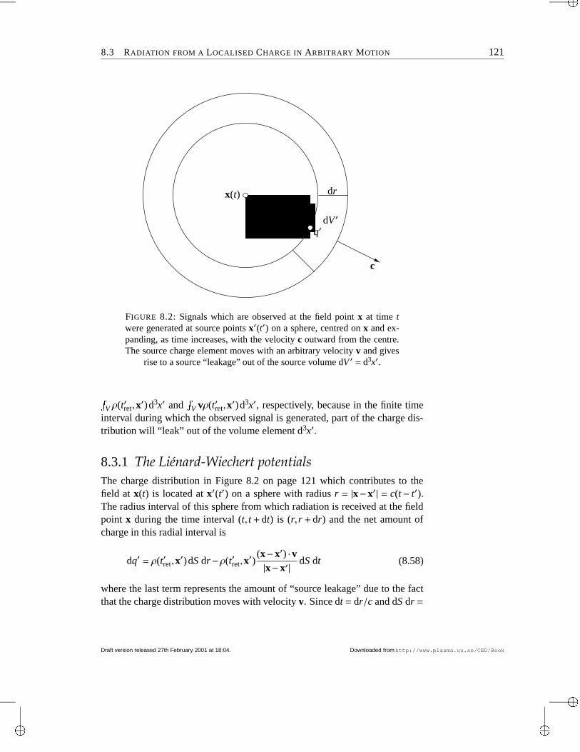
“main”2001/2/27page 121

8.3 RADIATION FROM A LOCALISED CHARGE IN ARBITRARY MOTION 121

efefefeefefefegfgfgfggfgfgfghfhfhfhfhfhfhfhfhhfhfhfhfhfhfhfhfhhfhfhfhfhfhfhfhfhififififififififiififififififififiififififififififiv

x′(t′)

dSdV ′

drx(t)

q′x−x′

c

FIGURE 8.2: Signals which are observed at the field point x at time twere generated at source points x′(t′) on a sphere, centred on x and ex-panding, as time increases, with the velocity c outward from the centre.The source charge element moves with an arbitrary velocity v and gives

rise to a source “leakage” out of the source volume dV ′ = d3x′.

V ρ(t′ret,x′)d3x′ and V vρ(t′ret,x

′)d3x′, respectively, because in the finite timeinterval during which the observed signal is generated, part of the charge dis-tribution will “leak” out of the volume element d3x′.

8.3.1 The Liénard-Wiechert potentialsThe charge distribution in Figure 8.2 on page 121 which contributes to thefield at x(t) is located at x′(t′) on a sphere with radius r = |x−x′| = c(t− t′).The radius interval of this sphere from which radiation is received at the fieldpoint x during the time interval (t, t + dt) is (r,r + dr) and the net amount ofcharge in this radial interval is

dq′ = ρ(t′ret,x′)dS dr−ρ(t′ret,x

′)(x−x′) ·v|x−x′| dS dt (8.58)

where the last term represents the amount of “source leakage” due to the factthat the charge distribution moves with velocity v. Since dt = dr/c and dS dr =


“main”2001/2/27page 122


d3x′ we can rewrite this expression for the net charge as

dq′ = ρ(t′ret,x′)d3x′−ρ(t′ret,x

′)(x−x′) ·vc |x−x′| d3x′

= ρ(t′ret,x′) 1− (x−x′) ·v

c |x−x′| d3x′(8.59)

or

ρ(t′ret,x′)d3x′ =

dq′

1− (x−x′)·vc|x−x′ |

(8.60)

which leads to the expression

ρ(t′ret,x′)

|x−x′| d3x′ =dq′

|x−x′| − (x−x′)·vc

(8.61)

This is the expression to be used in the Formulae (8.57) on page 120 for theretarded potentials. The result is (recall that j = ρv)

φ(t,x) =1

4πε0 dq′

|x−x′| − (x−x′)·vc

(8.62a)

A(t,x) =µ0

4π vdq′

|x−x′| − (x−x′)·vc

(8.62b)

For a sufficiently small and well localised charge distribution we can, assumingthat the integrands do not change sign in the integration volume, use the meanvalue theorem and the fact that V dq′ = q′ to evaluate these expressions tobecome

φ(t,x) =q′

4πε0

1

|x−x′| − (x−x′)·vc

=q′

4πε0

1s

(8.63a)

A(t,x) =q′

4πε0c2

v

|x−x′| − (x−x′)·vc

=q′

4πε0c2

vs

=vc2 φ(t,x) (8.63b)

where

s = x−x′

− (x−x′) ·vc

(8.64a)

= x−x′

1− x−x′

|x−x′| ·vc (8.64b)

= (x−x′) · x−x′

|x−x′| −vc (8.64c)


“main”2001/2/27page 123


is the retarded relative distance. The potentials (8.63) are precisely the Liénard-Wiechert potentials which we derived in Section 4.3.2 on page 60 by using acovariant formalism.

It is important to realise that in the complicated derivation presented here,the observer is in a coordinate system which has an “absolute” meaning and thevelocity v is that of the particle, whereas in the covariant derivation two framesof equal standing were moving relative to each other with v. Expressed in thefour-potential, Equation (4.48) on page 59, the Liénard-Wiechert potentialsbecome

Aµ(xκ) =q′

4πε0 1

s,

vcs = (φ,cA) (8.65)

The Liénard-Wiechert potentials are applicable to all problems where aspatially localised charge emits electromagnetic radiation, and we shall nowstudy such emission problems. The electric and magnetic fields are calculatedfrom the potentials in the usual way:

B(t,x) = ∇×A(t,x) (8.66a)

E(t,x) = −∇φ(t,x)− ∂A(t,x)∂t

(8.66b)

8.3.2 Radiation from an accelerated point chargeConsider a localised charge q′ and assume that its trajectory is known experi-mentally as a function of retarded time

x′ = x′(t′) (8.67)

(in the interest of simplifying our notation, we drop the subscript “ret” on t′

from now on). This means that we know the trajectory of the charge q′, i.e., x′,for all times up to the time t′ at which a signal was emitted in order to preciselyarrive at the field point x at time t. Because of the finite speed of propagationof the fields, the trajectory at times later than t′ is not (yet) known.

The retarded velocity and acceleration at time t′ are given by

v(t′) =dx′

dt′(8.68a)

a(t′) = v(t′) =dvdt′

=d2x′

dt′2(8.68b)

As for the charge coordinate x′ itself, we have in general no knowledge of thevelocity and acceleration at times later than t′, in particular not at the time of


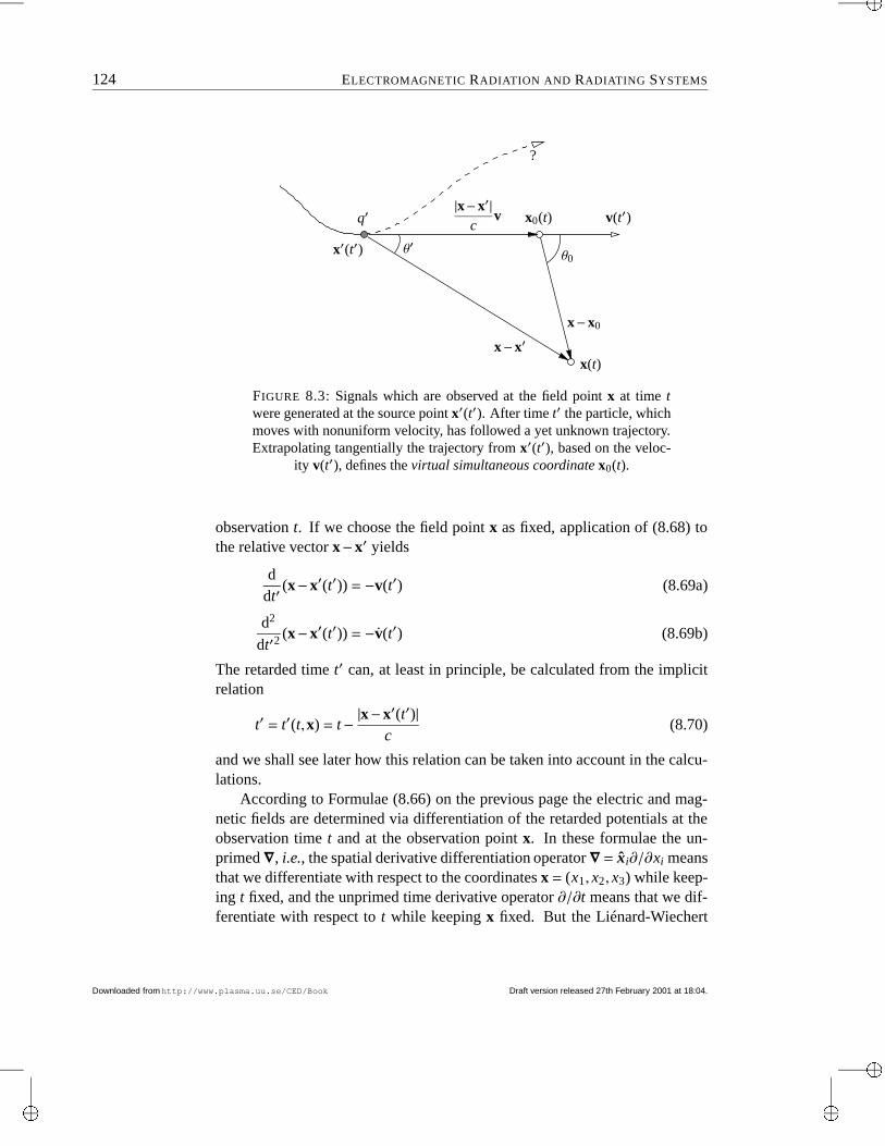
“main”2001/2/27page 124


v(t′)

x(t)

q′

x−x0

x−x′

x′(t′)

|x−x′|c

v x0(t)

θ0

?

θ′

FIGURE 8.3: Signals which are observed at the field point x at time twere generated at the source point x′(t′). After time t′ the particle, whichmoves with nonuniform velocity, has followed a yet unknown trajectory.Extrapolating tangentially the trajectory from x′(t′), based on the veloc-

ity v(t′), defines the virtual simultaneous coordinate x0(t).

observation t. If we choose the field point x as fixed, application of (8.68) tothe relative vector x−x′ yields

ddt′

(x−x′(t′)) = −v(t′) (8.69a)

d2

dt′2(x−x′(t′)) = −v(t′) (8.69b)

The retarded time t′ can, at least in principle, be calculated from the implicitrelation

t′ = t′(t,x) = t− |x−x′(t′)|c

(8.70)

and we shall see later how this relation can be taken into account in the calcu-lations.

According to Formulae (8.66) on the previous page the electric and mag-netic fields are determined via differentiation of the retarded potentials at theobservation time t and at the observation point x. In these formulae the un-primed∇, i.e., the spatial derivative differentiation operator∇= xi∂/∂xi meansthat we differentiate with respect to the coordinates x = (x1, x2, x3) while keep-ing t fixed, and the unprimed time derivative operator ∂/∂t means that we dif-ferentiate with respect to t while keeping x fixed. But the Liénard-Wiechert


“main”2001/2/27page 125


potentials φ and A, Equations (8.63) on page 122, are expressed in the chargevelocity v(t′) given by Equation (8.68a) on page 123 and the retarded relativedistance s(t′,x) given by Equation (8.64) on page 122. This means that theexpressions for the potentials φ and A contain terms which are expressed ex-plicitly in t′, which in turn is expressed implicitly in t via Equation (8.70) onthe preceding page. Despite this complication it is possible, as we shall seebelow, to determine the electric and magnetic fields and associated quantitiesat the time of observation t. To this end, we need to investigate carefully theaction of differentiation on the potentials.

The differential operator method

We introduce the convention that a differential operator embraced by paren-theses with an index x or t means that the operator in question is applied atconstant x and t, respectively. With this convention, we find that ∂

∂t′ x

x−x′(t′) = x−x′

|x−x′| · ∂∂t′ x 4 x−x′(t′) 5 = − (x−x′) ·v|x−x′| (8.71)

Furthermore, by applying the operator (∂/∂t)x to Equation (8.70) on the facingpage we find that ∂t′

∂t x= 1− ∂

∂t x

|x−x′(t′(t,x))|c

= 1− j ∂∂t′ x

|x−x′|c ∂t′

∂t x

= 1 +(x−x′) ·vc |x−x′| ∂t′

∂t x

(8.72)

This is an algebraic equation in (∂t′/∂t)x which we can solve to obtain ∂t′

∂t x=

|x−x′||x−x′| − (x−x′) ·v/c =

|x−x′|s

(8.73)

where s = s(t′,x) is the retarded relative distance given by Equation (8.64)on page 122. Making use of Equation (8.73), we obtain the following usefuloperator identity ∂

∂t x= ∂t′

∂t x ∂∂t′ x

=|x−x′|

s ∂∂t′ x

(8.74)


“main”2001/2/27page 126


Likewise, by applying (∇)t to Equation (8.70) on page 124 we obtain

(∇)t t′ = −(∇)t|x−x′(t′(t,x))|

c= − x−x′

c |x−x′| · (∇)t(x−x′)

= − x−x′

c |x−x′| +(x−x′) ·vc |x−x′| (∇)t t′

(8.75)

This is an algebraic equation in (∇)t with the solution

(∇)tt′ = −x−x′

cs(8.76)

which gives the following operator relation when (∇)t is acting on an arbitraryfunction of t′ and x:

(∇)t = (∇)tt′ ∂

∂t′ x+ (∇)t′ = −x−x′

cs ∂∂t′ x

+ (∇)t′ (8.77)

With the help of the rules (8.77) and (8.74) we are now able to replace t by t′

in the operations which we need to perform. We find, for instance, that

∇φ ≡ (∇φ)t = ∇ 14πε0

q′

s = − q′

4πε0s2 x−x′

|x−x′| −vc− x−x′

cs ∂s∂t′ x (8.78a)

∂A∂t≡ ∂A

∂t x=∂

∂t µ0

4πq′vs

=q′

4πε0c2s3 x−x′ sv−

x−x′ v ∂s

∂t′ x (8.78b)

Utilising these relations in the calculation of the E field from the Liénard-Wiechert potentials, Equations (8.63) on page 122, we obtain

E(t,x) = −∇φ− ∂A∂t

=q′

4πε0s2 (x−x′)− |x−x′|v/c|x−x′|

− (x−x′)− |x−x′|v/ccs

∂s∂t′ x

− |x−x′| vc2 (8.79)

Starting from expression (8.64a) on page 122 for the retarded relative distance


“main”2001/2/27page 127


s(t′,x), we see that we can evaluate (∂s/∂t′)x in the following way ∂s∂t′ x

= ∂∂t′ x

x−x′ − (x−x′) ·v

c =

∂

∂t′ x−x′(t′)

− 1c _ ∂ 4 x−x′(t′) 5

∂t′·v− (x−x′) · ∂v(t′)

∂t′ `= − (x−x′) ·v

|x−x′| +v2

c− (x−x′) · v

c

(8.80)

where Equation (8.71) on page 125 and Equations (8.68) on page 123, respec-tively, were used. Hence, the electric field generated by an arbitrarily movingcharged particle at x′(t′) is given by the expression

E(t,x) =q′

4πε0s3 k (x−x′)− |x−x′|vc 1− v2

c2 M NFO PCoulomb field when v→ 0

+x−x′

c2 × l (x−x′)− |x−x′|vc × v M NFO P

Radiation field

(8.81)

The first part of the field, the velocity field, tends to the ordinary Coulomb fieldwhen v→ 0 and does not contribute to the radiation. The second part of thefield, the acceleration field, is radiated into the far zone and is therefore alsocalled the radiation field.

From Figure 8.3 on page 124 we see that the position the charged particlewould have had if at t′ all external forces would have been switched off so thatthe trajectory from then on would have been a straight line in the direction ofthe tangent at x′(t′) is x0(t), the virtual simultaneous coordinate. During thearbitrary motion, we interpret x−x0 as the coordinate of the field point x rela-tive to the virtual simultaneous coordinate x0(t). Since the time it takes from asignal to propagate (in the assumed vacuum) from x′(t′) to x is |x−x′|/c, thisrelative vector is given by

x−x0 = (x−x′)− |x−x′|vc

(8.82)

This allows us to rewrite Equation (8.81) above in the following way

E(t,x) =q′

4πε0s3 (x−x0) 1− v2

c2 + (x−x′)× (x−x0)× vc2 (8.83)


“main”2001/2/27page 128


In a similar manner we can compute the magnetic field:

B(t,x) = ∇×A ≡ (∇)t ×A = (∇)t′ ×A− x−x′

cs× ∂

∂t′ xA

= − q′

4πε0c2s2

x−x′

|x−x′| ×v− x−x′

c |x−x′| × ∂A∂t x

(8.84)

where we made use of Equation (8.63) on page 122 and Formula (8.74) onpage 125. But, according to (8.78a),

x−x′

c |x−x′| × (∇)tφ =q′

4πε0c2s2

x−x′

|x−x′| ×v (8.85)

so that

B(t,x) =x−x′

c |x−x′| × −(∇φ)t − ∂A∂t x

=x−x′

c |x−x′| ×E(t,x)

(8.86)

The radiation part of the electric field is obtained from the accelerationfield in Formula (8.81) on the preceding page as

Erad(t,x) = lim|x−x′ |→∞

E(t,x)

=q′

4πε0c2s3 (x−x′)× l (x−x′)− |x−x′|vc × v

=q′

4πε0c2s3 (x−x′)× [(x−x0)× v]

(8.87)

where in the last step we again used Formula (8.82) on the previous page.Using this formula and Formula (8.86), the radiation part of the magnetic fieldcan be written

Brad(t,x) =x−x′

c |x−x′| ×Erad(t,x) (8.88)

The direct method An alternative to the differential operator transformationtechnique just described is to try to express all quantities in the potentials di-rectly in t and x. An example of such a quantity is the retarded relative distances(t′,x). According to Equation (8.64) on page 122, the square of this retardedrelative can be written

s2(t′,x) = x−x′

2−2 x−x′

(x−x′) ·vc

+ (x−x′) ·vc 2

(8.89)


“main”2001/2/27page 129


If we use the following handy identity (x−x′) ·vc 2

+ (x−x′)×vc 2

=|x−x′|2 v2

c2 cos2 θ′+|x−x′|2 v2

c2 sin2 θ′

=|x−x′|2 v2

c2 (cos2 θ′+ sin2 θ′) =|x−x′|2 v2

c2

(8.90)

we find that (x−x′) ·vc 2

=|x−x′|2 v2

c2 − (x−x′)×vc 2

(8.91)

Furthermore, from Equation (8.82) on page 127, we obtain the following iden-tity:

(x−x′)×v = (x−x0)×v (8.92)

which, when inserted into Equation (8.91) above, yields the relation (x−x′) ·vc 2

=|x−x′|2 v2

c2 − (x−x0)×vc 2

(8.93)

Inserting the above into expression (8.89) on the facing page for s2, thisexpression becomes

s2 = x−x′

2−2 x−x′

(x−x′) ·vc

+|x−x′|2 v2

c2 − (x−x0)×vc 2

= (x−x′)− |x−x′|vc 2

− (x−x0)×vc 2

= (x−x0(t))2− (x−x0(t))×vc 2

≡ |x−x0|2− (x−x0)×vc 2

(8.94)

where in the penultimate step we used Equation (8.82) on page 127.What we have just demonstrated is that, in the case the particle velocity at

time t can be calculated or projected, the retarded distance s in the Liénard-Wiechert potentials (8.63) can be expressed in terms of the virtual simultane-ous coordinate x0(t), viz., the point at which the particle will have arrived at


“main”2001/2/27page 130


time t, i.e., when we obtain the first knowledge of its existence at the sourcepoint x′ at the retarded time t′, and in the field coordinate x(t), where we makeour observations. We have, in other words, shown that all quantities in the def-inition of s, and hence s itself, can, when the motion of the charge is somehowknown, be expressed in terms of the time t alone. I.e., in this special case weare able to express the retarded relative distance as s = s(t,x) and we do nothave to involve the retarded time t′ or transformed differential operators in ourcalculations.

Taking the square root of both sides of Equation (8.94) on the precedingpage, we obtain the following alternative final expressions for the retarded rel-ative distance s in terms of the charge’s virtual simultaneous coordinate x0(t):

s(t,x) = |x−x0|2− (x−x0)×vc 2

(8.95a)

= |x−x0| 1− v2

c2 sin2 θ0 (8.95b)

= |x−x0|2 1− v2

c2 + (x−x0) ·vc 2

(8.95c)

Using Equation (8.95c) above and standard vector analytic formulae, weobtain

∇s2 = ∇ I |x−x0|2 1− v2

c2 − (x−x0) ·vc 2 J

= 2 (x−x0) 1− v2

c2 +vvc2 · (x−x0)

= 2 8 (x−x0) +vc× / v

c× (x−x0) 0:9 (8.96)

which we shall use in the following example of a uniformly, unacceleratedmotion of the charge.

THE FIELDS FROM A UNIFORMLY MOVING CHARGEEXAMPLE 8.1

In the special case of uniform motion, the localised charge moves in a field-free, iso-lated space and we know that it will not be affected by any external forces. It willtherefore move uniformly in a straight line with the constant velocity v. This gives usthe possibility to extrapolate its position at the observation time, x′(t), from its posi-tion at the retarded time, x′(t′). Since the particle is not accelerated, v ≡ 0, the virtualsimultaneous coordinate x0 will be identical to the actual simultaneous coordinate ofthe particle at time t, i.e., x0(t) = x′(t). As depicted in Figure 8.3 on page 124, theangle between x−x0 and v is θ0 while then angle between x−x′ and v is θ′.We note that in the case of uniform velocity v, time and space derivatives are closely


“main”2001/2/27page 131


related in the following way when they operate on functions of x(t) :

∂

∂t→−v ·∇ (8.97)

Hence, the E and B fields can be obtained from Formulae (8.66) on page 123, with thepotentials given by Equations (8.63) on page 122 as follows:

E = −∇φ− ∂A∂t

= −∇φ− 1c2

∂vφ∂t

= −∇φ− vc2

∂φ

∂t

= −∇φ+vc% v

c·∇φ & = − % 1− vv

c2 · & ∇φ= % vv

c2 −1 & ·∇φ (8.98a)

B = ∇×A = ∇× % vc2 φ& = ∇φ× v

c2 = − vc2 ×∇φ

=vc2 × m % v

c·∇φ & v

c−∇φ n =

vc2 × % vv

c2 −1 & ·∇φ=

vc2 ×E

(8.98b)

Here 1 = xi xi is the unit dyad and we used the fact that v×v ≡ 0. What remains is justto express ∇φ in quantities evaluated at t and x.

From Equation (8.63a) on page 122 and Equation (8.96) on the facing page we findthat

∇φ =q′

4πε0∇ 1

s = − q′

8πε0s3 ∇s2

= − q′

4πε0s3 m (x−x0) +vc× % v

c× (x−x0) & n (8.99)

When this expression for ∇φ is inserted into Equation (8.98a) above, the followingresult

E(t,x) = % vvc2 −1 & ·∇φ = − q′

8πε0s3 % vvc2 −1 & ·∇s2

=q′

4πε0s3 o (x−x0) +vc× % v

c× (x−x0) &

− vc% v

c· (x−x0) & − vv

c2 · m vc × % vc× (x−x0) & np

=q′

4πε0s3 (x−x0) +vc% v

c· (x−x0) & − (x−x0)

v2

c2

− vc% v

c· (x−x0) &

=q′

4πε0s3 (x−x0) 1− v2

c2 (8.100)


“main”2001/2/27page 132


follows. Of course, the same result also follows from Equation (8.83) on page 127with v ≡ 0 inserted.

From Equation (8.100) on the previous page we conclude that E is directed alongthe vector from the simultaneous coordinate x0(t) to the field (observation) coordinatex(t). In a similar way, the magnetic field can be calculated and one finds that

B(t,x) =µ0q′

4πs3 1− v2

c2 v× (x−x0) =1c2 v×E (8.101)

From these explicit formulae for the E and B fields we can discern the following cases:

1. v→ 0⇒ E goes over into the Coulomb field ECoulomb

2. v→ 0⇒ B goes over into the Biot-Savart field

3. v→ c⇒ E becomes dependent on θ0

4. v→ c,sinθ0 ≈ 0⇒ E→ (1− v2/c2)ECoulomb

5. v→ c,sinθ0 ≈ 1⇒ E→ (1− v2/c2)−1/2ECoulomb

END OF EXAMPLE 8.1 THE CONVECTION POTENTIAL AND THE CONVECTION FORCEEXAMPLE 8.2

Let us consider in more detail the treatment of the radiation from a uniformly movingrigid charge distribution.

If we return to the original definition of the potentials and the inhomogeneous waveequation, Formula (3.20) on page 40, for a generic potential component Ψ(t,x) and ageneric source component f (t,x),q 2Ψ(t,x) = 1

c2

∂2

∂t2 −∇2 Ψ(t,x) = f (t,x) (8.102)

we find that under the assumption that v = vx1, this equation can be written 1− v2

c2 ∂2Ψ

∂x21

+∂2Ψ

∂x22

+∂2Ψ

∂x23

= − f (x) (8.103)

i.e., in a time-independent form. Transforming

ξ1 =x1r

1− v2/c2(8.104a)

ξ2 = x2 (8.104b)

ξ3 = x3 (8.104c)

and introducing the vectorial nabla operator in ξ space, ∇ξ def≡ (∂/∂ξ1,∂/∂ξ2,∂/∂ξ3),


“main”2001/2/27page 133


the time-independent equation (8.103) reduces to an ordinary Poisson equation

∇2ξΨ(ξ) = − f (

r1− v2/c2 ξ1, ξ2, ξ3) ≡ − f (ξ) (8.105)

in this space. This equation has the well-known Coulomb potential solution

Ψ(ξ) =1

4π V

f (ξ′) ξ−ξ′ d3ξ′ (8.106)

After inverse transformation back to the original coordinates, this becomes

Ψ(x) =1

4π V

f (x′)s

d3x′ (8.107)

where, in the denominator,

s = (x1 − x′1)2 + 1− v2

c2 [(x2 − x′2)2 + (x3 − x′3)2] 12

(8.108)

Applying this to the explicit scalar and vector potential components, realising that fora rigid charge distribution ρ moving with velocity v the current is given by j = ρv, weobtain

φ(t,x) =1

4πε0 V

ρ(x′)s

d3x′ (8.109a)

A(t,x) =1

4πε0c2 V

vρ(x′)s

d3x′ =vc2 φ(t,x) (8.109b)

For a localised charge where s ρd3x′ = q′, these expressions reduce to

φ(t,x) =q′

4πε0s(8.110a)

A(t,x) =q′v

4πε0c2s(8.110b)

which we recognise as the Liénard-Wiechert potentials; cf. Equations (8.63) onpage 122. We notice, however, that the derivation here, based on a mathematicaltechnique which in fact is a Lorentz transformation, is of more general validity thanthe one leading to Equations (8.63) on page 122.

Let us now consider the action of the fields produced from a moving, rigid chargedistribution represented by q′ moving with velocity v, on a charged particle q, alsomoving with velocity v. This force is given by the Lorentz force

F = q(E + v×B) (8.111)

With the help of Equation (8.101) on the preceding page and Equations (8.109), andthe fact that ∂t = −v ·∇ [cf.. Formula (8.97) on page 131], we can rewrite expres-


“main”2001/2/27page 134


sion (8.111) on the preceding page as

F = q m E + v× % vc2 ×E & n = q m % v

c·∇φ & v

c−∇φ− v

c× % v

c×∇φ & n (8.112)

Applying the “bac-cab” rule, Formula (F.54) on page 162, on the last term yields

vc× % v

c×∇φ & = % v

c·∇φ & v

c− v2

c2∇φ (8.113)

which means that we can write

F = −q∇ψ (8.114)

where

ψ = 1− v2

c2 φ (8.115)

The scalar function ψ is called the convection potential or the Heaviside potential.When the rigid charge distribution is well localised so that we can use the potentials(8.110) the convection potential becomes

ψ = 1− v2

c2 q′

4πε0s(8.116)

The convection potential from a point charge is constant on flattened ellipsoids ofrevolution, defined through Equation (8.108) on the preceding page ast

x1 − x′1r1− v2/c2 u 2

+ (x2− x′2)2 + (x3 − x′3)2

= γ2(x1 − x′1)2 + (x2 − x′2)2 + (x3 − x′3)2 = Const

(8.117)

These Heaviside ellipsoids are equipotential surfaces, and since the force is propor-tional to the gradient of ψ, which means that it is perpendicular to the ellipsoid sur-face, the force between two charges is in general not directed along the line whichconnects the charges. A consequence of this is that a system consisting of two co-moving charges connected with a rigid bar, will experience a torque. This is the ideabehind the Trouton-Noble experiment, aimed at measuring the absolute speed of theearth or the galaxy. The negative outcome of this experiment is explained by the spe-cial theory of relativity which postulates that mechanical laws follow the same rulesas electromagnetic laws, so that a compensating torque appears due to mechanicalstresses within the charge-bar system.

END OF EXAMPLE 8.2 Downloaded fromhttp://www.plasma.uu.se/CED/Book Draft version released 27th February 2001 at 18:04.

“main”2001/2/27page 135


Radiation for small velocitiesIf the charge moves at such low speeds that v/c 1, Formula (8.64) on page 122simplifies to

s = x−x′

− (x−x′) ·vc

≈ x−x′

, v c (8.118)

and Formula (8.82) on page 127

x−x0 = (x−x′)− |x−x′|vc

≈ x−x′, v c (8.119)

so that the radiation field Equation (8.87) on page 128 can be approximated by

Erad(t,x) =q′

4πε0c2 |x−x′|3 (x−x′)× [(x−x′)× v], v c (8.120)

from which we obtain, with the use of Formula (8.86) on page 128, the mag-netic field

Brad(t,x) =q′

4πc3 |x−x′|2 [v× (x−x′)], v c (8.121)

It is interesting to note the close correspondence which exists between thenonrelativistic fields (8.120) and (8.121) and the electric dipole field Equa-tions (8.43) on page 117 if we introduce

p = q′x′(t′) (8.122)

and at the same time make the transitions

q′v = p→−ω2pω (8.123a)

x−x′ = x−x0 (8.123b)

The power flux in the far zone is described by the Poynting vector as afunction of Erad and Brad. We use the close correspondence with the dipolecase to find that it becomes

S =µ0q′2(v)2

16π2c |x−x′|2 sin2 θx−x′

|x−x′| (8.124)

where θ is the angle between v and x−x0. The total radiated power (integratedover a closed spherical surface) becomes

P =µ0q′2(v)2

6πc=

q′2v2

6πε0c3 (8.125)


“main”2001/2/27page 136


which is the Larmor formula for radiated power from an accelerated charge.Note that here we are treating a charge with v c but otherwise totally un-specified motion while we compare with formulae derived for a stationary os-cillating dipole. The electric and magnetic fields, Equation (8.120) on thepreceding page and Equation (8.121) on the previous page, respectively, andthe expressions for the Poynting flux and power derived from them, are hereinstantaneous values, dependent on the instantaneous position of the chargeat x′(t′). The angular distribution is that which is “frozen” to the point fromwhich the energy is radiated.

8.3.3 BremsstrahlungAn important special case of radiation is when the velocity v and the acceler-ation v are collinear (parallel or anti-parallel) so that v× v = 0. This condition(for an arbitrary magnitude of v) inserted into expression (8.87) on page 128for the radiation field, yields

Erad(t,x) =q′

4πε0c2s3 (x−x′)× [(x−x′)× v], v ‖ v (8.126)

from which we obtain, with the use of Formula (8.86) on page 128, the mag-netic field

Brad(t,x) =q′ |x−x′|4πε0c3s3 [v× (x−x′)], v ‖ v (8.127)

The difference between this case and the previous case of v c is that theapproximate expression (8.118) on the preceding page for s is no longer valid;we must instead use the correct expression (8.64) on page 122. The angulardistribution of the power flux (Poynting vector) therefore becomes

S =µ0q′2v2

16π2c |x−x′|2sin2 θ4 1− v

c cosθ 5 6

x−x′

|x−x′| (8.128)

It is interesting to note that the magnitudes of the electric and magnetic fieldsare the same whether v and v are parallel or anti-parallel.

We must be careful when we compute the energy (S integrated over time).The Poynting vector is related to the time t when it is measured and to a fixedsurface in space. The radiated power into a solid angle element dΩ, measuredrelative to the particle’s retarded position, is given by the formula

dUrad(θ)dt

dΩ = S · (x−x′) x−x′

dΩ =µ0q′2v2

16π2csin2 θ4 1− v

c cosθ 5 6 dΩ (8.129)


“main”2001/2/27page 137


v = 0v

v = 0.25c

v = 0.5c

FIGURE 8.4: Polar diagram of the energy loss angular distribution factorsin2 θ/(1−vcosθ/c)5 during bremsstrahlung for particle speeds v = 0, v =

0.25c, and v = 0.5c.

On the other hand, the radiation loss due to radiation from the charge at re-tarded time t′ :

dUrad

dt′dΩ =

dUrad

dt ∂t∂t′ x

dΩ (8.130)

Using Formula (8.74) on page 125, we obtain

dUrad

dt′dΩ =

dUrad

dts

|x−x′| dΩ = S · (x−x′)sdΩ (8.131)

Inserting Equation (8.128) on the preceding page for S into (8.131), weobtain the explicit expression for the energy loss due to radiation evaluated atthe retarded time

dUrad(θ)dt′

dΩ =µ0q′2v2

16π2csin2 θ4 1− v

c cosθ 5 5 dΩ (8.132)

The angular factors of this expression, for three different particle speeds, areplotted in Figure 8.4.

Comparing expression (8.129) on the preceding page with expres-sion (8.132), we see that they differ by a factor 1 − vcosθ/c which comesfrom the extra factor s/ |x−x′| introduced in (8.131). Let us explain this ingeometrical terms.

During the interval (t′, t′ + dt′) and within the solid angle element dΩ theparticle radiates an energy [dU rad(θ)/dt′]dt′dΩ. As shown in 8.5 this energy


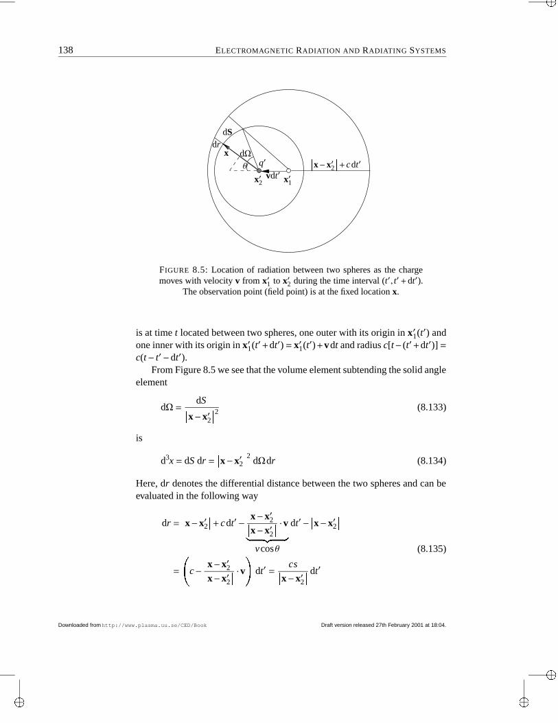
“main”2001/2/27page 138


q′

x′1x′2vdt′

x−x′2 + cdt′

dSdr

xθ

dΩ

FIGURE 8.5: Location of radiation between two spheres as the chargemoves with velocity v from x′1 to x′2 during the time interval (t′, t′ + dt′).

The observation point (field point) is at the fixed location x.

is at time t located between two spheres, one outer with its origin in x′1(t′) andone inner with its origin in x′1(t′+dt′) = x′1(t′)+vdt and radius c[t− (t′+dt′)] =

c(t− t′−dt′).From Figure 8.5 we see that the volume element subtending the solid angle

element

dΩ =dS x−x′2

2 (8.133)

is

d3x = dS dr = x−x′2

2 dΩdr (8.134)

Here, dr denotes the differential distance between the two spheres and can beevaluated in the following way

dr = x−x′2

+ cdt′− x−x′2 x−x′2 ·vM NFO P

vcosθ

dt′− x−x′2

= _ c− x−x′2 x−x′2

·v ` dt′ =cs x−x′2

dt′

(8.135)


“main”2001/2/27page 139


where Formula (8.64) on page 122 was used in the last step. Hence, the volumeelement under consideration is

d3x = dS dr =s x−x′2 dS cdt′ (8.136)

We see that the energy which is radiated per unit solid angle during the timeinterval (t′, t′ + dt′) is located in a volume element whose size is θ dependent.This explains the difference between expression (8.129) on page 136 and ex-pression (8.132) on page 137.

Let the radiated energy, integrated over Ω, be denoted Urad. After tedious,but relatively straightforward integration of Formula (8.132) on page 137, oneobtains

dUrad

dt′=µ0q′2v2

6πc1/ 1− v2

c2 0 3 (8.137)

If we know v(t′), we can integrate this expression over t′ and obtain the totalenergy radiated during the acceleration or deceleration of the particle. Thisway we obtain a classical picture of bremsstrahlung (braking radiation). Of-ten, an atomistic treatment is required for an acceptable result.

BREMSSTRAHLUNG FOR LOW SPEEDS AND SHORT ACCELERATION TIMES EXAMPLE 8.3

Calculate the bremsstrahlung when a charged particle, moving at a non-relativisticspeed, is accelerated or decelerated during an infinitely short time interval.

We approximate the velocity change at time t′ = t0 by a delta function:

v(t′) = ∆vδ(t′ − t0) (8.138)

which means that

∆v = ∞−∞ vdt (8.139)

Also, we assume v/c 1 so that, according to Formula (8.64) on page 122,

s ≈ x−x′ (8.140)

and, according to Formula (8.82) on page 127,

x−x0 ≈ x−x′ (8.141)

From the general expression (8.86) on page 128 we conclude that E ⊥ B and thatit suffices to consider E ≡ Erad . According to the “bremsstrahlung expression” forErad, Equation (8.126) on page 136,

E =q′ sinθ

4πε0c2 |x−x′|∆vδ(t′ − t0) (8.142)


“main”2001/2/27page 140


In this simple case B ≡ Brad is given by

B =Ec

(8.143)

Fourier transforming expression (8.142) on the previous page for E is trivial, yielding

Eω =q′ sinθ

8π2ε0c2 |x−x′|∆veiωt0 (8.144)

We note that the magnitude of this Fourier component is independent of ω. This is aconsequence of the infinitely short “impulsive step” δ(t′− t0) in the time domain whichproduces an infinite spectrum in the frequency domain.

The total radiation energy is given by the expression

Urad = dUrad

dt′dt′ = ∞−∞ S

E× Bµ0 ·dSdt′

=1µ0 S ∞−∞ EBdt′ d2x =

1µ0c S ∞−∞ E2 dt′ d2x

= ε0c S ∞−∞E2 dt′ d2x

(8.145)

According to Parseval’s identity [cf. Equation (7.35) on page 105] the following equal-ity holds: ∞−∞ E2 dt′ = 4π ∞0 |Eω|2 dω (8.146)

which means that the radiated energy in the frequency interval (ω,ω+ dω) is

Uradω dω = 4πε0c S

|Eω|2 d2x dω (8.147)

For our infinite spectrum, Equation (8.144) above, we obtain

Uradω dω =

q′2(∆v)2

16π3ε0c3 S

sin2 θ

|x−x′|2 d2xdω

=q′2(∆v)2

16π3ε0c3 2π

0dϕ π

0sin2 θ sinθdθdω

=q′2

3πε0c ∆v

c 2 dω2π

(8.148)

We see that the energy spectrum Uradω is independent of frequency ω. This means that

if we integrate it over all frequencies ω ∈ [0,∞], a divergent integral would result.

In reality, all spectra have finite widths, with an upper cutoff limit set by the quantum


“main”2001/2/27page 141


condition

hω =12

m(∆v)2 (8.149)

which expresses that the highest possible frequency in the spectrum is that for whichall kinetic energy difference has gone into one single field quantum (photon) withenergy hω. If we adopt the picture that the total energy is quantised in terms of Nω

photons radiated during the process, we find that

Uradω dωhω

= dNω (8.150)

or, for an electron where q′ = −|e|, where e is the elementary charge,

dNω =e2

4πε0hc2

3π ∆v

c 2 dωω≈ 1

1372

3π ∆v

c 2 dωω

(8.151)

where we used the value of the fine structure constant e2/(4πε0hc) ≈ 1/137.

Even if the number of photons becomes infinite when ω → 0, these photons havenegligible energies so that the total radiated energy is still finite.

END OF EXAMPLE 8.3 8.3.4 Cyclotron and synchrotron radiationFormula (8.86) and Formula (8.87) on page 128 for the magnetic field and theradiation part of the electric field are general, valid for any kind of motion ofthe localised charge. A very important special case is circular motion, i.e., thecase v ⊥ v.

With the charged particle orbiting in the x1x2 plane as in Figure 8.6 on thenext page, an orbit radius a, and an angular frequency ω0, we obtain

ϕ(t′) = ω0t′ (8.152a)

x′(t′) = a[x1 cosϕ(t′) + x2 sinϕ(t′)] (8.152b)

v(t′) = x′(t′) = aω0[−x1 sinϕ(t′) + x2 cosϕ(t′)] (8.152c)

v = |v| = aω0 (8.152d)

v(t′) = x′(t′) = −aω20[x1 cosϕ(t′) + x2 sinϕ(t′)] (8.152e)

v = |v| = aω20 (8.152f)

Because of the rotational symmetry we can, without loss of generality, rotateour coordinate system around the x3 axis so the relative vector x−x′ from thesource point to an arbitrary field point always lies in the x2x3 plane, i.e.,

x−x′ = x−x′

(x2 sinα+ x3 cosα) (8.153)


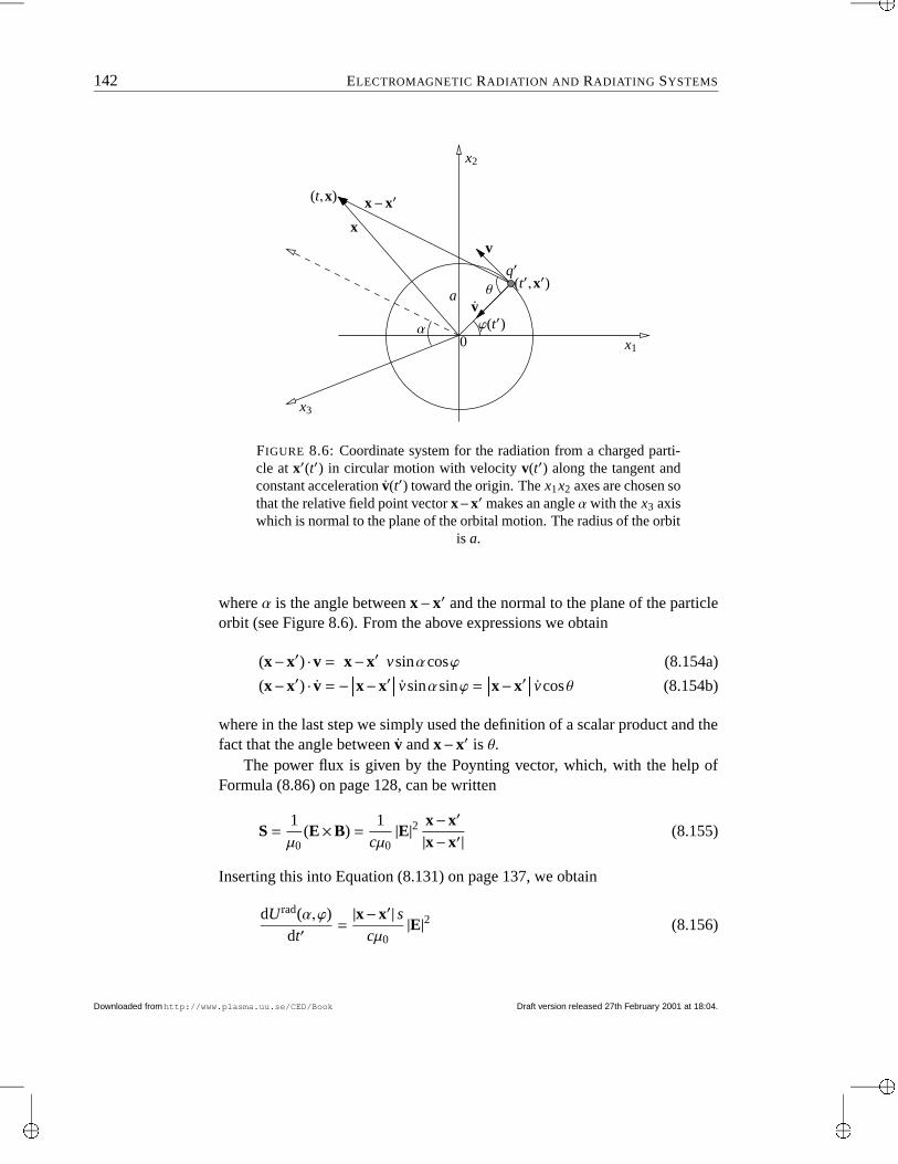
“main”2001/2/27page 142


(t′,x′)q′

θ

v

x1

x3

x2

ϕ(t′)0

α

av

(t,x) x−x′

x

FIGURE 8.6: Coordinate system for the radiation from a charged parti-cle at x′(t′) in circular motion with velocity v(t′) along the tangent andconstant acceleration v(t′) toward the origin. The x1x2 axes are chosen sothat the relative field point vector x−x′ makes an angle α with the x3 axiswhich is normal to the plane of the orbital motion. The radius of the orbit

is a.

where α is the angle between x−x′ and the normal to the plane of the particleorbit (see Figure 8.6). From the above expressions we obtain

(x−x′) ·v = x−x′

vsinαcosϕ (8.154a)

(x−x′) · v = − x−x′

vsinαsinϕ = x−x′

vcosθ (8.154b)

where in the last step we simply used the definition of a scalar product and thefact that the angle between v and x−x′ is θ.

The power flux is given by the Poynting vector, which, with the help ofFormula (8.86) on page 128, can be written

S =1µ0

(E×B) =1

cµ0|E|2 x−x′

|x−x′| (8.155)

Inserting this into Equation (8.131) on page 137, we obtain

dUrad(α,ϕ)dt′

=|x−x′| s

cµ0|E|2 (8.156)


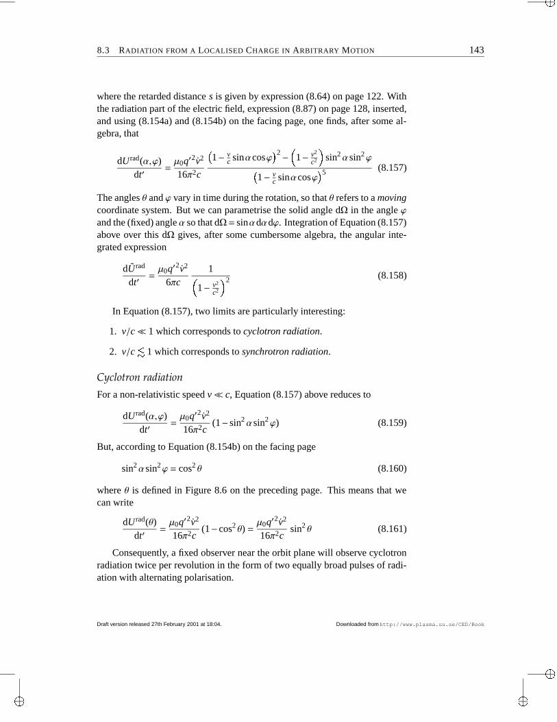
“main”2001/2/27page 143


where the retarded distance s is given by expression (8.64) on page 122. Withthe radiation part of the electric field, expression (8.87) on page 128, inserted,and using (8.154a) and (8.154b) on the facing page, one finds, after some al-gebra, that

dUrad(α,ϕ)dt′

=µ0q′2v2

16π2c4 1− v

c sinαcosϕ 5 2− / 1− v2

c2 0 sin2αsin2ϕ4 1− vc sinαcosϕ 5 5 (8.157)

The angles θ and ϕ vary in time during the rotation, so that θ refers to a movingcoordinate system. But we can parametrise the solid angle dΩ in the angle ϕand the (fixed) angle α so that dΩ = sinαdαdϕ. Integration of Equation (8.157)above over this dΩ gives, after some cumbersome algebra, the angular inte-grated expression

dUrad

dt′=µ0q′2v2

6πc1/ 1− v2

c2 0 2 (8.158)

In Equation (8.157), two limits are particularly interesting:

1. v/c 1 which corresponds to cyclotron radiation.

2. v/c v 1 which corresponds to synchrotron radiation.

Cyclotron radiationFor a non-relativistic speed v c, Equation (8.157) above reduces to

dUrad(α,ϕ)dt′

=µ0q′2v2

16π2c(1− sin2αsin2ϕ) (8.159)

But, according to Equation (8.154b) on the facing page

sin2αsin2ϕ = cos2 θ (8.160)

where θ is defined in Figure 8.6 on the preceding page. This means that wecan write

dUrad(θ)dt′

=µ0q′2v2

16π2c(1− cos2 θ) =

µ0q′2v2

16π2csin2 θ (8.161)

Consequently, a fixed observer near the orbit plane will observe cyclotronradiation twice per revolution in the form of two equally broad pulses of radi-ation with alternating polarisation.


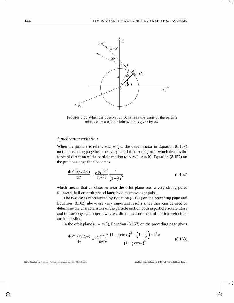
“main”2001/2/27page 144


(t′,x′)q′

v

x1

x3

x2

ϕ(t′)0

a ∆θ

∆θ

v

(t,x)x−x′

FIGURE 8.7: When the observation point is in the plane of the particleorbit, i.e., α = π/2 the lobe width is given by ∆θ.

Synchrotron radiation

When the particle is relativistic, v v c, the denominator in Equation (8.157)on the preceding page becomes very small if sinαcosϕ ≈ 1, which defines theforward direction of the particle motion (α ≈ π/2, ϕ ≈ 0). Equation (8.157) onthe previous page then becomes

dUrad(π/2,0)dt′

=µ0q′2v2

16π2c14 1− v

c5 3 (8.162)

which means that an observer near the orbit plane sees a very strong pulsefollowed, half an orbit period later, by a much weaker pulse.

The two cases represented by Equation (8.161) on the preceding page andEquation (8.162) above are very important results since they can be used todetermine the characteristics of the particle motion both in particle acceleratorsand in astrophysical objects where a direct measurement of particle velocitiesare impossible.

In the orbit plane (α = π/2), Equation (8.157) on the preceding page gives

dUrad(π/2,ϕ)dt′

=µ0q′2v2

16π2c4 1− v

c cosϕ 5 2− / 1− v2

c2 0 sin2ϕ4 1− vc cosϕ 5 5 (8.163)


“main”2001/2/27page 145


which vanishes for angles ϕ0 such that

cosϕ0 =vc

(8.164a)

sinϕ0 = 1− v2

c2 (8.164b)

Hence, the angle ϕ0 is a measure of the synchrotron radiation lobe width ∆θ;see Figure 8.7 on the preceding page. For ultra-relativistic particles, definedby

γ =1L

1− v2

c2

1, 1− v2

c2 1, (8.165)

one can approximate

ϕ0 ≈ sinϕ0 = 1− v2

c2 =1γ

(8.166)

Hence, synchrotron radiation from ultra-relativistic charges is character-ized by a radiation lobe width which is approximately

∆θ ≈ 1γ

(8.167)

This angular interval is swept by the charge during the time interval

∆t′ =∆θ

ω0(8.168)

during which the particle moves a length interval

∆l = v∆t′ = v∆θ

ω0(8.169)

in the direction toward the observer who therefore measures a pulse width oflength

∆t = ∆t′− ∆lc

= ∆t′− v∆t′

c= / 1− v

c 0 ∆t′ = / 1− vc 0 ∆θ

ω0≈ / 1− v

c 0 1γω0

= 4 1− vc5 4 1 + v

c5

1 +vcM NFO P

≈ 2

1γω0

≈ 1− v2

c2M NFO P1/γ2

12γω0

=1

2γ3

1ω0


“main”2001/2/27page 146


(8.170)

As a general rule, the spectral width of a pulse of length ∆t is ∆ω v 1/∆t.In the ultra-relativistic synchrotron case one can therefore expect frequencycomponents up to

ωmax ≈ 1∆t

= 2γ3ω0 (8.171)

A spectral analysis of the radiation pulse will exhibit Fourier components nω0

from n = 1 up to n ≈ 2γ3.When N electrons are contributing to the radiation, we can discern between

three situations:

1. All electrons are very close to each other so that the individual phasedifferences are negligible. The power will be multiplied by N2 relativeto a single electron and we talk about coherent radiation.

2. The electrons are perfectly evenly distributed in the orbit. This is thecase, for instance, for electrons in a circular current in a conductor. Inthis case the radiation fields cancel completely and no far fields are gen-erated.

3. The electrons are unevenly distributed in the orbit. This happens for anopen ring current which is subject to fluctuations of order

√N as for all

open systems. As a result we get incoherent radiation. Examples of thiscan be found both in earthly laboratories and under cosmic conditions.

Radiation in the general caseWe recall that the general expression for the radiation E field from a movingcharge concentration is given by expression (8.87) on page 128. This expres-sion in Equation (8.156) on page 142 yields the general formula

dUrad(θ)dt′

=µ0q′2 |x−x′|

16π2cs5 (x−x′)× j (x−x′)− |x−x′|vc × v 2

(8.172)

Integration over the solid angle Ω gives the totally radiated power as

dUrad

dt′=µ0q′2v2

6πc

1− v2

c2 sin2 θ/ 1− v2

c2 0 3 (8.173)

where θ is the angle between v and v.In the limit v ‖ v, sinθ= 0, which corresponds to bremsstrahlung. For v⊥ v,

sinθ = 1, which corresponds to cyclotron radiation or synchrotron radiation.


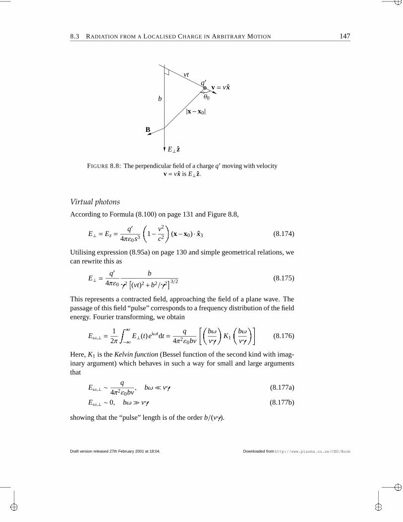
“main”2001/2/27page 147


θ0

E⊥ z

vt

b

B

v = vx

|x−x0|

q′

FIGURE 8.8: The perpendicular field of a charge q′ moving with velocityv = vx is E⊥ z.

Virtual photonsAccording to Formula (8.100) on page 131 and Figure 8.8,

E⊥ = Ez =q′

4πε0s3 1− v2

c2 (x−x0) · x3 (8.174)

Utilising expression (8.95a) on page 130 and simple geometrical relations, wecan rewrite this as

E⊥ =q′

4πε0

b

γ2 (vt)2 + b2/γ2 3/2 (8.175)

This represents a contracted field, approaching the field of a plane wave. Thepassage of this field “pulse” corresponds to a frequency distribution of the fieldenergy. Fourier transforming, we obtain

Eω,⊥ =1

2π ∞−∞ E⊥(t)eiωtdt =q

4π2ε0bvl bω

vγ K1 bωvγ (8.176)

Here, K1 is the Kelvin function (Bessel function of the second kind with imag-inary argument) which behaves in such a way for small and large argumentsthat

Eω,⊥ ∼ q4π2ε0bv

, bω vγ (8.177a)

Eω,⊥ ∼ 0, bω vγ (8.177b)

showing that the “pulse” length is of the order b/(vγ).


“main”2001/2/27page 148


Due to the equipartition of the field energy into the electric and magneticfields, the total field energy can be written

U = ε0 VE2⊥ d3x = ε0 bmax

bmin ∞−∞ E2⊥ vdt 2πbdb (8.178)

where the volume integration is over the plane perpendicular to v. With theuse of Parseval’s identity for Fourier transforms, Formula (7.35) on page 105,we can rewrite this as

U = ∞0 Uω dω = 4πε0v bmax

bmin ∞0 Eω,⊥ 2 dω2πbdb

≈ q2

2π2ε0v ∞0 vγ/ω

bmin

dbb

dω

(8.179)

from which we conclude that

Uω ≈ q2

2π2ε0vln vγ

bminω (8.180)

where an explicit value of bmin can be calculated in quantum theory only.As in the case of bremsstrahlung, it is intriguing to quantise the energy into

photons [cf. Equation (8.150) on page 141]. Then we find that

Nω dω ≈ 2απ

ln cγbminω dω

ω(8.181)

where α = e2/(4πε0hc) ≈ 1/137 is the fine structure constant.Let us consider the interaction of two electrons, 1 and 2. The result of this

interaction is that they change their linear momenta from p1 to p′1 and p2 top′2, respectively. Heisenberg’s uncertainty principle gives bmin ∼ h/

p1−p′1

so that the number of photons exchanged in the process is of the order

Nω dω ≈ 2απ

ln / cγhω

p1−p′1 0 dω

ω(8.182)

Since this change in momentum corresponds to a change in energy hω = E1 −E′1 and E1 = m0γc2, we see that

Nω dω ≈ 2απ

ln _ E1

m0c2

cp1− cp′1

E1−E′1 ` dωω

(8.183)

a formula which gives a reasonable account of electron- and photon-inducedprocesses.


“main”2001/2/27page 149


8.3.5 Radiation from charges moving in matterWhen electromagnetic radiation is propagating through matter, new phenom-ena may appear which are (at least classically) not present in vacuum. As men-tioned earlier, one can under certain simplifying assumptions include, to someextent, the influence from matter on the electromagnetic fields by introducingnew, derived field quantities D and H according to

D = ε(t,x)E = κε0E (8.184)

B = µ(t,x)H = κmµ0H (8.185)

Expressed in terms of these derived field quantities, the Maxwell equations,often called macroscopic Maxwell equations, take the form

∇ ·D = ρ(t,x) (8.186a)

∇×E +∂

∂tB = 0 (8.186b)

∇ ·B = 0 (8.186c)

∇×H− ∂

∂tD = j(t,x) (8.186d)

Assuming for simplicity that the electric permittivity ε and the magneticpermeability µ, and hence the relative permittivity κ and the relative perme-ability κm all have fixed values, independent on time and space, for each typeof material we consider, we can derive the general telegrapher’s equation [cf.Equation (2.33) on page 29]

∂2E∂ζ2 −σµ

∂E∂t−εµ∂

2E∂t2 = 0 (8.187)

describing (1D) wave propagation in a material medium.In Chapter 2 we concluded that the existence of a finite conductivity, man-

ifesting itself in a collisional interaction between the charge carriers, causesthe waves to decay exponentially with time and space. Let us therefore assumethat in our medium σ = 0 so that the wave equation simplifies to

∂2E∂ζ2 −εµ

∂2E∂t2 = 0 (8.188)

If we introduce the phase velocity in the medium as

vϕ =1√εµ

=1√

κε0κmµ0=

c√κκm

(8.189)


“main”2001/2/27page 150


where, according to Equation (1.9) on page 5, c = 1/√ε0µ0 is the speed of light,

i.e., the phase speed of electromagnetic waves in vacuum, then the generalsolution to each component of Equation (8.188) on the previous page

Ei = f (ζ − vϕt) + g(ζ + vϕt), i = 1,2,3 (8.190)

The ratio of the phase speed in vacuum and in the medium

cvϕ

=√κκm = c

√εµ

def≡ n (8.191)

is called the refractive index of the medium. In general n is a function of bothtime and space as are the quantities ε, µ, κ, and κm themselves. If, in addition,the medium is anisotropic or birefringent, all these quantities are rank-twotensor fields. Under our simplifying assumptions, in each medium we considern = Const for each frequency component of the fields.

Associated with the phase speed of a medium for a wave of a given fre-quency ω we have a wave vector, defined as

kdef≡ k k = kvϕ =

ω

vϕ

vϕvϕ

(8.192)

As in the vacuum case discussed in Chapter 2, assuming that E is time-harmonic,i.e., can be represented by a Fourier component proportional to exp−iωt, thesolution of Equation (8.188) can be written

E = E0ei(k·x−ωt) (8.193)

where now k is the wave vector in the medium given by Equation (8.192).With these definitions, the vacuum formula for the associated magnetic field,Equation (2.40) on page 30,

B =√εµ k×E =

1vϕ

k×E =1ω

k×E (8.194)

is valid also in a material medium (assuming, as mentioned, that n has a fixedconstant scalar value). A consequence of a κ 6= 1 is that the electric field will,in general, have a longitudinal component.

It is important to notice that depending on the electric and magnetic prop-erties of a medium, and, hence, on the value of the refractive index n, the phasespeed in the medium can be smaller or larger than the speed of light:

vϕ =cn

=ω

k(8.195)


“main”2001/2/27page 151


where, in the last step, we used Equation (8.192) on the facing page.If the medium has a refractive index which, as is usually the case, depen-

dent on frequency ω, we say that the medium is dispersive. Because in thiscase also k(ω) and ω(k), so that the group velocity

vg =∂ω

∂k(8.196)

has a unique value for each frequency component, and is different from vϕ.Except in regions of anomalous dispersion, vϕ is always smaller than c. Ina gas of free charges, such as a plasma, the refractive index is given by theexpression

n2(ω) = 1− ω2p

ω2 (8.197)

where

ω2p = ∑

σ

Nσq2σ

ε0mσ(8.198)

is the plasma frequency. Here mσ and Nσ denote the mass and number density,respectively, of charged particle speciesσ. In an inhomogeneous plasma, Nσ =

Nσ(x) so that the refractive index and also the phase and group velocities arespace dependent. As can be easily seen, for each given frequency, the phaseand group velocities in a plasma are different from each other. If the frequencyω is such that it coincides with ωp at some point in the medium, then at thatpoint vϕ→∞ while vg→ 0 and the wave Fourier component at ω is reflectedthere.

Vavilov-Cerenkov radiationAs we saw in Subsection 8.1, a charge in uniform, rectilinear motion in vac-uum does not give rise to any radiation; see in particular Equation (8.98a) onpage 131. Let us now consider a charge in uniform, rectilinear motion in amedium with electric properties which are different from those of a (classical)vacuum. Specifically, consider a medium where

ε = Const > ε0 (8.199a)

µ = µ0 (8.199b)

This implies that in this medium the phase speed is

vϕ =cn

=1√εµ0

< c (8.200)


“main”2001/2/27page 152


Hence, in this particular medium, the speed of propagation of (the phase planesof) electromagnetic waves is less than the speed of light in vacuum, which weknow is an absolute limit for the motion of anything, including particles. Amedium of this kind has the interesting property that particles, entering intothe medium at high speeds |v|, which, of course, are below the phase speedin vacuum, can experience that the particle speeds are higher than the phasespeed in the medium. This is the basis for the Vavilov-Cerenkov radiation thatwe shall now study.

If we recall the general derivation, in the vacuum case, of the retarded (andadvanced) potentials in Chapter 3 and the Liénard-Wiechert potentials, Equa-tions (8.63) on page 122, we realise that we obtain the latter in the mediumby a simple formal replacement c→ c/n in the expression (8.64) on page 122for s. Hence, the Liénard-Wiechert potentials in a medium characterized by arefractive index n, are

φ(t,x) =1

4πε0

q′ |x−x′| −n (x−x′)·vc

= 14πε0

q′

s(8.201a)

A(t,x) =1

4πε0c2

q′v |x−x′| −n (x−x′)·vc

= 14πε0c2

q′vs

(8.201b)

where now

s =

x−x′ −n

(x−x′) ·vc

(8.202)

The need for the absolute value of the expression for s is obvious in the casewhen v/c ≥ 1/n because then the second term can be larger than the first term;if v/c 1/n we recover the well-known vacuum case but with modified phasespeed. We also note that the retarded and advanced times in the medium are[cf. Equation (3.35) on page 43]

t′ret = t′ret(t, x−x′

) = t− k |x−x′|ω

= t− |x−x′|nc

(8.203a)

t′adv = t′adv(t, x−x′

) = t +k |x−x′|

ω= t +

|x−x′|nc

(8.203b)

so that the usual time interval t− t′ between the time measured at the point ofobservation and the retarded time in a medium becomes

t− t′ =|x−x′|n

c(8.204)


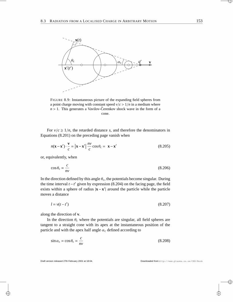
“main”2001/2/27page 153


θc αc vq′

x′(t′)

x(t)

FIGURE 8.9: Instantaneous picture of the expanding field spheres froma point charge moving with constant speed v/c > 1/n in a medium wheren > 1. This generates a Vavilov-Cerenkov shock wave in the form of a

cone.

For v/c ≥ 1/n, the retarded distance s, and therefore the denominators inEquations (8.201) on the preceding page vanish when

n(x−x′) · vc

= x−x′

nvc

cosθc = x−x′

(8.205)

or, equivalently, when

cosθc =c

nv(8.206)

In the direction defined by this angle θc, the potentials become singular. Duringthe time interval t− t′ given by expression (8.204) on the facing page, the fieldexists within a sphere of radius |x−x′| around the particle while the particlemoves a distance

l = v(t− t′) (8.207)

along the direction of v.In the direction θc where the potentials are singular, all field spheres are

tangent to a straight cone with its apex at the instantaneous position of theparticle and with the apex half angle αc defined according to

sinαc = cosθc =c

nv(8.208)


“main”2001/2/27page 154


This cone of potential singularities and field sphere circumferences propagateswith speed c/n in the form of a shock front, called Vavilov-Cerenkov radiation.1

The Vavilov-Cerenkov cone is similar in nature to the Mach cone in acoustics.In order to make some quantitative estimates of this radiation, we note that

we can describe the motion of each charged particle q′ as a current density:

j = q′vδ(x′−vt′) = q′vδ(x′− vt′)δ(y′)δ(z′)x1 (8.209)

which has the trivial Fourier transform

jω =q′

2πeiωx′/v δ(y′)δ(z′)x1 (8.210)

This Fourier component can be used in the formulae derived for a linear currentin Subsection 8.1.1 if only we make the replacements

ε0→ ε = n2ε0 (8.211a)

k→ nωc

(8.211b)

In this manner, using jω from Equation (8.210) above, the resulting Fouriertransforms of the Vavilov-Cerenkov magnetic and electric radiation fields canbe calculated from the expressions (7.11) and (7.22) on page 100, respectively.

The total energy content is then obtained from Equation (7.35) on page 105(integrated over a closed sphere at large distances). For a Fourier componentone obtains [cf. Equation (7.38) on page 105]

Uradω dΩ ≈ 1

4πε0nc

V(jω×k)e−ik·x′ d3x′

2 dΩ

=q′2nω2

16π3ε0c3

∞−∞ exp i ωx′

v− kx′ cosθ dx′

2 sin2 θdΩ

(8.212)

1The first systematic exploration of this radiation was made by P. A. Cerenkov in 1934,who was then a post-graduate student in S. I. Vavilov’s research group at the Lebedev Institutein Moscow. Vavilov wrote a manuscript with the experimental findings, put Cerenkov as theauthor, and submitted it to Nature. In the manuscript, Vavilov explained the results in terms ofradioactive particles creating Compton electrons which gave rise to the radiation (which wasthe correct interpretation), but the paper was rejected. The paper was then sent to PhysicalReview and was, after some controversy with the American editors who claimed the results tobe wrong, eventually published in 1937. In the same year, I. E. Tamm and I. M. Frank publishedthe theory for the effect (“the singing electron”). In fact, predictions of a similar effect had beenmade as early as 1888 by Heaviside, and by Sommerfeld in his 1904 paper “Radiating bodymoving with velocity of light”. On May 8, 1937, Sommerfeld sent a letter to Tamm via Austria,saying that he was surprised that his old 1904 ideas were now becoming interesting. Tamm,Frank and Cerenkov received the Nobel Prize in 1958 “for the discovery and the interpretationof the Cerenkov effect” [V. L. Ginzburg, private communication].The first observation of this type of radiation was reported by Marie Curie in 1910, but shenever pursued the exploration of it [7].


“main”2001/2/27page 155


where θ is the angle between the direction of motion, x′1, and the direction tothe observer, k. The integral in (8.212) is singular of a “Dirac delta type.” Ifwe limit the spatial extent of the motion of the particle to the closed interval[−X,X] on the x′ axis we can evaluate the integral to obtain

Uradω dΩ =

q′2nω2 sin2 θ

4π3ε0c3

sin2 4 1− nvc cosθ 5 Xω

v 4 1− nvc cosθ 5 ωv 2 dΩ (8.213)

which has a maximum in the direction θc as expected. The magnitude of thismaximum grows and its width narrows as X→∞. The integration of (8.213)over Ω therefore picks up the main contributions from θ ≈ θc. Consequently,we can set sin2 θ ≈ sin2 θc and the result of the integration is

Uradω = 2π π

0Uradω (θ) sinθdθ = dcosθ = −ξc = 2π 1

−1Uradω (ξ)dξ

≈ q′2nω2 sin2 θc

2π2ε0c3 1

−1

sin2 8 / 1 +nvξc 0 Xω

v 98 / 1 +nvξc 0 ω

v 9 2 dξ(8.214)

The integrand in (8.214) is strongly peaked near ξ = −c/(nv), or, equivalently,near cosθc = c/(nv). This means that the integrand function is practically zerooutside the integration interval ξ ∈ [−1,1]. Hence, one can extend the ξ in-tegration interval to (−∞,∞) without introducing too much an error. Via yetanother variable substitution we can therefore approximate

sin2 θc 1

−1

sin2 8 / 1 +nvξc 0 Xω

v 98 / 1 +nvξc 0 ω

v 9 2 dξ ≈ 1− c2

n2v2 cXωn ∞−∞ sin2 x

x2 dx

=cXπωn

1− c2

n2v2 (8.215)

leading to the final approximate result for the total energy loss in the frequencyinterval (ω,ω+ dω)

Uradω dω =

q′2X2πε0c2 1− c2

n2v2 ωdω (8.216)

As mentioned earlier, the refractive index is usually frequency dependent.Realising this, we find that the radiation energy per frequency unit and per unitlength is

Uradω dω2X

=q′2ω

4πε0c2 1− c2

n2(ω)v2 dω (8.217)


“main”2001/2/27page 156


This result was derived under the assumption that v/c > 1/n(ω), i.e., under thecondition that the expression inside the parentheses in the right hand side ispositive. For all media it is true that n(ω)→ 1 when ω→∞, so there exist al-ways a highest frequency for which we can obtain Vavilov-Cerenkov radiationfrom a fast charge in a medium. Our derivation above for a fixed value of n isvalid for each individual Fourier component.

Bibliography[1] R. BECKER, Electromagnetic Fields and Interactions, Dover Publications, Inc.,

New York, NY, 1982, ISBN 0-486-64290-9.

[2] M. BORN AND E. WOLF, Principles of Optics. Electromagnetic Theory of Prop-agation, Interference and Diffraction of Light, sixth ed., Pergamon Press, Ox-ford,. . . , 1980, ISBN 0-08-026481-6.

[3] V. L. GINZBURG, Applications of Electrodynamics in Theoretical Physicsand Astrophysics, Revised third ed., Gordon and Breach Science Publishers,New York, London, Paris, Montreux, Tokyo and Melbourne, 1989, ISBN 2-88124-719-9.


[5] J. B. MARION AND M. A. HEALD, Classical Electromagnetic Radiation, sec-ond ed., Academic Press, Inc. (London) Ltd., Orlando, . . . , 1980, ISBN 0-12-472257-1.


[7] J. SCHWINGER, L. L. DERAAD, JR., K. A. MILTON, AND W. TSAI, ClassicalElectrodynamics, Perseus Books, Reading, MA, 1998, ISBN 0-7382-0056-5.


[9] J. VANDERLINDE, Classical Electromagnetic Theory, John Wiley & Sons, Inc.,New York, Chichester, Brisbane, Toronto, and Singapore, 1993, ISBN 0-471-57269-1.


“main”2001/2/27page 157

FFormulae

F.1 The Electromagnetic FieldF.1.1 Maxwell’s equations

∇ ·D = ρ (F.1)

∇ ·B = 0 (F.2)

∇×E = − ∂∂t

B (F.3)

∇×H = j +∂

∂tD (F.4)

Constitutive relations

D = εE (F.5)

H =Bµ

(F.6)

j = σE (F.7)

P = ε0χE (F.8)

F.1.2 Fields and potentialsVector and scalar potentials

B = ∇×A (F.9)

E = −∇φ− ∂

∂tA (F.10)

157

“main”2001/2/27page 158

158 FORMULAE

Lorentz’ gauge condition in vacuum

∇ ·A +1c2

∂

∂tφ = 0 (F.11)

F.1.3 Force and energyPoynting’s vector

S = E×H (F.12)

Maxwell’s stress tensor

Ti j = EiD j + HiB j− 12δi j (EkDk + HkBk) (F.13)

F.2 Electromagnetic RadiationF.2.1 Relationship between the field vectors in a plane

wave

B =k×E

c(F.14)

F.2.2 The far fields from an extended source distribution

Bradω (x) =

−iµ0

4πeik|x|

|x| V′d3x′ e−ik·x′ jω×k (F.15)

Eradω (x) =

i4πε0c

eik|x|

|x| x× V′d3x′ e−ik·x′ jω×k (F.16)

F.2.3 The far fields from an electric dipole

Bradω (x) = −ωµ0

4πeik|x|

|x| pω×k (F.17)

Eradω (x) = − 1

4πε0

eik|x|

|x| (pω×k)×k (F.18)


“main”2001/2/27page 159

F.3 SPECIAL RELATIVITY 159

F.2.4 The far fields from a magnetic dipole

Bradω (x) = −µ0

4πeik|x|

|x| (mω×k)×k (F.19)

Eradω (x) =

k4πε0c

eik|x|

|x| mω×k (F.20)

F.2.5 The far fields from an electric quadrupole

Bradω (x) =

iµ0ω

8πeik|x|

|x| 4 k ·Qω5 ×k (F.21)

Eradω (x) =

i8πε0

eik|x|

|x| 4 k ·Qω5 ×k ×k (F.22)

F.2.6 The fields from a point charge in arbitrary motion

E(t,x) =q

4πε0s3 (x−x0) 1− v2

c2 + (x−x′)× (x−x0)× vc2 (F.23)

B(t,x) = (x−x′)× E(t,x)c|x−x′| (F.24)

s = x−x′

− (x−x′) · vc

(F.25)

x−x0 = (x−x′)− |x−x′|vc

(F.26) ∂t′

∂t x=|x−x′|

s(F.27)

F.2.7 The fields from a point charge in uniform motion

E(t,x) =q

4πε0 s3 (x−x0) 1− v2

c2 (F.28)

B(t,x) =v×E(t,x)

c2 (F.29)

s = |x−x0|2− (x−x0)×vc 2

(F.30)


“main”2001/2/27page 160

160 FORMULAE

F.3 Special RelativityF.3.1 Metric tensor

gµν = ABBC 1 0 0 00 −1 0 00 0 −1 00 0 0 −1

DFEEG (F.31)

F.3.2 Covariant and contravariant four-vectorsvµ = gµνv

ν (F.32)

F.3.3 Lorentz transformation of a four-vector

x′µ = Λµνxν (F.33)

Λµν = ABBC γ −γβ 0 0

−γβ γ 0 00 0 1 00 0 0 1

DFEEG (F.34)

γ =1;

1−β2(F.35)

β =vc

(F.36)

F.3.4 Invariant line element

ds = cdtγ

= cdτ (F.37)

F.3.5 Four-velocity

uµ =dxdτ

µ

= γ(c,v) (F.38)

F.3.6 Four-momentum

pµ = m0cuµ = Ec, p (F.39)


“main”2001/2/27page 161

F.4 VECTOR RELATIONS 161

F.3.7 Four-current densityjµ = ρ0uµ (F.40)

F.3.8 Four-potential

Aµ = φc, A (F.41)

F.3.9 Field tensor

Fµν = ∂µAν−∂νAµ = ABBC 0 −Ex/c −Ey/c −Ez/cEx/c 0 −Bz By

Ey/c Bz 0 −Bx

Ez/c By Bx 0

DFEEG (F.42)

F.4 Vector RelationsLet x be the radius vector (coordinate vector) from the origin to the point(x1, x2, x3) ≡ (x,y,z) and let |x| denote the magnitude (“length”) of x. Let fur-ther α(x),β(x), . . . be arbitrary scalar fields and a(x),b(x),c(x),d(x), . . . arbi-trary vector fields.

The differential vector operator ∇ is in Cartesian coordinates given by

∇ ≡3

∑i=1

xi∂

∂xi

def≡ xi∂

∂xi

def≡ ∂ (F.43)

where xi, i = 1,2,3 is the ith unit vector and x1 ≡ x, x2 ≡ y, and x3 ≡ z. Incomponent (tensor) notation ∇ can be written

∇i = ∂i = ∂

∂x1,∂

∂x2,∂

∂x3 = ∂∂x,∂

∂y,∂

∂z (F.44)

F.4.1 Spherical polar coordinatesBase vectors

r = sinθcosϕx1 + sinθ sinϕx2 + cosθx3 (F.45a)

θ = cosθcosϕx1 + cosθ sinϕx2− sinθx3 (F.45b)

ϕ = −sinϕx1 + cosϕx2 (F.45c)


“main”2001/2/27page 162

162 FORMULAE

x1 = sinθcosϕr + cosθcosϕθ− sinϕϕ (F.46a)

x2 = sinθ sinϕr + cosθ sinϕθ+ cosϕϕ (F.46b)

x3 = cosθ r− sinθθ (F.46c)

Directed line element

dx x = dl = dr r + r dθ θ+ r2 sinθdϕ ϕ (F.47)

Solid angle element

dΩ = sinθdθdϕ (F.48)

Directed area element

d2x n = dS = dS r = r2dΩ r (F.49)

Volume element

d3x = dV = drdS = r2dr dΩ (F.50)

F.4.2 Vector formulae

General vector algebraic identities

a ·b = b ·a = δi jaib j = abcosθ (F.51)

a×b = −b×a = εi jka jbk xi (F.52)

a · (b× c) = (a×b) · c (F.53)

a× (b× c) = b(a · c)− c(a ·b) (F.54)

a× (b× c) + b× (c×a) + c× (a×b) = 0 (F.55)

(a×b) · (c×d) = a · [b× (c×d)] = (a · c)(b ·d)− (a ·d)(b · c) (F.56)

(a×b)× (c×d) = (a×b ·d)c− (a×b · c)d (F.57)


“main”2001/2/27page 163

F.4 VECTOR RELATIONS 163

General vector analytic identities

∇(αβ) = α∇β+β∇α (F.58)

∇ · (αa) = a ·∇α+α∇ ·a (F.59)

∇× (αa) = α∇×a−a×∇α (F.60)

∇ · (a×b) = b · (∇×a)−a · (∇×b) (F.61)

∇× (a×b) = a(∇ ·b)−b(∇ ·a) + (b ·∇)a− (a ·∇)b (F.62)

∇(a ·b) = a× (∇×b) + b× (∇×a) + (b ·∇)a + (a ·∇)b (F.63)

∇ ·∇α = ∇2α (F.64)

∇×∇α = 0 (F.65)

∇ · (∇×a) = 0 (F.66)

∇× (∇×a) = ∇(∇ ·a)−∇2a (F.67)

Special identities

In the following k is an arbitrary constant vector.

∇ ·x = 3 (F.68)

∇×x = 0 (F.69)

∇|x| = x|x| (F.70)

∇ 1|x| = − x

|x|3 (F.71)

∇ · x|x|3 = −∇2 1

|x| = 4πδ(x) (F.72)

∇ k|x| = k · ∇ 1

|x| = −k ·x|x|3 (F.73)

∇× k× x|x|3 = −∇ k ·x

|x|3 if |x| 6= 0 (F.74)

∇2 k|x| = k∇2 1

|x| = −4πkδ(x) (F.75)

∇× (k×a) = k(∇ ·a) + k× (∇×a)−∇(k ·a) (F.76)

Integral relations

Let V(S ) be the volume bounded by the closed surface S (V). Denote the 3-dimensional volume element by d3x(≡ dV) and the surface element, directed


“main”2001/2/27page 164

164 FORMULAE

along the outward pointing surface normal unit vector n, by dS(≡ d2x n). Then V(∇ ·a)d3x = S

dS ·a (F.77) V(∇α)d3x = S

dSα (F.78) V(∇×a)d3x = S

dS×a (F.79)

If S (C) is an open surface bounded by the contour C(S ), whose line ele-ment is dl, then C

αdl = SdS×∇α (F.80) C

a ·dl = SdS · (∇×a) (F.81)

Bibliography[1] G. B. ARFKEN AND H. J. WEBER, Mathematical Methods for Physicists, fourth,

international ed., Academic Press, Inc., San Diego, CA . . . , 1995, ISBN 0-12-059816-7.

[2] P. M. MORSE AND H. FESHBACH, Methods of Theoretical Physics, Part I.McGraw-Hill Book Company, Inc., New York, NY . . . , 1953, ISBN 07-043316-8.



“main”2001/2/27page 165

MMathematical

Methods

M.1 Scalars, Vectors and TensorsEvery physical observable can be described by a geometric object. We willdescribe the observables in classical electrodynamics mathematically in termsof scalars, pseudoscalars, vectors, pseudovectors, tensors or pseudotensors andwill not exploit differential forms to any significant degree.

A scalar describes a scalar quantity which may or may not be constant intime and/or space. A vector describes some kind of physical motion due tovection and a tensor describes the motion or deformation due to some form oftension. However, generalisations to more abstract notions of these quantitiesare commonplace. The difference between a scalar, vector and tensor and apseudoscalar, pseudovector and a pseudotensor is that the latter behave differ-ently under such coordinate transformations which cannot be reduced to purerotations.

Throughout we adopt the convention that Latin indices i, j,k, l, . . . run overthe range 1,2,3 to denote vector or tensor components in the real Euclideanthree-dimensional (3D) configuration space 3 , and Greek indices µ,ν,κ,λ, . . . ,which are used in four-dimensional (4D) space, run over the range 0,1,2,3.

M.1.1 VectorsRadius vector

Any vector can be represented mathematically in several different ways. Onesuitable representation is in terms of an ordered N-tuple, or row vector, of thecoordinates xN where N is the dimensionality of the space under consideration.The most basic vector is radius vector which is the vector from the origin to thepoint of interest. Its N-tuple representation simply enumerates the coordinateswhich describe this point. In this sense, the radius vector from the origin to apoint is synonymous with the coordinates of the point itself.

165

“main”2001/2/27page 166

166 MATHEMATICAL METHODS

In the 3D space 3 , we have N = 3 and the radius vector can be representedby the triplet (x1, x2, x3) of coordinates xi, i = 1,2,3. The coordinates xi arescalar quantities which describe the position along the unit base vectors xi

which span 3 . Therefore a representation of the radius vector in 3 is

x =3

∑i=1

xixidef≡ xixi (M.1)

where we have introduced Einstein’s summation convention (EΣ) which statesthat a repeated index in a term implies summation over the range of the index inquestion. Whenever possible and convenient we shall in the following alwaysassume EΣ and suppress explicit summation in our formulae. Typographically,we represent a 3D vector by a boldface letter or symbol in a Roman font.

Alternatively, we may describe the radius vector in component notation asfollows:

xidef≡ (x1, x2, x3) ≡ (x,y,z) (M.2)

This component notation is particularly useful in 4D space where we canrepresent the radius vector either in its contravariant component form

xµdef≡ (x0, x1, x2, x3) (M.3)

or its covariant component form

xµdef≡ (x0, x1, x2, x3) (M.4)

The relation between the covariant and contravariant forms is determined bythe metric tensor (also known as the fundamental tensor) whose actual form isdictated by the physics. The dual representation of vectors in contravariant andcovariant forms is most convenient when we work in a non-Euclidean vectorspace with an indefinite metric. An example is Lorentz space < 4 which is a4D Riemannian space. < 4 is often utilised to formulate the special theory ofrelativity.

We note that for a change of coordinates xµ→ x′µ = x′µ(x0, x1, x2, x3), dueto a transformation from a system Σ to another system Σ′, the differential radiusvector dxµ transforms as

dx′µ =∂x′µ

∂xνdxν (M.5)

which follows trivially from the rules of differentiation of x′µ considered asfunctions of four variables xν.


“main”2001/2/27page 167

M.1 SCALARS, VECTORS AND TENSORS 167

M.1.2 FieldsA field is a physical entity which depends on one or more continuous parame-ters. Such a parameter can be viewed as a “continuous index” which enumer-ates the “coordinates” of the field. In particular, in a field which depends onthe usual radius vector x of 3 , each point in this space can be considered asone degree of freedom so that a field is a representation of a physical entitywhich has an infinite number of degrees of freedom.

Scalar fields

We denote an arbitrary scalar field in 3 by

α(x) = α(x1, x2, x3)def≡ α(xi) (M.6)

This field describes how the scalar quantity α varies continuously in 3D 3

space.In 4D, a four-scalar field is denoted

α(x0, x1, x2, x3)def≡ α(xµ) (M.7)

which indicates that the four-scalar α depends on all four coordinates spanningthis space. Since a four-scalar has the same value at a given point regardlessof coordinate system, it is also called an invariant.

Analogous to the transformation rule, Equation (M.5) on the precedingpage, for the differential dxµ, the transformation rule for the differential oper-ator ∂/∂xµ under a transformation xµ→ x′µ becomes

∂

∂x′µ=∂xν

∂x′µ∂

∂xν(M.8)

which, again, follows trivially from the rules of differentiation.

Vector fields

We can represent an arbitrary vector field a(x) in 3 as follows:

a(x) = xiai(x) (M.9)

In component notation this same vector can be represented as

ai(x) = (a1(x),a2(x),a3(x)) = ai(x j) (M.10)


“main”2001/2/27page 168


In 4D, an arbitrary four-vector field in contravariant component form canbe represented as

aµ(xν) = (a0(xν),a1(xν),a2(xν),a3(xν)) (M.11)

or, in covariant component form, as

aµ(xν) = (a0(xν),a1(xν),a2(xν),a3(xν)) (M.12)

where xν is the radius four-vector. Again, the relation between aµ and aµ isdetermined by the metric of the physical 4D system under consideration.

Whether an arbitrary N-tuple fulfils the requirement of being an (N-dimen-sional) contravariant vector or not, depends on its transformation propertiesduring a change of coordinates. For instance, in 4D an assemblage yµ =

(y0,y1,y2,y3) constitutes a contravariant four-vector (or the contravariant com-ponents of a four-vector) if and only if, during a transformation from a systemΣ with coordinates xµ to a system Σ′ with coordinates x′µ, it transforms to thenew system according to the rule

y′µ =∂x′µ

∂xνyν (M.13)

i.e., in the same way as the differential coordinate element dxµ transformsaccording to Equation (M.5) on page 166.

The analogous requirement for a covariant four-vector is that it transforms,during the change from Σ to Σ′, according to the rule

y′µ =∂xν

∂x′µyν (M.14)

i.e., in the same way as the differential operator ∂/∂xµ transforms according toEquation (M.8) on the previous page.

Tensor fieldsWe denote an arbitrary tensor field in 3 by A(x). This tensor field can berepresented in a number of ways, for instance in the following matrix form:

A(x) = AC A11(x) A12(x) A13(x)A21(x) A22(x) A23(x)A31(x) A32(x) A33(x)

DG def≡ 4 Ai j(xk) 5 (M.15)

where, in the last member, we have again used the more compact componentnotation. Strictly speaking, the tensor field described here is a tensor of ranktwo.


“main”2001/2/27page 169


A particularly simple rank-two tensor in 3 is the 3D Kronecker delta sym-bol δi j, with the following properties:

δi j = H 0 if i 6= j

1 if i = j(M.16)

The 3D Kronecker delta has the following matrix representation

(δi j) = AC 1 0 00 1 00 0 1

DG (M.17)

Another common and useful tensor is the fully antisymmetric tensor ofrank 3, also known as the Levi-Civita tensor

εi jk = =>? >@ 1 if i, j,k is an even permutation of 1,2,3

0 if at least two of i, j,k are equal

−1 if i, j,k is an odd permutation of 1,2,3

(M.18)

with the following further property

εi jkεilm = δ jlδkm−δ jmδkl (M.19)

In fact, tensors may have any rank n. In this picture a scalar is consideredto be a tensor of rank n = 0 and a vector a tensor of rank n = 1. Consequently,the notation where a vector (tensor) is represented in its component form iscalled the tensor notation. A tensor of rank n = 2 may be represented by a two-dimensional array or matrix whereas higher rank tensors are best representedin their component forms (tensor notation).

In 4D, we have three forms of four-tensor fields of rank n. We speak of

• a contravariant four-tensor field, denoted Aµ1µ2...µn(xν),

• a covariant four-tensor field, denoted Aµ1µ2...µn(xν),

• a mixed four-tensor field, denoted Aµ1µ2...µkµk+1...µn (xν).

The 4D metric tensor (fundamental tensor) mentioned above is a particu-larly important four-tensor of rank 2. In covariant component form we shalldenote it gµν. This metric tensor determines the relation between an arbitrarycontravariant four-vector aµ and its covariant counterpart aµ according to thefollowing rule:

aµ(xκ)def≡ gµνa

ν(xκ) (M.20)


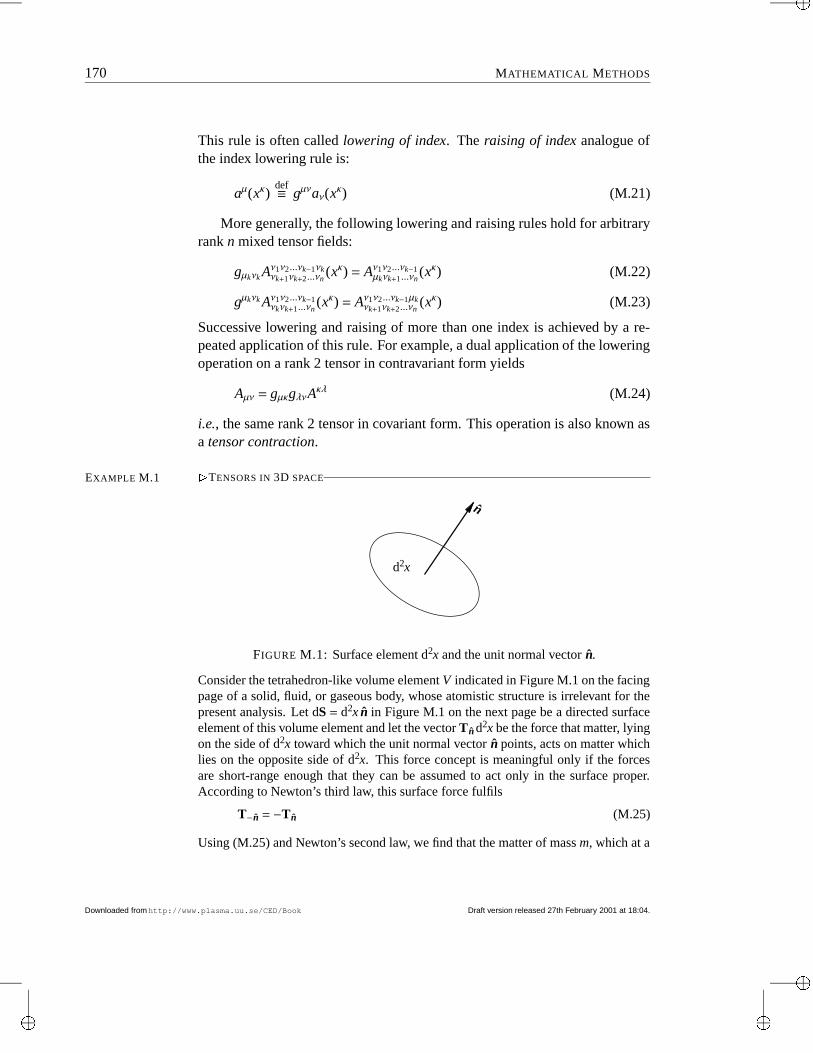
“main”2001/2/27page 170


This rule is often called lowering of index. The raising of index analogue ofthe index lowering rule is:

aµ(xκ)def≡ gµνaν(xκ) (M.21)

More generally, the following lowering and raising rules hold for arbitraryrank n mixed tensor fields:

gµkνk Aν1ν2...νk−1νkνk+1νk+2...νn

(xκ) = Aν1ν2...νk−1µkνk+1...νn

(xκ) (M.22)

gµkνk Aν1ν2...νk−1νkνk+1...νn

(xκ) = Aν1ν2...νk−1µkνk+1νk+2...νn

(xκ) (M.23)

Successive lowering and raising of more than one index is achieved by a re-peated application of this rule. For example, a dual application of the loweringoperation on a rank 2 tensor in contravariant form yields

Aµν = gµκgλνAκλ (M.24)

i.e., the same rank 2 tensor in covariant form. This operation is also known asa tensor contraction.

TENSORS IN 3D SPACEEXAMPLE M.1

n

d2x

FIGURE M.1: Surface element d2x and the unit normal vector n.

Consider the tetrahedron-like volume element V indicated in Figure M.1 on the facingpage of a solid, fluid, or gaseous body, whose atomistic structure is irrelevant for thepresent analysis. Let dS = d2x n in Figure M.1 on the next page be a directed surfaceelement of this volume element and let the vector Tn d2x be the force that matter, lyingon the side of d2x toward which the unit normal vector n points, acts on matter whichlies on the opposite side of d2x. This force concept is meaningful only if the forcesare short-range enough that they can be assumed to act only in the surface proper.According to Newton’s third law, this surface force fulfils

T−n = −Tn (M.25)

Using (M.25) and Newton’s second law, we find that the matter of mass m, which at a


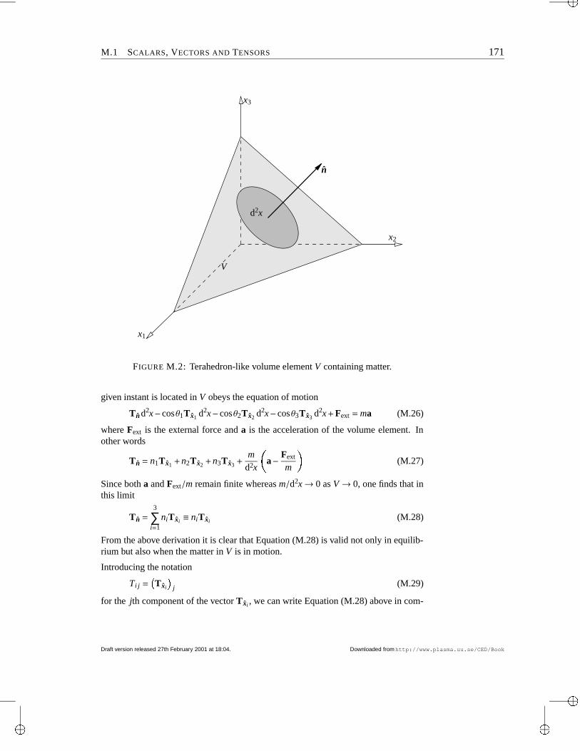
“main”2001/2/27page 171


x1

V

d2x

n

x3

x2

FIGURE M.2: Terahedron-like volume element V containing matter.

given instant is located in V obeys the equation of motion

Tn d2x− cosθ1Tx1 d2x− cosθ2Tx2 d2x− cosθ3Tx3 d2x + Fext = ma (M.26)

where Fext is the external force and a is the acceleration of the volume element. Inother words

Tn = n1Tx1 + n2Tx2 + n3Tx3 +m

d2x a− Fext

m (M.27)

Since both a and Fext/m remain finite whereas m/d2x→ 0 as V → 0, one finds that inthis limit

Tn =3

∑i=1

niTxi ≡ niTxi (M.28)

From the above derivation it is clear that Equation (M.28) is valid not only in equilib-rium but also when the matter in V is in motion.

Introducing the notation

Ti j = Txi j (M.29)

for the jth component of the vector Txi , we can write Equation (M.28) above in com-


“main”2001/2/27page 172


ponent form as follows

T n j = (Tn) j =3

∑i=1

niTi j ≡ niTi j (M.30)

Using Equation (M.30), we find that the component of the vector T n in the directionof an arbitrary unit vector m is

T nm = Tn · m

=3

∑j=1

T n jm j =3

∑j=1

t3

∑i=1

niTi j u m j ≡ niTi jm j = n ·T · m (M.31)

Hence, the jth component of the vector T xi , here denoted Ti j, can be interpreted as thei jth component of a tensor T. Note that T nm is independent of the particular coordinatesystem used in the derivation.

We shall now show how one can use the momentum law (force equation) to derivethe equation of motion for an arbitrary element of mass in the body. To this end weconsider a part V of the body. If the external force density (force per unit volume) isdenoted by f and the velocity for a mass element dm is denoted by v, we obtain

ddt V

vdm = Vfd3x + S

Tn d2x (M.32)

The jth component of this equation can be written V

ddt

v j dm = Vf j d3x + S

T n j d2x = Vf j d3x + S

niTi j d2x (M.33)

where, in the last step, Equation (M.30) above was used. Setting dm = ρd3x and usingthe divergence theorem on the last term, we can rewrite the result as V

ρddt

v j d3x = Vf j d3x + V

∂Ti j

∂xid3x (M.34)

Since this formula is valid for any arbitrary volume, we must require that

ρddt

v j− f j − ∂Ti j

∂xi= 0 (M.35)

or, equivalently

ρ∂v j

∂t+ρv ·∇v j − f j − ∂Ti j

∂xi= 0 (M.36)

Note that ∂v j/∂t is the rate of change with time of the velocity component v j at a fixedpoint x = (x1, x1, x3).

END OF EXAMPLE M.1 Downloaded fromhttp://www.plasma.uu.se/CED/Book Draft version released 27th February 2001 at 18:04.

“main”2001/2/27page 173


M.1.3 Vector algebraScalar product

The scalar product (dot product, inner product) of two arbitrary 3D vectors aand b in ordinary 3 space is the scalar number

a ·b = xiai · x jb j = xi · x jaib j = δi jaib j = aibi (M.37)

where we used the fact that the scalar product xi · x j is a representation ofthe Kronecker delta δi j defined in Equation (M.16) on page 169. In Russianliterature, the scalar product is often denoted (ab).

In 4D space we define the scalar product of two arbitrary four-vectors aµ

and bµ in the following way

aµbµ = gνµaνbµ = aνbν = gµνaµbν (M.38)

where we made use of the index lowering and raising rules (M.20) and (M.21).The result is a four-scalar, i.e., an invariant which is independent on in whichinertial system it is measured.

The quadratic differential form

ds2 = gµνdxνdxµ = dxµdxµ (M.39)

i.e., the scalar product of the differential radius four-vector with itself, is aninvariant called the metric. It is also the square of the line element ds which isthe distance between neighbouring points with coordinates xµ and xµ+ dxµ.

INNER PRODUCTS IN COMPLEX VECTOR SPACE EXAMPLE M.2

A 3D complex vector A is a vector in 3 (or, if we like, in 6 ), expressed in terms oftwo real vectors aR and aI in 3 in the following way

Adef≡ aR + iaI = aR aR + iaI aI

def≡ A A ∈ 3 (M.40)

The inner product of A with itself may be defined as

A2 def≡ A ·A = a2R−a2

I + 2iaR ·aIdef≡ A2 ∈ (M.41)

from which we find that

A = w a2R−a2

I + 2iaR ·aI ∈ (M.42)

Using this in Equation (M.40) above, we see that we can interpret this so that the


“main”2001/2/27page 174


complex unit vector is

A =AA

=aRw a2

R−a2I + 2iaR ·aI

aR + iaIw a2

R−a2I + 2iaR ·aI

aI

=aR w a2

R−a2I −2iaR ·aI

a2R + a2

I

aR + iaI w a2

R −a2I −2iaR ·aI

a2R + a2

I

aI ∈ 3

(M.43)

On the other hand, the definition of the scalar product in terms of the inner product ofcomplex vector with its own complex conjugate yields

|A|2 def≡ A ·A∗ = a2R + a2

I = |A|2 (M.44)

with the help of which we can define the unit vector as

A =A|A| =

aRw a2R + a2

I

aR + iaIw a2R + a2

I

aI

=aR w a2

R + a2I

a2R + a2

I

aR + iaI w a2

R + a2I

a2R + a2

I

aI ∈ 3

(M.45)

END OF EXAMPLE M.2 SCALAR PRODUCT, NORM AND METRIC IN LORENTZ SPACEEXAMPLE M.3

In x 4 the metric tensor attains a simple form [see Equation (4.10) on page 51 for anexample] and, hence, the scalar product in Equation (M.38) on the previous page canbe evaluated almost trivially and becomes

aµbµ = (a0,−a) · (b0,b) = a0b0 −a ·b (M.46)

The important scalar product of the x 4 radius four-vector with itself becomes

xµxµ = (x0,−x) · (x0,x) = (ct,−x) · (ct,x)

= (ct)2 − (x1)2 − (x2)2 − (x3)2 = s2(M.47)

which is the indefinite, real norm of x 4 . The x 4 metric is the quadratic differentialform

ds2 = dxµdxµ = c2(dt)2 − (dx1)2 − (dx2)2 − (dx3)2 (M.48)


“main”2001/2/27page 175


METRIC IN GENERAL RELATIVITY EXAMPLE M.4

In the general theory of relativity, several important problems are treated in a 4Dspherical polar coordinate system. Then the radius four-vector can be given asxµ = (ct,r, θ,φ) and the metric tensor is

gµν = !##$ eκ 0 0 00 e−λ 0 00 0 −r2 00 0 0 −r2 sin2 θ

' ))+ (M.49)

where κ = κ(ct,r, θ,φ) and λ = λ(ct,r, θ,φ). In such a space, the metric takes the form

ds2 = c2eκ(dt)2 − eλ(dr)2− r2(dθ)2 − r2 sin2 θ(dφ)2 (M.50)

In general relativity the metric tensor is not given a priori but is determined by theEinstein equations.

END OF EXAMPLE M.4 Dyadic productThe dyadic product field A(x) ≡ a(x)b(x) with two juxtaposed vector fieldsa(x) and b(x) is the outer product of a and b. Operating on this dyad from theright and from the left with an inner product of an vector c one obtains

A · c def≡ ab · c def≡ a(b · c) (M.51a)

c ·A def≡ c ·abdef≡ (c ·a)b (M.51b)

i.e., new vectors, proportional to a and b, respectively. In mathematics, adyadic product is often called tensor product and is frequently denoted a⊗b.

In matrix notation the outer product of a and b is written

ab = 4 x1 x2 x35 AC a1b1 a1b2 a1b3

a1b2 a2b2 a2b3

a1b3 a3b2 a3b3

DG AC x1

x2

x3

DG (M.52)

which means that we can represent the tensor A(x) in matrix form as

4 Ai j(xk) 5 = AC a1b1 a1b2 a1b3

a1b2 a2b2 a2b3

a1b3 a3b2 a3b3

DG (M.53)

which we identify with expression (M.15) on page 168, viz. a tensor in matrixnotation.


“main”2001/2/27page 176


Vector productThe vector product or cross product of two arbitrary 3D vectors a and b inordinary 3 space is the vector

c = a×b = εi jka jbk xi (M.54)

Here εi jk is the Levi-Civita tensor defined in Equation (M.18) on page 169.Sometimes the vector product of a and b is denoted a∧b or, particularly in theRussian literature, [ab].

A spatial reversal of the coordinate system (x′1, x′2, x′3) = (−x1,−x2,−x3)

changes sign of the components of the vectors a and b so that in the new co-ordinate system a′ = −a and b′ = −b, which is to say that the direction of anordinary vector is not dependent on the choice of directions of the coordinateaxes. On the other hand, as is seen from Equation (M.54), the cross productvector c does not change sign. Therefore a (or b) is an example of a “true”vector, or polar vector, whereas c is an example of an axial vector, or pseu-dovector.

A prototype for a pseudovector is the angular momentum vector and hencethe attribute “axial.” Pseudovectors transform as ordinary vectors under trans-lations and proper rotations, but reverse their sign relative to ordinary vectorsfor any coordinate change involving reflection. Tensors (of any rank) whichtransform analogously to pseudovectors are called pseudotensors. Scalars aretensors of rank zero, and zero-rank pseudotensors are therefore also calledpseudoscalars, an example being the pseudoscalar xi · (x j × xk). This tripleproduct is a representation of the i jk component of the Levi-Civita tensor εi jk

which is a rank three pseudotensor.

M.1.4 Vector analysisThe del operatorIn 3 the del operator is a differential vector operator, denoted in Gibbs’notation by ∇ and defined as

∇ def≡ xi∂

∂xi

def≡ ∂ (M.55)

where xi is the ith unit vector in a Cartesian coordinate system. Since theoperator in itself has vectorial properties, we denote it with a boldface nabla.In “component” notation we can write

∂i = ∂

∂x1,∂

∂x2,∂

∂x3 (M.56)


“main”2001/2/27page 177


In 4D, the contravariant component representation of the four-del operatoris defined by

∂µ = ∂

∂x0,∂

∂x1,∂

∂x2,∂

∂x3 (M.57)

whereas the covariant four-del operator is

∂µ = ∂

∂x0 ,∂

∂x1 ,∂

∂x2 ,∂

∂x3 (M.58)

We can use this four-del operator to express the transformation properties(M.13) and (M.14) on page 168 as

y′µ = 4 ∂νx′µ 5 yν (M.59)

and

y′µ = 4 ∂′µxν 5 yν (M.60)

respectively.THE FOUR-DEL OPERATOR IN LORENTZ SPACE EXAMPLE M.5

In x 4 the contravariant form of the four-del operator can be represented as

∂µ = 1c∂

∂t,−∂ = 1

c∂

∂t,−∇ (M.61)

and the covariant form as

∂µ = 1c∂

∂t,∂ = 1

c∂

∂t,∇ (M.62)

Taking the scalar product of these two, one obtains

∂µ∂µ =1c2

∂2

∂t2 −∇2 =q 2 (M.63)

which is the d’Alembert operator, sometimes denotedq

, and sometimes defined withan opposite sign convention.

END OF EXAMPLE M.5 Draft version released 27th February 2001 at 18:04. Downloaded fromhttp://www.plasma.uu.se/CED/Book

“main”2001/2/27page 178


With the help of the del operator we can define the gradient, divergenceand curl of a tensor (in the generalised sense).

The gradient

The gradient of an 3 scalar field α(x), denoted ∇α(x), is an 3 vector fielda(x):

∇α(x) = ∂α(x) = xi∂iα(x) = a(x) (M.64)

From this we see that the boldface notation for the nabla and del operators isvery handy as it elucidates the 3D vectorial property of the gradient.

In 4D, the four-gradient is a covariant vector, formed as a derivative of afour-scalar field α(xµ), with the following component form:

∂µα(xν) =∂α(xν)∂xµ

(M.65)

GRADIENTS OF SCALAR FUNCTIONS OF RELATIVE DISTANCES IN 3DEXAMPLE M.6

Very often electrodynamic quantities are dependent on the relative distance in 3 be-tween two vectors x and x′, i.e., on |x− x′|. In analogy with Equation (M.55) onpage 176, we can define the “primed” del operator in the following way:

∇′ = xi∂

∂x′i= ∂′ (M.66)

Using this, the “unprimed” version, Equation (M.55) on page 176, and elementaryrules of differentiation, we obtain the following two very useful results:

∇ |x−x′| = xi∂|x−x′|∂xi

=x−x′

|x−x′| = −xi∂|x−x′|∂x′i

= −∇′ |x−x′| (M.67)

and

∇ 1|x−x′| = − x−x′

|x−x′|3 = −∇′ 1|x−x′| (M.68)


“main”2001/2/27page 179


The divergence

We define the 3D divergence of a vector field in 3 as

∇ ·a(x) = ∂ · x ja j(x) = δi j∂ia j(x) = ∂iai(x) =∂ai(x)∂xi

= α(x) (M.69)

which, as indicated by the notation α(x), is a scalar field in 3 . We may thinkof the divergence as a scalar product between a vectorial operator and a vector.As is the case for any scalar product, the result of a divergence operation is ascalar. Again we see that the boldface notation for the 3D del operator is veryconvenient.

The four-divergence of a four-vector aµ is the following four-scalar:

∂µaµ(xν) = ∂µaµ(xν) =∂aµ(xν)∂xµ

(M.70)

DIVERGENCE IN 3D EXAMPLE M.7

For an arbitrary 3 vector field a(x′), the following relation holds:

∇′ · a(x′)|x−x′| =

∇′ ·a(x′)|x−x′| + a(x′) ·∇′ 1

|x−x′| (M.71)

which demonstrates how the “primed” divergence, defined in terms of the “primed”del operator in Equation (M.66) on the facing page, works.

END OF EXAMPLE M.7 The Laplacian

The 3D Laplace operator or Laplacian can be described as the divergence ofthe gradient operator:

∇2 = ∆ = ∇ ·∇ =∂

∂xixi · x j

∂

∂x j= δi j∂i∂ j = ∂2

i =∂2

∂x2i

≡3

∑i=1

∂2

∂x2i

(M.72)

The symbol ∇2 is sometimes read del squared. If, for a scalar field α(x),∇2α < 0 at some point in 3D space, it is a sign of concentration of α at thatpoint.


“main”2001/2/27page 180


THE LAPLACIAN AND THE DIRAC DELTAEXAMPLE M.8

A very useful formula in 3D 3 is

∇ ·∇ 1|x−x′| = ∇2 1

|x−x′| = −4πδ(x−x′) (M.73)

where δ(x−x′) is the 3D Dirac delta “function.”

END OF EXAMPLE M.8 The curlIn 3 the curl of a vector field a(x), denoted∇×a(x), is another 3 vector fieldb(x) which can be defined in the following way:

∇×a(x) = εi jk xi∂ jak(x) = εi jk xi∂ak(x)∂x j

= b(x) (M.74)

where use was made of the Levi-Civita tensor, introduced in Equation (M.18)on page 169.

The covariant 4D generalisation of the curl of a four-vector field aµ(xν) isthe antisymmetric four-tensor field

Gµν(xκ) = ∂µaν(xκ)−∂νaµ(xκ) = −Gνµ(xκ) (M.75)

A vector with vanishing curl is said to be irrotational.THE CURL OF A GRADIENTEXAMPLE M.9

Using the definition of the 3 curl, Equation (M.74), and the gradient, Equa-tion (M.64) on page 178, we see that

∇× [∇α(x)] = εi jk xi∂ j∂kα(x) (M.76)

which, due to the assumed well-behavedness of α(x), vanishes:

εi jk xi∂ j∂kα(x) = εi jk∂

∂x j

∂

∂xkα(x)xi

= ∂2

∂x2∂x3− ∂2

∂x3∂x2 α(x)x1

+ ∂2

∂x3∂x1− ∂2

∂x1∂x3 α(x)x2

+ ∂2

∂x1∂x2− ∂2

∂x2∂x1 α(x)x3

≡ 0

(M.77)


“main”2001/2/27page 181


We thus find that

∇× [∇α(x)] ≡ 0 (M.78)

for any arbitrary, well-behaved 3 scalar field α(x).

In 4D we note that for any well-behaved four-scalar field α(xκ)

(∂µ∂ν−∂ν∂µ)α(xκ) ≡ 0 (M.79)

so that the four-curl of a four-gradient vanishes just as does a curl of a gradient in 3 .

Hence, a gradient is always irrotational.

END OF EXAMPLE M.9 THE DIVERGENCE OF A CURL EXAMPLE M.10

With the use of the definitions of the divergence (M.69) and the curl, Equation (M.74)on the facing page, we find that

∇ · [∇×a(x)] = ∂i[∇×a(x)]i = εi jk∂i∂ jak(x) (M.80)

Using the definition for the Levi-Civita symbol, defined by Equation (M.18) onpage 169, we find that, due to the assumed well-behavedness of a(x),

∂iεi jk∂ jak(x) =∂

∂xiεi jk

∂

∂x jak

= ∂2

∂x2∂x3− ∂2

∂x3∂x2 a1(x)

+ ∂2

∂x3∂x1− ∂2

∂x1∂x3 a2(x)

+ ∂2

∂x1∂x2− ∂2

∂x2∂x1 a3(x)

≡ 0

(M.81)

i.e., that

∇ · [∇×a(x)] ≡ 0 (M.82)

for any arbitrary, well-behaved 3 vector field a(x).

In 4D, the four-divergence of the four-curl is not zero, for

∂νGµν = ∂µ∂νaν(xκ)− q 2aµ(xκ) 6= 0 (M.83)

END OF EXAMPLE M.10 Draft version released 27th February 2001 at 18:04. Downloaded fromhttp://www.plasma.uu.se/CED/Book

“main”2001/2/27page 182


Numerous vector algebra and vector analysis formulae are given in Chap-ter F. Those which are not found there can often be easily derived by using thecomponent forms of the vectors and tensors, together with the Kronecker andLevi-Civita tensors and their generalisations to higher ranks. A short but veryuseful reference in this respect is the article by A. Evett [3].

M.2 Analytical MechanicsM.2.1 Lagrange’s equationsAs is well known from elementary analytical mechanics, the Lagrange func-tion or Lagrangian L is given by

L(qi, qi, t) = L qi,dqi

dt, t = T −V (M.84)

where qi is the generalised coordinate, T the kinetic energy and V the po-tential energy of a mechanical system, The Lagrangian satisfies the Lagrangeequations

∂

∂t ∂L∂qi − ∂L

∂qi= 0 (M.85)

We define the to the generalised coordinate qi canonically conjugate mo-mentum pi according to

pi =∂L∂qi

(M.86)

and note from Equation (M.85) that

∂L∂qi

= pi (M.87)

M.2.2 Hamilton’s equationsFrom L, the Hamiltonian (Hamilton function) H can be defined via the Legen-dre transformation

H(pi,qi, t) = piqi−L(qi, qi, t) (M.88)

After differentiating the left and right hand sides of this definition and settingthem equal we obtain

∂H∂pi

dpi +∂H∂qi

dqi +∂H∂t

dt = qidpi + pidqi− ∂L∂qi

dqi− ∂L∂qi

dqi− ∂L∂t

dt (M.89)


“main”2001/2/27page 183

M.2 BIBLIOGRAPHY 183

According to the definition of pi, Equation (M.86) on the preceding page, thesecond and fourth terms on the right hand side cancel. Furthermore, notingthat according to Equation (M.87) on the facing page the third term on theright hand side of Equation (M.89) on the preceding page is equal to − pidqi

and identifying terms, we obtain the Hamilton equations:

∂H∂pi

= qi =dqi

dt(M.90a)

∂H∂qi

= − pi = −dpi

dt(M.90b)

Bibliography[1] G. B. ARFKEN AND H. J. WEBER, Mathematical Methods for Physicists, fourth,

international ed., Academic Press, Inc., San Diego, CA . . . , 1995, ISBN 0-12-059816-7.

[2] R. A. DEAN, Elements of Abstract Algebra, John Wiley & Sons, Inc.,New York, NY . . . , 1967, ISBN 0-471-20452-8.

[3] A. A. EVETT, Permutation symbol approach to elementary vector analysis,American Journal of Physics, 34 (1965), pp. 503–507.

[4] P. M. MORSE AND H. FESHBACH, Methods of Theoretical Physics, Part I.McGraw-Hill Book Company, Inc., New York, NY . . . , 1953, ISBN 07-043316-8.

[5] B. SPAIN, Tensor Calculus, third ed., Oliver and Boyd, Ltd., Edinburgh and Lon-don, 1965, ISBN 05-001331-9.

[6] W. E. THIRRING, Classical Mathematical Physics, Springer-Verlag, New York,Vienna, 1997, ISBN 0-387-94843-0.


“main”2001/2/27page 184



“main”2001/2/27page 185

Index

acceleration field, 127advanced time, 43Ampère’s law, 5Ampère-turn density, 89anisotropic, 150anomalous dispersion, 151antisymmetric tensor, 63associated Legendre polynomial, 115associative, 55axial gauge, 40axial vector, 63, 176

Bessel functions, 112Biot-Savart’s law, 6birefringent, 150braking radiation, 139bremsstrahlung, 139, 146

canonically conjugate four-momentum,70

canonically conjugate momentum, 70,182

canonically conjugate momentum den-sity, 78

characteristic impedance, 26classical electrodynamics, 8closed algebraic structure, 55coherent radiation, 146collisional interaction, 149complex field six-vector, 20complex notation, 32complex vector, 173component notation, 166concentration, 179conservative field, 11conservative forces, 75constitutive relations, 14contravariant component form, 50, 166contravariant field tensor, 63contravariant four-tensor field, 169contravariant four-vector, 168contravariant four-vector field, 54

contravariant vector, 50convection potential, 134convective derivative, 11cosine integral, 109Coulomb gauge, 40Coulomb’s law, 2covariant, 48covariant component form, 166covariant field tensor, 64covariant four-tensor field, 169covariant four-vector, 168covariant four-vector field, 54covariant vector, 50cross product, 176curl, 180cutoff, 140cyclotron radiation, 143, 146

d’Alembert operator, 39, 59, 177del operator, 176del squared, 179differential distance, 52differential vector operator, 176Dirac delta, 180Dirac’s symmetrised Maxwell equations,

16dispersive, 151displacement current, 10divergence, 179dot product, 173dual vector, 50duality transformation, 16dummy index, 50dyadic product, 175dyons, 20

E1 radiation, 118E2 radiation, 120Einstein equations, 175Einstein’s summation convention, 166electric charge conservation law, 9electric charge density, 4

185

“main”2001/2/27page 186


electric conductivity, 10electric current density, 6electric dipole moment, 117electric dipole moment vector, 85electric dipole radiation, 118electric displacement, 14electric displacement vector, 87electric field, 2electric field energy, 91electric monopole moment, 85electric permittivity, 149electric polarisation, 86electric quadrupole moment tensor, 86electric quadrupole radiation, 120electric quadrupole tensor, 120electric susceptibility, 87electric volume force, 92electrodynamic potentials, 36electromagnetic field tensor, 63electromagnetic scalar potential, 37electromagnetic vector potential, 37electromagnetodynamic equations, 16electromagnetodynamics, 16electromotive force (EMF), 10electrostatic scalar potential, 35electrostatics, 1energy theorem in Maxwell’s theory,

91equation of continuity, 9, 59equation of continuity for magnetic monopoles,

16equations of classical electrostatics, 8equations of classical magnetostatics,

8Euclidean space, 56Euclidean vector space, 51Euler-Lagrange equation, 77Euler-Lagrange equations, 77Euler-Mascheroni constant, 109event, 55

far field, 98far zone, 101Faraday’s law, 11field, 167

field Lagrange density, 79field point, 3field quantum, 141fine structure constant, 141, 148four-current, 59four-del operator, 177four-dimensional Hamilton equations,

71four-dimensional vector space, 50four-divergence, 179four-gradient, 178four-Hamiltonian, 70four-Lagrangian, 68four-momentum, 57four-potential, 59four-scalar, 167four-tensor fields, 169four-vector, 54, 168four-velocity, 57Fourier component, 25Fourier transform, 41functional derivative, 76fundamental tensor, 50, 166, 169

Galileo’s law, 47gauge fixing, 40gauge function, 39gauge invariant, 39gauge transformation, 39Gauss’s law, 4general inhomogeneous wave equations,

37generalised coordinate, 70, 182generalised four-coordinate, 71Gibbs’ notation, 176gradient, 178Green’s function, 42Green´s function, 115group theory, 55group velocity, 151

Hamilton density, 78Hamilton density equations, 78Hamilton equations, 70, 183Hamilton function, 182


“main”2001/2/27page 187

187

Hamilton gauge, 40Hamiltonian, 182Heaviside potential, 134Helmholtz’ theorem, 38help vector, 114Hertz’ method, 113Hertz’ vector, 114Hodge star operator, 16homogeneous wave equation, 24Huygen’s principle, 41

identity element, 55in a medium, 152incoherent radiation, 146indefinite norm, 51index contraction, 50index lowering, 50induction field, 98inertial reference frame, 47inertial system, 47inhomogeneous Helmholtz equation, 41inhomogeneous time-independent wave

equation, 41inhomogeneous wave equation, 40inner product, 173instantaneous, 136interaction Lagrange density, 79intermediate field, 101invariant, 167invariant line element, 53inverse element, 55irrotational, 4, 180

Kelvin function, 147kinetic energy, 75, 182kinetic momentum, 73Kronecker delta, 169

Lagrange density, 75Lagrange equations, 182Lagrange function, 75, 182Lagrangian, 75, 182Laplace operator, 179Laplacian, 179Larmor formula for radiated power, 136

law of inertia, 47Legendre polynomial, 115Legendre transformation, 182Levi-Civita tensor, 169Liénard-Wiechert potentials, 62, 123,

133light cone, 53light-like interval, 53line element, 173linear mass density, 75linearly polarised wave, 30longitudinal component, 28Lorentz boost parameter, 57Lorentz equations, 39Lorentz force, 13, 91, 133Lorentz gauge, 40Lorentz gauge condition, 38, 60Lorentz inhomogeneous wave equations,

38Lorentz space, 51, 166Lorentz transformation, 49, 133lowering of index, 170

M1 radiation, 119Mach cone, 154macroscopic Maxwell equations, 149magnetic charge density, 15magnetic current density, 15magnetic dipole moment, 88, 119magnetic dipole radiation, 119magnetic field, 6magnetic field energy, 91magnetic field intensity, 89magnetic flux, 11magnetic flux density, 6magnetic induction, 6magnetic monopoles, 15magnetic permeability, 149magnetic susceptibility, 89magnetisation, 88magnetisation currents, 88magnetising field, 14, 89magnetostatic vector potential, 36magnetostatics, 5massive photons, 83


“main”2001/2/27page 188


mathematical group, 55matrix form, 168Maxwell stress tensor, 92Maxwell’s macroscopic equations, 15,

90Maxwell’s microscopic equations, 14Maxwell-Lorentz equations, 14mechanical Lagrange density, 78metric, 166, 173metric tensor, 50, 166, 169Minkowski equation, 70Minkowski space, 56mixed four-tensor field, 169mixing angle, 16momentum theorem in Maxwell’s the-

ory, 93monochromatic, 95multipole expansion, 113, 116

near zone, 101Newton’s first law, 47Newton-Lorentz force equation, 70non-Euclidean space, 51non-linear effects, 10norm, 50, 174null vector, 53

observation point, 3Ohm’s law, 10one-dimensional wave equation, 29outer product, 175

Parseval’s identity, 105, 140, 148phase velocity, 149photon, 141physical measurable, 32plane polarised wave, 30plasma, 151plasma frequency, 151Poisson equation, 133Poissons’ equation, 35polar vector, 63, 176polarisation charges, 87polarisation currents, 88polarisation potential, 114

polarisation vector, 114positive definite, 56positive definite norm, 51potential energy, 75, 182potential theory, 115power flux, 91Poynting vector, 91Poynting’s theorem, 91Proca Lagrangian, 82propagator, 42proper time, 53pseudo-Riemannian space, 56pseudoscalar, 165pseudoscalars, 176pseudotensor, 165pseudotensors, 176pseudovector, 63, 165, 176

quadratic differential form, 52, 173quantum mechanical nonlinearity, 3

radiation field, 98, 101, 127radiation fields, 101radiation gauge, 40radiation resistance, 109radius four-vector, 50radius vector, 165raising of index, 170rank, 168rapidity, 57refractive index, 150relative electric permittivity, 92relative magnetic permeability, 92relative permeability, 149relative permittivity, 149Relativity principle, 48relaxation time, 25rest mass density, 78retarded Coulomb field, 101retarded potentials, 44retarded relative distance, 123retarded time, 43Riemannian metric, 52Riemannian space, 50, 166row vector, 165


“main”2001/2/27page 189

189

scalar, 165, 179scalar field, 54, 167scalar product, 173shock front, 154signature, 51simultaneous coordinate, 130skew-symmetric, 63skin depth, 32source point, 3space components, 51space-like interval, 53space-time, 51special theory of relativity, 47spherical Bessel function of the first

kind, 115spherical Hankel function of the first

kind, 115spherical waves, 104super-potential, 114synchrotron radiation, 143, 146synchrotron radiation lobe width, 145

telegrapher’s equation, 29, 149temporal dispersive media, 10temporal gauge, 40tensor, 165tensor contraction, 170tensor field, 168tensor notation, 169tensor product, 175three-dimensional functional derivative,

77time component, 51time-harmonic wave, 25time-independent diffusion equation, 26time-independent telegrapher’s equation,

30time-independent wave equation, 26time-like interval, 53total charge, 85transverse components, 29transverse gauge, 40

vacuum permeability, 5vacuum permittivity, 2

vacuum polarisation effects, 4vacuum wave number, 26Vavilov-Cerenkov radiation, 152, 154vector, 165vector product, 176velocity field, 127virtual simultaneous coordinate, 124,

127

wave equations, 23wave vector, 29, 150world line, 55

Young’s modulus, 75Yukawa meson field, 82


Bo ThidØ - cdn. · PDF file“main” 2001/2/27 page 1 Electromagnetic Field...

Documents

Transcript of Bo ThidØ - cdn. · PDF file“main” 2001/2/27 page 1 Electromagnetic Field...