BMI 541/699: Lecture 15

We have covered:

1. Introduction and Experimental Design

2. Exploratory Data Analysis

3. Probability

4. T-based methods for continous variables

5. Proportions & contingency tables

- hypothesis test of a proportion- confidence intervals for proportion(s)- χ2 (Chi-square) goodness of fit test- contingency tables (testing two proportions)- McNemar’s test for paired Bernoulli trials- sensitivity and specificity- odds ratios and relative risk

1 / 44

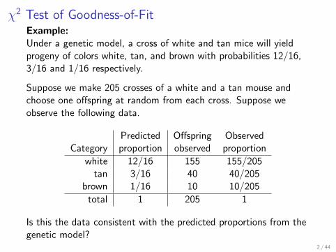
χ2 Test of Goodness-of-FitExample:Under a genetic model, a cross of white and tan mice will yieldprogeny of colors white, tan, and brown with probabilities 12/16,3/16 and 1/16 respectively.

Suppose we make 205 crosses of a white and a tan mouse andchoose one offspring at random from each cross. Suppose weobserve the following data.

Predicted Offspring ObservedCategory proportion observed proportion

white 12/16 155 155/205tan 3/16 40 40/205

brown 1/16 10 10/205

total 1 205 1

Is this the data consistent with the predicted proportions from thegenetic model?

2 / 44

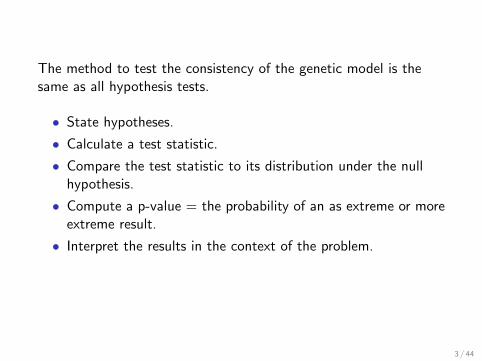
The method to test the consistency of the genetic model is thesame as all hypothesis tests.

• State hypotheses.

• Calculate a test statistic.

• Compare the test statistic to its distribution under the nullhypothesis.

• Compute a p-value = the probability of an as extreme or moreextreme result.

• Interpret the results in the context of the problem.

3 / 44

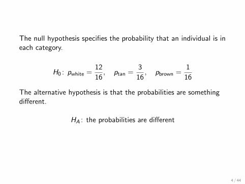
The null hypothesis specifies the probability that an individual is ineach category.

H0 : pwhite =12

16, ptan =

3

16, pbrown =

1

16

The alternative hypothesis is that the probabilities are somethingdifferent.

HA : the probabilities are different

4 / 44

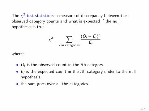
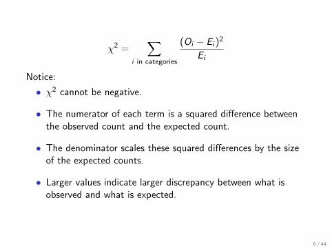
The χ2 test statistic is a measure of discrepancy between theobserved category counts and what is expected if the nullhypothesis is true.

χ2 =∑

i in categories

(Oi − Ei )2

Ei

where:

• Oi is the observed count in the ith category

• Ei is the expected count in the ith category under to the nullhypothesis.

• the sum goes over all the categories.

5 / 44

χ2 =∑

i in categories

(Oi − Ei )2

Ei

Notice:

• χ2 cannot be negative.

• The numerator of each term is a squared difference betweenthe observed count and the expected count.

• The denominator scales these squared differences by the sizeof the expected counts.

• Larger values indicate larger discrepancy between what isobserved and what is expected.

6 / 44

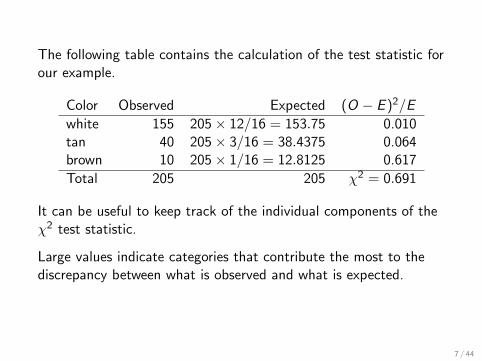
The following table contains the calculation of the test statistic forour example.

Color Observed Expected (O − E )2/E

white 155 205× 12/16 = 153.75 0.010tan 40 205× 3/16 = 38.4375 0.064brown 10 205× 1/16 = 12.8125 0.617

Total 205 205 χ2 = 0.691

It can be useful to keep track of the individual components of theχ2 test statistic.

Large values indicate categories that contribute the most to thediscrepancy between what is observed and what is expected.

7 / 44

Under the null hypothesis, the χ2 test statistic follows(approximately) a χ2 distribution with df degrees of freedom

where df = (number of categories)− 1.

• The distribution is not symmetric and only non-negativenumbers have positive probability.

• As df increases, the mean of the distribution increases, theskewness decreases, and the shape becomes more symmetricand normal.

8 / 44

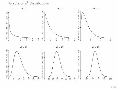
Graphs of χ2 Distributions

df = 1

0 1 2 3 4 5

0.0

0.5

1.0

1.5

2.0

2.5

df = 2

0 2 4 6 8 10

0.0

0.1

0.2

0.3

0.4

0.5

df = 3

0 5 10 150.00

0.05

0.10

0.15

0.20

0.25

df = 10

0 5 10 15 20 25 300.00

0.02

0.04

0.06

0.08

0.10

df = 30

0 10 20 30 40 50 60 700.00

0.01

0.02

0.03

0.04

0.05

df = 50

0 20 40 60 80 1000.00

0.01

0.02

0.03

0.04

9 / 44

• In the example, there are three categories and so our χ2

statistic has two degrees of freedom.

• The P-value is the probability of observing as extreme ormore extreme data.

Extreme data are far away from expected counts under thenull hypothesis.

Because the difference are squared more extreme means alarger χ2 value

10 / 44

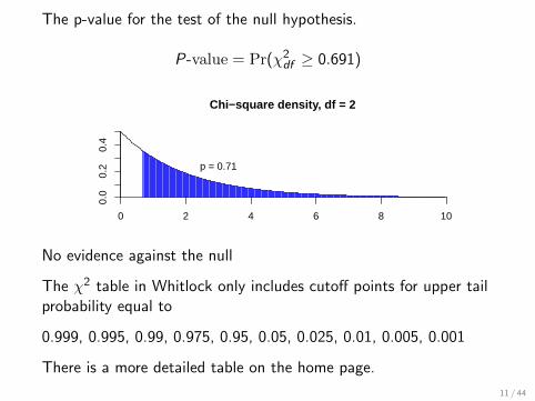
The p-value for the test of the null hypothesis.

P-value = Pr(χ2df ≥ 0.691)

Chi−square density, df = 2

0 2 4 6 8 10

0.0

0.2

0.4

p = 0.71

No evidence against the null

The χ2 table in Whitlock only includes cutoff points for upper tailprobability equal to

0.999, 0.995, 0.99, 0.975, 0.95, 0.05, 0.025, 0.01, 0.005, 0.001

There is a more detailed table on the home page.

11 / 44

The large p-value indicates that the data is consistent with the nullhypothesis. In the context of the problem,

There is no evidence against the null genetic model forthe color probabilities from the cross of white and tanmice. The observed data is consistent with the expected12:3:1 ratios. The difference between observed andexpected counts is easily explained by chance variation.

12 / 44

Assumptions

The chi-square statistic will follow the χ2 distribution with = n− 1degrees of freedom if:

• The data are a categorical variable measured on a simplerandom sample from a large population.

• The null hypothesis specifies the probabilities of each category.

• The expected counts are large enough:

- all categories have an expected count (Ei ) greater than 1- no more than 20% of the categories have Ei less than 5.

If these assumptions are met the p-value will be accurate.

13 / 44

Contingency tables

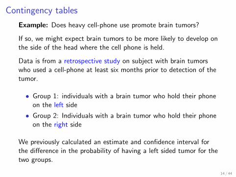
Example: Does heavy cell-phone use promote brain tumors?

If so, we might expect brain tumors to be more likely to develop onthe side of the head where the cell phone is held.

Data is from a retrospective study on subject with brain tumorswho used a cell-phone at least six months prior to detection of thetumor.

• Group 1: individuals with a brain tumor who hold their phoneon the left side

• Group 2: Individuals with a brain tumor who hold their phoneon the right side

We previously calculated an estimate and confidence interval forthe difference in the probability of having a left sided tumor for thetwo groups.

14 / 44

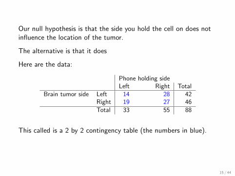
Our null hypothesis is that the side you hold the cell on does notinfluence the location of the tumor.

The alternative is that it does

Here are the data:

Phone holding sideLeft Right Total

Brain tumor side Left 14 28 42Right 19 27 46Total 33 55 88

This called is a 2 by 2 contingency table (the numbers in blue).

15 / 44

χ2 Test of independence

We have

• a simple random sample of brain tumor sufferers.

• a categorical variable with 4 possible outcomes measured oneach (the 4 possible cells in the table).

If we can calculate the expected number for each of the 4 cellsunder the null hypothesis the we can use a χ2 goodness of fit testto check that the data support the null hypothesis.

16 / 44

Under the null hypothesis the side you hold the cell on does notinfluence the location of the tumor.

This implies:

Pr(cell phone left AND tumor left|H0)

= Pr(cell phone left|H0)× Pr(tumor left|H0)

(Multiplication rule for independent events).

We can estimate

Pr(cell phone left|H0) and Pr(tumor left|H0)

using the table margins.

17 / 44

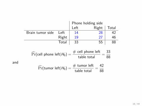
Phone holding sideLeft Right Total

Brain tumor side Left 14 28 42Right 19 27 46Total 33 55 88

P̂r(cell phone left|H0) =# cell phone left

table total=

33

88

and

P̂r(tumor left|H0) =# tumor left

table total=

42

88

18 / 44

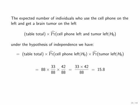
The expected number of individuals who use the cell phone on theleft and get a brain tumor on the left

(table total)× P̂r(cell phone left and tumor left|H0)

under the hypothesis of independence we have:

= (table total)× P̂r(cell phone left|H0)× P̂r(tumor left|H0)

= 88× 33

88× 42

88=

33× 42

88= 15.8

19 / 44

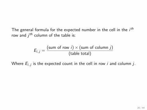
The general formula for the expected number in the cell in the i th

row and j th column of the table is:

Ei , j =(sum of row i)× (sum of column j)

(table total)

Where Ei , j is the expected count in the cell in row i and column j .

20 / 44

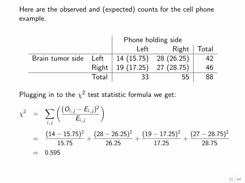
Here are the observed and (expected) counts for the cell phoneexample.

Phone holding sideLeft Right Total

Brain tumor side Left 14 (15.75) 28 (26.25) 42Right 19 (17.25) 27 (28.75) 46

Total 33 55 88

Plugging in to the χ2 test statistic formula we get:

χ2 =∑i, j

((Oi, j − Ei, j)

2

Ei, j

)

=(14− 15.75)2

15.75+

(28− 26.25)2

26.25+

(19− 17.25)2

17.25+

(27− 28.75)2

28.75

= 0.595

21 / 44

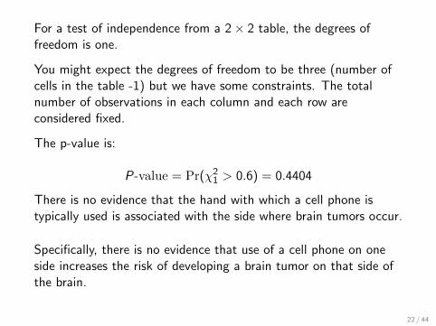
For a test of independence from a 2× 2 table, the degrees offreedom is one.

You might expect the degrees of freedom to be three (number ofcells in the table -1) but we have some constraints. The totalnumber of observations in each column and each row areconsidered fixed.

The p-value is:

P-value = Pr(χ21 > 0.6) = 0.4404

There is no evidence that the hand with which a cell phone istypically used is associated with the side where brain tumors occur.

Specifically, there is no evidence that use of a cell phone on oneside increases the risk of developing a brain tumor on that side ofthe brain.

22 / 44

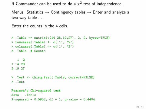
R Commander can be used to do a χ2 test of independence.

Menus: Statistics → Contingency tables → Enter and analyze atwo-way table ...

Enter the counts in the 4 cells.

> .Table <- matrix(c(14,28,19,27), 2, 2, byrow=TRUE)

> rownames(.Table) <- c(’1’, ’2’)

> colnames(.Table) <- c(’1’, ’2’)

> .Table # Counts

1 2

1 14 28

2 19 27

> .Test <- chisq.test(.Table, correct=FALSE)

> .Test

Pearson’s Chi-squared test

data: .Table

X-squared = 0.5952, df = 1, p-value = 0.4404

23 / 44

Hypothesis test for a difference in two proportions.

For the test of independence in a 2× 2 table the null hypothesis isthat the side you hold the cell on does not influence the location ofthe tumor.

An equivalent null hypothesis is that the proportion of tumors onthe left is the same for left and right cell phone holders

If

p1 = proportion of right cell phone holders with tumors on the left

and

p2 = proportion of left cell phone holders with tumors on the left

then the null hypothesis can be written H0 : p1 = p2

The hypothesis test for the difference in two proportions is exactlythe same as the χ2 test for independence in a 2x2 table.

24 / 44

Larger Tables

The χ2 test for independence extends easily to larger contingencytables.

ExampleA study examined the relative efficacy of penicillin andspectinomycin in treating gonorrhea.

Three treatments are considered:

• penicillin

• spectinomycin (low dose)

• spectinomycin (high dose)

Three possible responses are recorded:

• positive smear

• negative smear, positive culture

• negative smear, negative culture

25 / 44

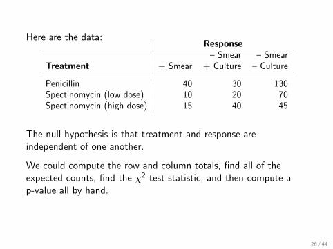
Here are the data:Response

– Smear – SmearTreatment + Smear + Culture – Culture

Penicillin 40 30 130Spectinomycin (low dose) 10 20 70Spectinomycin (high dose) 15 40 45

The null hypothesis is that treatment and response areindependent of one another.

We could compute the row and column totals, find all of theexpected counts, find the χ2 test statistic, and then compute ap-value all by hand.

26 / 44

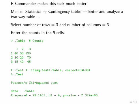
R Commander makes this task much easier.

Menus: Statistics → Contingency tables → Enter and analyze atwo-way table ...

Select number of rows = 3 and number of columns = 3

Enter the counts in the 9 cells.

> .Table # Counts

1 2 3

1 40 30 130

2 10 20 70

3 15 40 45

> .Test <- chisq.test(.Table, correct=FALSE)

> .Test

Pearson’s Chi-squared test

data: .Table

X-squared = 29.1401, df = 4, p-value = 7.322e-06

27 / 44

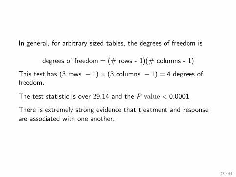
In general, for arbitrary sized tables, the degrees of freedom is

degrees of freedom = (# rows - 1)(# columns - 1)

This test has (3 rows − 1)× (3 columns − 1) = 4 degrees offreedom.

The test statistic is over 29.14 and the P-value < 0.0001

There is extremely strong evidence that treatment and responseare associated with one another.

28 / 44

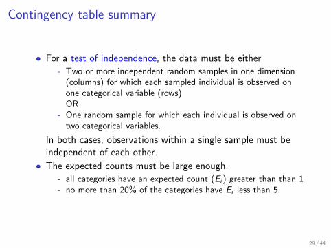
Contingency table summary

• For a test of independence, the data must be either

- Two or more independent random samples in one dimension(columns) for which each sampled individual is observed onone categorical variable (rows)OR

- One random sample for which each individual is observed ontwo categorical variables.

In both cases, observations within a single sample must beindependent of each other.

• The expected counts must be large enough.

- all categories have an expected count (Ei ) greater than than 1- no more than 20% of the categories have Ei less than 5.

29 / 44

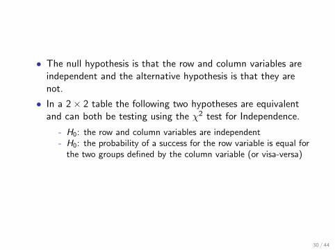
• The null hypothesis is that the row and column variables areindependent and the alternative hypothesis is that they arenot.

• In a 2× 2 table the following two hypotheses are equivalentand can both be testing using the χ2 test for Independence.

- H0: the row and column variables are independent- H0: the probability of a success for the row variable is equal for

the two groups defined by the column variable (or visa-versa)

30 / 44

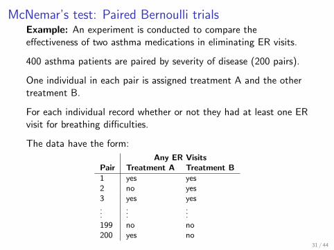
McNemar’s test: Paired Bernoulli trialsExample: An experiment is conducted to compare theeffectiveness of two asthma medications in eliminating ER visits.

400 asthma patients are paired by severity of disease (200 pairs).

One individual in each pair is assigned treatment A and the othertreatment B.

For each individual record whether or not they had at least one ERvisit for breathing difficulties.

The data have the form:

Any ER VisitsPair Treatment A Treatment B1 yes yes2 no yes3 yes yes...

......

199 no no200 yes no

31 / 44

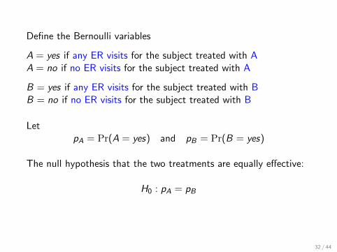
Define the Bernoulli variables

A = yes if any ER visits for the subject treated with AA = no if no ER visits for the subject treated with A

B = yes if any ER visits for the subject treated with BB = no if no ER visits for the subject treated with B

LetpA = Pr(A = yes) and pB = Pr(B = yes)

The null hypothesis that the two treatments are equally effective:

H0 : pA = pB

32 / 44

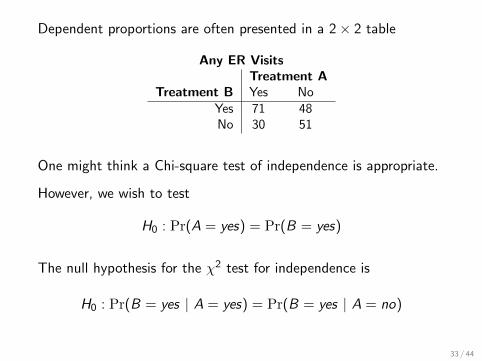
Dependent proportions are often presented in a 2× 2 table

Any ER VisitsTreatment A

Treatment B Yes NoYes 71 48No 30 51

One might think a Chi-square test of independence is appropriate.

However, we wish to test

H0 : Pr(A = yes) = Pr(B = yes)

The null hypothesis for the χ2 test for independence is

H0 : Pr(B = yes | A = yes) = Pr(B = yes | A = no)

33 / 44

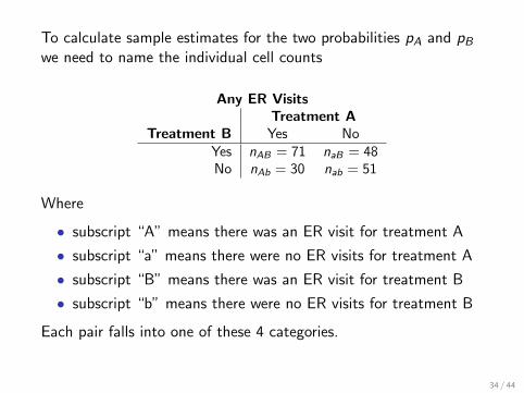
To calculate sample estimates for the two probabilities pA and pBwe need to name the individual cell counts

Any ER VisitsTreatment A

Treatment B Yes NoYes nAB = 71 naB = 48No nAb = 30 nab = 51

Where

• subscript “A” means there was an ER visit for treatment A

• subscript “a” means there were no ER visits for treatment A

• subscript “B” means there was an ER visit for treatment B

• subscript “b” means there were no ER visits for treatment B

Each pair falls into one of these 4 categories.

34 / 44

So, for example there are nAb = 30 pairs where:

The member of the pair receiving Treatment A had ER visits

and

The member of the pair receiving Treatment B had no ERvisits.

35 / 44

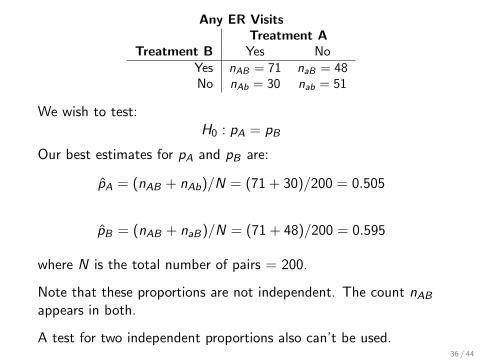
Any ER VisitsTreatment A

Treatment B Yes NoYes nAB = 71 naB = 48No nAb = 30 nab = 51

We wish to test:H0 : pA = pB

Our best estimates for pA and pB are:

p̂A = (nAB + nAb)/N = (71 + 30)/200 = 0.505

p̂B = (nAB + naB)/N = (71 + 48)/200 = 0.595

where N is the total number of pairs = 200.

Note that these proportions are not independent. The count nABappears in both.

A test for two independent proportions also can’t be used.36 / 44

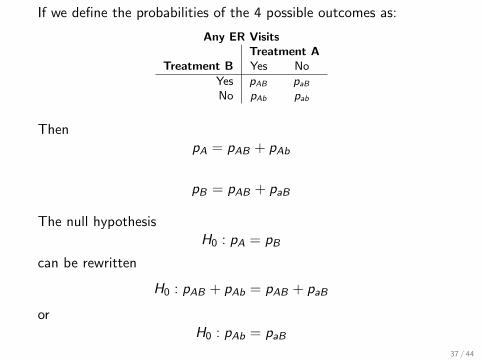
If we define the probabilities of the 4 possible outcomes as:

Any ER VisitsTreatment A

Treatment B Yes No

Yes pAB paBNo pAb pab

ThenpA = pAB + pAb

pB = pAB + paB

The null hypothesisH0 : pA = pB

can be rewritten

H0 : pAB + pAb = pAB + paB

orH0 : pAb = paB

37 / 44

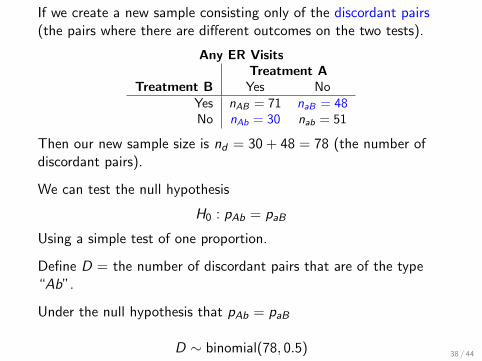
If we create a new sample consisting only of the discordant pairs(the pairs where there are different outcomes on the two tests).

Any ER VisitsTreatment A

Treatment B Yes NoYes nAB = 71 naB = 48No nAb = 30 nab = 51

Then our new sample size is nd = 30 + 48 = 78 (the number ofdiscordant pairs).

We can test the null hypothesis

H0 : pAb = paB

Using a simple test of one proportion.

Define D = the number of discordant pairs that are of the type“Ab”.

Under the null hypothesis that pAb = paB

D ∼ binomial(78, 0.5) 38 / 44

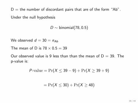
D = the number of discordant pairs that are of the form “Ab”.

Under the null hypothesis

D ∼ binomial(78, 0.5)

We observed d = 30 = nAb

The mean of D is 78× 0.5 = 39

Our observed value is 9 less than than the mean of D = 39. Thep-value is:

P-value = Pr(X ≤ 39− 9) + Pr(X ≥ 39 + 9)

= Pr(X ≤ 30) + Pr(X ≥ 48)

39 / 44

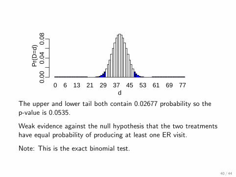
0 6 13 21 29 37 45 53 61 69 77d

Pr(

D=

d)0.

000.

040.

08

The upper and lower tail both contain 0.02677 probability so thep-value is 0.0535.

Weak evidence against the null hypothesis that the two treatmentshave equal probability of producing at least one ER visit.

Note: This is the exact binomial test.

40 / 44

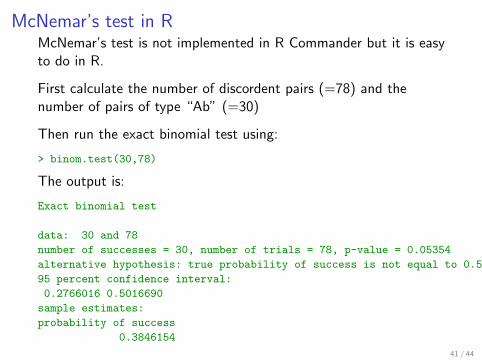
McNemar’s test in RMcNemar’s test is not implemented in R Commander but it is easyto do in R.

First calculate the number of discordent pairs (=78) and thenumber of pairs of type “Ab” (=30)

Then run the exact binomial test using:

> binom.test(30,78)

The output is:

Exact binomial test

data: 30 and 78

number of successes = 30, number of trials = 78, p-value = 0.05354

alternative hypothesis: true probability of success is not equal to 0.5

95 percent confidence interval:

0.2766016 0.5016690

sample estimates:

probability of success

0.3846154

41 / 44

Even easier is to use the calculator at

http://vassarstats.net/propcorr.html

Includes a description of McNemar’s test and a calculator (uses theexact binomial test).

Linked on the home page under reading for this lecture and under“Online Calculators”.

42 / 44

McNmear’s test vs. χ2 test of independence for 2× 2tables

McNemar’s test is used when we wish to compare the percentpositive for two variables measured on the same sampling units(paired Bernoulli trials).

Variable APositive Negative

Variable B = Positive nAB naBNegative nAb nab

Null hypothesis for McNemar’s test: H0 : pA = pB

pA is the probability that variable A is positivep̂A = (nAB + nAb)/N

pB is the probability that variable B is positivep̂B = (nAB + naB)/N

where N = (nAB + naB + nAb + nab)

43 / 44

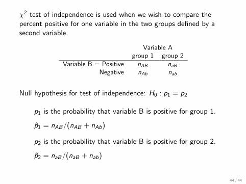
χ2 test of independence is used when we wish to compare thepercent positive for one variable in the two groups defined by asecond variable.

Variable Agroup 1 group 2

Variable B = Positive nAB naBNegative nAb nab

Null hypothesis for test of independence: H0 : p1 = p2

p1 is the probability that variable B is positive for group 1.

p̂1 = nAB/(nAB + nAb)

p2 is the probability that variable B is positive for group 2.

p̂2 = naB/(naB + nab)

44 / 44