Biological Image Analysis Primer - ImageScience.Org · 8 BIOLOGICAL IMAGE ANALYSIS PRIMER Figure...

Biological Image Analysis Primer

Erik Meijering∗ and Gert van Cappellen#

∗Biomedical Imaging Group#Applied Optical Imaging Center

Erasmus MC – University Medical CenterRotterdam, the Netherlands

Typeset by the authors using LATEX2ε.

Copyright c© 2006 by the authors. All rights reserved. No part of this bookletmay be reproduced or transmitted in any form or by any means, electronic ormechanical, including photocopy, recording, or any information storage andretrieval system, without permission in writing from the authors.

Preface

This booklet was written as a companion to the introductory lecture on digitalimage analysis for biological applications, given by the first author as part ofthe course In Vivo Imaging – From Molecule to Organism, which is organized an-nually by the second author and other members of the applied Optical Imag-ing Center (aOIC) under the auspices of the postgraduate school MolecularMedicine (MolMed) together with the Medical Genetics Center (MGC) of theErasmus MC in Rotterdam, the Netherlands. Avoiding technicalities as muchas possible, the text serves as a primer to introduce those active in biologicalinvestigation to common terms and principles related to image processing,image analysis, visualization, and software tools. Ample references to the rel-evant literature are provided for those interested in learning more.

Acknowledgments The authors are grateful to Adriaan Houtsmuller, NielsGaljart, Jeroen Essers, Carla da Silva Almeida, Remco van Horssen, and Timoten Hagen (Erasmus MC, Rotterdam, the Netherlands), Floyd Sarria and Har-ald Hirling (Swiss Federal Institute of Technology, Lausanne, Switzerland),Anne McKinney (McGill University, Montreal, Quebec, Canada), and Elisa-beth Rungger-Brandle (University Eye Clinic, Geneva, Switzerland) for pro-viding image data for illustrational purposes. The contribution of the first au-thor was financially supported by the Netherlands Organization for ScientificResearch (NWO), through VIDI-grant 639.022.401.

Contents

Preface 3

1 Introduction 51.1 Definition of Common Terms . . . . . . . . . . . . . . . . . . . . 51.2 Historical and Future Perspectives . . . . . . . . . . . . . . . . . 7

2 Image Processing 102.1 Intensity Transformation . . . . . . . . . . . . . . . . . . . . . . . 102.2 Local Image Filtering . . . . . . . . . . . . . . . . . . . . . . . . . 122.3 Geometrical Transformation . . . . . . . . . . . . . . . . . . . . . 152.4 Image Restoration . . . . . . . . . . . . . . . . . . . . . . . . . . . 15

3 Image Analysis 193.1 Colocalization Analysis . . . . . . . . . . . . . . . . . . . . . . . 193.2 Neuron Tracing and Quantification . . . . . . . . . . . . . . . . . 213.3 Particle Detection and Tracking . . . . . . . . . . . . . . . . . . . 233.4 Cell Segmentation and Tracking . . . . . . . . . . . . . . . . . . . 25

4 Visualization 264.1 Volume Rendering . . . . . . . . . . . . . . . . . . . . . . . . . . 264.2 Surface Rendering . . . . . . . . . . . . . . . . . . . . . . . . . . . 28

5 Software Tools 29

References 30

Index 35

1Introduction

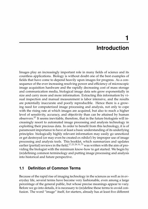
Images play an increasingly important role in many fields of science and itscountless applications. Biology is without doubt one of the best examples offields that have come to depend heavily upon images for progress. As a con-sequence of the ever increasing resolving power and efficiency of microscopicimage acquisition hardware and the rapidly decreasing cost of mass storageand communication media, biological image data sets grow exponentially insize and carry more and more information. Extracting this information by vi-sual inspection and manual measurement is labor intensive, and the resultsare potentially inaccurate and poorly reproducible. Hence there is a grow-ing need for computerized image processing and analysis, not only to copewith the rising rate at which images are acquired, but also to reach a higherlevel of sensitivity, accuracy, and objectivity than can be attained by humanobservers.57 It seems inevitable, therefore, that in the future biologists will in-creasingly resort to automated image processing and analysis technology inexploiting their precious data. In order to benefit from this technology, it is ofparamount importance to have at least a basic understanding of its underlyingprinciples: biologically highly relevant information may easily go unnoticedor get destroyed (or may even be created ex nihilo!) by improper use of imageprocessing and analysis tools. This booklet, which summarizes and updatesearlier (partial) reviews in the field,17, 23, 29, 31, 73 was written with the aim of pro-viding the biologist with the minimum know-how to get started. We begin by(re)defining common terminology and putting image processing and analysisinto historical and future perspective.

1.1 Definition of Common Terms

Because of the rapid rise of imaging technology in the sciences as well as in ev-eryday life, several terms have become very fashionable, even among a largepercentage of the general public, but whose precise meanings appear to vary.Before we go into details, it is necessary to (re)define these terms to avoid con-fusion. The word “image” itself, for starters, already has at least five different

6 BIOLOGICAL IMAGE ANALYSIS PRIMER

meanings. In the most general sense of the word, an image is a representationof something else. Depending on the type of representation, images can be di-vided into several classes.15 These include images perceivable by the humaneye, such as pictures (photographs, paintings, drawings) or those formed bylenses or holograms (optical images), as well as nonvisible images, such ascontinuous or discrete mathematical functions, or distributions of measurablephysical properties. In the remainder of this booklet, when we speak of animage, we mean a digital image, defined as a representation obtained by tak-ing finitely many samples, expressed as numbers that can take on only finitelymany values. In the present context of (in vivo) biological imaging, the objectswe make representations of are (living) cells and molecules, and the imagesare usually acquired by taking samples of (fluorescent or other) light at givenintervals in space and time and wavelength.

Mathematically speaking, images are matrices, or discrete functions, withthe number of dimensions typically ranging from one to five and where eachdimension corresponds to a parameter, a degree of freedom, or a coordinateneeded to uniquely locate a sample value (Figure 1.1). A description of how,exactly, these matrices are obtained and how they relate to the physical worldis outside the scope of this booklet but can be found elsewhere.61 Each sam-ple corresponds to what we call an image element. If the image is spatially2D, the elements are usually called pixels (short for “picture elements,” eventhough the image need not necessarily be a picture). In the case of spatially3D images, they are called voxels (“volume elements”). However, since datasets in optical microscopy usually consist of series of 2D images (time framesor optical sections) rather than truly volumetric images, we refer to an imageelement of any dimensionality as a “pixel” here.

Image processing is defined as the act of subjecting an image to a seriesof operations that alter its form or its value. The result of these operations isagain an image. This is distinct from image analysis, which is defined as theact of measuring (biologically) meaningful object features in an image. Mea-surement results can be either qualitative (categorical data) or quantitative(numerical data) and both types of results can be either subjective (depen-dent on the personal feelings and prejudices of the subject doing the measure-ments) or objective (solely dependent on the object itself and the measurementmethod). In many fields of research there is a tendency towards quantifica-tion and objectification, feeding the need for fully automated image analysismethods. Ultimately, image analysis results should lead to understanding thenature and interrelations of the objects being imaged. This requires not onlymeasurement data, but also reasoning about the data and making inferences,which involves some form of intelligence and cognitive processing. Comput-erizing these aspects of human vision is the long-term goal of computer vi-sion. Finally we mention computer graphics and visualization. These termsare strongly related,78 but strictly speaking the former refers to the process ofgenerating images for display of given data using a computer, while the latter

BIOLOGICAL IMAGE ANALYSIS PRIMER 7

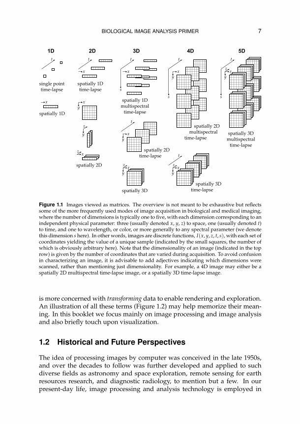
Figure 1.1 Images viewed as matrices. The overview is not meant to be exhaustive but reflectssome of the more frequently used modes of image acquisition in biological and medical imaging,where the number of dimensions is typically one to five, with each dimension corresponding to anindependent physical parameter: three (usually denoted x, y, z) to space, one (usually denoted t)to time, and one to wavelength, or color, or more generally to any spectral parameter (we denotethis dimension s here). In other words, images are discrete functions, I(x, y, z, t, s), with each set ofcoordinates yielding the value of a unique sample (indicated by the small squares, the number ofwhich is obviously arbitrary here). Note that the dimensionality of an image (indicated in the toprow) is given by the number of coordinates that are varied during acquisition. To avoid confusionin characterizing an image, it is advisable to add adjectives indicating which dimensions werescanned, rather than mentioning just dimensionality. For example, a 4D image may either be aspatially 2D multispectral time-lapse image, or a spatially 3D time-lapse image.

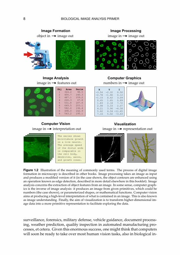
is more concerned with transforming data to enable rendering and exploration.An illustration of all these terms (Figure 1.2) may help memorize their mean-ing. In this booklet we focus mainly on image processing and image analysisand also briefly touch upon visualization.

1.2 Historical and Future Perspectives

The idea of processing images by computer was conceived in the late 1950s,and over the decades to follow was further developed and applied to suchdiverse fields as astronomy and space exploration, remote sensing for earthresources research, and diagnostic radiology, to mention but a few. In ourpresent-day life, image processing and analysis technology is employed in


Figure 1.2 Illustration of the meaning of commonly used terms. The process of digital imageformation in microscopy is described in other books. Image processing takes an image as inputand produces a modified version of it (in the case shown, the object contours are enhanced usingan operation known as edge detection, described in more detail elsewhere in this booklet). Imageanalysis concerns the extraction of object features from an image. In some sense, computer graph-ics is the inverse of image analysis: it produces an image from given primitives, which could benumbers (the case shown), or parameterized shapes, or mathematical functions. Computer visionaims at producing a high-level interpretation of what is contained in an image. This is also knownas image understanding. Finally, the aim of visualization is to transform higher-dimensional im-age data into a more primitive representation to facilitate exploring the data.

surveillance, forensics, military defense, vehicle guidance, document process-ing, weather prediction, quality inspection in automated manufacturing pro-cesses, et cetera. Given this enormous success, one might think that computerswill soon be ready to take over most human vision tasks, also in biological in-


vestigation. This is still far from becoming a reality, however. After 50 yearsof research, our knowledge of the human visual system and how to excel it isstill very fragmentary and mostly confined to the early stages, that is to imageprocessing and image analysis. It seems reasonable to predict that another 50years of multidisciplinary efforts involving vision research, psychology, math-ematics, physics, computer science, and artificial intelligence will be requiredbefore we can begin to build highly sophisticated computer vision systemsthat outperform human observers in all respects. In the meantime, however,currently available methods may already be of great help in reducing manuallabor and increasing accuracy, objectivity, and reproducibility.

2Image Processing

Several fundamental image processing operations have been developed overthe past decades that appear time and again as part of more involved imageprocessing and analysis procedures. Here we discuss four classes of opera-tions that are most commonly used: intensity transformation, linear and non-linear image filtering, geometrical transformation, and image restoration. Forease of illustration, examples are given for spatially 2D images, but they eas-ily extend to higher-dimensional images. Also, the examples are confined tointensity (gray-scale) images. In the case of multispectral images, some oper-ations may need to be applied separately to each channel, possibly with dif-ferent parameter settings. A more elaborate treatment of the mentioned (andother) basic image processing operations can be found in the cited works andin a variety of textbooks.7, 15, 33, 38, 39, 72, 81

2.1 Intensity Transformation

Among the simplest image processing operations are those that pass alongeach image pixel and produce an output value that depends only on the cor-responding input value and some mapping function. These are also calledpoint operations. If the mapping function is the same for each pixel, we speakof a global intensity transformation. An infinity of mapping functions can bedevised, but most often a (piecewise) linear function is used, which allowseasy (interactive) adjustment of image brightness and contrast. Two extremesof this operation are intensity inversion and intensity thresholding. The lat-ter is one of the easiest (and most error-prone!) approaches to divide an imageinto meaningful objects and background, a task referred to as image segmenta-tion. Logarithmic mapping functions are also sometimes used to better matchthe light sensitivity of the human eye when displaying images. Another typeof intensity transformation is pseudo-coloring. Since the human eye is moresensitive to changes in color than to changes in intensity, more detail may beperceived when mapping intensities to colors.


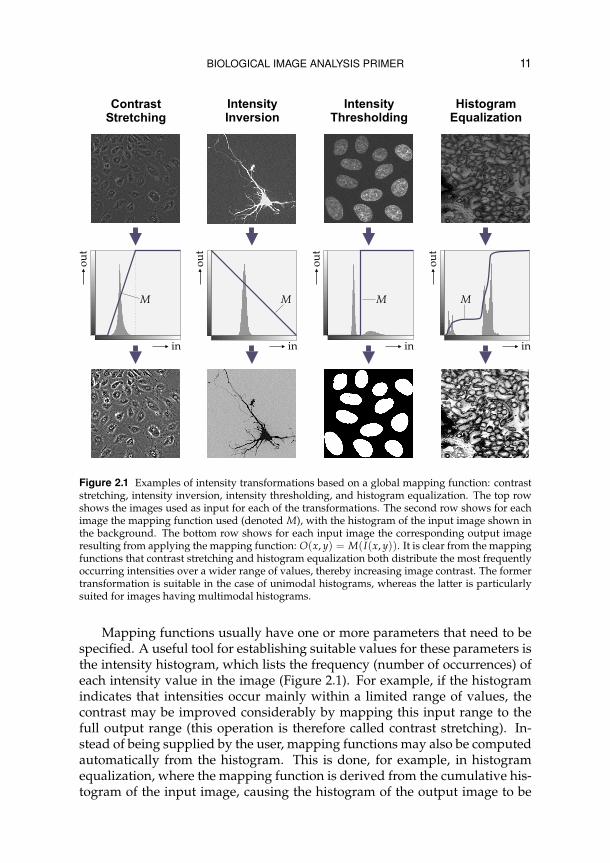
Figure 2.1 Examples of intensity transformations based on a global mapping function: contraststretching, intensity inversion, intensity thresholding, and histogram equalization. The top rowshows the images used as input for each of the transformations. The second row shows for eachimage the mapping function used (denoted M), with the histogram of the input image shown inthe background. The bottom row shows for each input image the corresponding output imageresulting from applying the mapping function: O(x, y) = M(I(x, y)). It is clear from the mappingfunctions that contrast stretching and histogram equalization both distribute the most frequentlyoccurring intensities over a wider range of values, thereby increasing image contrast. The formertransformation is suitable in the case of unimodal histograms, whereas the latter is particularlysuited for images having multimodal histograms.

Mapping functions usually have one or more parameters that need to bespecified. A useful tool for establishing suitable values for these parameters isthe intensity histogram, which lists the frequency (number of occurrences) ofeach intensity value in the image (Figure 2.1). For example, if the histogramindicates that intensities occur mainly within a limited range of values, thecontrast may be improved considerably by mapping this input range to thefull output range (this operation is therefore called contrast stretching). In-stead of being supplied by the user, mapping functions may also be computedautomatically from the histogram. This is done, for example, in histogramequalization, where the mapping function is derived from the cumulative his-togram of the input image, causing the histogram of the output image to be


more uniformly distributed. In cases where the intensity histogram is multi-modal, this operation may be more effective in improving image contrast be-tween different types of adjacent tissues than simple contrast stretching. Thehistogram may also be used to determine a global threshold value,30 for exam-ple the value corresponding to the minimum between the two major modesof the (smoothed) histogram, or the value that maximizes the interclass vari-ance (or, equivalently, minimizes the intraclass variance) of object (above thethreshold) and background (below the threshold) values.60

2.2 Local Image Filtering

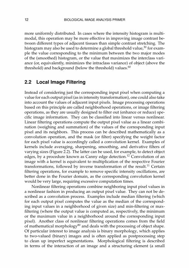
Instead of considering just the corresponding input pixel when computing avalue for each output pixel (as in intensity transformation), one could also takeinto account the values of adjacent input pixels. Image processing operationsbased on this principle are called neighborhood operations, or image filteringoperations, as they are usually designed to filter out (enhance or reduce) spe-cific image information. They can be classified into linear versus nonlinear.Linear filtering operations compute the output pixel value as a linear combi-nation (weighing and summation) of the values of the corresponding inputpixel and its neighbors. This process can be described mathematically as aconvolution operation, and the mask (or filter) specifying the weight factorfor each pixel value is accordingly called a convolution kernel. Examples ofkernels include averaging, sharpening, smoothing, and derivative filters ofvarying sizes (Figure 2.2). The latter can be used, for example, to detect objectedges, by a procedure known as Canny edge detection.12 Convolution of animage with a kernel is equivalent to multiplication of the respective Fouriertransformations, followed by inverse transformation of the result.11 Certainfiltering operations, for example to remove specific intensity oscillations, arebetter done in the Fourier domain, as the corresponding convolution kernelwould be very large, requiring excessive computation times.

Nonlinear filtering operations combine neighboring input pixel values ina nonlinear fashion in producing an output pixel value. They can not be de-scribed as a convolution process. Examples include median filtering (whichfor each output pixel computes the value as the median of the correspond-ing input values in a neighborhood of given size) and min-filtering or max-filtering (where the output value is computed as, respectively, the minimumor the maximum value in a neighborhood around the corresponding inputpixel). Another class of nonlinear filtering operations comes from the fieldof mathematical morphology80 and deals with the processing of object shape.Of particular interest to image analysis is binary morphology, which appliesto two-valued (binary) images and is often applied as postprocessing stepto clean up imperfect segmentations. Morphological filtering is describedin terms of the interaction of an image and a structuring element (a small


Figure 2.2 Principles and examples of convolution filtering. The value of an output pixel is com-puted as a linear combination (weighing and summation) of the value of the corresponding inputpixel and of its neighbors. The weight factor assigned to each input pixel is given by the convo-lution kernel (denoted K). In principle, kernels can be of any size. Examples of commonly usedkernels of size 3× 3 pixels include the averaging filter, the sharpening filter, and the Sobel x- ory-derivative filters. The Gaussian filter is often used as a smoothing filter. It has a free parameter(standard deviation σ) which determines the size of the kernel (usually cut off at m = 3σ) andtherefore the degree of smoothing. The derivatives of this kernel are often used to compute imagederivatives at different scales, as for example in Canny edge detection. The scale parameter, σ,should be chosen such that the resulting kernel matches the structures to be filtered.


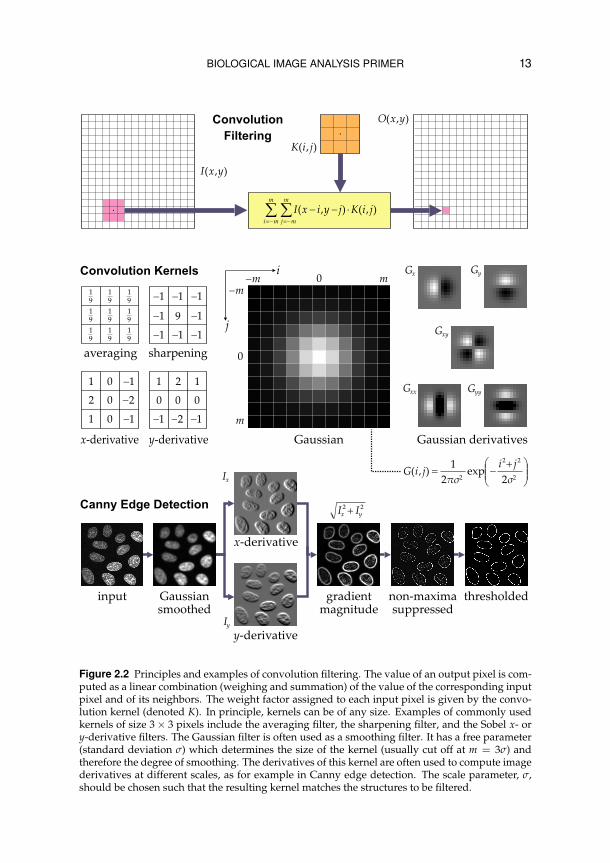
Figure 2.3 Principles and examples of binary morphological filtering. An object in the image isdescribed as the set (denoted X) of all coordinates of pixels belonging to that object. Morphologi-cal filters process this set using a second set, known as the structuring element (denoted S). Herethe discussion is limited to structuring elements that are symmetrical with respect to their centerelement, s = (0, 0), indicated by the dot. In that case, the dilation of X is defined as the set of allcoordinates x for which the cross section of S placed at x (denoted Sx) with X is not empty, and theerosion of X as the set of all x for which Sx is a subset of X. A dilation followed by an erosion (orvice versa) is called a closing (versus opening). These operations are named after the effects theyproduce, as illustrated. Many interesting morphological filters can be constructed by taking dif-ferences of two or more operations, such as in morphological edge detection. Other applicationsinclude skeletonization, which consists in a sequence of thinning operations producing the basicshape of objects, and granulometry, which uses a family of opening operations with increasinglylarger structuring elements to compute the size distribution of objects in an image.


mask reminiscent of a convolution kernel in the case of linear filtering). Ba-sic morphological operations include erosion, dilation, opening, and closing(Figure 2.3). By combining these we can design many interesting filters toprepare for (or even perform) image analysis. For example, subtracting the re-sults of dilation and erosion yields object edges. Or by analyzing the results ofa family of openings, using increasingly larger structuring elements, we mayperform size distribution analysis or granulometry of image structures. An-other operation that is frequently used in biological shape analysis24, 35, 36, 91 isskeletonization, which yields the basic shape of segmented objects.

2.3 Geometrical Transformation

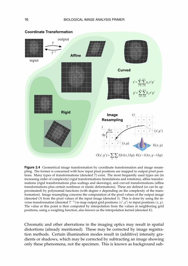
In many situations it may occur that the images acquired by the microscopeare spatially distorted or lack spatial correspondence. In colocalization exper-iments, for example, images of the same specimen imaged at different wave-lengths may show mismatches due to chromatic aberration. Nonlinear magni-fication from the center to the edge of the field of view may result in deforma-tions known as barrel distortion or pincushion distortion. In live cell exper-iments, one may be interested in studying specific intracellular componentsover time, which appear in different places in each image due to the motionof the cell itself. Such studies require image alignment, also referred to as im-age registration in the literature.45, 64, 82 Other studies, for example karyotypeanalyses, require the contents of images to be reformatted to some predefinedconfiguration. This is also known as image reformatting.

In all such cases, the images (or parts thereof) need to undergo spatial (orgeometrical) transformation prior to further processing or analysis. There aretwo aspects to this type of operation: coordinate transformation and imageresampling. The former concerns the mapping of input pixel positions to out-put pixel positions (and vice versa). Depending on the complexity of the prob-lem, one commonly uses a rigid, or an affine, or a curved transformation (Fig-ure 2.4). Image resampling concerns the issue of computing output pixel val-ues based on the input pixel values and the coordinate transformation. This isalso known as image interpolation, for which many methods exist. It is impor-tant to realize that every time an image is resampled, some information is lost.Studies in the field of medical imaging52, 85 have indicated that higher-orderspline interpolation methods (for example cubic splines) are much less harm-ful in this regard than some standard approaches, such as nearest-neighborinterpolation and linear interpolation, although the increased computationalload may be prohibitive in some applications.

2.4 Image Restoration

There are many factors in the acquisition process that cause a degradation ofimage quality in one way or another, resulting in a corrupted view of reality.


Figure 2.4 Geometrical image transformation by coordinate transformation and image resam-pling. The former is concerned with how input pixel positions are mapped to output pixel posi-tions. Many types of transformations (denoted T) exist. The most frequently used types are (inincreasing order of complexity) rigid transformations (translations and rotations), affine transfor-mations (rigid transformations plus scalings and skewings), and curved transformations (affinetransformations plus certain nonlinear or elastic deformations). These are defined (or can be ap-proximated) by polynomial functions (with degree n depending on the complexity of the trans-formation). Image resampling concerns the computation of the pixel values of the output image(denoted O) from the pixel values of the input image (denoted I). This is done by using the in-verse transformation (denoted T−1) to map output grid positions (x′, y′) to input positions (x, y).The value at this point is then computed by interpolation from the values at neighboring gridpositions, using a weighing function, also known as the interpolation kernel (denoted K).

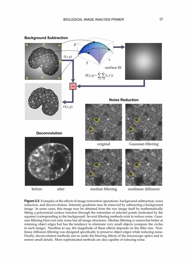
Chromatic and other aberrations in the imaging optics may result in spatialdistortions (already mentioned). These may be corrected by image registra-tion methods. Certain illumination modes result in (additive) intensity gra-dients or shadows, which may be corrected by subtracting an image showingonly these phenomena, not the specimen. This is known as background sub-


Figure 2.5 Examples of the effects of image restoration operations: background subtraction, noisereduction, and deconvolution. Intensity gradients may be removed by subtracting a backgroundimage. In some cases, this image may be obtained from the raw image itself by mathematicallyfitting a polynomial surface function through the intensities at selected points (indicated by thesquares) corresponding to the background. Several filtering methods exist to reduce noise. Gaus-sian filtering blurs not only noise but all image structures. Median filtering is somewhat better atretaining object edges but has the tendency to eliminate very small objects (compare the circlesin each image). Needless to say, the magnitude of these effects depends on the filter size. Non-linear diffusion filtering was designed specifically to preserve object edges while reducing noise.Finally, deconvolution methods aim to undo the blurring effects of the microscope optics and torestore small details. More sophisticated methods are also capable of reducing noise.


traction. If it is not possible to capture a background image, it may in somecases be obtained from the image to be corrected (Figure 2.5). Another ma-jor source of intensity corruption is noise, due to the quantum nature of light(signal-dependent noise, following Poisson statistics) and imperfect electron-ics (mostly signal-independent, Gaussian noise). One way to reduce noise islocal averaging of pixel intensities using a uniform or Gaussian convolutionfilter. However, while improving the overall signal-to-noise ratio (SNR), thisoperation also blurs other image structures. Median filtering is an effectiveway to remove shot noise (as caused, for example, by bright or dark pixels). Itshould be used with great care, however, when small objects are studied (suchas in particle tracking), as these may also be (partially) filtered out. A more so-phisticated technique is nonlinear diffusion filtering,63 which smoothes noisewhile preserving sharpness at object edges, by taking into account local imageproperties (notably the gradient magnitude).

Especially widefield microscopy images may suffer from excessive blur-ring due to out-of-focus light. But even in confocal microscopy, where mostof these effects are suppressed, images are blurred due to optical diffractioneffects.10, 34 To good accuracy, these effects may be modeled mathematicallyas a convolution of the true optical image with the 3D point-spread function(PSF) of the microscope optics. Methods that try to undo this operation, inother words that try in every point in the image to reassign light to the properin-focus location, are therefore called deconvolution methods.40, 61, 90 Simpleexamples include nearest-neighbor or multi-neighbor deblurring and Fourier-based inverse filtering methods. These are computationally fast but have thetendency to amplify noise. More sophisticated methods, which also reducenoise, are based on iterative regularization and other (constrained or statis-tical) iterative algorithms. In principle, deconvolution preserves total signalintensity while improving contrast by restoring signal position. Therefore it isoften desirable prior to quantitative image analysis.

3Image Analysis

The image processing operations described in the previous chapter are impor-tant in enhancing or correcting image data, but by themselves do not answerany specific biological questions. Addressing such questions requires muchmore involved image processing and analysis algorithms, consisting of se-ries of operations working closely together in “interrogating” the data andextracting biologically meaningful information. Because of the complexity ofbiological phenomena and the variability (or even ambiguity) of biologicalimage data, many analysis tasks are difficult to automate fully and requireexpert user input or interaction. In contrast with most image processing op-erations, image analysis methods are therefore often semi-automatic. Herewe briefly describe state-of-the-art methods for some of the most relevant andpressing image analysis problems in biology today: colocalization analysis,neuron tracing and quantification, and the detection or segmentation, track-ing and motion analysis of particles and cells. Several technical challenges inthese areas are still vigorously researched.

3.1 Colocalization Analysis

An interesting question in many biological studies is to what degree two ormore molecular species (typically proteins) are active in the same specimen.This co-occurrence phenomenon can be imaged by using a different fluores-cent label for each species, combined with multicolor optical microscopy imag-ing. A more specific question is whether or not proteins reside in the same(or proximate) physical locations in the specimen. This is the problem ofcolocalization. For such experiments it is of paramount importance that theemission spectra (rather than just the peak wavelengths) of the fluorophoresare sufficiently well separated and that the correct filter sets are used duringacquisition to reduce artifacts due to spectral bleed-through or fluorescenceresonance energy transfer (FRET) as much as possible. Quantitative colocal-ization is perhaps the most extreme example of image analysis: it takes twoimages (typically containing millions of pixels) and produces only a few num-


Figure 3.1 See description on page 21.

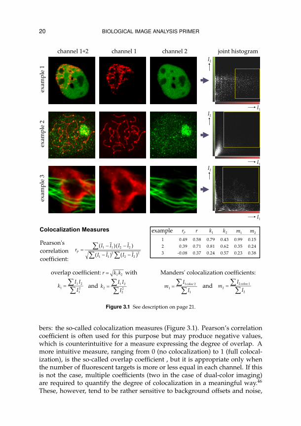
bers: the so-called colocalization measures (Figure 3.1). Pearson’s correlationcoefficient is often used for this purpose but may produce negative values,which is counterintuitive for a measure expressing the degree of overlap. Amore intuitive measure, ranging from 0 (no colocalization) to 1 (full colocal-ization), is the so-called overlap coefficient , but it is appropriate only whenthe number of fluorescent targets is more or less equal in each channel. If thisis not the case, multiple coefficients (two in the case of dual-color imaging)are required to quantify the degree of colocalization in a meaningful way.46

These, however, tend to be rather sensitive to background offsets and noise,


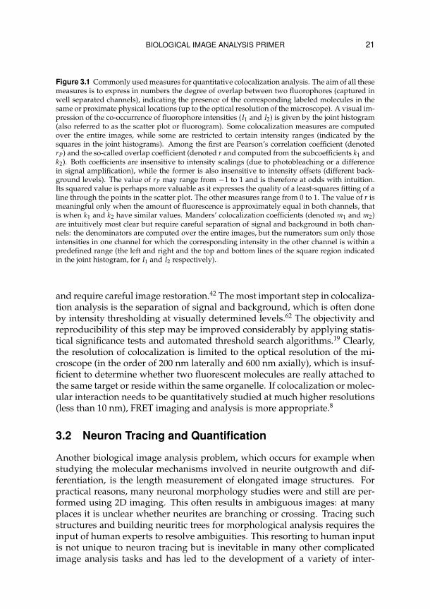
Figure 3.1 Commonly used measures for quantitative colocalization analysis. The aim of all thesemeasures is to express in numbers the degree of overlap between two fluorophores (captured inwell separated channels), indicating the presence of the corresponding labeled molecules in thesame or proximate physical locations (up to the optical resolution of the microscope). A visual im-pression of the co-occurrence of fluorophore intensities (I1 and I2) is given by the joint histogram(also referred to as the scatter plot or fluorogram). Some colocalization measures are computedover the entire images, while some are restricted to certain intensity ranges (indicated by thesquares in the joint histograms). Among the first are Pearson’s correlation coefficient (denotedrP) and the so-called overlap coefficient (denoted r and computed from the subcoefficients k1 andk2). Both coefficients are insensitive to intensity scalings (due to photobleaching or a differencein signal amplification), while the former is also insensitive to intensity offsets (different back-ground levels). The value of rP may range from −1 to 1 and is therefore at odds with intuition.Its squared value is perhaps more valuable as it expresses the quality of a least-squares fitting of aline through the points in the scatter plot. The other measures range from 0 to 1. The value of r ismeaningful only when the amount of fluorescence is approximately equal in both channels, thatis when k1 and k2 have similar values. Manders’ colocalization coefficients (denoted m1 and m2)are intuitively most clear but require careful separation of signal and background in both chan-nels: the denominators are computed over the entire images, but the numerators sum only thoseintensities in one channel for which the corresponding intensity in the other channel is within apredefined range (the left and right and the top and bottom lines of the square region indicatedin the joint histogram, for I1 and I2 respectively).

and require careful image restoration.42 The most important step in colocaliza-tion analysis is the separation of signal and background, which is often doneby intensity thresholding at visually determined levels.62 The objectivity andreproducibility of this step may be improved considerably by applying statis-tical significance tests and automated threshold search algorithms.19 Clearly,the resolution of colocalization is limited to the optical resolution of the mi-croscope (in the order of 200 nm laterally and 600 nm axially), which is insuf-ficient to determine whether two fluorescent molecules are really attached tothe same target or reside within the same organelle. If colocalization or molec-ular interaction needs to be quantitatively studied at much higher resolutions(less than 10 nm), FRET imaging and analysis is more appropriate.8

3.2 Neuron Tracing and Quantification

Another biological image analysis problem, which occurs for example whenstudying the molecular mechanisms involved in neurite outgrowth and dif-ferentiation, is the length measurement of elongated image structures. Forpractical reasons, many neuronal morphology studies were and still are per-formed using 2D imaging. This often results in ambiguous images: at manyplaces it is unclear whether neurites are branching or crossing. Tracing suchstructures and building neuritic trees for morphological analysis requires theinput of human experts to resolve ambiguities. This resorting to human inputis not unique to neuron tracing but is inevitable in many other complicatedimage analysis tasks and has led to the development of a variety of inter-


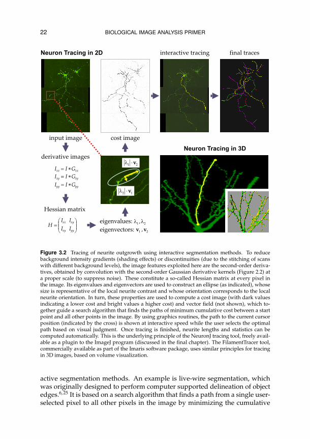
Figure 3.2 Tracing of neurite outgrowth using interactive segmentation methods. To reducebackground intensity gradients (shading effects) or discontinuities (due to the stitching of scanswith different background levels), the image features exploited here are the second-order deriva-tives, obtained by convolution with the second-order Gaussian derivative kernels (Figure 2.2) ata proper scale (to suppress noise). These constitute a so-called Hessian matrix at every pixel inthe image. Its eigenvalues and eigenvectors are used to construct an ellipse (as indicated), whosesize is representative of the local neurite contrast and whose orientation corresponds to the localneurite orientation. In turn, these properties are used to compute a cost image (with dark valuesindicating a lower cost and bright values a higher cost) and vector field (not shown), which to-gether guide a search algorithm that finds the paths of minimum cumulative cost between a startpoint and all other points in the image. By using graphics routines, the path to the current cursorposition (indicated by the cross) is shown at interactive speed while the user selects the optimalpath based on visual judgment. Once tracing is finished, neurite lengths and statistics can becomputed automatically. This is the underlying principle of the NeuronJ tracing tool, freely avail-able as a plugin to the ImageJ program (discussed in the final chapter). The FilamentTracer tool,commercially available as part of the Imaris software package, uses similar principles for tracingin 3D images, based on volume visualization.

active segmentation methods. An example is live-wire segmentation, whichwas originally designed to perform computer supported delineation of objectedges.6, 25 It is based on a search algorithm that finds a path from a single user-selected pixel to all other pixels in the image by minimizing the cumulative


value of a predefined cost function, computed from local image features (suchas gradient magnitude) along the path. The user can then interactively selectthe path that according to his own judgment best follows the structure of in-terest and fix the tracing up to some point, from where the process is iterateduntil the entire structure is traced. This technique has been adapted to enabletracing of neurite-like image structures in 2D and similar methods have beenapplied to neuron tracing in 3D (Figure 3.2).50 More automated methods for3D neuron tracing have also been published.24, 35, 77 In the case of poor imagequality, however, these may require manual postprocessing.

3.3 Particle Detection and Tracking

One of the major challenges of biomedical research in the postgenomic erais the unraveling of not just the spatial, but the spatiotemporal relationshipsof complex biomolecular systems.89 Naturally this involves the acquisition oftime-lapse image series and the tracking of objects over time. From an imageanalysis point of view, a distinction can be made between tracking of singlemolecules (or complexes) and tracking of entire cells (see next section). Anumber of tools are available for studying the dynamics of proteins based onfluorescent labeling and time-lapse imaging, such as fluorescence recovery af-ter (and loss in) photobleaching (FRAP and FLIP respectively), but these yieldonly ensemble average measurements of properties. More detailed studiesinto the different modes of motion of subpopulations require single particletracking,65, 75 which aims at motion analysis of individual proteins or micro-spheres. Computerized image analysis methods for this purpose have beendeveloped since the early 1990s and are constantly being improved5, 21 to dealwith increasingly sophisticated biological experimentation.

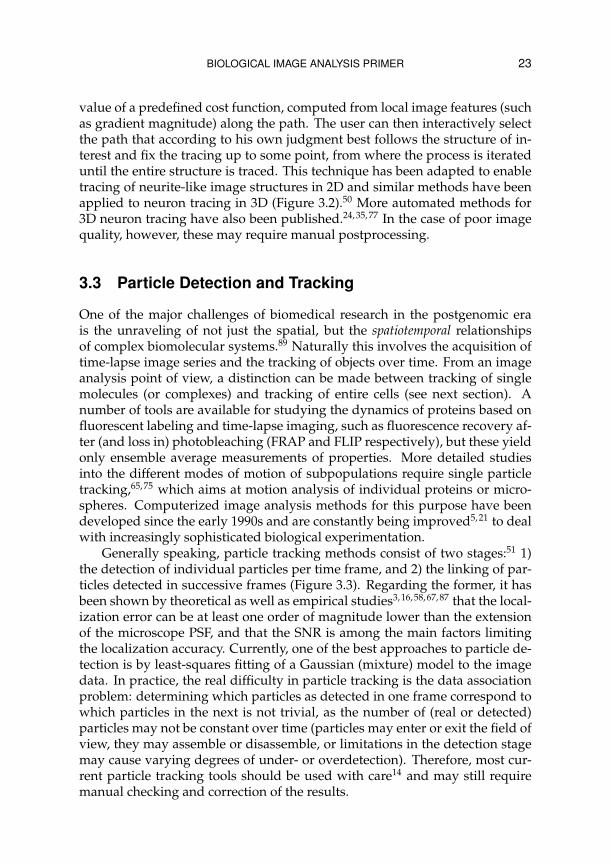
Generally speaking, particle tracking methods consist of two stages:51 1)the detection of individual particles per time frame, and 2) the linking of par-ticles detected in successive frames (Figure 3.3). Regarding the former, it hasbeen shown by theoretical as well as empirical studies3, 16, 58, 67, 87 that the local-ization error can be at least one order of magnitude lower than the extensionof the microscope PSF, and that the SNR is among the main factors limitingthe localization accuracy. Currently, one of the best approaches to particle de-tection is by least-squares fitting of a Gaussian (mixture) model to the imagedata. In practice, the real difficulty in particle tracking is the data associationproblem: determining which particles as detected in one frame correspond towhich particles in the next is not trivial, as the number of (real or detected)particles may not be constant over time (particles may enter or exit the field ofview, they may assemble or disassemble, or limitations in the detection stagemay cause varying degrees of under- or overdetection). Therefore, most cur-rent particle tracking tools should be used with care14 and may still requiremanual checking and correction of the results.


Figure 3.3 Challenges in particle and cell tracking. Regarding particle tracking, currently oneof the best approaches to detection of fluorescent tags is by least-squares fitting of a model ofthe intensity distribution to the image data. Because the tags are subresolution particles, theyappear as diffraction-limited spots in the images and therefore can be modeled well by a mixtureof Gaussian functions, each with its own amplitude scaling factor, standard deviation, and centerposition. Usually the detection is done separately for each time step, resulting in a list of potentialparticle positions and corresponding features, to be linked between time steps. The linking ishampered by the fact that the number of detected particles may be different for each time step. Incell tracking, a contour model (surface model in the case of 3D time-lapse experiments) is oftenused for segmentation. Commonly used models consist of control points, which are interpolatedusing smooth basis functions (typically B-splines) to form continuous, closed curves. The modelmust be flexible enough to handle geometrical as well as topological shape changes (cell division).The fitting is done by (constrained) movement of the control points to minimize some predefinedenergy functional computed from image-dependent information (intensity distributions insideand outside the curve) as well as image-independent information (a priori knowledge about cellshape and dynamics). Finally, trajectories can be visualized by representing them as tubes (seg-ments) and spheres (time points) and using surface rendering.


3.4 Cell Segmentation and Tracking

Motion estimation of cells is another frequently occurring problem in biolog-ical research. In particle tracking studies, for example, cell movement maymuddle the motion analysis of intracellular components and needs to be cor-rected for. In some cases, this may be accomplished by applying (nonrigid) im-age registration methods.23, 29, 70, 82 Cell migrations and deformations are alsointeresting in their own right, however, because of their role in a number ofbiological processes, including immune response, wound healing, embryonicdevelopment, and cancer metastasis.18 Understanding these processes is ofmajor importance in developing drugs or therapies to combat various typesof human disease. Typical 3D time-lapse data sets acquired for studies in thisarea consist of thousands of images and are almost impossible to analyze man-ually, both from a cost-efficiency perspective and because visual inspectionlacks the sensitivity, accuracy, and reproducibility needed to detect subtle butpotentially important phenomena. Therefore, computerized, quantitative celltracking and motion analysis is a requisite.22, 92

Contrary to single molecules or molecular complexes, which are subreso-lution objects appearing as PSF-shaped spots in the images, cells are relatively(with respect to pixel size) large objects, having a distinct shape. Detecting(or segmenting) entire cells and tracking position and shape changes requiresquite different image processing methods. Due to noise and photobleachingeffects, simple methods based on intensity thresholding are generally inade-quate. To deal with these artifacts and with obscure boundaries in the caseof touching cells, recent research has focused on the use of model-based seg-mentation methods,41, 48 which allow the incorporation of prior knowledgeabout object shape. Examples of such methods are active contours (also calledsnakes) and surfaces, which have been applied to a number of cell track-ing problems.20, 22, 69 They involve mathematical, prototypical shape descrip-tions having a limited number of degrees of freedom, which enable shape-constrained fitting to the image data based on data-dependent information(image properties, in particular intensity gradient information) and data-inde-pendent information (prior knowledge about the shape). Tracking is achievedby using the contour or surface obtained for one image as initialization for thenext, and repeating the fitting procedure (Figure 3.3).

4Visualization

Advances in imaging technology are rapidly turning higher-dimensional im-age data acquisition into the rule rather than the exception. Consequently,there is an increasing need for sophisticated visualization technology to en-able efficient presentation and exploration of this data and associated imageanalysis results. Early systems supported browsing the data in a frame-by-frame fashion,88 which provided only limited insight into the interrelations ofobjects in the images. Since visualization means generating representationsof higher-dimensional data, this necessarily implies reducing dimensionalityand possibly even reducing information in some sensible way. Exactly how todo this optimally depends on the application, the dimensionality of the data,and the physical nature of its respective dimensions (Figure 1.1). In any case,visualization methods usually consist of highly sophisticated information pro-cessing steps that may have a strong influence on the final result, making themvery susceptible to misuse. Here we briefly explain the two main modes of vi-sualization and point at critical steps in the process. More information can befound in textbooks on visualization and computer graphics.27, 78

4.1 Volume Rendering

Visualization methods that produce a viewable image of higher-dimensionalimage data without requiring an explicit geometrical representation of thatdata are called volume rendering methods. A commonly used, flexible andeasy to understand volume rendering method is ray casting, or ray tracing.With this method, the value of each pixel in the view image is determined by“casting a ray” into the image data and evaluating the data encountered alongthat ray using a predefined ray function (Figure 4.1). The direction of the raysis determined by the viewing angles and the mode of projection, which canbe orthographic (the rays run parallel to each other) or perspective (the rayshave a common focal point). Analogous to the real-world situation, these arecalled camera properties. The rays pass through the data with a certain stepsize, which should be smaller than the pixel size to avoid skipping impor-


Figure 4.1 Visualization of volumetric image data using volume rendering and surface renderingmethods. Volume rendering methods do not require an explicit geometrical representation ofthe objects of interest present in the data. A commonly used volume rendering method is raycasting: for each pixel in the view image, a ray is cast into the data, and the intensity profilealong the ray is fed to a ray function, which determines the output value, such as the maximum,average, or minimum intensity, or accumulated “opacity” (derived from intensity or gradientmagnitude information). By contrast, surface rendering methods require a segmentation of theobjects (usually obtained by thresholding), from which a surface representation (triangulation)is derived, allowing very fast rendering by graphics hardware. To reduce the effects of noise,Gaussian smoothing is often applied as a preprocessing step prior to segmentation. As shown,both operations have a substantial influence on the final result: by slightly changing the degreeof smoothing or the threshold level, objects may appear (dis)connected while in fact they are not.Therefore it is recommended to establish optimal parameter values for both steps while inspectingthe effects on the original image data rather than looking directly at the renderings.


tant details. Since, as a consequence, the ray sample points will generally notcoincide with grid positions, this requires data interpolation. The ray func-tion determines what information is interpolated and evaluated and how thesample values are composited into a single output value. For example, if thefunction considers image intensity only and stores the maximum value foundalong the ray, we obtain a maximum intensity projection (MIP). Alternatively,it may sum all values and divide by the number to yield an average inten-sity projection. These methods are useful to obtain first impressions, even inthe case of very noisy data, but the visualizations are often ambiguous due tooverprojections. More complex schemes may consider gradient magnitude,color, or distance information. They may also include lighting effects to pro-duce nicely shaded results. Each method yields a different view of the imagedata and may give rise to a slightly different interpretation. It is thereforeoften beneficial to use multiple methods.

4.2 Surface Rendering

In contrast with volume rendering methods, which in principle take into ac-count all data along rays and therefore enable the visualization of object in-teriors, surface rendering methods visualize only object surfaces. Generally,this requires a mathematical description of the surfaces in terms of primitivegeometrical entities: points, lines, triangles, polygons, or polynomial curvesand surface patches, in particular splines. Such descriptions are derived froma segmentation of the image data into meaningful parts (objects versus back-ground). This constitutes the most critical aspect of surface rendering: thevalue of the visualization depends almost entirely on the correctness of thesegmentation (Figure 4.1). Once a correct segmentation is available, however,a representation of the object surfaces in terms of primitives, in particular asurface triangulation, is easily obtained by applying the so-called marchingcubes algorithm.44 Having arrived at this point, the visualization task has re-duced to a pure computer graphics problem: generating an image from num-bers representing primitive geometrical shapes. This could be done, again,by ray tracing: for each pixel in the view image, a ray is defined and its in-tersections with the surfaces are computed, at which points the effect of thelight source(s) on the surfaces (based on their orientation, opacity, color, tex-ture) are determined to yield an output pixel value. This is called image-orderrendering (from pixels to surfaces). Most modern computer graphics hard-wares, however, use object-order rendering (from surfaces, or primitives, topixels). Note that using such methods, we can visualize not just segmentedimage data, but any information that can be converted somehow to graphicsprimitives. Examples of this are tracing and tracking results, which can berepresented by tubes and spheres (Figures 3.2 and 3.3).

5Software Tools

It will be clear from the previous chapters that despite the host of image pro-cessing, analysis, and visualization methods developed over the past decades,there exists no such thing as a universal method capable of solving all prob-lems. Although it is certainly possible to categorize problems, each biologicalstudy is unique, in the sense that it is based on specific premises and hypothe-ses to be tested, giving rise to unique image data to be analyzed, and requiringdedicated image analysis methods in order to take full advantage of this data.As a consequence, there is a great variety of software tools. Roughly, theycan be divided into four categories, spanning the entire spectrum from leastto most dedicated. On the one end are tools that are mainly meant for im-age acquisition but that also provide basic image processing, measurement,visualization, and documentation facilities. Examples include some tools pro-vided by microscope manufacturers, such as LSM Image Browser,13 QWin,43

and analySIS.59 Next are tools that, in addition to offering basic facilities, weredesigned to also address a range of more complicated biological image analy-sis problems. Often, these tools consist of a core platform with the possibilityto add modules developed for dedicated applications, such as deconvolution,colocalization, filament tracing, image registration, or particle tracking. Exam-ples of these include Imaris,9 AxioVision,13 Image-Pro Plus,49 MetaMorph,55

and ImageJ.68 On the other end of the spectrum are tools that are much morededicated to specific tasks, such as Huygens79 or AutoDeblur4 for deconvo-lution, Amira53 for visualization, Volocity37 for tracking and motion analysis,and Neurolucida54 for neuron tracing, et cetera.

As a fourth category we mention software packages offering researchersmuch greater flexibility in developing their own, dedicated image analysisalgorithms. An example of this is Matlab,47 which offers an interactive devel-oping environment and a high-level programming language for which exten-sive image processing toolboxes are available, such as DIPimage.66 It is usedby engineers and scientists in many fields for rapid prototyping and valida-tion of new algorithms but has not (yet) gained wide acceptance in biology.A software tool that is rapidly gaining popularity is ImageJ, already men-tioned. It is a public-domain tool and developing environment based on the


Java programming language83 which can be used without the need for a li-cense, runs on any computer platform (PC/Windows, Macintosh, Linux, andother Unix variants), and its source code is openly available. The core dis-tribution of the program supports most of the common image file formatsand offers a host of facilities for manipulation and analysis of image data(up to 5D), including all basic image processing methods described in thisbooklet. Probably the strongest feature of the program is its extensibility: ex-isting operations can be combined into more complex algorithms by meansof macros, and new functionality can easily be added by writing plugins.1

Hundreds of plugins are already available, considerably increasing its im-age file support and image processing and analysis capabilities, ranging fromvery basic but highly useful pixel manipulations to much more involved al-gorithms for image segmentation, registration,86 transformation, mosaicking,visualization,2, 71 deconvolution, depth-of-field extension,28 neuron tracing,50

FRET analysis,26 manual56 and automated74, 76 particle tracking, colocaliza-tion, texture analysis, cell counting, granulometry, and more.

Finally we wish to make a few remarks regarding the use and develop-ment of software tools for biological image analysis. In contrast with diagnos-tic patient studies in clinical medical imaging practice, biological investigationis rather experimental by nature, allowing researchers to design their own ex-periments, including the imaging modalities to be used and how to processand analyze the resulting data. While freedom is a great virtue in science, itmay also give rise to chaos. All too often, scientific publications report the useof image analysis tools without specifying which algorithms were involvedand how parameters were set, making it very difficult for others to reproduceor compare results. What is worse, many software tools available on the mar-ket or in the public domain have not been thoroughly scientifically validated,at least not in the open literature, making it impossible for reviewers to verifythe validity of using them under certain conditions. It requires no explanationthat this situation needs to improve. Another consequence of freedom, onthe engineering side of biological imaging, is the (near) total lack of standard-ization in image data management and information exchange. Microscopemanufacturers, software companies, and sometimes even research laborato-ries have their own image file formats, which generally are rather rigid. Asthe development of new imaging technologies and analytic tools accelerates,there is an increasing need for an adaptable data model for multidimensionalimages, experimental metadata, and analytical results, to increase the compat-ibility of software tools and facilitate the sharing and exchange of informationbetween laboratories. First steps in this direction have already been taken bythe microscopy community by developing and implementing the open mi-croscopy environment (OME), whose data model and file format, based onthe extended markup language (XML), is gaining acceptance.32, 84

References

The following overview is not meant to be exhaustive but contains referencesto the (mostly recent) literature where the interested reader can find (furtherreferences to) more in-depth information.

1. M. D. Abramoff, P. J. Magalhaes, and S. J. Ram. Image processing with ImageJ. BiophotonicsInternational 11(7):36–42, 2004.

2. M. D. Abramoff and M. A. Viergever. Computation and visualization of three-dimensionalsoft tissue motion in the orbit. IEEE Transactions on Medical Imaging 21(4):296–304, 2002.

3. F. Aguet, D. Van De Ville, and M. Unser. A maximum-likelihood formalism for sub-resolutionaxial localization of fluorescent nanoparticles. Optics Express 13(26):10503–10522, 2005.

4. AutoQuant Imaging, Inc., Troy, USA.

5. C. P. Bacher, M. Reichenzeller, C. Athale, H. Herrmann, and R. Eils. 4-D single particle track-ing of synthetic and proteinaceous microspheres reveals preferential movement of nuclearparticles along chromatin-poor tracks. BMC Cell Biology 5(45):1–14, 2004.

6. W. A. Barrett and E. N. Mortensen. Interactive live-wire boundary extraction. Medical ImageAnalysis 1(4):331–341, 1997.

7. G. A. Baxes. Digital Image Processing: Principles and Applications. John Wiley & Sons, NewYork, 1994.

8. C. Berney and G. Danuser. FRET or no FRET: A quantitative comparison. Biophysical Journal84(6):3992–4010, 2003.

9. Bitplane AG, Zurich, Switzerland.

10. M. Born and E. Wolf. Principles of Optics: Electromagnetic Theory of Propagation, Interference andDiffraction of Light. Pergamon, Oxford, 6th edition, 1980.

11. R. N. Bracewell. The Fourier Transform and Its Applications. McGraw-Hill, New York, 3rdedition, 2000.

12. J. F. Canny. A computational approach to edge detection. IEEE Transactions on Pattern Analysisand Machine Intelligence 8(6):679–698, 1986.

13. Carl Zeiss MicroImaging GmbH, Gottingen, Germany.

14. B. C. Carter, G. T. Shubeita, and S. P. Gross. Tracking single particles: A user-friendly quanti-tative evaluation. Physical Biology 2(1):60–72, 2005.

15. K. R. Castleman. Digital Image Processing. Prentice Hall, Englewood Cliffs, 1996.

16. M. K. Cheezum, W. F. Walker, and W. H. Guilford. Quantitative comparison of algorithms fortracking single fluorescent particles. Biophysical Journal 81(4):2378–2388, 2001.


17. H. Chen, J. R. Swedlow, M. Grote, J. W. Sedat, and D. A. Agard. The collection, processing,and display of digital three-dimensional images of biological specimens. In J. B. Pawley(editor), Handbook of Biological Confocal Microscopy, chapter 13, pages 197–210. Plenum Press,London, 2nd edition, 1995.

18. M. Chicurel. Cell migration research is on the move. Science 295(5555):606–609, 2002.

19. S. V. Costes, D. Daelemans, E. H. Cho, Z. Dobbin, G. Pavlakis, and S. Lockett. Automatic andquantitative measurement of protein-protein colocalization in live cells. Biophysical Journal86(6):3993–4003, 2004.

20. O. Debeir, I. Camby, R. Kiss, P. Van Ham, and C. Decaestecker. A model-based approach forautomated in vitro cell tracking and chemotaxis analyses. Cytometry Part A 60(1):29–40, 2004.

21. J. F. Dorn, K. Jaqaman, D. R. Rines, G. S. Jelson, P. K. Sorger, and G. Danuser. Yeast kine-tochore microtubule dynamics analyzed by high-resolution three-dimensional microscopy.Biophysical Journal 89(4):2835–2854, 2005.

22. A. Dufour, V. Shinin, S. Tajbakhsh, N. Guillen-Aghion, J.-C. Olivo-Marin, and C. Zimmer.Segmenting and tracking fluorescent cells in dynamic 3-D microscopy with coupled activesurfaces. IEEE Transactions on Image Processing 14(9):1396–1410, 2005.

23. R. Eils and C. Athale. Computational imaging in cell biology. Journal of Cell Biology 161(3):477–481, 2003.

24. J. F. Evers, S. Schmitt, M. Sibila, and C. Duch. Progress in functional neuroanatomy: Pre-cise automatic geometric reconstruction of neuronal morphology from confocal image stacks.Journal of Neurophysiology 93(4):2331–2342, 2005.

25. A. X. Falcao, J. K. Udupa, S. Samarasekera, S. Sharma, B. E. Hirsch, and R. de A. Lotufo. User-steered image segmentation paradigms: Live wire and live lane. Graphical Models and ImageProcessing 60(4):233–260, 1998.

26. J. N. Feige, D. Sage, W. Wahli, B. Desvergne, and L. Gelman. PixFRET, an ImageJ plug-infor FRET calculation that can accommodate variations in spectral bleed-throughs. MicroscopyResearch and Technique 68(1):51–58, 2005.

27. J. D. Foley, A. van Dam, S. K. Feiner, and J. F. Hughes. Computer Graphics: Principles andPractice. Addison-Wesley, Reading, 2nd edition, 1997.

28. B. Forster, D. Van De Ville, J. Berent, D. Sage, and M. Unser. Complex wavelets for extendeddepth-of-field: A new method for the fusion of multichannel microscopy images. MicroscopyResearch and Technique 65(1-2):33–42, 2004.

29. D. Gerlich, J. Mattes, and R. Eils. Quantitative motion analysis and visualization of cellularstructures. Methods 29(1):3–13, 2003.

30. C. A. Glasbey. An analysis of histogram-based thresholding algorithms. CVGIP: GraphicalModels and Image Processing 55(6):532–537, 1993.

31. C. A. Glasbey and G. W. Horgan. Image Analysis for the Biological Sciences. John Wiley & Sons,New York, 1995.

32. I. G. Goldberg, C. Allan, J.-M. Burel, D. Creager, A. Falconi, H. Hochheiser, J. Johnston,J. Mellen, P. K. Sorger, and J. R. Swedlow. The Open Microscopy Environment (OME) DataModel and XML file: Open tools for informatics and quantitative analysis in biological imag-ing. Genome Biology 6(5):R47, 2005.

33. R. C. Gonzalez and R. E. Woods. Digital Image Processing. Prentice Hall, Upper Saddle River,2nd edition, 2002.

34. M. Gu. Advanced Optical Imaging Theory. Springer-Verlag, Berlin, 2000.

35. W. He, T. A. Hamilton, A. R. Cohen, T. J. Holmes, C. Pace, D. H. Szarowski, J. N. Turner,and B. Roysam. Automated three-dimensional tracing of neurons in confocal and brightfieldimages. Microscopy and Microanalysis 9(4):296–310, 2003.


36. D. Houle, J. Mezey, P. Galpern, and A. Carter. Automated measurement of Drosophila wings.BMC Evolutionary Biology 3(25):1–13, 2003.

37. Improvision, Inc., Lexington, MA, USA.

38. B. Jahne. Practical Handbook on Image Processing for Scientific Applications. CRC Press, BocaRaton, 2nd edition, 2004.

39. A. K. Jain. Fundamentals of Digital Image Processing. Prentice-Hall, Englewood Cliffs, 1989.

40. P. A. Jansson (editor). Deconvolution of Images and Spectra. Academic Press, San Diego, 1997.

41. M. Kass, A. Witkin, and D. Terzopoulos. Snakes: Active contour models. International Journalof Computer Vision 1(4):321–331, 1988.

42. L. Landmann and P. Marbet. Colocalization analysis yields superior results after imagerestoration. Microscopy Research and Technique 64(2):103–112, 2004.

43. Leica Microsystems GmbH, Wetzlar, Germany.

44. W. E. Lorensen and H. E. Cline. Marching cubes: A high resolution 3D surface constructionalgorithm. Computer Graphics 21(3):163–169, 1987.

45. J. B. A. Maintz and M. A. Viergever. A survey of medical image registration. Medical ImageAnalysis 2(1):1–36, 1998.

46. E. M. M. Manders, F. J. Verbeek, and J. A. Aten. Measurement of colocalization of objects indual-colour confocal images. Journal of Microscopy 169(3):375–382, 1993.

47. The MathWorks, Inc., Natick, MA, USA.

48. T. McInerney and D. Terzopoulos. Deformable models in medical image analysis: A survey.Medical Image Analysis 1(2):91–108, 1996.

49. Media Cybernetics, Inc., Silver Spring, MD, USA.

50. E. Meijering, M. Jacob, J.-C. F. Sarria, P. Steiner, H. Hirling, and M. Unser. Design and valida-tion of a tool for neurite tracing and analysis in fluorescence microscopy images. CytometryPart A 58(2):167–176, 2004.

51. E. Meijering, I. Smal, and G. Danuser. Tracking in molecular bioimaging. IEEE Signal Process-ing Magazine 23(3):46–53, 2006.

52. E. H. W. Meijering, W. J. Niessen, and M. A. Viergever. Quantitative evaluation ofconvolution-based methods for medical image interpolation. Medical Image Analysis 5(2):111–126, 2001.

53. Mercury Computer Systems, Chelmsford, MA, USA.

54. MicroBrightField, Inc., Williston, VT, USA.

55. Molecular Devices Corporation, Downingtown, PA, USA.

56. MTrackJ, Biomedical Imaging Group Rotterdam, Erasmus MC, The Netherlands.

57. R. F. Murphy, E. Meijering, and G. Danuser. Special issue on molecular and cellular bioimag-ing. IEEE Transactions on Image Processing 14(9):1233–1236, 2005.

58. R. J. Ober, S. Ram, and E. S. Ward. Localization accuracy in single-molecule microscopy.Biophysical Journal 86(2):1185–1200, 2004.

59. Olympus Soft Imaging Solutions GmbH, Berlin, Germany.

60. N. Otsu. A threshold selection method from gray-level histograms. IEEE Transactions onSystems, Man, and Cybernetics 9(1):62–66, 1979.

61. J. B. Pawley (editor). Handbook of Biological Confocal Microscopy. Plenum Press, London, 2ndedition, 1995.

62. P. G. Penarrubia, X. F. Ruiz, and J. Galvez. Quantitative analysis of the factors that affect thedetermination of colocalization coefficients in dual-color confocal images. IEEE Transactionson Image Processing 14(8):1151–1158, 2005.


63. P. Perona and J. Malik. Scale-space and edge detection using anisotropic diffusion. IEEETransactions on Pattern Analysis and Machine Intelligence 12(7):629–639, 1990.

64. J. P. W. Pluim, J. B. A. Maintz, and M. A. Viergever. Mutual-information-based registration ofmedical images: A survey. IEEE Transactions on Medical Imaging 22(8):986–1004, 2003.

65. H. Qian, M. P. Sheetz, and E. L. Elson. Single particle tracking: Analysis of diffusion and flowin two-dimensional systems. Biophysical Journal 60(4):910–921, 1991.

66. Quantitative Imaging Group, Delft University of Technology, The Netherlands.

67. S. Ram, E. S. Ward, and R. J. Ober. Beyond Rayleigh’s criterion: A resolution measure withapplication to single-molecule microscopy. Proceedings of the National Academy of Science USA103(12):4457–4462, 2006.

68. W. S. Rasband, National Institutes of Health, Bethesda, MD, USA.

69. N. Ray, S. T. Acton, and K. Ley. Tracking leukocytes in vivo with shape and size contrainedactive contours. IEEE Transactions on Medical Imaging 21(10):1222–1235, 2002.

70. B. Rieger, C. Molenaar, R. W. Dirks, and L. J. van Vliet. Alignment of the cell nucleus fromlabeled proteins only for 4D in vivo imaging. Microscopy Research and Technique 64(2):142–150,2004.

71. C. Rueden, K. W. Eliceiri, and J. G. White. VisBio: A computational tool for visualization ofmultidimensional biological image data. Traffic 5(6):411–417, 2004.

72. J. C. Russ. The Image Processing Handbook. CRC Press, Boca Raton, 4th edition, 2002.

73. S. Sabri, F. Richelme, A. Pierres, A.-M. Benoliel, and P. Bongrand. Interest of image processingin cell biology and immunology. Journal of Immunological Methods 208(1):1–27, 1997.

74. D. Sage, F. R. Neumann, F. Hediger, S. M. Gasser, and M. Unser. Automatic tracking ofindividual fluorescence particles: Application to the study of chromosome dynamics. IEEETransactions on Image Processing 14(9):1372–1383, 2005.

75. M. J. Saxton and K. Jacobson. Single-particle tracking: Applications to membrane dynamics.Annual Review of Biophysics and Biomolecular Structure 26:373–399, 1997.

76. I. F. Sbalzarini and P. Koumoutsakos. Feature point tracking and trajectory analysis for videoimaging in cell biology. Journal of Structural Biology 151(2):182–195, 2005.

77. S. Schmitt, J. F. Evers, C. Duch, M. Scholz, and K. Obermayer. New methods for the computer-assisted 3-D reconstruction of neurons from confocal image stacks. NeuroImage 23(4):1283–1298, 2004.

78. W. Schroeder, K. Martin, and B. Lorensen. The Visualization Toolkit: An Object-Oriented Ap-proach to 3D Graphics. Kitware, New York, 3rd edition, 2002.

79. Scientific Volume Imaging BV, Hilversum, The Netherlands.

80. J. Serra. Image Analysis and Mathematical Morphology. Academic Press, London, 1982.

81. M. Sonka, V. Hlavac, and R. Boyle. Image Processing, Analysis, and Machine Vision. PWS Pub-lishing, Pacific Grove, 2nd edition, 1999.

82. C. O. S. Sorzano, P. Thevenaz, and M. Unser. Elastic registration of biological images usingvector-spline regularization. IEEE Transactions on Biomedical Engineering 52(4):652–663, 2005.

83. Sun Microsystems, Inc., Santa Clara, CA, USA.

84. J. R. Swedlow, I. Goldberg, E. Brauner, and P. K. Sorger. Informatics and quantitative analysisin biological imaging. Science 300(5616):100–102, 2003.

85. P. Thevenaz, T. Blu, and M. Unser. Interpolation revisited. IEEE Transactions on Medical Imag-ing 19(7):739–758, 2000.

86. P. Thevenaz, U. E. Ruttimann, and M. Unser. A pyramid approach to subpixel registrationbased on intensity. IEEE Transactions on Image Processing 7(1):27–41, 1998.


87. D. Thomann, D. R. Rines, P. K. Sorger, and G. Danuser. Automatic fluorescent tag detectionin 3D with super-resolution: Application to the analysis of chromosome movement. Journalof Microscopy 208(1):49–64, 2002.

88. C. Thomas, P. DeVries, J. Hardin, and J. White. Four-dimensional imaging: Computer visual-ization of 3D movements in living specimens. Science 273(5275):603–607, 1996.

89. R. Y. Tsien. Imagining imaging’s future. Nature Reviews Molecular Cell Biology 4:S16–S21, 2003.

90. H. T. M. van der Voort and K. C. Strasters. Restoration of confocal images for quantitativeimage analysis. Journal of Microscopy 178(2):165–181, 1995.

91. S. L. Wearne, A. Rodriguez, D. B. Ehlenberger, A. B. Rocher, S. C. Henderson, and P. R. Hof.New techniques for imaging, digitization and analysis of three-dimensional neural morphol-ogy on multiple scales. Neuroscience 136(3):661–680, 2005.

92. C. Zimmer, B. Zhang, A. Dufour, A. Thebaud, S. Berlemont, V. Meas-Yedid, and J.-C. Olivo-Marin. On the digital trail of mobile cells. IEEE Signal Processing Magazine 23(3):54–62, 2006.

Index

The page numbers refer to places in the booklet where the reader can findeither a brief description of the corresponding index term or a reference to therelevant literature for that term.

1D, 72D, 6, 73D, 6, 74D, 75D, 7

Active contour, 25Averaging, 12, 13, 18

Background subtraction, 17, 18Blurring, see Smoothing

Canny edge detection, 12, 13Cell tracking, 24, 25Closing, 14, 15Colocalization, 19ffComputer graphics, 6, 8Computer vision, 6, 8Contrast stretching, 11, 12Convolution, 12, 13Coordinate, 6, 7

Deblurring, see DeconvolutionDeconvolution, 17, 18Denoising, see Noise reductionDerivative, 12, 13, 22Dilation, 14, 15Dimension, 6, 7

spatial, 7spectral, 7temporal, 7

Edge detectionCanny, 12, 13morphological, 14, 15

Erosion, 14, 15

Filter, 12averaging, 12, 13derivative, 12, 13, 22Gaussian, 13, 17linear, 12maximum, 12median, 12, 17, 18minimum, 12morphological, 12, 14nonlinear, 12, 17sharpening, 12, 13smoothing, 12, 13

Fluorogram, 21

Gaussianderivative, 22filtering, 13, 17mixture model, 23, 24smoothing, 13, 27

Granulometry, 14, 15

Histogram, 11cumulative, 11equalization, 11multimodal, 11, 12thresholding, 12unimodal, 11

Image, 5analysis, 6, 8, 19ff

objective, 6qualitative, 6quantitative, 6subjective, 6


binary, 12brightness, 10classes, 6contrast, 10derivative, 13, 22digital, 6element, 6filtering, 12formation, 8interpolation, see Interpolationmatrix, 6, 7multispectral, 7, 10processing, 6, 8, 10ffreformatting, 15registration, 15, 25resampling, 15, 16restoration, 15ffsegmentation, see Segmentationtime-lapse, 7understanding, 6, 8

Interpolation, 15, 16kernel, 16linear, 15nearest-neighbor, 15spline, 15

Kernel, 12, 13, see also Filter

Manders’ coefficients, 21Maximum intensity projection, 27, 28Median filtering, 12, 17, 18Morphology

binary, 12, 14mathematical, 12neuronal, 21

Neighborhood operation, 12Neuron tracing, 21ffNoise reduction, 17, 18Nonlinear diffusion filtering, 17, 18

Opening, 14, 15Overlap coefficient, 20, 21

Particle tracking, 23, 24Pearson’s correlation coefficient, 20, 21Picture, 6Pixel, 6

Point operation, 10Projection

accumulated opacity, 27average intensity, 27, 28maximum intensity, 27, 28minimum intensity, 27orthographic, 26perspective, 26

Ray tracing, 26, 27Reformatting, 15Registration, 15, 25Rendering

image-order, 28object-order, 28surface, 27, 28volume, 26, 27

Resampling, 15, 16

Sample, 6Segmentation, 10

interactive, 22live-wire, 22model-based, 25

Sharpening, 12, 13Skeletonization, 14, 15Smoothing, 12, 27Snake, see Active contourSoftware tools, 29ffStructuring element, 12, 14Surface rendering, 27, 28

Thresholding, 10–12, 27Tracking, 23ffTransformation

affine, 15, 16coordinate, 15, 16curved, 15, 16Fourier, 12geometrical, 15, 16intensity, 10ffrigid, 15, 16spatial, 15

Visualization, 6, 8, 26ffVolume rendering, 26, 27Voxel, 6

Biological Image Analysis Primer - ImageScience.Org · 8 BIOLOGICAL IMAGE ANALYSIS PRIMER Figure...

Documents

Transcript of Biological Image Analysis Primer - ImageScience.Org · 8 BIOLOGICAL IMAGE ANALYSIS PRIMER Figure...