BINARY MAPPING OF MONOTONIC SEQUENCES �

THE ARONSON AND THE CELLULAR AUTOMATON

FUNCTIONS

(Manuscript: 12th of September 2004, updated Feb. 2008)

Ferenc Adorján

Zápor u. 2.H-2040 Budaörs, HUNGARY(Email: fadorjan@freemail.hu)

Abstract. The n'th binary digit of the real number ξ in (0, 1) is 1 if andonly if n is in the monotonic sequence S, then ξ is the binary map of S. Thismapping is an isomorphism between the set of positive monotonic sequencesand a subset of the real numbers in the interval (0, 1). Due to this mapping,any automorphism over the set of monotonic sequences corresponds to somekind of a function (0, 1) → (0, 1). For example, Cloitre et al. in 2003introduced the Aronson transform B of a monotonic integer sequence A as�n is in B if and only if bn is in A�, which is an automorphism. Hence, thebinary mapping transforms it to a function � the Aronson function �, whichexhibits a delicate fractal structure. The author shows that the analogousfunction related to the inverse Aronson transformation is the inverse of theAronson function. Due to the binary mapping, it is possible to introducea simple arithmetics among the monotonic sequences, increasing vastly theamount of de�nable sequences. The binary mapping and its inverse makesalso possible to de�ne functions � as well as sequence transformations � byusing cellular automata.

Mathematics Subject Classi�cation 2000, main: 11B83, 11B85, 11B99, 11Y55;additional: 20M14, 20M15, 20K20, 37B15.

Key words: integer sequences, sequence transformation, bijective mapping, bi-nary expansion, semigroup, Abelian group, fractal, everywhere discontinuousfunction, cellular automata

1. Notations, definitions

Throughout this paper:

• sequence means an in�nite integer sequence with initial index of 1;• monotonic sequence means a strictly monotonically increasing sequence;• any lower case Latin symbol stands for an integer,• any lower case Greek symbol stands for a real number.

Bold capitals, e.g., X, are used to denote an in�nite integer sequence. Thecorresponding lower case symbol with lower index, xi, denotes the ith memberof X.

1

N denotes the sequence of (positive) natural numbers and P denotes the se-quence of primes.

Double lined capitals, like S, denote sets.

2. Mapping the monotonic sequences into the interval (0, 1)

In general, a positive monotonic sequence A is an in�nite ordered subset of N.Thus, one can identify the selection of numbers from N by an in�nite sequenceof 1s and 0s, so that if i (the ith member of N) is member of A, then theith element is 1, otherwise 0. This in�nite sequence of 1s and 0s can also beregarded as the fractional part of the binary representation of a real number inthe interval of (0, 1). In other words, we create a real number in (0, 1) from thecharacteristic function [2] of the monotonic sequence.

De�nition 1. Binary mapping. Let Sm be the set of positive monotonic integersequences and R(0,1) the open interval of real numbers (0, 1) then there existsthe injective mapping M : Sm → R(0,1), which is de�ned so that the realnumberM(A) = ρ � the picture of A � is such that in its binary representationthe ith binary digit of the fractional part is equal to [i ∈ A]. Here, [statement]is the Iverson bracket [2], i.e., 1 if statement is true, 0 otherwise.

Remark 1. Clearly, the binary mapping M(A) always exists and is well de�nedif A ∈ Sm. It is also obvious thatM−1(ρ) for some ρ ∈ (0, 1) is not necessarilyelement of Sm, since ρ may have only a �nite number of non-zero binary digits.Thus, the image of Sm is Rm(0,1) ⊂ R(0,1), which consists of the real numbers

with in�nite number of non-zero binary digits: Rm(0,1) = {ρ ∈ (0, 1) | ρ 6= a/2b},where {a, b} ∈ N.

Remark 2. It is also clear, that it is not necessary to restrict De�nition 1 tomonotonic sequences, it is readily applicable to any monotonic subset of natural

numbers, �nite or in�nite. Thus, the mappingM∗ : M↔ R(0,1) with analogousde�nition � where M is the set of monotonic subsets of naturals (both �nite andin�nite) � is a bijective mapping. Note that Sm ∈ M. Clearly, M is the image

set ofM∗(−1), if its argument covers R(0,1).

Remark. For brevity, we will use the R = R(0,1) and the Rm = Rm(0,1) shorthand.

Example 1. One case of such a mapping is quite well known and studiedwithout calling it �binary mapping�: the sequence A000069 in [3] is the so called�odious numbers� (the positive integers having odd number 1 digits in theirbinary expansion). Its binary map (as de�ned in De�nition 1) is eventually2-times the so called �Thue-Morse constant� (see e.g., [2], or A014571 in [3]):

0.4124540336401075977833613682....

The factor 2 only comes from the di�erence in the indexing convention of the�rst term of a sequence. The odious sequence O is related to the famous Thue-Morse (or Prouhet-Thue-Morse) sequence T so that ti = [i ∈ O]. The Thue-Morse sequence (A010060 in [3]) � as well as the several related sequences � havebeen quite extensively studied recently, e.g., by J. P-. Allouche and J. Shallit[4, 5] or by R. Astudillo [6].

2

Example 2. When Liouville � in connection with the Liouville theorem � in-troduced the Liouville number λ = 0.11000100..., having a fractional part suchthat in its decimal representation it contains 1 at the r'th decimal place if andonly if r = m! for some positive m, he applied a similar mapping as M (seeA12245 in [3]). Thus, if F is the sequence of factorials (A00142 in [3]), thenthe M(F) = λ2 = 0.11000100...2 binary number is the binary analogue of λ,exhibiting similar transcendental features (see A92874 in [3]).

De�nition 2. Let us call A the complement sequence of A ∈ Sm, if A∪A = Nand A ∩A = ∅.

De�nition 3. If both A and A ∈ Sm, then A is called non-trivial. The set ofnon-trivial monotonic sequences is denoted by S∗m, or shortly by S∗. The imageof S∗in R by the mappingM, we will denote by R∗.Theorem 1. The sets S∗ and R∗ are isomorphic, and the cardinality of the set

of positive monotonic non-trivial sequences, S∗ is ℵ1, i.e., continuum.

Proof. The mapping M : S∗ → R∗ is an isomorphism, which clearly followsfrom De�nitions 1 and 3.

R∗ can be obtained from R(0,1) by removing the set Q = {ξ ∈ (0, 1) | ξ = a/2b}for every possible pairs of {a, b | a < 2b} ∈ N, and also by removing the set ofbinary complements of the elements of Q, which is denoted by Q, the imageof the trivial monotonic sequences. Since both Q and Q are subsets of therationals, therefore the cardinality of Q∪Q is ≤ ℵ0. Hence, both R∗and S∗ havecontinuum, ℵ1 cardinality. �

Remark 3. The set R∗, under the multiplication forms a semigroup. It is left tothe reader to see that if {α, β} ∈ R∗ then α · β ∈ R∗. Due to the isomorphism,this also means that the set of positive monotonic sequences also forms a semi-group under the operation which is de�ned as A⊗B =M−1(M(A) · M(B)).Due to this, it is possible to de�ne powers of monotonic sequences (Note, thatin this sense A2 is totally di�erent from the notion of the �square� of a sequenceas introduced by Cloitre et al.[1])

De�nition 4. The set R = R(0,1) ∪ ω, where ω = 0.1111...2, the binary num-ber with in�nite number of all �1� digits, forms an Abelian group under the

composition for {α, β} ∈ R:

α⊕ β ={

if α+ β ≤ ω; (α+ β),if α+ β > ω; (α+ β)− ω

i.e., basically the fractional part of the �normal� sum of the two elements.

Lemma 1. The set R according to De�nition 4 forms an Abelian group.

Proof. a) The addition is associative and commutative: it follows from the def-inition.

b) There exists a zero element θ ∈ R, and for every α ∈ R there is a unique

element β ∈ R, such that α⊕β = θ: if we chose θ = ω, then clearly the negativeof an element α is its binary complement.

3

Let de�ne deliberately that the negative of ω is � by de�nition � itself. �

Remark 4. Due to the fact that R∗and S∗ are isomorphic and R∗ ∈ R, the set S =M−1(R) is an Abelian group under the operationA⊕B =M−1(M(A)⊕M(B))for {A,B} ∈ S. Note however, that S contains not only the true monotonicsequences, but also the trivial ones, as well as the �nite monotonic ordered sets

of integers. It is also easy to show that from {A,B} ∈ S∗, it does not necessarilyfollow that A⊕B ∈ S∗.

Remark 5. The author tried to �nd a way to unify the semigroup and theAbelian group structure into a consistent �eld or ring structure for the truemonotonic sequences, but failed to �nd a suitable de�nition.

In Section 4 we will show some sequences resulted from the arithmetics utilizingthe semigroup and Abelian group compositions on sequences, such as sums,di�erences and powers of some basic sequences.

3. The Aronson transformation and the Aronson function

Cloitre et al. in 2003 studied [1] the numerical analogues of the �Aronson se-quence� [7, 8], which is playfully de�ned by the in�nite English sentence: �T is

the �rst, fourth, eleventh, ... letter of this sentence.� As an important general-ization of this logic, they introduced the Aronson transformation of monotonicsequences.

De�nition 5. Aronson transform. As it was introduced by Cloitre et al. [1],if A ∈ S∗ then B = A(A), the Aronson transform of A, is de�ned so thatthe conditionn ∈ B ⇐⇒ bn ∈ A (referred later on as the condition) mustbe satis�ed, and for any i ∈ N, bi+1is the smallest positive number k > bi,consistent with the condition.

Theorem 2. If A ∈ S∗ then B = A(A) uniquely exists and B ∈ S∗, i.e., B is

a non-trivial monotonic sequence.

Proof. The proof below is basically identical to the proof given by Cloitre et al.in [1], apart from a minor correction � at Case (ii) � and from the addition ofthe non-triviality of B.

The proof of the �rst part goes by induction.

Let us �rst determine b1, as follows:

Case (a), if a1 = 1 then b1 = 1, since this satis�es �the condition� in bothdirections and 1 is the least such positive number.

Case (b), if a1 = 2 then b1 = ak + 1, where k is the largest index such thatak = a1 + k − 1, since it is easy to see that if b1 = 1 then according to thecondition b1 ∈ A should have been true. If b1 ∈ {a1, ..., ak} then the reversecondition is not satis�ed, since 1 /∈ B. Whereas, if the b1 = ak + 1 selection istaken, then the condition bak+1 ∈ A can easily be satis�ed later on.

4

Case (c), if a1 > 2 then b1 = 2 is the proper choice, since the forward part ofthe condition can be satis�ed easily by choosing b2 = a1, while the reverse partof the condition is automatically satis�ed in negative sense.

Now the induction:

Assuming that S = {b1, ..., bk} non-empty ordered set � containing the �rstk ≥ 1 elements of B � is known , then bk+1 is uniquely determined, as follows:

Case (i), bk = k. If k + 1 ∈ A then bk+1 = k + 1, otherwise bk+1 is the leastnumber x > k + 1, such that x /∈ A (due to the reverse condition).

Case (ii), bk > k. Then, due to the forward condition, if k + 1 ∈ S then bk+1

is the least member aj of A, such that aj > bk. Whereas, if k + 1 /∈ S thenbk+1 = x > bk, so that x is the least such number, satisfying that x /∈ A.

To see the non-triviality of B, let us assume that B is trivial, i.e., ∃m such that,∀ i > m, then bi = bm+ i−m. This means � in other words � that every numbern ≥ bm is member of B. From the condition, it is required then that bn ∈ A. Itis clear that bn ≥ n, therefore ∀ ` > bm −m, b` ∈ A, from what it follows thatA must also be trivial, which is contradicting to the initial assumptions. �

Remark 6. Note that, unless the non-triviality of A is assumed, one can not

ful�ll the second sub-case in Case (ii) of the proof, with the exception of A = N,the sequence of naturals. In fact, as it easily follows from the proof, that theAronson transformation can be applied for the elements of Q = S∗ ∪ N, andthe only �eigen-sequence� of A is N, i.e., A(N) = N. Thus, the Aronsontransformation A : Q→ Q is an automorphism.

De�nition 6. The inverse of Aronson transform of sequence A is de�ned asA−1(A(A)) = A. Cloitre et al. [1] have provided a constructive proof on theexistence and uniqueness of the transformation of A−1 : Q→ Q, alike A itself.

Now, everything is together to de�ne the Aronson function:

De�nition 7. The Aronson function. The function arf : R∗ → R∗ is de�nedas arf(ρ) =M(A(M−1(ρ))), where ρ ∈ R∗.

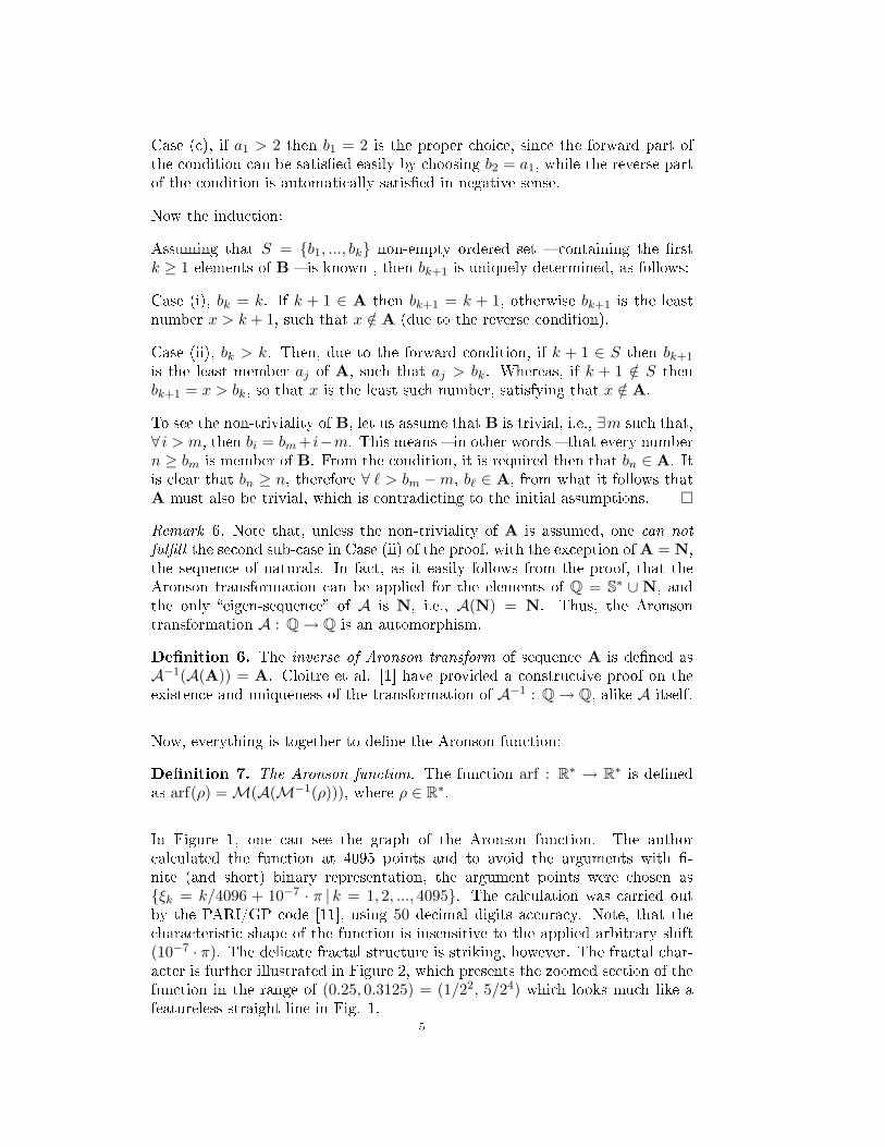
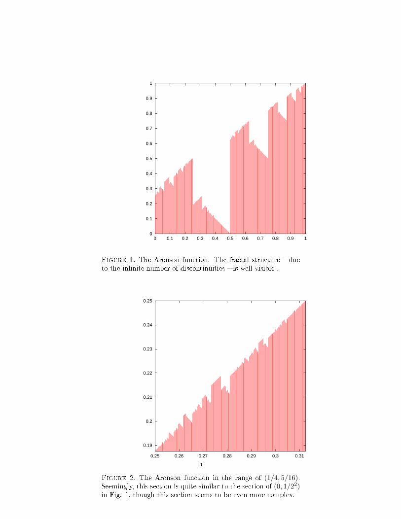
In Figure 1, one can see the graph of the Aronson function. The authorcalculated the function at 4095 points and to avoid the arguments with �-nite (and short) binary representation, the argument points were chosen as{ξk = k/4096 + 10−7 · π | k = 1, 2, ..., 4095}. The calculation was carried outby the PARI/GP code [11], using 50 decimal digits accuracy. Note, that thecharacteristic shape of the function is insensitive to the applied arbitrary shift(10−7 · π). The delicate fractal structure is striking, however. The fractal char-acter is further illustrated in Figure 2, which presents the zoomed section of thefunction in the range of (0.25, 0.3125) = (1/22, 5/24) which looks much like afeatureless straight line in Fig. 1.

5

0

0.1

0.2

0.3

0.4

0.5

0.6

0.7

0.8

0.9

1

0 0.1 0.2 0.3 0.4 0.5 0.6 0.7 0.8 0.9 1

Figure 1. The Aronson function. The fractal structure � dueto the in�nite number of discontinuities � is well visible .

0.19

0.2

0.21

0.22

0.23

0.24

0.25

0.25 0.26 0.27 0.28 0.29 0.3 0.31

Figure 2. The Aronson function in the range of (1/4, 5/16).Seemingly, this section is quite similar to the section of (0, 1/22)in Fig. 1, though this section seems to be even more complex.

6

Remark 7. By analyzing the Aronson function just by the naked eye, it looks likeconsisting of characteristic sections in the intervals: (0, 1/2), (1/2, 3/4), (3/4, 7/8), ....The general formula for the boundaries of the kth section is

(1)

(2k−1 − 1

2k−1,

2k − 12k

).

The shape of the function looks identical within these sections, apart from be-ing scaled to �t into the sections, i.e., scaled down by a factor of two at eachsubsequent intervals. This observation can easily be demonstrated to be true,since e.g., the sequences being isomorphic with the numbers in the second sec-tion, (1/2, 3/4) are almost the same as those corresponding to the �rst section(0, 1/2) with the only di�erence that all the sequences corresponding to the sec-ond section contain the number �1�, while none does it have in the �rst section(since no number in section one contains the �rst fractional binary digit). Sim-ilarly, the sequences corresponding to the numbers in the kth section start withthe �rst k − 1 consecutive natural numbers, since the corresponding numbersstart with k − 1 �1� digits. Thus, if a number in the kth section is at δ/2k dis-tance from the section`s starting point for some δ ∈ R∗, then the binary patternof that number starts with k − 1 digits of �1� , and then continues with thesame binary digit pattern as that of δ. In the domain of sequences this meansthat the corresponding sequence in the section k starts with the �rst k− 1 con-secutive naturals and then continues similarly to the sequence corresponding tothe number δ, with the only di�erence that the value of k − 1 is added to theevery member of the original sequence. In mathematical terms: if A =M−1(δ)for some δ ∈ R∗, and in the kth section A(k) =M−1

((2k−1 − 1)/2k−1 + δ/2k

),

then the term with index i > k of A(k) is

a(k)i = ai−k+1 + k − 1,

where ai−k+1 is the (i − k + 1)-th term of A. Hence, due to the features ofthe Aronson transformation (cf. with the proof of Theorem 2), the transform

of A(k)will also start with k − 1 binary digits of �1� and then will continueanalogously to the transform of A.

It is also notable that the co-domain corresponding to a section � as de�ned inequation (1) � in the domain of the Aronson function is identical to the domainsection itself. By scrutinizing the constructive proof of the Theorem 2, thisbehavior can be understood.

Clearly, by using the inverse Aronson transformation A−1 and the M binarymapping analogously to De�nition 7, a di�erent function can be obtained:

De�nition 8. The Aronson inverse function. The function arfi : R∗ → R∗ isde�ned as arfi(ρ) =M(A−1(M−1(ρ))), where ρ ∈ R∗.

Theorem 3. The inverse of the Aronson function is the Aronson inverse func-

tion: arfi(ρ) = arf−1(ρ).7

0

0.1

0.2

0.3

0.4

0.5

0.6

0.7

0.8

0.9

1

0 0.1 0.2 0.3 0.4 0.5 0.6 0.7 0.8 0.9 1

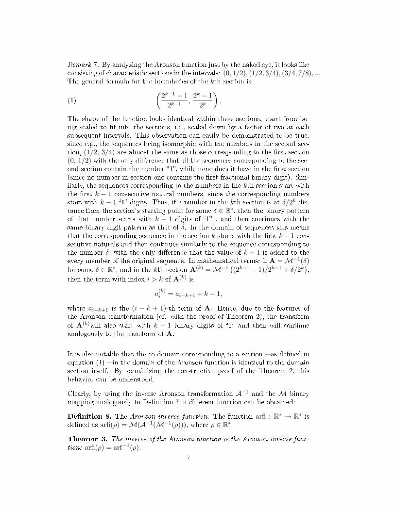
Figure 3. The Aronson function (arf) (continuous line) and theAronson inverse function (arf−1) (dashed line)(Note that the vertical lines are not parts of the functions!)

Proof. The claim follows from Theorem 2, since A(A) is an automorphism inS∗, therefore arf(ρ) = M(A(M−1(ρ))) is automorphism in R∗ and M is iso-morphism between S∗ and R∗.

More explicitely: in general, for f : X→ X automorphism the inverse f−1(x) ={x∗| f(x∗) = x} exists if x∗ ∈ X is unique and exists for every x ∈ X. Thus,arf−1(ρ) = {ρ∗| arf(ρ∗) = ρ}. Let denote the sequence M−1(ρ) = B and letassume that ρ∗ =M(A−1(B)). Then

arf(ρ∗) =M(A(M−1(ρ∗))) =M(A(M−1(M(A−1(B))))) =M(B) = ρ .

�

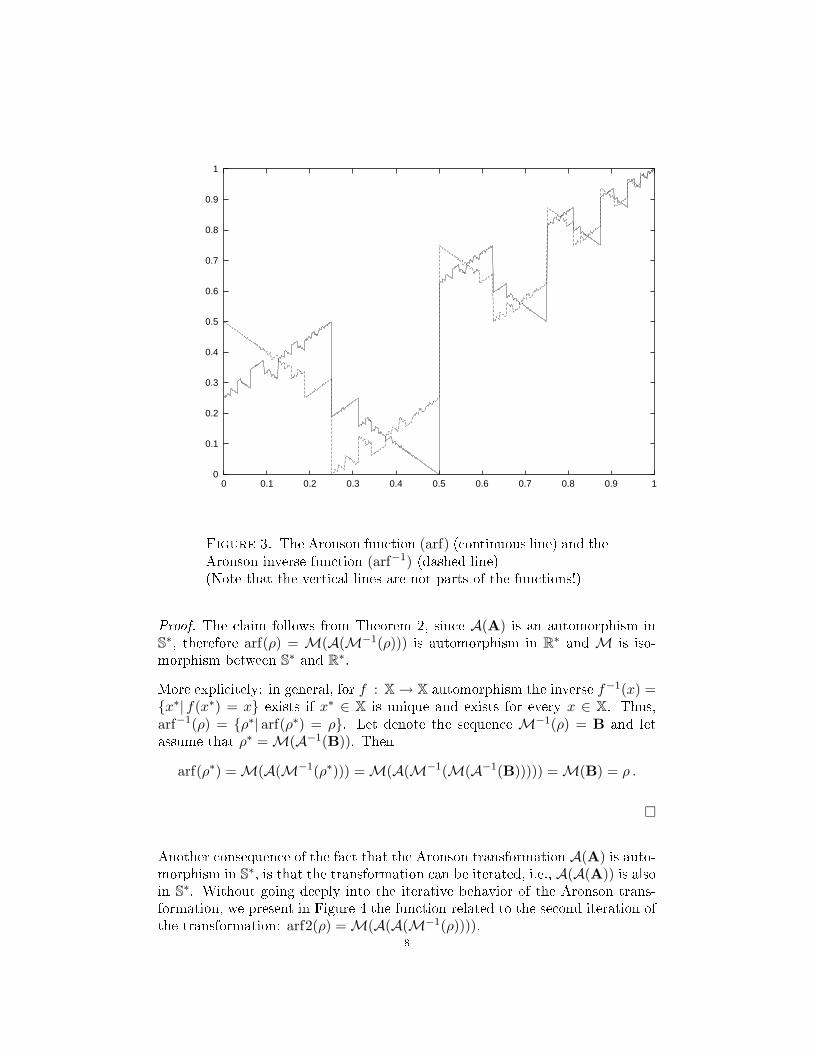
Another consequence of the fact that the Aronson transformation A(A) is auto-morphism in S∗, is that the transformation can be iterated, i.e., A(A(A)) is alsoin S∗. Without going deeply into the iterative behavior of the Aronson trans-formation, we present in Figure 4 the function related to the second iteration ofthe transformation: arf2(ρ) =M(A(A(M−1(ρ)))).

8

0

0.1

0.2

0.3

0.4

0.5

0.6

0.7

0.8

0.9

1

0 0.1 0.2 0.3 0.4 0.5 0.6 0.7 0.8 0.9 1

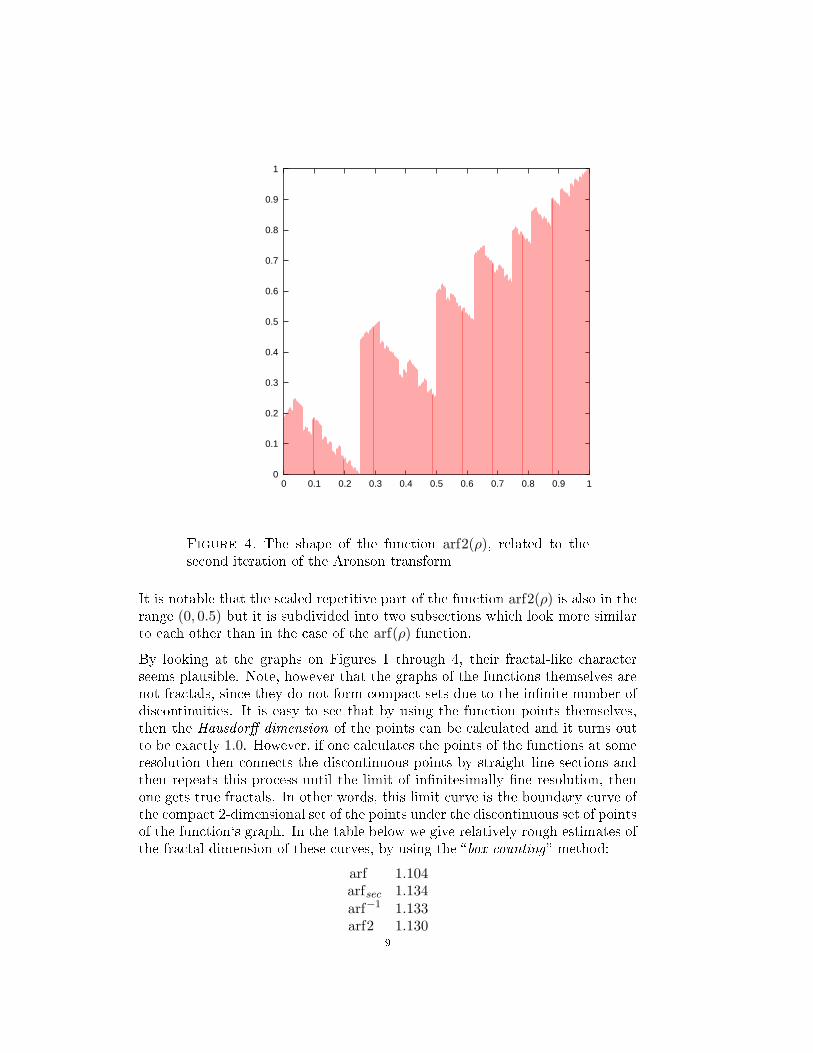
Figure 4. The shape of the function arf2(ρ), related to thesecond iteration of the Aronson transform

It is notable that the scaled repetitive part of the function arf2(ρ) is also in therange (0, 0.5) but it is subdivided into two subsections which look more similarto each other than in the case of the arf(ρ) function.

By looking at the graphs on Figures 1 through 4, their fractal-like characterseems plausible. Note, however that the graphs of the functions themselves arenot fractals, since they do not form compact sets due to the in�nite number ofdiscontinuities. It is easy to see that by using the function points themselves,then the Hausdor� dimension of the points can be calculated and it turns outto be exactly 1.0. However, if one calculates the points of the functions at someresolution then connects the discontinuous points by straight line sections andthen repeats this process until the limit of in�nitesimally �ne resolution, thenone gets true fractals. In other words, this limit curve is the boundary curve ofthe compact 2-dimensional set of the points under the discontinuous set of pointsof the function`s graph. In the table below we give relatively rough estimates ofthe fractal dimension of these curves, by using the �box counting� method:

arf 1.104arfsec 1.134arf−1 1.133arf2 1.130

9

where arfsec corresponds to the section of the arf function presented in Figure2, which � due to the �ner resolution � provided a somewhat higher value thenthe whole function. It can be seen that the fractal dimension of these curves israther similar, probably identical.

Remark. Without proving the Lebesgue integrability of arf, arf−1 and arf2 func-tions, computational evidence supports that their Lebesgue integral for the openinterval of (0, 1) is equal to 1/2.

4. Arithmetics with monotonic sequences

We have seen in Section 2 that the positive monotonic sequences are isomorphicto a subset of the real interval (0, 1), namely to R∗. Thus, for example thesequence of primes corresponds to the real number µ =M(P) (see A092856 in[3]):

0.41468250985111166024810962215430770836577423813791697786824541448864096...

what is quite close to√

2 − 1 but it is not identical. Also note that the realnumber above is identical to the real number created from the characteristicfunction of the sequence of primes (A010051 in [3]) as binary fractional digits.

Conversely, every irrational number in (0, 1) (and also many rationals) cor-responds to some monotonic integer sequence, e.g., M−1(

√2 − 1) yields the

sequence (A092855 in [3]):

2, 3, 5, 7, 13, 16, 17, 18, 19, 22, 23, 26, 27, 30, 31, 32, 33, 34, 35, 36, 39, 40, 41, 43, 44, 45,

46, 49, 50, 53, 56, 61, 65, 67, 68, 71, 73, 74, 75, 76, 77, 79, 80, 84, 87, 88, 90, 91, 94, 95, 97,

98, 99, 101, 103, 105, 108, 110, 112, 114, 115, 116, 117, 118, 120, 123, 124, 125, 126, 127, 131,

132, 133, 135, 137, 138, 140, 141, 142, 143, 145, 146, 152, 154, 155, 156, 158, 160, 164, 167,

170, 171, 172, 174, 175, 176, 178, 180, 185, 188, 189, 192, 193, 194, 196, 197, 199, 203, 205,

206, 207, 208, 210, 212, 213, 216, 221, 223, 224, 230, 231, 234, 235, 238, 239, 240, 243, 244,

247, 251, 253, 255... .

This sequence, alike a completely di�erent sequence, the Aronson transform ofthe �evil� sequence (A092863 in [3]), looks quite reach in primes. This peculiarityis deceiving, however in both cases, since by checking further the sequences, theexcess prime content vanishes.

Just one more example of mapping a mathematical constant into an integersequence is theM−1(1/

√2π) (A092857 in [3]):

2, 3, 6, 7, 11, 16, 20, 22, 25, 26, 29, 30, 31, 32, 34, 36, 41, 42, 44, 45, 48, 50, 55, 59, 60, 62, 67,

68, 69, 70, 71, 72, 75, 77, 78, 81, 82, 83, 84, 88, 90, 99, 101, 102, 103, 105, 107, 109, 110, 111,

115, 116, 117, 121, 123, 124, 125, 126, 127, 128,... .

Obviously, a sequence mapped from some mathematical constant may not bevery interesting, unless somebody �nds some known real constant γ, such thatM−1(γ) is an otherwise known sequence. Though the author made some e�ortsin this direction, they were unsuccessful, so far.

As it was mentioned in Section 2, an arithmetics of the sequences can be in-troduced corresponding to the arithmetics in its isomorphic map within the

10

interval (0, 1). Recalling: A ⊕B = M−1 (M(A)⊕M(B)) and also A ⊗B =M−1 (M(A) · M(B)).

Note that for the �addition�, as it is de�ned in De�nition 4, some restrictionsapply to make sure that the resulting set of integers is a �non-trivial� integersequence (cf. Def. 3). It is easy to see, that for two non-trivial sequences Aand B, A⊕B ∈ S∗, unless there is an index i in A and an index j in B, suchthat ∀ k > 0, ai+k = bj+k.

Thus, one can create e.g., the �sum� of the sequence of primesP and the sequenceof triangular numbers (A00217 in [3]) T, where ti = i(i+ 1)/2 (A092858 in [3]):

P⊕T =[5, 6, 7, 10, 11, 13, 15, 17, 19, 21, 23, 28, 29, 31, 36,...].

Similarly, the di�erence between T and P can also be given (A092859 in [3]):

T⊕P =[3, 4, 5, 7, 12, 13, 16, 18, 19, 22, 23, 30, 31, 38, 39, 40,...].

It is a direct consequence of having a de�ned addition that we can also multiplythe monotonic sequences by natural numbers. Obviously, 2P = P⊕P = X andthen xi = pi − 1. The sequence 3P (A092860 in [3]) is not so simple:

3P =[3, 4, 5, 6, 7, 10, 11, 12, 13, 16, 17, 18, 19, 22, 23, 28, 29, 30, 31, 36, 37,40, 41, 42, 43, 46, 47, 52, 53, 58, 59, 60, 61, 66, 67, 70, 71, 72, 73, 78, 79, 82,83, 88, 89, 96, 97,...],

in which sequence due to the truncation (fractional part of the sum) in De�nition1, one term is eliminated. Due to this e�ect, the inverse of integer multiplicationin general, does not exist.

As we have seen, the positive monotonic sequences form a semigroup over the�multiplication� as de�ned in Remark 3. The sequence A092861 in [3] illustratesthis:

P⊗E =[4, 7, 9, 12, 14, 15, 18, 19, 21, 25, 26, 33, 35, 36, 37, 40, 41, 42, 44, 47,48, 50, 54, 55, 58, 59, 60, 64, 65, 66, 69, 72, 77, 78, 79, 80, 84, 86, 87, 88, 89,90, 91, 97, 99, 100, 105, 106, 107, 108, 110, 111,...],

where E is the sequence of �evil numbers� (A001969 in [3]), containing thenumbers having even number of non-zero binary digits.

By having a well de�ned multiplication among the monotonic sequences, we alsocan create the integer powers of the sequences. Thus, for example, the squareof the prime sequence, P2 =M−1(M2(P)) (A092862 in [3]):

P2 =[3, 5, 6, 14, 16, 17, 19, 21, 22, 25, 27, 31, 32, 34, 36, 37, 41, 42, 44, 45, 48,49, 52, 54, 57, 59, 60, 62, 64, 65, 69, 74, 75, 78, 81, 88, 90, 91, 92, 94, 97, 98,100,...]

It is obvious, that this can be generalized for real exponents, as well. Thus, forexample, we can have the π as exponent for P (A092863 in [3]):

Pπ =[4, 7, 10, 16, 18, 20, 22, 23, 27, 28, 29, 31, 32, 33, 34, 35, 37, 38, 40, 42,46, 51, 57, 60, 65, 66, 67, 68, 69, 70, 72, 73, 74, 77, 78, 80, 81, 82, 84, 85, 89,91, 92, 93, 94, 95, 99, 101, 103, 107, 108, 110, 111, ...].

11

In general, it is easy to realize that for any function which is an automorphismin (0, 1), the inverse binary mapping de�nes uniquely an automorphic transfor-mation over the monotonic positive sequences.

5. Cellular Automaton Functions and Transformations

The cellular automata are known since the middle of the 20th century, thoughsystematic studies appeared only at the beginning of the 21st century, e.g., byIlachinski [10]. Also a very broad coverage of the topic � along with manyother types of recursive mappings � can be found in the book of S. Wolfram[9]. In that book (see p. 53) the individual one-dimensional cellular automata� where the next state of a cell is determined by itself and by its two neighbors� are identi�ed by 8-digit binary numbers (or an integer in the range of 0-255),where each of the digits determine the resulting state of the cell as function ofthe initial state of the 3 parent cells. For example the rule of the automatonidenti�ed by the number �30� is as follows:

111 110 101 100 011 010 001 0000 0 0 1 1 1 1 0 = 3010

.

This particular automaton � along with a few (13) others from among the pos-sible 255 di�erent kinds � exhibits a peculiar random-like behavior when it isapplied recursively, starting from a single cell. These kinds of automata arecategorized as �Class 3� and �Class 4� by S. Wolfram (p. 231 in [9]). Notethat about the half of all possible such automata are �trivial�, and many othersproduce regular, repetitive patterns.

De�nition 9. Cellular automaton mapping. Concerning a generic de�nition ofthe cellular automata, we refer to for example Ilachinski's book [10], but themost readily accessible resource is Eric W. Weisstein's MathWorld [2]. Here werestrict ourselves to the �one-dimensional, two-states, �rst neighbors� automata,which are also referred as elementary cellular automata in [2]. Let D denote anin�nite ordered set of discrete elements of two di�erent kinds (states): one ofthe kinds is identi�ed by �0� and the other by �1�. The ordering of the set D isone-dimensional, hence every member di has two neighbors: di−1 and di+1. LetD denote the set of such sets. The mapping C : D → D is a (one-dimensional,�rst-neighbors) cellular automaton maping if the member d′i of the image setD′ is determined from the members di−1, di, di+1 of D by applying the �rule�of the automaton, which uniquely de�nes the image value for every possiblecombination of the values di−1, di, di+1. Note that i ∈ (−∞,∞). Notaion:D′ =fC(D).

Remark 8. The de�nition above is applicable for �two-ways� in�nite orderedsets of binary digits � because this corresponds to the usual de�nitions �, butit is easily adaptable to ordered sets which are only �one-way� in�nite: i.e., formonotonic integer sequences. From among the three possible obvious ways, wehave chosen the one where d′i is determined by the set of di−2, di−1, di, alongwith postulating �0� values for the non-existent elements of d−1 and d0.

12

According to De�nition 1, we can map any monotonic sequence into an in�nitesequence of binary 1's and 0's. This suggests to introduce a transformation byapplying some cellular automaton such a way that after mapping the sequenceinto the form of a binary number, one applies the selected cellular automatonrule by shifting a 3-digit window over the binary digits of the number one-by-one, yielding the digits of the new number. Then, this new number is to bemapped back into the realm of integer sequences by using the inverse binary

mapping (De�nition 1).

De�nition 10. CA transformation of monotonic sequences. Due to the injec-tive character of binary mapping (as de�ned in Def. 1), any monotonic sequencecan be transformed according to any simple (and also other) cellular automatonC by the

CC(S) =M−1(fC(M(S)))formula, where fC(M(S)) is the cellural automaton mapping by using the au-tomaton C ofM(S), according to De�nition 9.

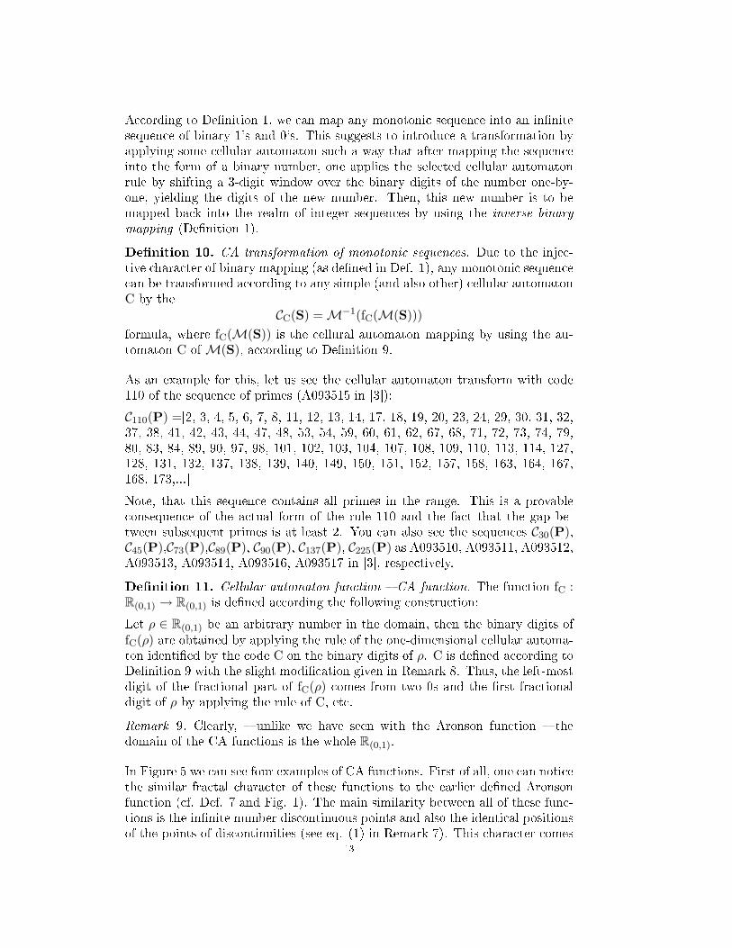
As an example for this, let us see the cellular automaton transform with code110 of the sequence of primes (A093515 in [3]):

C110(P) =[2, 3, 4, 5, 6, 7, 8, 11, 12, 13, 14, 17, 18, 19, 20, 23, 24, 29, 30, 31, 32,37, 38, 41, 42, 43, 44, 47, 48, 53, 54, 59, 60, 61, 62, 67, 68, 71, 72, 73, 74, 79,80, 83, 84, 89, 90, 97, 98, 101, 102, 103, 104, 107, 108, 109, 110, 113, 114, 127,128, 131, 132, 137, 138, 139, 140, 149, 150, 151, 152, 157, 158, 163, 164, 167,168, 173,...]

Note, that this sequence contains all primes in the range. This is a provableconsequence of the actual form of the rule 110 and the fact that the gap be-tween subsequent primes is at least 2. You can also see the sequences C30(P),C45(P),C73(P),C89(P), C90(P), C137(P), C225(P) as A093510, A093511, A093512,A093513, A093514, A093516, A093517 in [3], respectively.

De�nition 11. Cellular automaton function � CA function. The function fC :R(0,1) → R(0,1) is de�ned according the following construction:

Let ρ ∈ R(0,1) be an arbitrary number in the domain, then the binary digits offC(ρ) are obtained by applying the rule of the one-dimensional cellular automa-ton identi�ed by the code C on the binary digits of ρ. C is de�ned according toDe�nition 9 with the slight modi�cation given in Remark 8. Thus, the left-mostdigit of the fractional part of fC(ρ) comes from two 0s and the �rst fractionaldigit of ρ by applying the rule of C, etc.

Remark 9. Clearly, � unlike we have seen with the Aronson function � thedomain of the CA functions is the whole R(0,1).

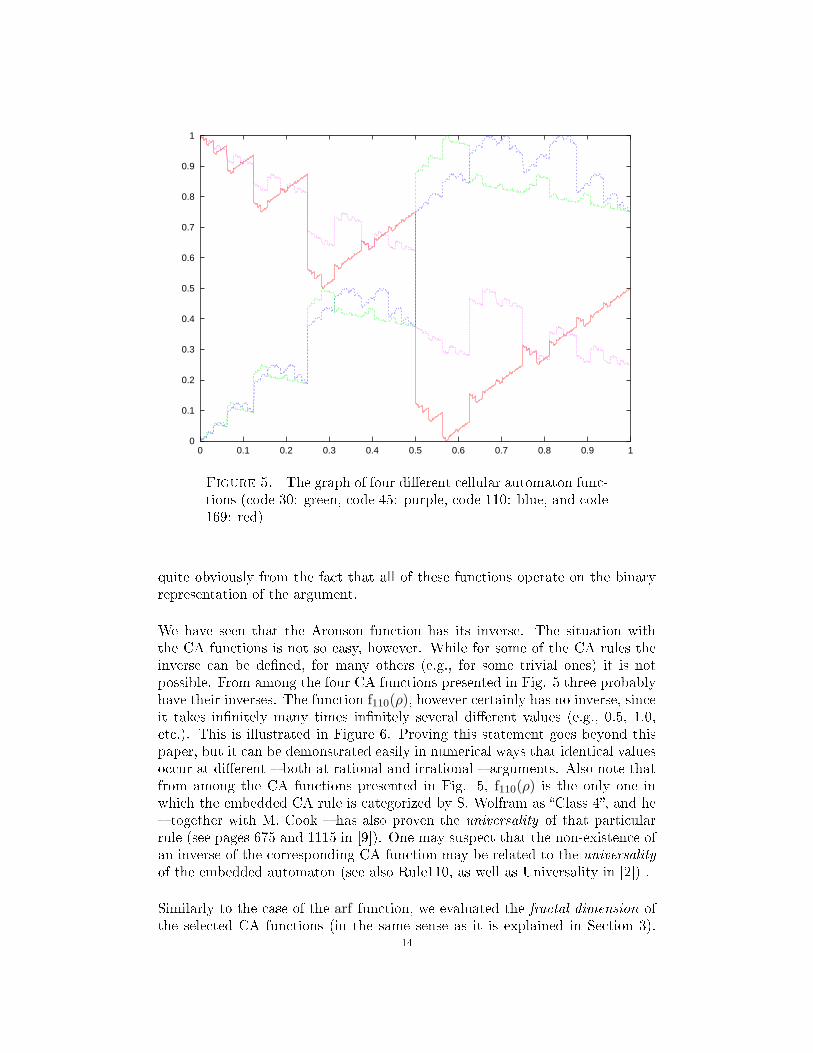
In Figure 5 we can see four examples of CA functions. First of all, one can noticethe similar fractal character of these functions to the earlier de�ned Aronsonfunction (cf. Def. 7 and Fig. 1). The main similarity between all of these func-tions is the in�nite number discontinuous points and also the identical positionsof the points of discontinuities (see eq. (1) in Remark 7). This character comes

13

0

0.1

0.2

0.3

0.4

0.5

0.6

0.7

0.8

0.9

1

0 0.1 0.2 0.3 0.4 0.5 0.6 0.7 0.8 0.9 1

Figure 5. The graph of four di�erent cellular automaton func-tions (code 30: green, code 45: purple, code 110: blue, and code169: red)

quite obviously from the fact that all of these functions operate on the binaryrepresentation of the argument.

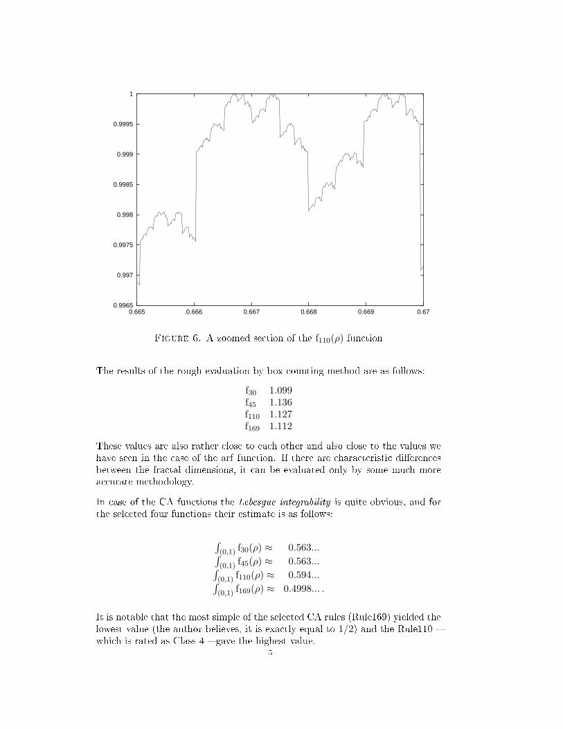
We have seen that the Aronson function has its inverse. The situation withthe CA functions is not so easy, however. While for some of the CA rules theinverse can be de�ned, for many others (e.g., for some trivial ones) it is notpossible. From among the four CA functions presented in Fig. 5 three probablyhave their inverses. The function f110(ρ), however certainly has no inverse, sinceit takes in�nitely many times in�nitely several di�erent values (e.g., 0.5, 1.0,etc.). This is illustrated in Figure 6. Proving this statement goes beyond thispaper, but it can be demonstrated easily in numerical ways that identical valuesoccur at di�erent � both at rational and irrational � arguments. Also note thatfrom among the CA functions presented in Fig. 5, f110(ρ) is the only one inwhich the embedded CA rule is categorized by S. Wolfram as �Class 4�, and he� together with M. Cook � has also proven the universality of that particularrule (see pages 675 and 1115 in [9]). One may suspect that the non-existence ofan inverse of the corresponding CA function may be related to the universalityof the embedded automaton (see also Rule110, as well as Universality in [2]) .

Similarly to the case of the arf function, we evaluated the fractal dimension ofthe selected CA functions (in the same sense as it is explained in Section 3).

14

0.9965

0.997

0.9975

0.998

0.9985

0.999

0.9995

1

0.665 0.666 0.667 0.668 0.669 0.67

Figure 6. A zoomed section of the f110(ρ) function

The results of the rough evaluation by box counting method are as follows:

f30 1.099f45 1.136f110 1.127f169 1.112

These values are also rather close to each other and also close to the values wehave seen in the case of the arf function. If there are characteristic di�erencesbetween the fractal dimensions, it can be evaluated only by some much moreaccurate methodology.

In case of the CA functions the Lebesgue integrability is quite obvious, and forthe selected four functions their estimate is as follows:

∫(0,1) f30(ρ) ≈ 0.563...∫(0,1) f45(ρ) ≈ 0.563...∫(0,1) f110(ρ) ≈ 0.594...∫(0,1) f169(ρ) ≈ 0.4998... .

It is notable that the most simple of the selected CA rules (Rule169) yielded thelowest value (the author believes, it is exactly equal to 1/2) and the Rule110 �which is rated as Class 4 � gave the highest value.

15

6. Conclusion

The isomorphism � named as binary mapping � as de�ned in De�nition 1 madepossible to map any monotonically increasing integer sequence to a real numberin (0, 1). Hence, having an automorphism over the monotonic sequences, weobtain a function with domain and codomain in (0, 1). Conversely, any auto-morphic function over (0, 1) corresponds to an automorphic transformation overthe set of monotonic sequences. The simple arithmetics de�ned between the se-quences potentially yields an immense number of new sequences and hopefullysome of them will exhibit important features. Perhaps, the isomorphism mayhelp exploring or even proving some peculiarities of some transformations of theinteger sequences, as well as some peculiarities of speci�c sequences.

The presented examples related to cellular automata provide new hints for con-tinuing the exploration of this relatively newly approached realm.

Acknowledgment

The author thanks Benoit Cloitre for his preliminary review, encouragementand valuable ideas.

Appendix:

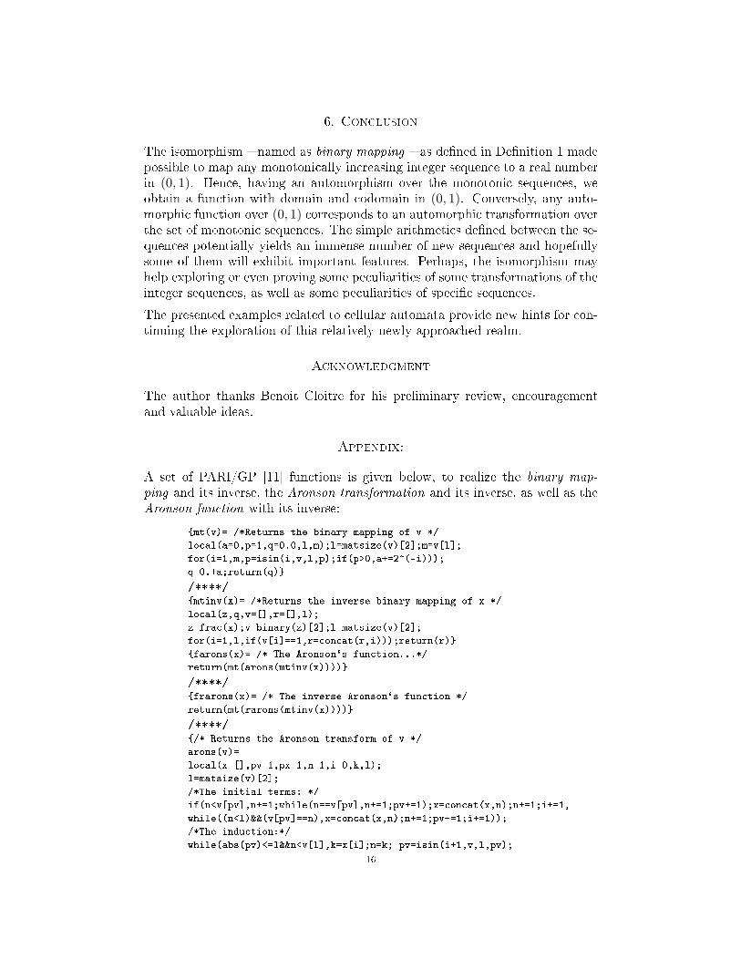
A set of PARI/GP [11] functions is given below, to realize the binary map-

ping and its inverse, the Aronson transformation and its inverse, as well as theAronson function with its inverse:

{mt(v)= /*Returns the binary mapping of v */

local(a=0,p=1,q=0.0,l,m);l=matsize(v)[2];m=v[l];

for(i=1,m,p=isin(i,v,l,p);if(p>0,a+=2^(-i)));

q=0.+a;return(q)}

/****/

{mtinv(x)= /*Returns the inverse binary mapping of x */

local(z,q,v=[],r=[],l);

z=frac(x);v=binary(z)[2];l=matsize(v)[2];

for(i=1,l,if(v[i]==1,r=concat(r,i)));return(r)}

{farons(x)= /* The Aronson`s function...*/

return(mt(arons(mtinv(x))))}

/****/

{frarons(x)= /* The inverse Aronson`s function */

return(mt(rarons(mtinv(x))))}

/****/

{/* Returns the Aronson transform of v */

arons(v)=

local(x=[],pv=1,px=1,n=1,i=0,k,l);

l=matsize(v)[2];

/*The initial terms: */

if(n<v[pv],n+=1;while(n==v[pv],n+=1;pv+=1);x=concat(x,n);n+=1;i+=1,

while((n<l)&&(v[pv]==n),x=concat(x,n);n+=1;pv+=1;i+=1));

/*The induction:*/

while(abs(pv)<=l&&n<v[l],k=x[i];n=k; pv=isin(i+1,v,l,pv);

16

/* pv>0 if (i+1) is in v */

if(k==i,n+=1;if(pv<0,pv=abs(pv); while(pv>0,n+=1; pv=isin(n,v,l,pv))),

px=isin(i+1,x,i,px); if(px>0,pv=-abs(pv);while(pv<0,n+=1;pv=isin(n,v,l,pv)),

pv=abs(pv);while(pv>0,n+=1;pv=isin(n,v,l,pv))));

x=concat(x,n);i+=1);/*print(i);*/ return(x) }

/****/

{ /* Returns the inverse Aronson transform of v */

rarons(v)=

local(h=[],c=[],x=[],pv=1,px=1,n=1,i,j=1,l,m=0,f);

l=matsize(v)[2];h=vector(l);c=vector(l);for(i=1,l,h[i]=[];c[i]=[]);

while(n<=l,while((n<v[j])&&(n<=l),c[n]=concat(c[n],v[n]);n+=1);

if(n<=l,h[n]=concat(h[n],v[n]);j+=1;n+=1));

n=1;while(n<=l,f=matsize(h[n])[2];

for(i=m+1,v[n]-1,if(f, c[n]=concat(c[n],i),

if((m<>n-1)||(i<>n), h[n]=concat(h[n],i), c[n]=concat(c[n],i)))); m=v[n];n+=1);

for(i=1,l,x=concat(x,h[i]));return(x) }

/****/

{isin(x,v,l,poi)=

/*If x integer is in v monotonic vector of length l,

the function returns a positive 'poi',

else a negative one. (�poi� is also used for acceleration,

the last returned value is recommended in the input) */

poi=abs(poi);if(poi==1&&x<v[1], return(-poi),

if(x<v[poi],while(x<v[poi]&&poi>1,poi-=1);

if(x<>v[poi],poi*=-1),

if(x>v[poi],while(x>v[poi]&&poi<l,poi+=1);

if(x<>v[poi],poi*=-1)));return(poi))}

References

[1] B. Cloitre, N. J. A. Sloane, M. J. Vandermast: Numerical analogues of Aronson's se-quence, J. Integer Seqs., Vol. 6 (2003), Art. 03.2.2,http://www.math.uwaterloo.ca/JIS/

[2] E. W. Weisstein et al.: Di�erent sections from MathWorld � A Wolfram Web Resource.http://mathworld.wolfram.com/CharacteristicFunction.html ,http://mathworld.wolfram.com/IversonBracket.html,http://mathworld.wolfram.com/Thue-MorseConstant.html,http://mathworld.wolfram.com/ElementaryCellularAutomaton.html,http://mathworld.wolfram.com/Rule30.htmlhttp://mathworld.wolfram.com/Rule110.htmlhttp://mathworld.wolfram.com/Universality.html

[3] N. J. A. Sloane, editor, 2004: The On-Line Encyclopedia of Integer Sequences,http://www.research.att.com/~njas/sequences/index.html

[4] J.-P. Allouche and J. Shallit, The ring of k-regular sequences, II, Theoret. Computer Sci.,307 (2003), 3-29.

[5] J.-P. Allouche and J. O. Shallit, The ubiquitous Prouhet-Thue-Morse sequence, in C.Ding. T. Helleseth and H. Niederreiter, eds., Sequences and Their Applications: Proceed-ings of SETA '98, Springer-Verlag, 1999, pp. 1-16.

[6] Ricardo Astudillo, On a class of Thue-Morse type sequences, J. Integer Seqs., Vol. 6,2003.http://www.math.uwaterloo.ca/JIS/

[7] J. K. Aronson, quoted by D. R. Hofstadter in Metamagical Themas [8], p. 44.[8] D. R. Hofstadter, Metamagical Themas, Basic Books, NY, 1985.[9] S. Wolfram, A New Kind of Science, Wolfram Media, 2002, ISBN I-57955-008-8

17

[10] A. Ilachinski, Cellular Automata, World Scienti�c, River Edge, MJ, 2001.[11] C. Batut et al.: User's guide to PARI/GP,

http://www.parigp-home.de and also ftp://megrez.math.u-bordeaux.fr/pub/pari

18