Beyond Junction Trees: Loopy Graphical Modelsjebara/6772/notes/notes10old.pdf · Loopy Belief...
59
Beyond Junction Trees: Loopy Graphical Models Tony Jebara April 16, 2013
Transcript of Beyond Junction Trees: Loopy Graphical Modelsjebara/6772/notes/notes10old.pdf · Loopy Belief...

Beyond Junction Trees: Loopy Graphical Models
Tony Jebara
April 16, 2013
Graphical Models
x1 x2 x3 x4
x5
x6
Figure: p(X ) = 1Zψ1,2(x1, x2)ψ2,3(x2, x3)ψ3,4,5(x3, x4, x5)ψ4,5,6(x4, x5, x6).
Key for efficient inference, learning, structured prediction
A compact way of representing p(X ) = p(x1, . . . , xk)
We want p(xi ) =∑
X\xip(X ) or x∗
i where p(X ∗) ≥ p(X )
Factor graph: a more precise way to specify an undirectedgraphical model
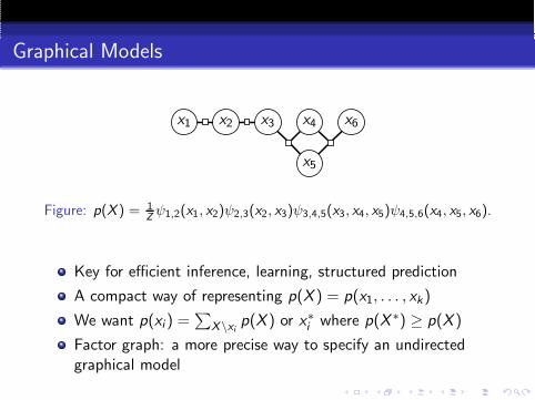
Factor Graphs
x1 x2 x3 x4
x5
x6
Figure: p(X ) = 1Zψ1,2(x1, x2)ψ2,3(x2, x3)ψ3,4,5(x3, x4, x5)ψ4,5,6(x4, x5, x6).
A bipartite graph G with variable vertices V = 1, . . . , k,factor vertices W = 1, . . . , l and edges E between V and E
With a universe of discrete random variables X = x1, . . . , xkeach associated with an element of V
With a set of strictly positive potential functionsΨ = ψ1, . . . , ψl each associated with an element of W
Factor graph represents p(x1, . . . , xk) = 1Z
∏
c∈W ψc (Xc)where Xc are variables associated with neighbors of c
Junction Tree Algorithm
Given a graphical model representing p(X ) = p(x1, . . . , xk)
Junction Tree Algorithm exactly finds p(xi) or x∗i via:
MoralizeTriangulateConnect cliques into junction tree (Kruskal)Send messages via Collect and Distribute
Caveat: messages are exponential in clique size
Problem: triangulation create giant cliques in many graphicalmodels and structured prediction problems!
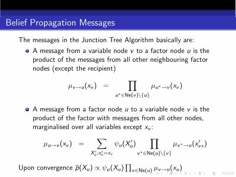
Belief Propagation Messages
The messages in the Junction Tree Algorithm basically are:
A message from a variable node v to a factor node u is theproduct of the messages from all other neighbouring factornodes (except the recipient)
µv→u(xv ) =∏
u∗∈Ne(v)\u
µu∗→v (xv )
A message from a factor node u to a variable node v is theproduct of the factor with messages from all other nodes,marginalised over all variables except xv :
µu→v(xv ) =∑
X ′u :x ′
v=xv
ψu(X′u)
∏
v∗∈Ne(u)\v
µv∗→u(x′v∗)
Upon convergence p(Xu) ∝ ψu(Xu)∏
v∈Ne(u) µv→u(xu)

Loopy Belief Propagation
These messages lead to exact inference for trees!
To get ArgMax junction tree, replace sum with max
What happens if we skip triangulation and don’t have a tree?
We can still run and hope for the best!
This is called loopy belief propagation
Used in turbo coding, image processing, protein folding, etc.
It works remarkably well in many experiments!
We can also prove it will work... on PERFECT GRAPHS!
This includes trees, matchings, associative graphical models
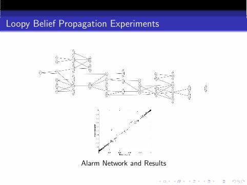
Loopy Belief Propagation Experiments
Alarm Network and Results
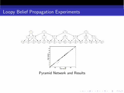
Loopy Belief Propagation Experiments
Pyramid Network and Results
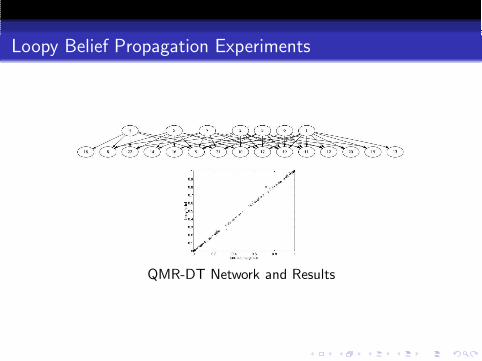
Loopy Belief Propagation Experiments
QMR-DT Network and Results
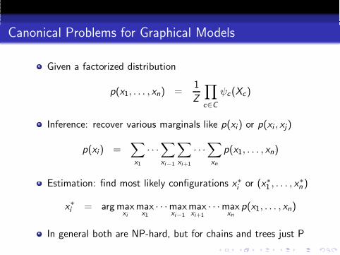
Canonical Problems for Graphical Models
Given a factorized distribution
p(x1, . . . , xn) =1
Z
∏
c∈C
ψc(Xc)
Inference: recover various marginals like p(xi) or p(xi , xj)
p(xi) =∑
x1
· · ·∑
xi−1
∑
xi+1
· · ·∑
xn
p(x1, . . . , xn)
Estimation: find most likely configurations x∗i or (x∗
1 , . . . , x∗n )
x∗i = arg max
xi
maxx1
· · ·maxxi−1
maxxi+1
· · ·maxxn
p(x1, . . . , xn)
In general both are NP-hard, but for chains and trees just P
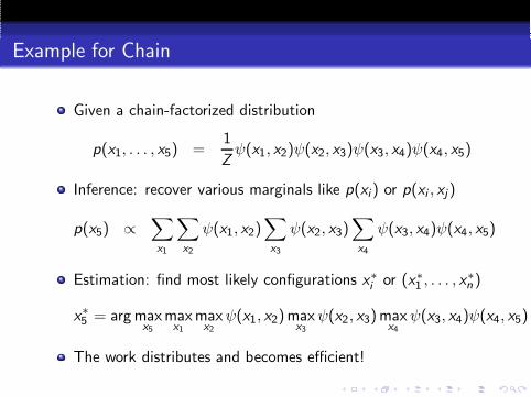
Example for Chain
Given a chain-factorized distribution
p(x1, . . . , x5) =1
Zψ(x1, x2)ψ(x2, x3)ψ(x3, x4)ψ(x4, x5)
Inference: recover various marginals like p(xi) or p(xi , xj)
p(x5) ∝∑
x1
∑
x2
ψ(x1, x2)∑
x3
ψ(x2, x3)∑
x4
ψ(x3, x4)ψ(x4, x5)
Estimation: find most likely configurations x∗i or (x∗
1 , . . . , x∗n )
x∗5 = arg max
x5
maxx1
maxx2
ψ(x1, x2)maxx3
ψ(x2, x3)maxx4
ψ(x3, x4)ψ(x4, x5)
The work distributes and becomes efficient!
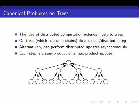
Canonical Problems on Trees
The idea of distributed computation extends nicely to trees
On trees (which subsume chains) do a collect/distribute step
Alternatively, can perform distributed updates asynchronously
Each step is a sum-product or a max-product update

Canonical Problems on Trees
The idea of distributed computation extends nicely to trees
On trees (which subsume chains) do a collect/distribute step
Alternatively, can perform distributed updates asynchronously
Each step is a sum-product or a max-product update

MAP Estimation
Let’s focus on finding most probable configurations efficiently
X ∗ = arg max p(x1, . . . , xn)
Useful for image processing, protein folding, coding, etc.
Brute force requires∏n
i=1 |xi |Efficient for trees and singly linked graphs (Pearl 1988)
NP-hard for general graphs (Shimony 1994)

Loopy Max Product Message Passing
1. For each xi to each Xc : mt+1i→c =
∏
d∈Ne(i)\c mtd→i
2. For each Xc to each xi : mt+1c→i = maxXc\xi
ψc(Xc)∏
j∈c\i mtj→c
3. Set t = t + 1 and goto 1 until convergence4. Output x∗
i = arg maxxi
∏
d∈Ne(i) mtd→i
Simple and fast algorithm for MAP
Performs well in practice for images, turbo codes, etc.
Exact for trees (Pearl 1988)
Exact for matching (Bayati et al. 2005)
Exact for generalized b matching (Huang and J 2007)
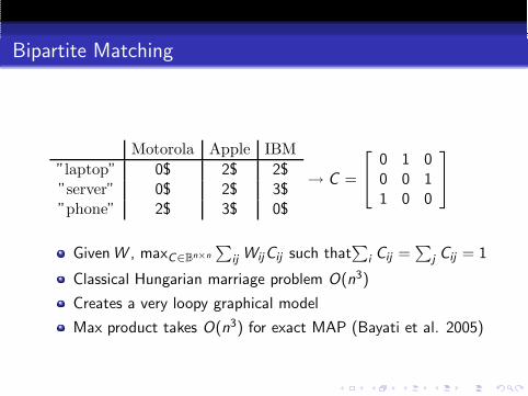
Bipartite Matching
Motorola Apple IBM
”laptop” 0$ 2$ 2$”server” 0$ 2$ 3$”phone” 2$ 3$ 0$
→ C =
0 1 00 0 11 0 0
GivenW , maxC∈Bn×n
∑
ij WijCij such that∑
i Cij =∑
j Cij = 1
Classical Hungarian marriage problem O(n3)
Creates a very loopy graphical model
Max product takes O(n3) for exact MAP (Bayati et al. 2005)
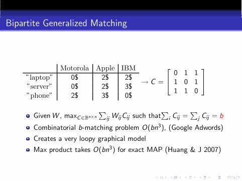
Bipartite Generalized Matching
Motorola Apple IBM
”laptop” 0$ 2$ 2$”server” 0$ 2$ 3$”phone” 2$ 3$ 0$
→ C =
0 1 11 0 11 1 0
GivenW , maxC∈Bn×n
∑
ij WijCij such that∑
i Cij =∑
j Cij = b
Combinatorial b-matching problem O(bn3), (Google Adwords)
Creates a very loopy graphical model
Max product takes O(bn3) for exact MAP (Huang & J 2007)
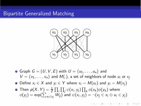
Bipartite Generalized Matching
u1 u2 u3 u4
v1 v2 v3 v4
Graph G = (U,V ,E ) with U = u1, . . . , un andV = v1, . . . , vn and M(.), a set of neighbors of node ui or vj
Define xi ∈ X and yi ∈ Y where xi = M(ui ) and yi = M(vj)
Then p(X ,Y ) = 1Z
∏
i
∏
j ψ(xi , yj )∏
k φ(xk)φ(yk) whereφ(yj ) = exp(
∑
ui∈yjWij) and ψ(xi , yj ) = ¬(vj ∈ xi ⊕ ui ∈ yj)
Bipartite Generalized Matching
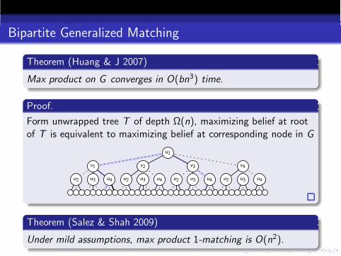
Theorem (Huang & J 2007)
Max product on G converges in O(bn3) time.
Proof.
Form unwrapped tree T of depth Ω(n), maximizing belief at rootof T is equivalent to maximizing belief at corresponding node in G
u1
v1 v2 v3 v4
u2 u2 u2 u2u3 u3 u3 u3u4 u4 u4 u4
Theorem (Salez & Shah 2009)
Under mild assumptions, max product 1-matching is O(n2).

Bipartite Generalized Matching
Code at http://www.cs.columbia.edu/∼jebara/code
Generalized Matching
2040
50100
0
0.05
0.1
0.15
b
BP median running time
n
t
2040
50100
0
50
100
150
b
GOBLIN median running time
n
t
20 40 60 80 1000
1
2
3
n
t1/3
Median Running time when B=5
20 40 60 80 1000
1
2
3
4
n
t1/4
Median Running time when B= n/2
BPGOBLIN
BPGOBLIN
Applications:unipartite matchingclustering (J & S 2006)classification (H & J 2007)collaborative filtering (H & J 2008)semisupervised (J et al. 2009)visualization (S & J 2009)
Max product is O(n2) on dense graphs (Salez & Shah 2009)Much faster than other solvers
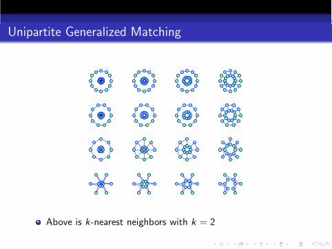
Unipartite Generalized Matching
Above is k-nearest neighbors with k = 2
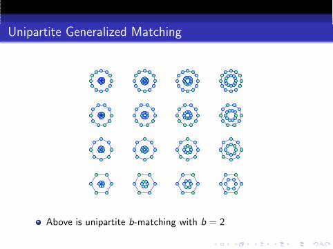
Unipartite Generalized Matching
Above is unipartite b-matching with b = 2
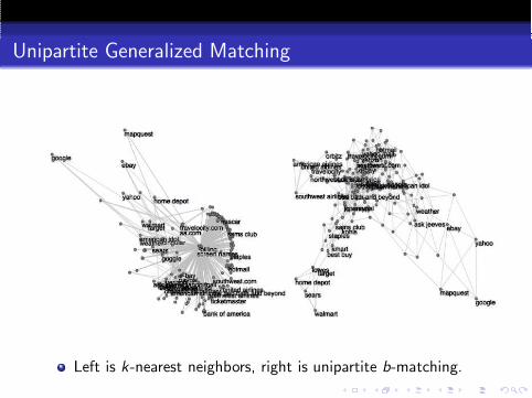
Unipartite Generalized Matching
Left is k-nearest neighbors, right is unipartite b-matching.
Unipartite Generalized Matching
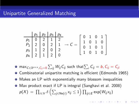
p1 p2 p3 p4
p1 0 2 1 2P2 2 0 2 1p3 1 2 0 2p4 2 1 2 0
→ C =
0 1 0 11 0 1 00 1 0 11 0 1 0
maxC∈Bn×n,Cii=0
∑
ij WijCij such that∑
i Cij = b,Cij = Cji
Combinatorial unipartite matching is efficient (Edmonds 1965)
Makes an LP with exponentially many blossom inequalities
Max product exact if LP is integral (Sanghavi et al. 2008)
p(X ) =∏
i∈V δ(
∑
j∈Ne(i) xij ≤ 1)
∏
ij∈E exp(Wijxij)
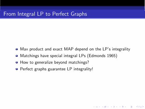
From Integral LP to Perfect Graphs
Max product and exact MAP depend on the LP’s integrality
Matchings have special integral LPs (Edmonds 1965)
How to generalize beyond matchings?
Perfect graphs guarantee LP integrality!

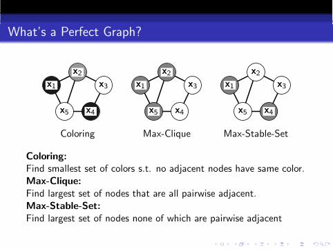
What’s a Perfect Graph?
In 1960, Claude Berge introduces perfect graphs and twoconjectures
Perfect iff every induced subgraph has clique # = coloring #
Weak conjecture: G is perfect iff its complement is perfectStrong conjecture: all perfect graphs are Berge graphs
Weak perfect graph theorem (Lovasz 1972)
Link between perfection and integral LPs (Lovasz 1972)
Strong perfect graph theorem (SPGT) open for 4+ decades

What’s a Perfect Graph?
SPGT Proof (Chudnovsky, Robertson, Seymour, Thomas 2003)
Berge passes away shortly after hearing of the proof
Many NP-hard problems are polynomially solvable for perfectgraphs:
Graph coloringMaximum cliqueMaximum independent set
What’s a Perfect Graph?
x1
x2
x3
x4x5
x1
x2
x3
x4x5
x1
x2
x3
x4x5
Coloring Max-Clique Max-Stable-Set
Coloring:
Find smallest set of colors s.t. no adjacent nodes have same color.Max-Clique:
Find largest set of nodes that are all pairwise adjacent.Max-Stable-Set:
Find largest set of nodes none of which are pairwise adjacent
What’s a Perfect Graph?
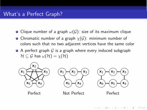
Clique number of a graph ω(G): size of its maximum clique
Chromatic number of a graph χ(G): minimum number ofcolors such that no two adjacent vertices have the same color
A perfect graph G is a graph where every induced subgraphH ⊆ G has ω(H) = χ(H)
x1
x2
x3
x4x5
x1 x2 x3
x4x5
x1 x2 x3
x4x5x6
Perfect Not Perfect Perfect
Strong Perfect Graph Theorem
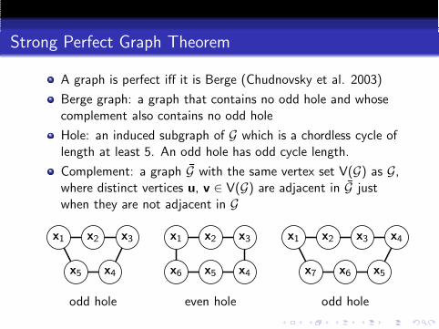
A graph is perfect iff it is Berge (Chudnovsky et al. 2003)
Berge graph: a graph that contains no odd hole and whosecomplement also contains no odd hole
Hole: an induced subgraph of G which is a chordless cycle oflength at least 5. An odd hole has odd cycle length.
Complement: a graph G with the same vertex set V(G) as G,where distinct vertices u, v ∈ V(G) are adjacent in G justwhen they are not adjacent in G
x1 x2 x3
x4x5
x1 x2 x3
x4x5x6
x1 x2 x3 x4
x5x6x7
odd hole even hole odd hole

Strong Perfect Graph Theorem
SPGT implies that a Berge graph is one of these primitives
bipartite graphscomplements of bipartite graphsline graphs of bipartite graphscomplements of line graphs of bipartite graphsdouble split graphs
or decomposes structurally (into graph primitives)
via a 2-joinvia a 2-join in the complementvia an M-joinvia a balanced skew partition
Line graph: L(G) a graph which contains a vertex for eachedge of G and where two vertices of L(G) are adjacent iff theycorrespond to two edges of G with a common end vertex
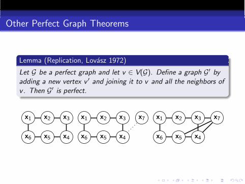
Other Perfect Graph Theorems
Lemma (Replication, Lovasz 1972)
Let G be a perfect graph and let v ∈ V(G). Define a graph G′ byadding a new vertex v ′ and joining it to v and all the neighbors ofv . Then G′ is perfect.
x1 x2 x3
x4x5x6
x1 x2 x3
x4x5x6
x7 x1 x2 x3
x4x5x6
x7
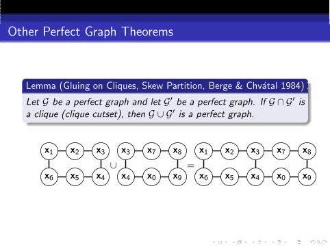
Other Perfect Graph Theorems
Lemma (Gluing on Cliques, Skew Partition, Berge & Chvatal 1984)
Let G be a perfect graph and let G′ be a perfect graph. If G ∩ G′ isa clique (clique cutset), then G ∪ G′ is a perfect graph.
x1 x2 x3
x4x5x6
∪x3 x7 x8
x9x0x4
=
x1 x2 x3
x4x5x6
x7 x8
x9x0
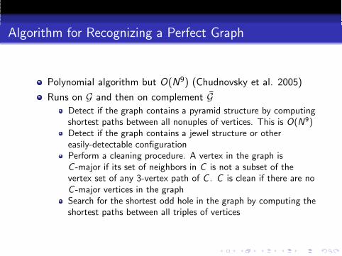
Algorithm for Recognizing a Perfect Graph
Polynomial algorithm but O(N9) (Chudnovsky et al. 2005)
Runs on G and then on complement GDetect if the graph contains a pyramid structure by computingshortest paths between all nonuples of vertices. This is O(N9)Detect if the graph contains a jewel structure or othereasily-detectable configurationPerform a cleaning procedure. A vertex in the graph isC -major if its set of neighbors in C is not a subset of thevertex set of any 3-vertex path of C . C is clean if there are noC -major vertices in the graphSearch for the shortest odd hole in the graph by computing theshortest paths between all triples of vertices

Integral Linear Programming with Perfect Graphs
Max product and exact MAP depend on the LP’s integrality
Matchings have special integral LPs (Edmonds 1965)
How to generalize beyond matchings?
Perfect graphs imply LP integrality (Lovasz 1972)
Lemma (Lovasz 1972)
For every non-negative vector ~f ∈ RN , the linear program
β = max~x∈RN
~f ⊤~x subject to ~x ≥ 0 and A~x ≤ ~1
recovers a vector ~x which is integral if and only if the(undominated) rows of A form the vertex versus maximal cliquesincidence matrix of some perfect graph.
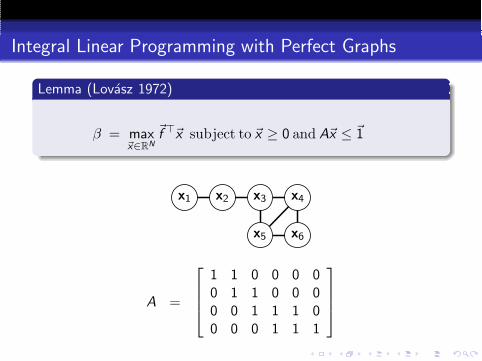
Integral Linear Programming with Perfect Graphs
Lemma (Lovasz 1972)
β = max~x∈RN
~f ⊤~x subject to ~x ≥ 0 and A~x ≤ ~1
x1 x2 x3 x4
x5 x6
A =
1 1 0 0 0 00 1 1 0 0 00 0 1 1 1 00 0 0 1 1 1
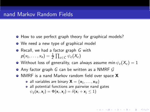
nand Markov Random Fields
How to use perfect graph theory for graphical models?
We need a new type of graphical model
Recall, we had a factor graph G withp(x1, . . . , xn) = 1
Z
∏
c∈C ψc (Xc)
Without loss of generality, can always assume minψc(Xc) = 1
Any factor graph G can be written as a NMRF GNMRF is a nand Markov random field over space X
all variables are binary X = x1, . . . , xNall potential functions are pairwise nand gatesψij(xi , xj) = Φ(xi , xj) = δ(xi + xj ≤ 1)
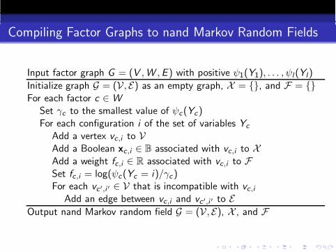
Compiling Factor Graphs to nand Markov Random Fields
Input factor graph G = (V ,W ,E ) with positive ψ1(Y1), . . . , ψl (Yl)
Initialize graph G = (V, E) as an empty graph, X = , and F = For each factor c ∈ W
Set γc to the smallest value of ψc(Yc)For each configuration i of the set of variables Yc
Add a vertex vc,i to VAdd a Boolean xc,i ∈ B associated with vc,i to XAdd a weight fc,i ∈ R associated with vc,i to FSet fc,i = log(ψc(Yc = i)/γc )For each vc′,i ′ ∈ V that is incompatible with vc,i
Add an edge between vc,i and vc′,i ′ to EOutput nand Markov random field G = (V, E), X , and F
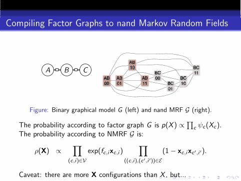
Compiling Factor Graphs to nand Markov Random Fields
A B CAB
00
AB
01
AB
10
AB
11
BC
00
BC
01
BC
10
BC
11
Figure: Binary graphical model G (left) and nand MRF G (right).
The probability according to factor graph G is p(X ) ∝ ∏
c ψc(Xc).The probability according to NMRF G is:
ρ(X) ∝∏
(c,i)∈V
exp(fc,ixc,i )∏
((c,i),(c′ ,i ′))∈E
(1 − xc,ixc′,i ′).
Caveat: there are more X configurations than X , but...
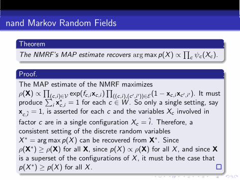
nand Markov Random Fields
Theorem
The NMRF’s MAP estimate recovers arg max p(X ) ∝ ∏
c ψc(Xc).
Proof.
The MAP estimate of the NMRF maximizesρ(X) ∝ ∏
(c,i)∈V exp(fc,ixc,i )∏
((c,i),(c′ ,i ′))∈E (1 − xc,ixc′,i ′). It mustproduce
∑
i x∗c,i = 1 for each c ∈ W . So only a single setting, say
xc ,i
= 1, is asserted for each c and the variables Xc involved in
factor c are in a single configuration Xc = i . Therefore, aconsistent setting of the discrete random variablesX ∗ = arg max p(X ) can be recovered from X∗. Sinceρ(X∗) ≥ ρ(X) for all X, since p(X ) ∝ ρ(X) for all X , and since X
is a superset of the configurations of X , it must be the case thatp(X ∗) ≥ p(X ) for all X .

nand Markov Random Fields
How do we find the MAP estimate for the NMRF?
It can be solved simply by finding the maximal stable set!
More precisely solve a maximal maximum weight stable set(MMWSS) problem.
These are polynomial time if the graph is perfect.
Definition (Maximal Maximum Weight Stable Set)
The maximal maximum weight stable set of a graph G = (V, E)with non-negative weights F is a maximum weight stable set of Gwith largest cardinality.
nand Markov Random Fields
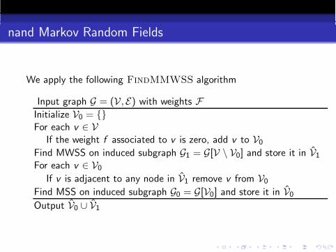
We apply the following FindMMWSS algorithm
Input graph G = (V, E) with weights FInitialize V0 = For each v ∈ V
If the weight f associated to v is zero, add v to V0
Find MWSS on induced subgraph G1 = G[V \ V0] and store it in V1
For each v ∈ V0
If v is adjacent to any node in V1 remove v from V0
Find MSS on induced subgraph G0 = G[V0] and store it in V0
Output V0 ∪ V1

Solving MWSS in Practice
Three ways to solve the MWSS problem on a perfect graph:
Linear programming
Message passing
Semidefinite programming

MWSS via Linear Programming
maxx∈Rn,x≥0
f⊤x s.t. Ax ≤ 1 (1)
This is known as a set-packing linear program
A ∈ Rm×n is vertex versus maximal cliques incidence matrix
If graph G is perfect, LP is binary and solves MWSS
Run-time is O(√
mn3) where m is number of cliques in graph
Problem: m = |C| can be exponential in n...
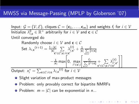
MWSS via Message-Passing (MPLP by Globerson ’07)
Input: G = (V, E), cliques C = c1, . . . , cm and weights fi for i ∈ VInitialize λ0
i ,c ∈ R+ arbitrarily for i ∈ V and c ∈ C
Until converged doRandomly choose i ∈ V and c ∈ CSet λi ,c
(t+1) = 1−|c||c|
∑
c′∈C\c:i∈c′λ
(t)i ,c′ + 1
|c|fi
P
c∈C
[i∈c]
− 1|c| max
[
0, maxi ′∈c\i
[
fi′P
c∈C
[i ′∈c] +∑
c′∈C\c:i ′∈c′λ
(t)i ′,c′
]]
Output: x∗i =
∑
c∈C:i∈c λi ,c(t) for i ∈ V
Slight variation of max-product messages
Problem: only provably correct for bipartite NMRFs
Problem: m = |C| can be exponential in n...
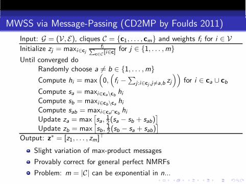
MWSS via Message-Passing (CD2MP by Foulds 2011)
Input: G = (V, E), cliques C = c1, . . . , cm and weights fi for i ∈ VInitialize zj = maxi∈cj
fiP
c∈C[i∈c] for j ∈ 1, . . . ,m
Until converged doRandomly choose a 6= b ∈ 1, . . . ,mCompute hi = max
(
0,(
fi −∑
j :i∈cj ,j 6=a,b zj
))
for i ∈ ca ∪ cb
Compute sa = maxi∈ca\cbhi
Compute sb = maxi∈cb\cahi
Compute sab = maxi∈ca∩cbhi
Update za = max[
sa,12(sa − sb + sab)
]
Update zb = max[
sb,12(sb − sa + sab)
]
Output: z∗ = [z1, . . . , zm]⊤
Slight variation of max-product messages
Provably correct for general perfect NMRFs
Problem: m = |C| can be exponential in n...
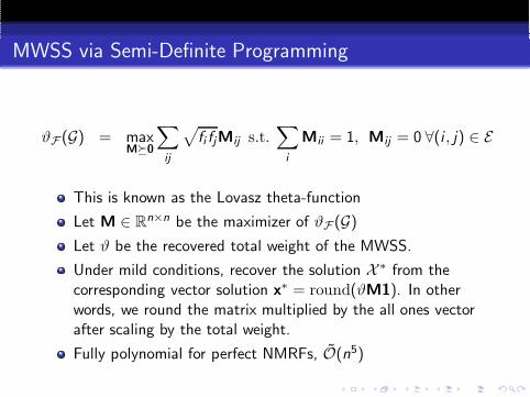
MWSS via Semi-Definite Programming
ϑF (G) = maxM0
∑
ij
√
fi fjMij s.t.∑
i
Mii = 1, Mij = 0 ∀(i , j) ∈ E
This is known as the Lovasz theta-function
Let M ∈ Rn×n be the maximizer of ϑF (G)
Let ϑ be the recovered total weight of the MWSS.
Under mild conditions, recover the solution X ∗ from thecorresponding vector solution x∗ = round(ϑM1). In otherwords, we round the matrix multiplied by the all ones vectorafter scaling by the total weight.
Fully polynomial for perfect NMRFs, O(n5)
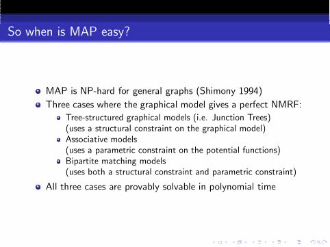
So when is MAP easy?
MAP is NP-hard for general graphs (Shimony 1994)
Three cases where the graphical model gives a perfect NMRF:
Tree-structured graphical models (i.e. Junction Trees)(uses a structural constraint on the graphical model)Associative models(uses a parametric constraint on the potential functions)Bipartite matching models(uses both a structural constraint and parametric constraint)
All three cases are provably solvable in polynomial time
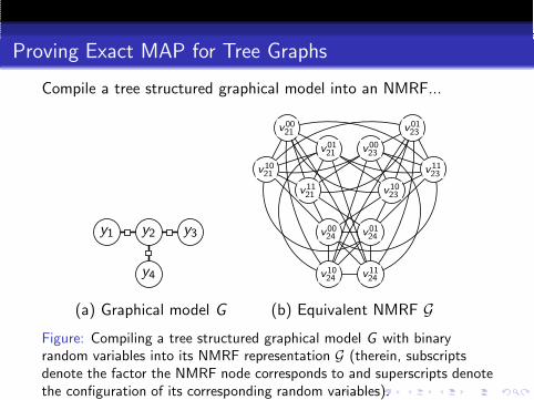
Proving Exact MAP for Tree Graphs
Compile a tree structured graphical model into an NMRF...
y1 y2 y3
y4
v0021
v0121
v1021
v1121
v0023
v0123
v1023
v1123
v0024 v01
24
v1024 v11
24
(a) Graphical model G (b) Equivalent NMRF GFigure: Compiling a tree structured graphical model G with binaryrandom variables into its NMRF representation G (therein, subscriptsdenote the factor the NMRF node corresponds to and superscripts denotethe configuration of its corresponding random variables).
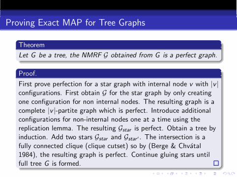
Proving Exact MAP for Tree Graphs
Theorem
Let G be a tree, the NMRF G obtained from G is a perfect graph.
Proof.
First prove perfection for a star graph with internal node v with |v |configurations. First obtain G for the star graph by only creatingone configuration for non internal nodes. The resulting graph is acomplete |v |-partite graph which is perfect. Introduce additionalconfigurations for non-internal nodes one at a time using thereplication lemma. The resulting Gstar is perfect. Obtain a tree byinduction. Add two stars Gstar and Gstar ′ . The intersection is afully connected clique (clique cutset) so by (Berge & Chvatal1984), the resulting graph is perfect. Continue gluing stars untilfull tree G is formed.
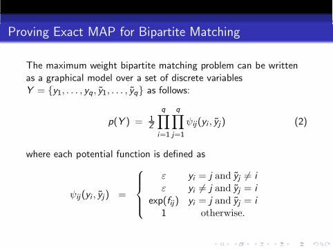
Proving Exact MAP for Bipartite Matching
The maximum weight bipartite matching problem can be writtenas a graphical model over a set of discrete variablesY = y1, . . . , yq, y1, . . . , yq as follows:
p(Y ) = 1Z
q∏
i=1
q∏
j=1
ψij(yi , yj ) (2)
where each potential function is defined as
ψij (yi , yj ) =
ε yi = j and yj 6= iε yi 6= j and yj = i
exp(fij) yi = j and yj = i1 otherwise.
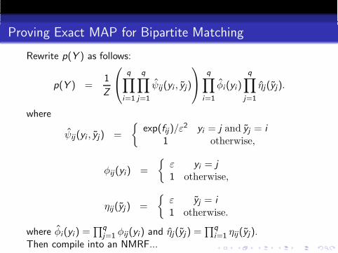
Proving Exact MAP for Bipartite Matching
Rewrite p(Y ) as follows:
p(Y ) =1
Z
q∏
i=1
q∏
j=1
ψij(yi , yj)
q∏
i=1
φi (yi )
q∏
j=1
ηj(yj).
where
ψij(yi , yj) =
exp(fij)/ε2 yi = j and yj = i
1 otherwise,
φij(yi) =
ε yi = j1 otherwise,
ηij(yj ) =
ε yj = i1 otherwise.
where φi (yi ) =∏q
j=1 φij(yi ) and ηj(yj ) =∏q
i=1 ηij(yj).Then compile into an NMRF...
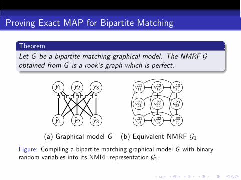
Proving Exact MAP for Bipartite Matching
Theorem
Let G be a bipartite matching graphical model. The NMRF Gobtained from G is a rook’s graph which is perfect.
y1 y2 y3
y1 y2 y3 v3131 v32
32 v3333
v2121 v22
22 v2323
v1111 v12
12 v1313
(a) Graphical model G (b) Equivalent NMRF G1
Figure: Compiling a bipartite matching graphical model G with binaryrandom variables into its NMRF representation G1.
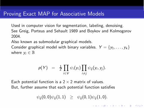
Proving Exact MAP for Associative Models
Used in computer vision for segmentation, labeling, denoising.See Greig, Porteus and Sehault 1989 and Boykov and Kolmogorov2004.Also known as submodular graphical models.Consider graphical model with binary variables. Y = y1, . . . , ykwhere yi ∈ B
p(Y ) = 1Z
∏
i∈V
ψi (yi )∏
i 6=j
ψij (yi , yj ).
Each potential function is a 2 × 2 matrix of values.But, further assume that each potential function satisfies
ψij(0, 0)ψij (1, 1) ≥ ψij(0, 1)ψij (1, 0).
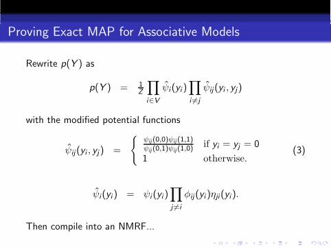
Proving Exact MAP for Associative Models
Rewrite p(Y ) as
p(Y ) = 1Z
∏
i∈V
ψi(yi )∏
i 6=j
ψij(yi , yj)
with the modified potential functions
ψij(yi , yj) =
ψij (0,0)ψij (1,1)ψij (0,1)ψij (1,0)
if yi = yj = 0
1 otherwise.(3)
ψi(yi ) = ψi (yi )∏
j 6=i
φij(yi )ηji(yi ).
Then compile into an NMRF...
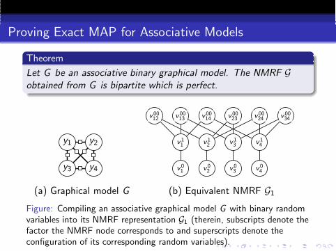
Proving Exact MAP for Associative Models
Theorem
Let G be an associative binary graphical model. The NMRF Gobtained from G is bipartite which is perfect.
y1 y2
y3 y4
v0012 v00
13 v0014 v00
23 v0024 v00
34
v01 v0
2 v03 v0
4
v11 v1
2 v13 v1
4
(a) Graphical model G (b) Equivalent NMRF G1
Figure: Compiling an associative graphical model G with binary randomvariables into its NMRF representation G1 (therein, subscripts denote thefactor the NMRF node corresponds to and superscripts denote theconfiguration of its corresponding random variables).
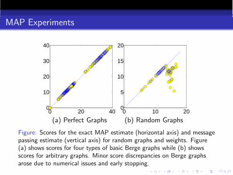
MAP Experiments
0 20 400
10
20
30
40
0 10 200
5
10
15
20
(a) Perfect Graphs (b) Random Graphs
Figure: Scores for the exact MAP estimate (horizontal axis) and messagepassing estimate (vertical axis) for random graphs and weights. Figure(a) shows scores for four types of basic Berge graphs while (b) showsscores for arbitrary graphs. Minor score discrepancies on Berge graphsarose due to numerical issues and early stopping.
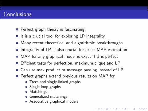
Conclusions
Perfect graph theory is fascinating
It is a crucial tool for exploring LP integrality
Many recent theoretical and algorithmic breakthroughs
Integrality of LP is also crucial for exact MAP estimation
MAP for any graphical model is exact if G is perfect
Efficient tests for perfection, maximum clique and LP
Can use max product or message passing instead of LP
Perfect graphs extend previous results on MAP for
Trees and singly-linked graphsSingle loop graphsMatchingsGeneralized matchingsAssociative graphical models


![Gamma Radiation-Induced Disruption of Cellular Junctions ...downloads.hindawi.com/journals/omcl/2019/1486232.pdf · junction protein [13]. Connexins compose the gap junction channels](https://static.fdocument.org/doc/165x107/5f06b4cd7e708231d4195458/gamma-radiation-induced-disruption-of-cellular-junctions-junction-protein-13.jpg)