Bergman Kernel and K¨ahler Tensor Calculushaoxu/paper/KahlerTensor.pdfWe will use the Einstein...
40
Pure and Applied Mathematics Quarterly Volume 9, Number 3 507—546, 2013 Bergman Kernel and K¨ ahler Tensor Calculus Hao Xu Abstract: Fefferman [22] initiated a program of expressing the asymptotic expansion of the boundary singularity of the Bergman kernel for strictly pseudoconvex domains explicitly in terms of boundary invariants. Hirachi, Komatsu and Nakazawa [30] carried out computations of the first few terms of Fefferman’s asymptotic expansion building partly on Graham’s work on CR invariants and Nakazawa’s work on the asymptotic expansion of the Bergman kernel for strictly pseudoconvex complete Reinhardt domains. In this paper, we prove a formula for coefficients in Nakazawa’s asymptotic expansion as explicit summations over strongly connected graphs, and a formula expressing partial derivatives of K¨ ahler metrics (resp. functions) as summations over rooted trees encoding covariant derivatives of curvature tensors (resp. functions). These formulae shall be useful in studying general patterns of Fefferman’s asymptotic expansion. Keywords: Bergman kernel, asymptotic expansion, Laplace integral. 1. Introduction The heat kernel on Riemannian manifolds plays an important role in index theory, general relativity and cosmology. A central object of study is the short- time expansion of the heat kernel of the Laplacian operator, K(t,x,x) ∼ ∞ j =0 a j (x)t j −d/2 ,t → 0+, where d is the manifold’s dimension and the coefficients a j (x) are invariant poly- nomials of jets of metrics. By H. Weyl’s work on the invariants of the orthogonal Received August 21, 2012.
Transcript of Bergman Kernel and K¨ahler Tensor Calculushaoxu/paper/KahlerTensor.pdfWe will use the Einstein...
Pure and Applied Mathematics Quarterly
Volume 9, Number 3
507—546, 2013
Bergman Kernel and Kahler Tensor Calculus
Hao Xu
Abstract: Fefferman [22] initiated a program of expressing the asymptotic
expansion of the boundary singularity of the Bergman kernel for strictly
pseudoconvex domains explicitly in terms of boundary invariants. Hirachi,
Komatsu and Nakazawa [30] carried out computations of the first few terms
of Fefferman’s asymptotic expansion building partly on Graham’s work on
CR invariants and Nakazawa’s work on the asymptotic expansion of the
Bergman kernel for strictly pseudoconvex complete Reinhardt domains. In
this paper, we prove a formula for coefficients in Nakazawa’s asymptotic
expansion as explicit summations over strongly connected graphs, and a
formula expressing partial derivatives of Kahler metrics (resp. functions)
as summations over rooted trees encoding covariant derivatives of curvature
tensors (resp. functions). These formulae shall be useful in studying general
patterns of Fefferman’s asymptotic expansion.
Keywords: Bergman kernel, asymptotic expansion, Laplace integral.
1. Introduction
The heat kernel on Riemannian manifolds plays an important role in index
theory, general relativity and cosmology. A central object of study is the short-
time expansion of the heat kernel of the Laplacian operator,
K(t, x, x) ∼
∞∑
j=0
aj(x)tj−d/2, t→ 0+,
where d is the manifold’s dimension and the coefficients aj(x) are invariant poly-
nomials of jets of metrics. By H. Weyl’s work on the invariants of the orthogonal
Received August 21, 2012.
508 Hao Xu
group, any invariant polynomial can be formed from Riemannian curvature ten-
sor by covariant differentiations, multiplications and contractions. It is a very
difficult problem to put a tensor expressions into a canonical form on a gen-
eral Riemmanian manifold. While the asymptotic expansion of the heat kernel
has important applications in spectral geometry (see [58] for a recent survey), it
seems hopeless to detect any meaningful structure of its combinatorially explosive
coefficients.
The ubiquitousness of heat kernels can be seen most clearly in Liu’s work
[39, 40, 41], where the heat kernel was used as a unifying tool to solve problems
in algebra, geometry and topology.
Let Ω be a (bounded) domain in Cn and A2(Ω) the Bergman space of holo-
morphic functions in L2(Ω). The (unweighted) Bergman kernel of Ω is a real
analytic function given by K(z) =∑
j |φj(z)|2 for z ∈ Ω, where φj is an ar-
bitrary orthonormal basis of A2(Ω). In [22], Fefferman initiated a program of
studying the Bergman kernel of a strictly pseudoconvex domain as an analogy of
the heat kernel, with the time variable t replaced by a defining function of the
domain. Fefferman’s program opened up the subject [3, 25, 27, 30] and has been
extended to conformal geometry; a major recent breakthrough is Alexakis’ proof
[1] of the Deser-Schwimmer conjecture.
Yau [55, p.679] proposed to classify pseudoconvex domains whose Bergman
metrics are Kahler-Einstein. A conjecture of S.-Y. Cheng says that if the Bergman
metric of a strictly pseudoconvex domain is Kahler-Einstein, then the domain is
biholomorphic to the ball (cf. [23]). The deep works of Cheng-Yau [11] and Mok-
Yau [47] showed that on a bounded domain of holomorphy, there exists a unique
biholomorphic invariant complete Kahler-Einstein metric with scalar curvature
−1.
The complete asymptotic expansion of the weighted Bergman kernel has been
established by Englis [18] for bounded strictly pseudoconvex domains in Cn with
real analytic boundary. For compact Kahler manifolds, in the 1980’s, Yau [56,
p.139] initiated the program of approximating Kahler-Einstein metrics by em-
beddings into complex projective space by higher power sections of an ample
holomorphic line bundle. The corresponding complete asymptotic expansion of
Bergman kernels was established independently by Zelditch [57] and Catlin [9],
which has important applications in the study of extremal metrics [15, 56]. It
Bergman Kernel and Kahler Tensor Calculus 509
can be viewed as the local version of the Hirzebruch-Riemann-Roch theorem.
Thanks to the Kahler condition dω = 0, the space of Weyl invariant polynomi-
als on Kahler manifolds has a canonical basis represented by multi-digraphs. A
closed formula has been discovered [51] for coefficients in the asymptotic expan-
sion of the weighted Bergman kernel. We expect that a similar formula should
exist for the heat kernel of the Laplacian operator on Kahler manifolds.
Karabegov and Schlichenmaier [35] showed that the logarithm of the diagonal
value of the weighted Bergman kernel is the Karabegov classifying form of the
Berezin quantization. There has been much work on deformation quantization of
Kahler manifolds and its applications (see the recent survey [50]).
We summarize the definitions and properties of curvature tensors on Kahler
manifolds. Let (M,g) be a Kahler manifold of dimension n. Locally the Kahler
form is given by ωg =√−12π
∑ni,j=1 gijdzi∧dzj . We will use the Einstein summation
convention. The indices i, j, k, . . . run from 1 to n, while Greek indices α, β, γ
may represent either i or i. Let det g be the determinant of the Hermitian matrix
(gij) and (gij) be the inverse of the matrix (gij). We also use the notations
gjkα1α2...αm:= ∂α1α2...αmgjk, fα1α2...αm := ∂α1α2...αmf,
(Rijkl/α1···αm)β1···βr
:= ∂β1···βrRijkl/α1···αm
.
The curvature tensor is defined as
(1) Rijkl = −gijkl + gmpgmjlgipk.
The Ricci tensor is given by Rij = gklRijkl = −∂i∂j log(det g) and the trace of
the Ricci curvature is the scalar curvature ρ = gijRij .
The covariant derivative of a covariant tensor field Tβ1...βpis defined by
(2) Tβ1...βp/γ = ∂γTβ1...βp−
p∑
i=1
ΓδγβiTβ1...βi−1δβi+1...βp
,
where the Christoffel symbols Γαβγ = 0 except for Γi
jk = gilgjlk, Γijk
= gligljk.
Lemma 1.1. On Kahler manifolds, we have ∂igjk = ∂jgik, ∂lgjk = ∂kgjl and
∂αgml = −gplgmqgpqα, ∂α det g = det g · gmlgmlα,(3)
Rijkl = Rilkj = Rkjil (first Bianchi),(4)
Rijkl/m = Rmjkl/i = Rijml/k, Rijkl/p = Ripkl/j = Rijkp/l (second Bianchi)(5)
510 Hao Xu
Tβ1...βp/ij − Tβ1...βp/ji = 0, Tβ1...βp/ij − Tβ1...βp/ji = 0,(6)
Tβ1...βp/ij − Tβ1...βp/ji =
p∑
k=1
Rγβkij
Tβ1...βk−1γβk+1...βp(Ricci formula),(7)
where Rklij
= −gmkRmlij, Rklij
= gkmRlmij and Rklij
= Rklij
= 0.
Recall that around each point x on a Kahler manifold M , there exists a normal
coordinate system such that gij(x) = δij , gijk1...kr(x) = gijl1...lr(x) = 0 for all
r ≤ N ∈ N, where N can be chosen arbitrary large.
Fix a normal coordinate system around x on M . By (1) and (2), it is not
difficult to see inductively that for any partial derivatives of metrics or curvature
tensors, there exists a canonical tensor that coincides with it at x. We will use
the operator D to denote this correspondence. For example, D(gijkl) = −Rijkl,
D(gijklα) = −Rijkl/α and
(8) D((Rijkl/p1···pm
)q1···qr
)= Rijkl/p1···pmq1···qr
.
As shown in [51, 52], tensor calculus on Kahler manifolds could be naturally
formulated in terms of graphs. In particular, the Weyl invariants [22] can be
represented by multi-digraphs. Each vertex in the graph is a partial derivatives
of metrics in local coordinates. Note such graphs are not in one-to-one corre-
spondence with tensorial vertices due to the Ricci formula.
In §2, we review Fefferman’s program, especially the works of [25, 30]. More
detailed and nice expositions can be found in [29]. In §3, building on work
of Englis [17], we prove a graph-theoretic formula for Nakazawa’s asymptotic
expansion. In §4-§6, we will prove closed formulae for the above operator D
as a summation over rooted trees with external legs, by canonically associate a
tensor expression to each rooted tree. As an illustration of the efficiency of these
formulae, we rederive the weight 3 coefficient in the asymptotic expansion of the
weighted Bergman kernel.
Acknowledgements The author thanks Professors Kefeng Liu and Shing-Tung
Yau for helpful conversations and encouragements. The author also thanks Pro-
fessors Miroslav Englis and Kengo Hirachi for helpful communications, whose
influence on this paper is evident.
Bergman Kernel and Kahler Tensor Calculus 511
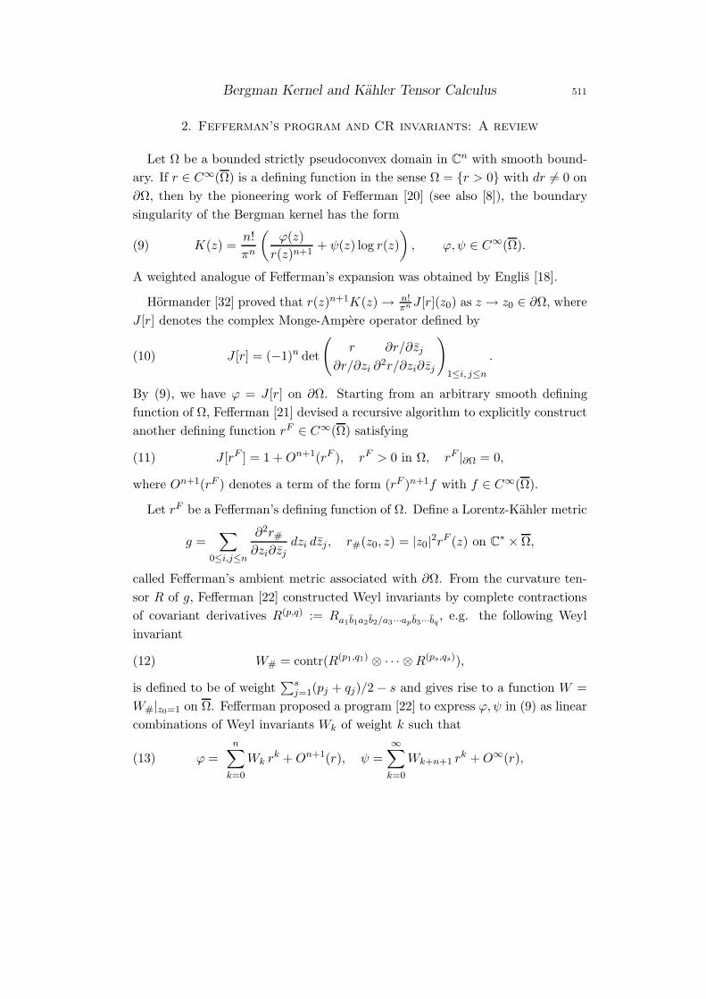
2. Fefferman’s program and CR invariants: A review
Let Ω be a bounded strictly pseudoconvex domain in Cn with smooth bound-
ary. If r ∈ C∞(Ω) is a defining function in the sense Ω = r > 0 with dr 6= 0 on
∂Ω, then by the pioneering work of Fefferman [20] (see also [8]), the boundary
singularity of the Bergman kernel has the form
(9) K(z) =n!
πn
(ϕ(z)
r(z)n+1+ ψ(z) log r(z)
), ϕ, ψ ∈ C∞(Ω).
A weighted analogue of Fefferman’s expansion was obtained by Englis [18].
Hormander [32] proved that r(z)n+1K(z) → n!πnJ [r](z0) as z → z0 ∈ ∂Ω, where
J [r] denotes the complex Monge-Ampere operator defined by
(10) J [r] = (−1)n det
(r ∂r/∂zj
∂r/∂zi ∂2r/∂zi∂zj
)
1≤i, j≤n
.
By (9), we have ϕ = J [r] on ∂Ω. Starting from an arbitrary smooth defining
function of Ω, Fefferman [21] devised a recursive algorithm to explicitly construct
another defining function rF ∈ C∞(Ω) satisfying
(11) J [rF ] = 1 +On+1(rF ), rF > 0 in Ω, rF |∂Ω = 0,
where On+1(rF ) denotes a term of the form (rF )n+1f with f ∈ C∞(Ω).
Let rF be a Fefferman’s defining function of Ω. Define a Lorentz-Kahler metric
g =∑
0≤i,j≤n
∂2r#∂zi∂zj
dzi dzj , r#(z0, z) = |z0|2rF (z) on C
∗ × Ω,
called Fefferman’s ambient metric associated with ∂Ω. From the curvature ten-
sor R of g, Fefferman [22] constructed Weyl invariants by complete contractions
of covariant derivatives R(p,q) := Ra1 b1a2 b2/a3···ap b3···bq, e.g. the following Weyl
invariant
(12) W# = contr(R(p1,q1) ⊗ · · · ⊗R(ps,qs)),
is defined to be of weight∑s
j=1(pj + qj)/2 − s and gives rise to a function W =
W#|z0=1 on Ω. Fefferman proposed a program [22] to express ϕ,ψ in (9) as linear
combinations of Weyl invariants Wk of weight k such that
(13) ϕ =n∑
k=0
Wk rk +On+1(r), ψ =
∞∑
k=0
Wk+n+1 rk +O∞(r),
512 Hao Xu
where O∞(r) means that ψ =∑m
k=0Wk+n+1[r] rk + Om+1(r) for any m ≥ 0.
The expansion of ϕ was proved by Fefferman [22] and Bailey et al. [3] for any
Fefferman’s defining function r = rF . The expansion of ψ was proved by Hirachi
[27] for more refined defining functions than (11). Both are very deep works.
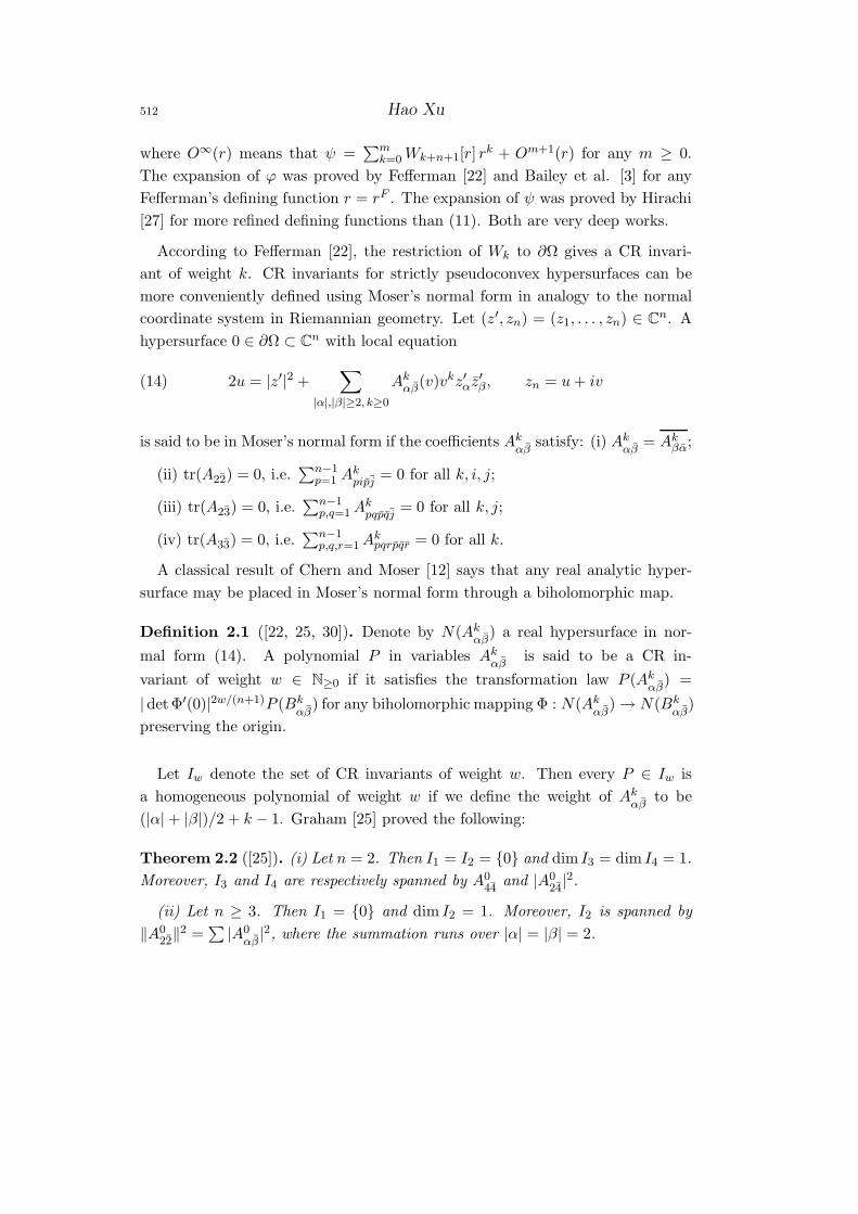
According to Fefferman [22], the restriction of Wk to ∂Ω gives a CR invari-
ant of weight k. CR invariants for strictly pseudoconvex hypersurfaces can be
more conveniently defined using Moser’s normal form in analogy to the normal
coordinate system in Riemannian geometry. Let (z′, zn) = (z1, . . . , zn) ∈ Cn. A
hypersurface 0 ∈ ∂Ω ⊂ Cn with local equation
(14) 2u = |z′|2 +∑
|α|,|β|≥2, k≥0
Akαβ(v)vkz′αz
′β, zn = u+ iv
is said to be in Moser’s normal form if the coefficients Akαβ
satisfy: (i) Akαβ
= Akβα;
(ii) tr(A22) = 0, i.e.∑n−1
p=1 Akpipj
= 0 for all k, i, j;
(iii) tr(A23) = 0, i.e.∑n−1
p,q=1Akpqpqj
= 0 for all k, j;
(iv) tr(A33) = 0, i.e.∑n−1
p,q,r=1Akpqrpqr = 0 for all k.
A classical result of Chern and Moser [12] says that any real analytic hyper-
surface may be placed in Moser’s normal form through a biholomorphic map.
Definition 2.1 ([22, 25, 30]). Denote by N(Akαβ
) a real hypersurface in nor-
mal form (14). A polynomial P in variables Akαβ
is said to be a CR in-
variant of weight w ∈ N≥0 if it satisfies the transformation law P (Akαβ
) =
|detΦ′(0)|2w/(n+1)P (Bkαβ
) for any biholomorphic mapping Φ : N(Akαβ
) → N(Bkαβ
)
preserving the origin.
Let Iw denote the set of CR invariants of weight w. Then every P ∈ Iw is
a homogeneous polynomial of weight w if we define the weight of Akαβ
to be
(|α| + |β|)/2 + k − 1. Graham [25] proved the following:
Theorem 2.2 ([25]). (i) Let n = 2. Then I1 = I2 = 0 and dim I3 = dim I4 = 1.
Moreover, I3 and I4 are respectively spanned by A044
and |A024|2.
(ii) Let n ≥ 3. Then I1 = 0 and dim I2 = 1. Moreover, I2 is spanned by
‖A022‖
2 =∑
|A0αβ
|2, where the summation runs over |α| = |β| = 2.
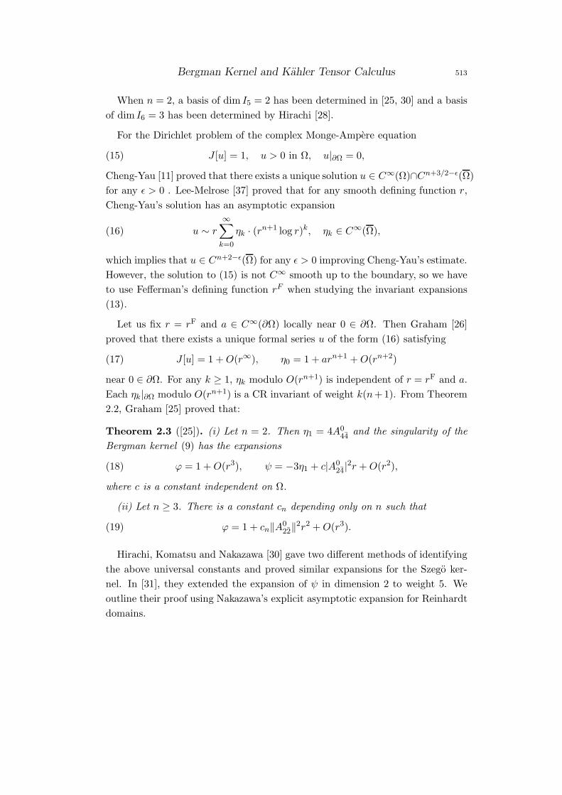
Bergman Kernel and Kahler Tensor Calculus 513
When n = 2, a basis of dim I5 = 2 has been determined in [25, 30] and a basis
of dim I6 = 3 has been determined by Hirachi [28].
For the Dirichlet problem of the complex Monge-Ampere equation
(15) J [u] = 1, u > 0 in Ω, u|∂Ω = 0,
Cheng-Yau [11] proved that there exists a unique solution u ∈ C∞(Ω)∩Cn+3/2−ǫ(Ω)
for any ǫ > 0 . Lee-Melrose [37] proved that for any smooth defining function r,
Cheng-Yau’s solution has an asymptotic expansion
(16) u ∼ r
∞∑
k=0
ηk · (rn+1 log r)k, ηk ∈ C∞(Ω),
which implies that u ∈ Cn+2−ǫ(Ω) for any ǫ > 0 improving Cheng-Yau’s estimate.
However, the solution to (15) is not C∞ smooth up to the boundary, so we have
to use Fefferman’s defining function rF when studying the invariant expansions
(13).
Let us fix r = rF and a ∈ C∞(∂Ω) locally near 0 ∈ ∂Ω. Then Graham [26]
proved that there exists a unique formal series u of the form (16) satisfying
(17) J [u] = 1 +O(r∞), η0 = 1 + arn+1 +O(rn+2)
near 0 ∈ ∂Ω. For any k ≥ 1, ηk modulo O(rn+1) is independent of r = rF and a.
Each ηk|∂Ω modulo O(rn+1) is a CR invariant of weight k(n+1). From Theorem
2.2, Graham [25] proved that:
Theorem 2.3 ([25]). (i) Let n = 2. Then η1 = 4A044
and the singularity of the
Bergman kernel (9) has the expansions
(18) ϕ = 1 +O(r3), ψ = −3η1 + c|A024|
2r +O(r2),
where c is a constant independent on Ω.
(ii) Let n ≥ 3. There is a constant cn depending only on n such that
(19) ϕ = 1 + cn‖A022‖
2r2 +O(r3).
Hirachi, Komatsu and Nakazawa [30] gave two different methods of identifying
the above universal constants and proved similar expansions for the Szego ker-
nel. In [31], they extended the expansion of ψ in dimension 2 to weight 5. We
outline their proof using Nakazawa’s explicit asymptotic expansion for Reinhardt
domains.
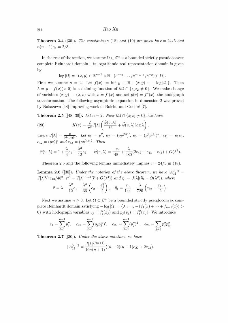
514 Hao Xu
Theorem 2.4 ([30]). The constants in (18) and (19) are given by c = 24/5 and
n(n− 1)cn = 2/3.
In the rest of the section, we assume Ω ⊂ Cn is a bounded strictly pseudoconvex
complete Reinhardt domain. Its logarithmic real representation domain is given
by
− log |Ω| = (x, y) ∈ Rn−1 × R | (e−x1 , . . . , e−xn−1 , e−y) ∈ Ω.
First we assume n = 2. Let f(x) := infy ∈ R | (x, y) ∈ − log |Ω|. Then
λ = y − f(x)(> 0) is a defining function of ∂Ω ∩ z1z2 6= 0. We make change
of variables (x, y) → (λ, v) with v = f ′(x) and set p(v) = f ′′(x), the hodograph
transformation. The following asymptotic expansion in dimension 2 was proved
by Nakazawa [48] improving work of Boichu and Coeure [7].
Theorem 2.5 ([48, 30]). Let n = 2. Near ∂Ω ∩ z1z2 6= 0, we have
(20) K(z) =2
π2J [λ]
(ϕ(v, λ)
λ3+ ψ(v, λ) log λ
),
where J [λ] = p|4z1z2|2 . Let e1 = p′′, e2 = (pp(3))′, e3 = (p2p(4))′′, e41 = e1e3,
e42 = (pe′3)′ and e43 = (pp(4))2. Then
ϕ(v, λ) = 1 +λ
4e1 +
λ2
12e2, ψ(v, λ) =
−e348
+λ
480(2e42 + e43 − e41) +O(λ2).
Theorem 2.5 and the following lemma immediately implies c = 24/5 in (18).
Lemma 2.6 ([30]). Under the notation of the above theorem, we have |A024|2 =
J [λ]4/3e43/482, rF = J [λ]−1/3(r +O(λ4)) and η1 = J [λ](η1 +O(λ2)), where
r = λ−λ2
12e1 −
λ3
36
(e2 −
e212
), η1 =
e3144
−λ
720
(e42 −
e412
).
Next we assume n ≥ 3. Let Ω ⊂ Cn be a bounded strictly pseudoconvex com-
plete Reinhardt domain satisfying − log |Ω| = λ := y− (f1(x)+ · · ·+fn−1(x)) >
0 with hodograph variables vj = f ′j(xj) and pj(vj) = f ′′j (xj). We introduce
e1 =n−1∑
j=1
p′′j , e21 =n−1∑
j=1
(pjp′′′j )′, e22 =
n−1∑
j=1
(p′′j )2, e23 =
∑
j 6=k
p′′jp′′k.
Theorem 2.7 ([30]). Under the above notation, we have
‖A022‖
2 =J [λ]2/(n+1)
16n(n + 1)
((n− 2)(n − 1)e22 + 2e23
),
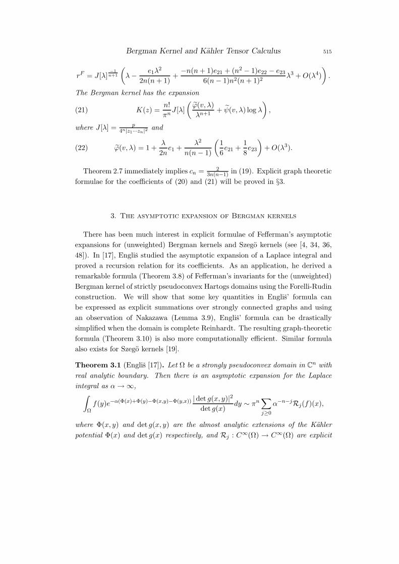
Bergman Kernel and Kahler Tensor Calculus 515
rF = J [λ]−1
n+1
(λ−
e1λ2
2n(n+ 1)+
−n(n+ 1)e21 + (n2 − 1)e22 − e236(n− 1)n2(n+ 1)2
λ3 +O(λ4)
).
The Bergman kernel has the expansion
(21) K(z) =n!
πnJ [λ]
(ϕ(v, λ)
λn+1+ ψ(v, λ) log λ
),
where J [λ] = p4n|z1···zn|2 and
(22) ϕ(v, λ) = 1 +λ
2ne1 +
λ2
n(n− 1)
(1
6e21 +
1
8e23
)+O(λ3).
Theorem 2.7 immediately implies cn = 23n(n−1) in (19). Explicit graph theoretic
formulae for the coefficients of (20) and (21) will be proved in §3.
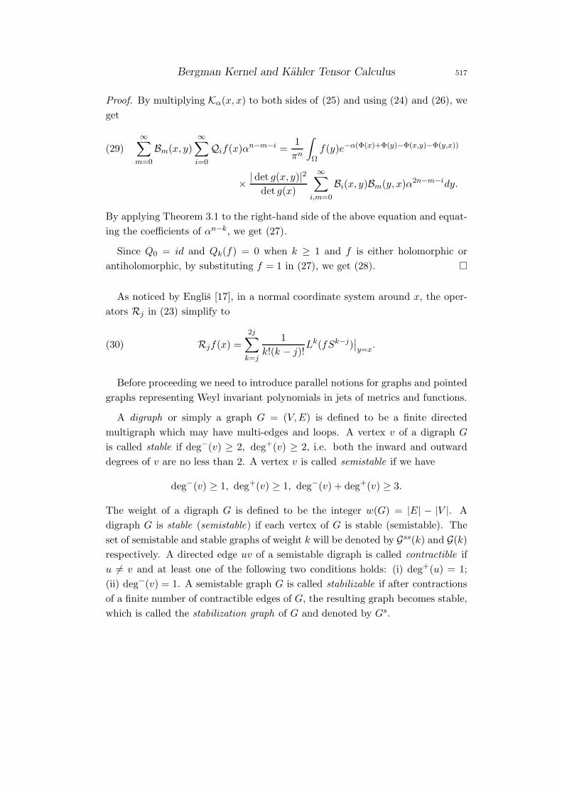
3. The asymptotic expansion of Bergman kernels
There has been much interest in explicit formulae of Fefferman’s asymptotic
expansions for (unweighted) Bergman kernels and Szego kernels (see [4, 34, 36,
48]). In [17], Englis studied the asymptotic expansion of a Laplace integral and
proved a recursion relation for its coefficients. As an application, he derived a
remarkable formula (Theorem 3.8) of Fefferman’s invariants for the (unweighted)
Bergman kernel of strictly pseudoconvex Hartogs domains using the Forelli-Rudin
construction. We will show that some key quantities in Englis’ formula can
be expressed as explicit summations over strongly connected graphs and using
an observation of Nakazawa (Lemma 3.9), Englis’ formula can be drastically
simplified when the domain is complete Reinhardt. The resulting graph-theoretic
formula (Theorem 3.10) is also more computationally efficient. Similar formula
also exists for Szego kernels [19].
Theorem 3.1 (Englis [17]). Let Ω be a strongly pseudoconvex domain in Cn with
real analytic boundary. Then there is an asymptotic expansion for the Laplace
integral as α→ ∞,∫
Ωf(y)e−α(Φ(x)+Φ(y)−Φ(x,y)−Φ(y,x)) |det g(x, y)|2
det g(x)dy ∼ πn
∑
j≥0
α−n−jRj(f)(x),
where Φ(x, y) and det g(x, y) are the almost analytic extensions of the Kahler
potential Φ(x) and det g(x) respectively, and Rj : C∞(Ω) → C∞(Ω) are explicit
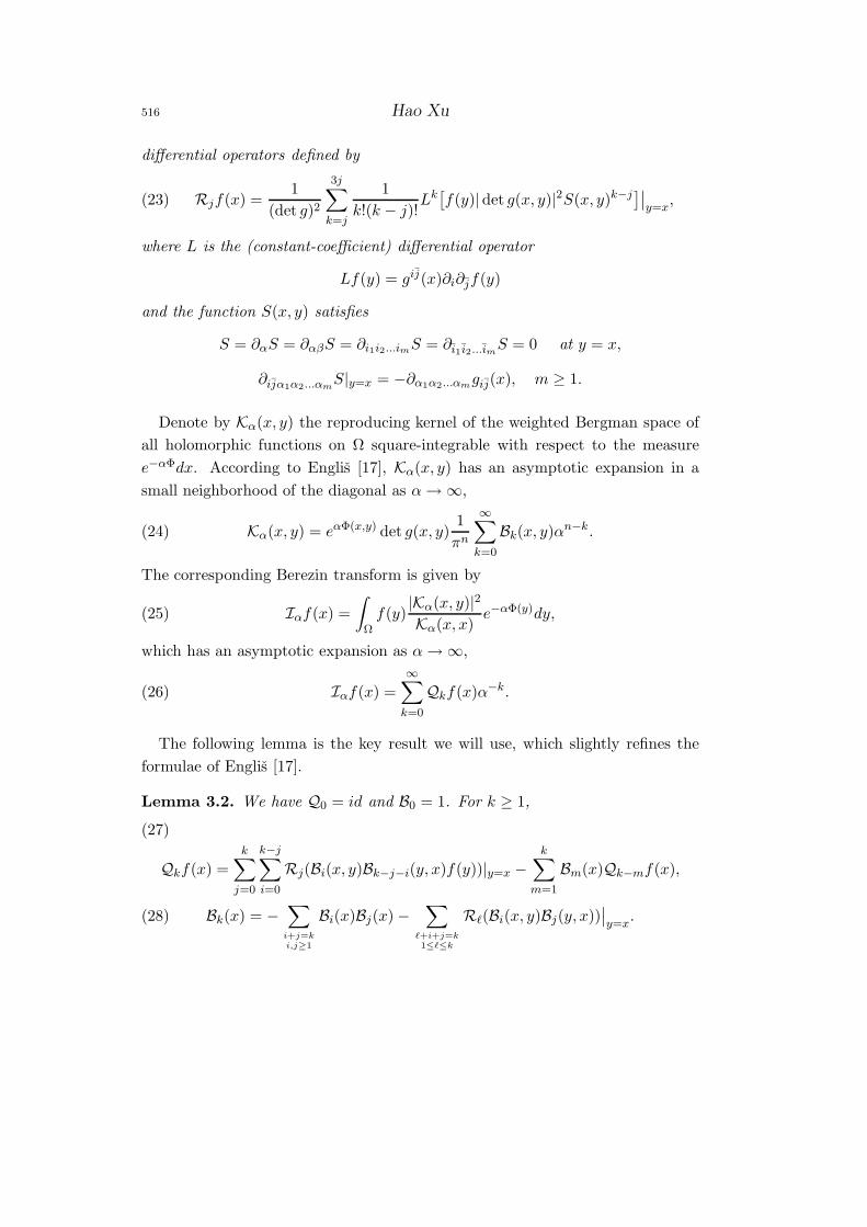
516 Hao Xu
differential operators defined by
(23) Rjf(x) =1
(det g)2
3j∑
k=j
1
k!(k − j)!Lk[f(y)|det g(x, y)|2S(x, y)k−j
]∣∣y=x
,
where L is the (constant-coefficient) differential operator
Lf(y) = gij(x)∂i∂jf(y)
and the function S(x, y) satisfies
S = ∂αS = ∂αβS = ∂i1i2...imS = ∂i1 i2...imS = 0 at y = x,
∂ijα1α2...αmS|y=x = −∂α1α2...αmgij(x), m ≥ 1.
Denote by Kα(x, y) the reproducing kernel of the weighted Bergman space of
all holomorphic functions on Ω square-integrable with respect to the measure
e−αΦdx. According to Englis [17], Kα(x, y) has an asymptotic expansion in a
small neighborhood of the diagonal as α→ ∞,
(24) Kα(x, y) = eαΦ(x,y) det g(x, y)1
πn
∞∑
k=0
Bk(x, y)αn−k.
The corresponding Berezin transform is given by
(25) Iαf(x) =
∫
Ωf(y)
|Kα(x, y)|2
Kα(x, x)e−αΦ(y)dy,
which has an asymptotic expansion as α→ ∞,
(26) Iαf(x) =
∞∑
k=0
Qkf(x)α−k.
The following lemma is the key result we will use, which slightly refines the
formulae of Englis [17].
Lemma 3.2. We have Q0 = id and B0 = 1. For k ≥ 1,
Qkf(x) =
k∑
j=0
k−j∑
i=0
Rj(Bi(x, y)Bk−j−i(y, x)f(y))|y=x −
k∑
m=1
Bm(x)Qk−mf(x),
(27)
Bk(x) = −∑
i+j=ki,j≥1
Bi(x)Bj(x) −∑
ℓ+i+j=k1≤ℓ≤k
Rℓ(Bi(x, y)Bj(y, x))∣∣y=x
.(28)
Bergman Kernel and Kahler Tensor Calculus 517
Proof. By multiplying Kα(x, x) to both sides of (25) and using (24) and (26), we
get
(29)∞∑
m=0
Bm(x, y)∞∑
i=0
Qif(x)αn−m−i =1
πn
∫
Ωf(y)e−α(Φ(x)+Φ(y)−Φ(x,y)−Φ(y,x))
×|det g(x, y)|2
det g(x)
∞∑
i,m=0
Bi(x, y)Bm(y, x)α2n−m−idy.
By applying Theorem 3.1 to the right-hand side of the above equation and equat-
ing the coefficients of αn−k, we get (27).
Since Q0 = id and Qk(f) = 0 when k ≥ 1 and f is either holomorphic or
antiholomorphic, by substituting f = 1 in (27), we get (28).
As noticed by Englis [17], in a normal coordinate system around x, the oper-
ators Rj in (23) simplify to
(30) Rjf(x) =
2j∑
k=j
1
k!(k − j)!Lk(fSk−j)
∣∣y=x
.
Before proceeding we need to introduce parallel notions for graphs and pointed
graphs representing Weyl invariant polynomials in jets of metrics and functions.
A digraph or simply a graph G = (V,E) is defined to be a finite directed
multigraph which may have multi-edges and loops. A vertex v of a digraph G
is called stable if deg−(v) ≥ 2, deg+(v) ≥ 2, i.e. both the inward and outward
degrees of v are no less than 2. A vertex v is called semistable if we have
deg−(v) ≥ 1, deg+(v) ≥ 1, deg−(v) + deg+(v) ≥ 3.
The weight of a digraph G is defined to be the integer w(G) = |E| − |V |. A
digraph G is stable (semistable) if each vertex of G is stable (semistable). The
set of semistable and stable graphs of weight k will be denoted by Gss(k) and G(k)
respectively. A directed edge uv of a semistable digraph is called contractible if
u 6= v and at least one of the following two conditions holds: (i) deg+(u) = 1;
(ii) deg−(v) = 1. A semistable graph G is called stabilizable if after contractions
of a finite number of contractible edges of G, the resulting graph becomes stable,
which is called the stabilization graph of G and denoted by Gs.
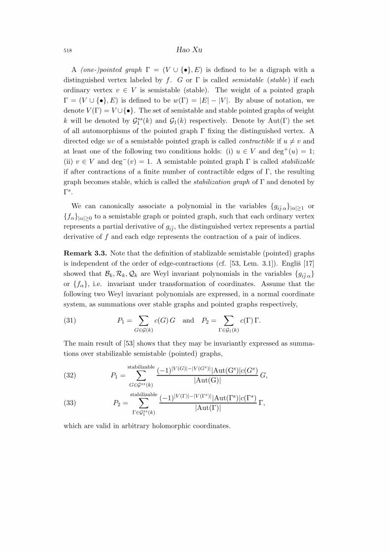
518 Hao Xu
A (one-)pointed graph Γ = (V ∪ •, E) is defined to be a digraph with a
distinguished vertex labeled by f . G or Γ is called semistable (stable) if each
ordinary vertex v ∈ V is semistable (stable). The weight of a pointed graph
Γ = (V ∪ •, E) is defined to be w(Γ) = |E| − |V |. By abuse of notation, we
denote V (Γ) = V ∪•. The set of semistable and stable pointed graphs of weight
k will be denoted by Gss1 (k) and G1(k) respectively. Denote by Aut(Γ) the set
of all automorphisms of the pointed graph Γ fixing the distinguished vertex. A
directed edge uv of a semistable pointed graph is called contractible if u 6= v and
at least one of the following two conditions holds: (i) u ∈ V and deg+(u) = 1;
(ii) v ∈ V and deg−(v) = 1. A semistable pointed graph Γ is called stabilizable
if after contractions of a finite number of contractible edges of Γ, the resulting
graph becomes stable, which is called the stabilization graph of Γ and denoted by
Γs.
We can canonically associate a polynomial in the variables gij α|α|≥1 or
fα|α|≥0 to a semistable graph or pointed graph, such that each ordinary vertex
represents a partial derivative of gij , the distinguished vertex represents a partial
derivative of f and each edge represents the contraction of a pair of indices.
Remark 3.3. Note that the definition of stablizable semistable (pointed) graphs
is independent of the order of edge-contractions (cf. [53, Lem. 3.1]). Englis [17]
showed that Bk,Rk,Qk are Weyl invariant polynomials in the variables gij α
or fα, i.e. invariant under transformation of coordinates. Assume that the
following two Weyl invariant polynomials are expressed, in a normal coordinate
system, as summations over stable graphs and pointed graphs respectively,
(31) P1 =∑
G∈G(k)
c(G)G and P2 =∑
Γ∈G1(k)
c(Γ) Γ.
The main result of [53] shows that they may be invariantly expressed as summa-
tions over stabilizable semistable (pointed) graphs,
P1 =stabilizable∑
G∈Gss(k)
(−1)|V (G)|−|V (Gs)||Aut(Gs)|c(Gs)
|Aut(G)|G,(32)
P2 =stabilizable∑
Γ∈Gss1 (k)
(−1)|V (Γ)|−|V (Γs)||Aut(Γs)|c(Γs)
|Aut(Γ)|Γ,(33)
which are valid in arbitrary holomorphic coordinates.
Bergman Kernel and Kahler Tensor Calculus 519
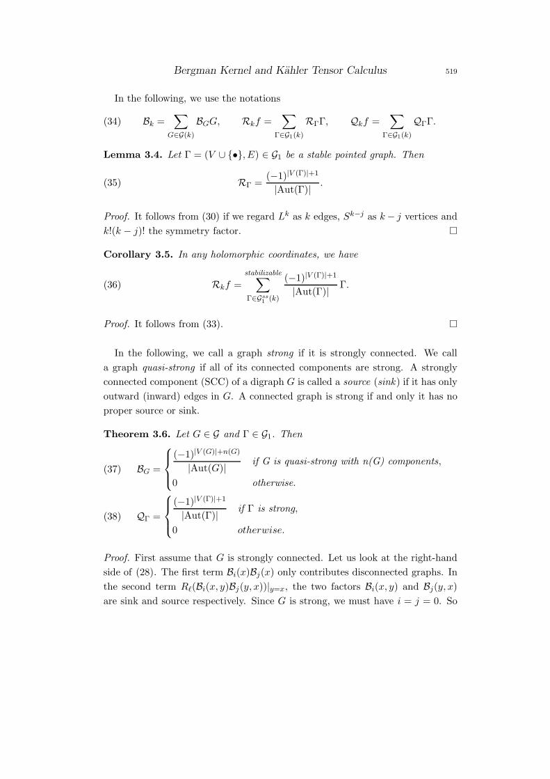
In the following, we use the notations
(34) Bk =∑
G∈G(k)
BGG, Rkf =∑
Γ∈G1(k)
RΓΓ, Qkf =∑
Γ∈G1(k)
QΓΓ.
Lemma 3.4. Let Γ = (V ∪ •, E) ∈ G1 be a stable pointed graph. Then
(35) RΓ =(−1)|V (Γ)|+1
|Aut(Γ)|.
Proof. It follows from (30) if we regard Lk as k edges, Sk−j as k− j vertices and
k!(k − j)! the symmetry factor.
Corollary 3.5. In any holomorphic coordinates, we have
(36) Rkf =
stabilizable∑
Γ∈Gss1 (k)
(−1)|V (Γ)|+1
|Aut(Γ)|Γ.
Proof. It follows from (33).
In the following, we call a graph strong if it is strongly connected. We call
a graph quasi-strong if all of its connected components are strong. A strongly
connected component (SCC) of a digraph G is called a source (sink) if it has only
outward (inward) edges in G. A connected graph is strong if and only it has no
proper source or sink.
Theorem 3.6. Let G ∈ G and Γ ∈ G1. Then
BG =
(−1)|V (G)|+n(G)
|Aut(G)|if G is quasi-strong with n(G) components,
0 otherwise.
(37)
QΓ =
(−1)|V (Γ)|+1
|Aut(Γ)|if Γ is strong,
0 otherwise.
(38)
Proof. First assume that G is strongly connected. Let us look at the right-hand
side of (28). The first term Bi(x)Bj(x) only contributes disconnected graphs. In
the second term Rℓ(Bi(x, y)Bj(y, x))|y=x, the two factors Bi(x, y) and Bj(y, x)
are sink and source respectively. Since G is strong, we must have i = j = 0. So
520 Hao Xu
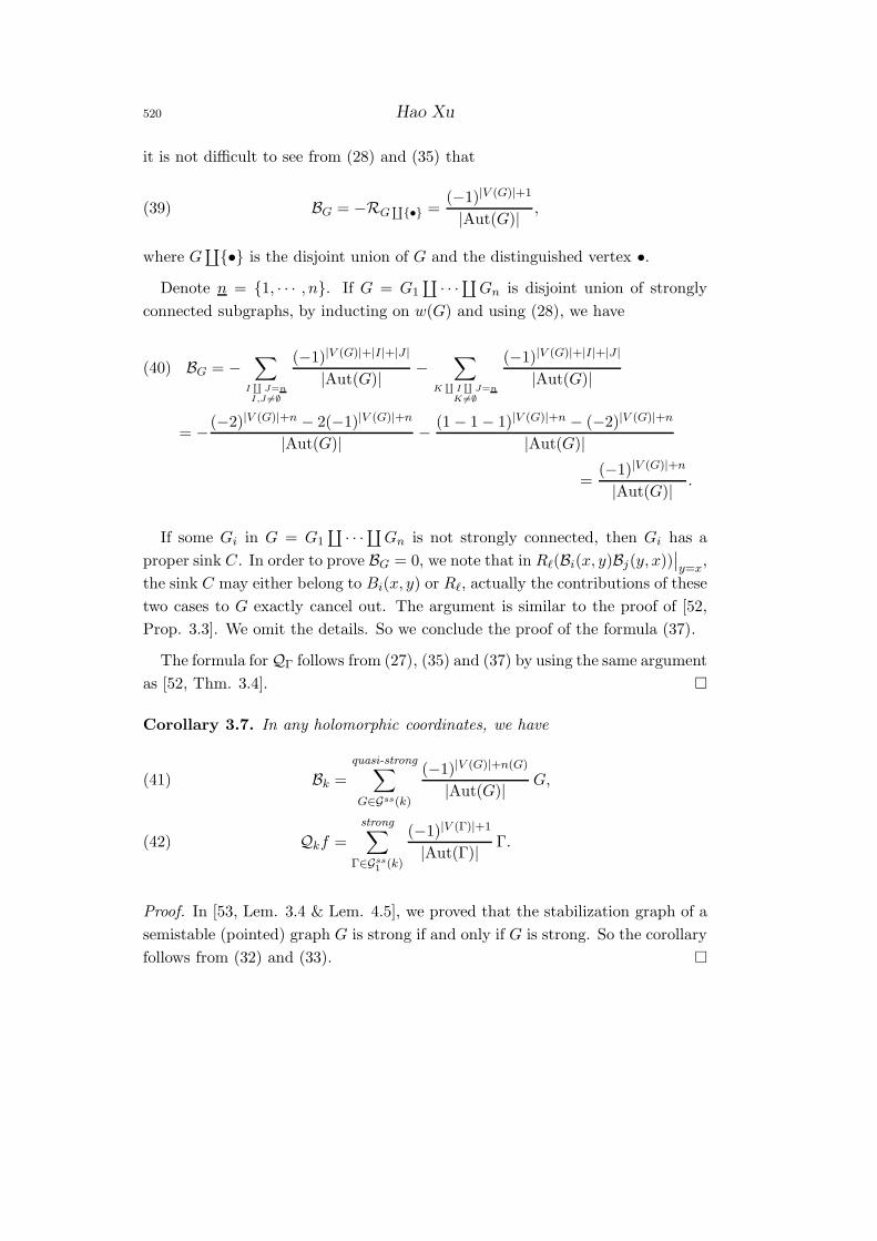
it is not difficult to see from (28) and (35) that
(39) BG = −RG∐
• =(−1)|V (G)|+1
|Aut(G)|,
where G∐• is the disjoint union of G and the distinguished vertex •.
Denote n = 1, · · · , n. If G = G1∐
· · ·∐Gn is disjoint union of strongly
connected subgraphs, by inducting on w(G) and using (28), we have
(40) BG = −∑
I∐
J=n
I,J 6=∅
(−1)|V (G)|+|I|+|J |
|Aut(G)|−
∑
K∐
I∐
J=n
K 6=∅
(−1)|V (G)|+|I|+|J |
|Aut(G)|
= −(−2)|V (G)|+n − 2(−1)|V (G)|+n
|Aut(G)|−
(1 − 1 − 1)|V (G)|+n − (−2)|V (G)|+n
|Aut(G)|
=(−1)|V (G)|+n
|Aut(G)|.
If some Gi in G = G1∐
· · ·∐Gn is not strongly connected, then Gi has a
proper sink C. In order to prove BG = 0, we note that in Rℓ(Bi(x, y)Bj(y, x))∣∣y=x
,
the sink C may either belong to Bi(x, y) or Rℓ, actually the contributions of these
two cases to G exactly cancel out. The argument is similar to the proof of [52,
Prop. 3.3]. We omit the details. So we conclude the proof of the formula (37).
The formula for QΓ follows from (27), (35) and (37) by using the same argument
as [52, Thm. 3.4].
Corollary 3.7. In any holomorphic coordinates, we have
Bk =
quasi-strong∑
G∈Gss(k)
(−1)|V (G)|+n(G)
|Aut(G)|G,(41)
Qkf =
strong∑
Γ∈Gss1 (k)
(−1)|V (Γ)|+1
|Aut(Γ)|Γ.(42)
Proof. In [53, Lem. 3.4 & Lem. 4.5], we proved that the stabilization graph of a
semistable (pointed) graph G is strong if and only if G is strong. So the corollary
follows from (32) and (33).
Bergman Kernel and Kahler Tensor Calculus 521
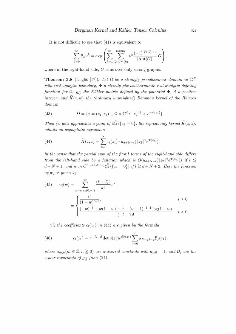
It is not difficult to see that (41) is equivalent to
∞∑
k=0
Bkνk = exp
∞∑
k=1
strong∑
G∈Gss(k)
νk (−1)|V (G)|+1
|Aut(G)|G
,
where in the right-hand side, G runs over only strong graphs.
Theorem 3.8 (Englis [17]). Let Ω be a strongly pseudoconvex domain in CN
with real-analytic boundary, Φ a strictly plurisubharmonic real-analytic defining
function for Ω, gij the Kahler metric defined by the potential Φ, d a positive
integer, and K(z,w) the (ordinary unweighted) Bergman kernel of the Hartogs
domain
(43) Ω = z = (z1, z2) ∈ Ω × Cd : ‖z2‖
2 < e−Φ(z1).
Then (i) as z approaches a point of ∂Ω\z2 = 0, the reproducing kernel K(z, z).
admits an asymptotic expansion
(44) K(z, z) =
∞∑
l=0
cl(z1) · ud+N−l(‖z2‖2eΦ(z1)),
in the sense that the partial sum of the first l terms of the right-hand side differs
from the left-hand side by a function which is O(ud+N−l(‖z2‖2eΦ(z1))) if l ≦
d+N + 1, and is in C l−(d+N+2)(Ω\z2 = 0) if l ≧ d+N + 2. Here the function
ul(w) is given by
ul(w) =
∞∑
k=max(0,−l)
(k + l)!
k!wk(45)
=
l!
(1 − w)l+1, l ≥ 0,
(−w)−l + w(1 − w)−l−1 − (w − 1)−l−1 log(1 − w)
(−l − 1)!, l < 0.
(ii) the coefficients cl(z1) in (44) are given by the formula
(46) cl(z1) = π−N−d det g(z1)edΦ(z1)
l∑
j=0
aN−j,l−jBj(z1),
where am,n(m ∈ Z, n ≧ 0) are universal constants with am0 = 1, and Bj are the
scalar invariants of gij from (24).
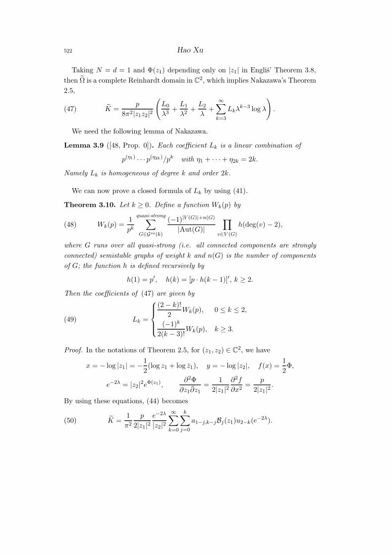
522 Hao Xu
Taking N = d = 1 and Φ(z1) depending only on |z1| in Englis’ Theorem 3.8,
then Ω is a complete Reinhardt domain in C2, which implies Nakazawa’s Theorem
2.5,
(47) K =p
8π2|z1z2|2
(L0
λ3+L1
λ2+L2
λ+
∞∑
k=3
Lkλk−3 log λ
).
We need the following lemma of Nakazawa.
Lemma 3.9 ([48, Prop. 0]). Each coefficient Lk is a linear combination of
p(η1) · · · p(η2k)/pk with η1 + · · · + η2k = 2k.
Namely Lk is homogeneous of degree k and order 2k.
We can now prove a closed formula of Lk by using (41).
Theorem 3.10. Let k ≥ 0. Define a function Wk(p) by
(48) Wk(p) =1
pk
quasi-strong∑
G∈Gss(k)
(−1)|V (G)|+n(G)
|Aut(G)|
∏
v∈V (G)
h(deg(v) − 2),
where G runs over all quasi-strong (i.e. all connected components are strongly
connected) semistable graphs of weight k and n(G) is the number of components
of G; the function h is defined recursively by
h(1) = p′, h(k) = [p · h(k − 1)]′, k ≥ 2.
Then the coefficients of (47) are given by
(49) Lk =
(2 − k)!
2Wk(p), 0 ≤ k ≤ 2,
(−1)k
2(k − 3)!Wk(p), k ≥ 3.
Proof. In the notations of Theorem 2.5, for (z1, z2) ∈ C2, we have
x = − log |z1| = −1
2(log z1 + log z1), y = − log |z2|, f(x) =
1
2Φ,
e−2λ = |z2|2eΦ(z1),
∂2Φ
∂z1∂z1=
1
2|z1|2∂2f
∂x2=
p
2|z1|2.
By using these equations, (44) becomes
(50) K =1
π2
p
2|z1|2e−2λ
|z2|2
∞∑
k=0
k∑
j=0
a1−j,k−jBj(z1)u2−k(e−2λ).
Bergman Kernel and Kahler Tensor Calculus 523
By (45), the singular part of u2−k(e−2λ) is given by
(51) u2−k(e−2λ) =
(2 − k)! +O(λ)
23−kλ3−k, 0 ≤ k ≤ 2,
[(−1)k2k−3λk−3 +O(λk−2)] log(λ)
(k − 3)!, k ≥ 3.
Note that the derivatives of p satisfy
(52)∂p
∂z1= −
pp′
2z1,
∂p
∂z1= −
pp′
2z1.
By (41), we express Bj(z1) as a summation of rational differential functions of p,
(53) Bj(z1) =
quasi-strong∑
G∈Gss(j)
(−1)|V (G)|+n(G)
|Aut(G)|
×∏
v∈V (G)
∂deg(v)−2
∂zdeg+(v)−11 ∂z
deg−(v)−11
[p
2|z1|2
] ∣∣∣∣|z1|2=p/2
.
Note that Bj is of degree no more than j. The top degree is achieved only when
all derivatives are taken on the numerator p. It is not difficult to see from (53)
that
Bj(z1) =
quasi-strong∑
G∈Gss(j)
(−1)|V (G)|+n(G)
|Aut(G)|
1
2jpj
∏
v∈V (G)
1
p·
∂deg(v)−2p
∂zdeg+(v)−11 ∂z
deg−(v)−11
+ Low
=
quasi-strong∑
G∈Gss(j)
(−1)|V (G)|+n(G)
|Aut(G)|
1
2jpj
∏
v∈V (G)
h(deg(v) − 2) + Low
=Wj(p)
2j+ Low,
where Low denotes the terms of rational differential functions of p with degree
strictly less than j, which may be discarded according to Lemma 3.9. It also
implies that in the summation (50), we can discard all terms except when j = k,
i.e. the term a1−k,0Bk(z1) = Bk(z1). In view of (51), Equation (49) follows
immediately.
Remark 3.11. The formula (48) may be reformulated as
(54) Wk(p) =1
pk
quasi-strong∑
H
(−1)|V (H)|+n(H)
|V (H)|! (|V (H)| + k)!
∏
v∈V (H)
h(deg(v) − 2),
524 Hao Xu
where H runs over isomorphism classes of labeled semistable quasi-strong graphs
of weight k, i.e. the vertices and edges of H are labeled by 1, . . . , |V (H)|
and 1, . . . , |E(H)| respectively. Denote by N(d1, . . . , dj) the number of labeled
strong graphs with given degree sequence (d1, . . . , dj). The computation with
(54) will be greatly eased if one can find a recursive formula for N(d1, . . . , dj),
e.g. using the method of [38].
Example 3.12. Obviously L0 = W0(p) = 1. Note that
h(1) = p′, h(2) = (p′)2 + pp′′,
h(3) = (p′)3 + 4pp′p′′ + p2p(3),
h(4) = (p′)4 + 11p(p′)2p′′ + 7p2p′p(3) + 4p2(p′′)2 + p3p(4).
We now compute L1, L2, L3 by using Theorem 3.10. There are two quasi-strong
graphs in Gss(1),
[765401232] [
2
))
1
ii
]
So W1(p) = 1p(h(2)
2 − h(1)2
2 ) = 12p
′′, which implies L1 = 14p
′′.
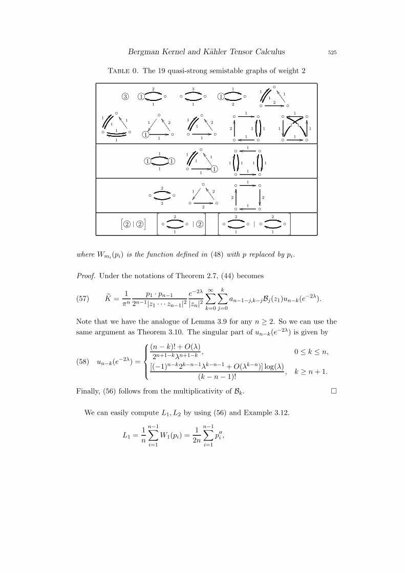
There are 19 quasi-strong graphs in Gss(2) as depicted in Table 0, among which
4 are stable. They are grouped according to their stabilization graphs. It is a
routine calculation that W2(p) = 16 (pp(3))′, which implies L2 = 1
12 (pp(3))′.
There are 300 quasi-strong graphs in Gss(3), among which 14 are stable. With
the help of Maple, we get W3(p) = 124(p2p(4))′′, which implies L3 = − 1
48(p2p(4))′′.
Now we consider the higher dimensional Reinhardt domains. Let n ≥ 2. Under
the notations of Theorem 2.7, denote
(55) K =n! p1 · · · pn−1
4nπn|z1 · · · zn|2
(n∑
k=0
Lk
λn+1−k+
∞∑
k=n+1
Lkλk−(n+1) log λ
).
Theorem 3.13. Let k ≥ 0. Then the coefficients of (55) are given by
(56) Lk =
(n− k)!
n!
∑
k=m1+···+mn−1mi≥0
n−1∏
i=1
Wmi(pi), 0 ≤ k ≤ n,
(−1)n−k
n!(k − 1 − n)!
∑
k=m1+···+mn−1mi≥0
n−1∏
i=1
Wmi(pi), k ≥ n+ 1,
Bergman Kernel and Kahler Tensor Calculus 525
Table 0. The 19 quasi-strong semistable graphs of weight 2
'&%$ !"#3 '&%$ !"#1
2((
1
hh
3((
1
hh '&%$ !"#1
1((
2
hh
1
1<<
2 //
1ZZ66666
1
1<<
1 33 1
kk
1ZZ66666
1
'&%$ !"#11
//
2ZZ55555
1
1<<
1//
2ZZ66666
1 //
1
2
OO
1
JJ
1oo
1
1
1oo
1
55
1 //
1
OO
'&%$ !"#1
1(( '&%$ !"#1
1
hh
1
1<<
1// '&%$ !"#1
1ZZ55555
1
1oo
1
1
JJ
1 //
1
JJ
2((
2
hh
1
2
//
2ZZ66666
1 //
2
2
OO
1oo
['&%$ !"#2 | '&%$ !"#2
]
2((
1
hh | '&%$ !"#2
2((
1
hh | 2
((
1
hh
where Wmi(pi) is the function defined in (48) with p replaced by pi.
Proof. Under the notations of Theorem 2.7, (44) becomes
(57) K =1
πn
p1 · pn−1
2n−1|z1 · · · zn−1|2e−2λ
|zn|2
∞∑
k=0
k∑
j=0
an−1−j,k−jBj(z1)un−k(e−2λ).
Note that we have the analogue of Lemma 3.9 for any n ≥ 2. So we can use the
same argument as Theorem 3.10. The singular part of un−k(e−2λ) is given by
(58) un−k(e−2λ) =
(n − k)! +O(λ)
2n+1−kλn+1−k, 0 ≤ k ≤ n,
[(−1)n−k2k−n−1λk−n−1 +O(λk−n)] log(λ)
(k − n− 1)!, k ≥ n+ 1.
Finally, (56) follows from the multiplicativity of Bk.
We can easily compute L1, L2 by using (56) and Example 3.12.
L1 =1
n
n−1∑
i=1
W1(pi) =1
2n
n−1∑
i=1
p′′i ,
526 Hao Xu
L2 =1
n(n− 1)
n−1∑
i=1
W2(pi) +1
2
∑
i6=j
W1(pi)W1(pj)
=1
n(n− 1)
1
6
n−1∑
i=1
(pip(3)i )′ +
1
8
∑
i6=j
p′′i p′′j
,
which agree with (22).
4. From partial to covariant derivatives
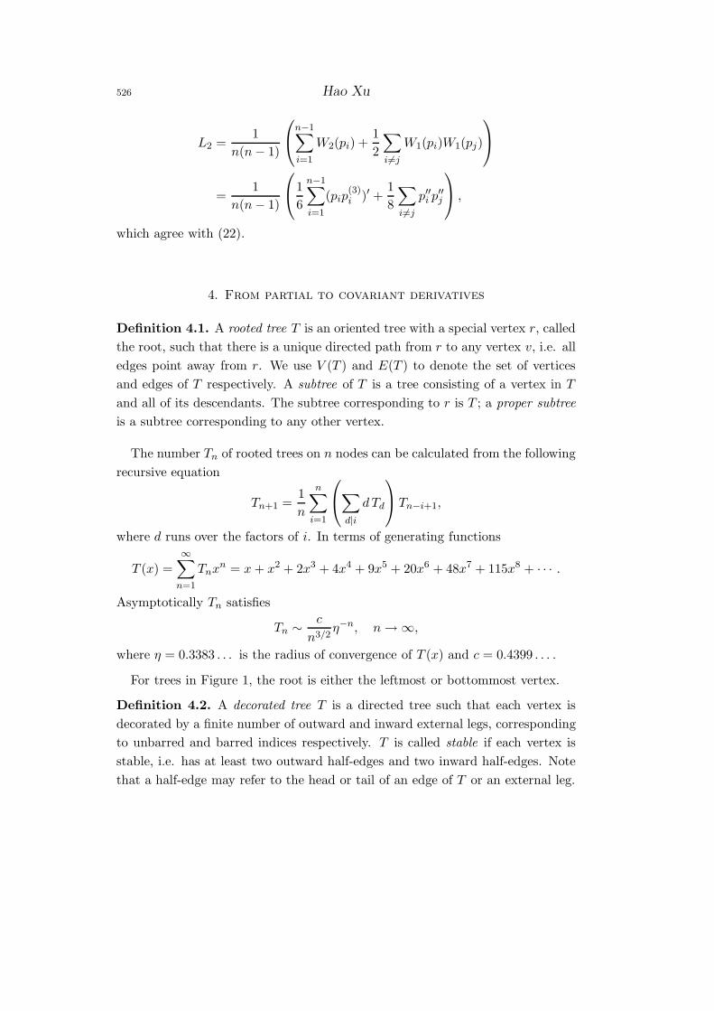
Definition 4.1. A rooted tree T is an oriented tree with a special vertex r, called
the root, such that there is a unique directed path from r to any vertex v, i.e. all
edges point away from r. We use V (T ) and E(T ) to denote the set of vertices
and edges of T respectively. A subtree of T is a tree consisting of a vertex in T
and all of its descendants. The subtree corresponding to r is T ; a proper subtree
is a subtree corresponding to any other vertex.
The number Tn of rooted trees on n nodes can be calculated from the following
recursive equation
Tn+1 =1
n
n∑
i=1
∑
d|idTd
Tn−i+1,
where d runs over the factors of i. In terms of generating functions
T (x) =
∞∑
n=1
Tnxn = x+ x2 + 2x3 + 4x4 + 9x5 + 20x6 + 48x7 + 115x8 + · · · .
Asymptotically Tn satisfies
Tn ∼c
n3/2η−n, n→ ∞,
where η = 0.3383 . . . is the radius of convergence of T (x) and c = 0.4399 . . . .
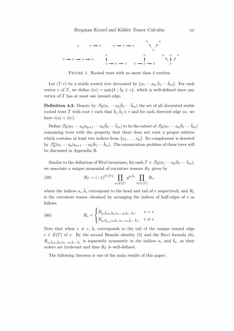
For trees in Figure 1, the root is either the leftmost or bottommost vertex.
Definition 4.2. A decorated tree T is a directed tree such that each vertex is
decorated by a finite number of outward and inward external legs, corresponding
to unbarred and barred indices respectively. T is called stable if each vertex is
stable, i.e. has at least two outward half-edges and two inward half-edges. Note
that a half-edge may refer to the head or tail of an edge of T or an external leg.
Bergman Kernel and Kahler Tensor Calculus 527
// // //
CC[[777
// // //
//
OO
//
//
OO
//
AAOO]]<<<
Figure 1. Rooted trees with no more than 4 vertices
Let (T, r) be a stable rooted tree decorated by a1 · · · ak, b1 · · · bm. For each
vertex v of T , we define i(v) = mink | bk ∈ v, which is well-defined since any
vertex of T has at most one inward edge.
Definition 4.3. Denote by TR(a1 · · · ak|b1 · · · bm) the set of all decorated stable
rooted trees T with root r such that b1, b2 ∈ r and for each directed edge uv, we
have i(u) < i(v).
Define TR(a1 · · · ap|ap+1 · · · ak|b1 · · · bm) to be the subset of TR(a1 · · · ak|b1 · · · bm)
containing trees with the property that there does not exist a proper subtree
which contains at least two indices from a1, . . . , ap. Its complement is denoted
by T cR(a1 · · · ap|ap+1 · · · ak|b1 · · · bm). The enumeration problem of these trees will
be discussed in Appendix B.
Similar to the definition of Weyl invariants, for each T ∈ TR(a1 · · · ak|b1 · · · bm),
we associate a unique monomial of curvature tensors RT given by
(59) RT = (−1)|V (T )| ∏
e∈E(T )
gae be∏
v∈V (T )
Rv,
where the indices ae, be correspond to the head and tail of e respectively and Rv
is the curvature tensor obtained by arranging the indices of half-edges of v as
follows
(60) Rv =
Ra∗b1a∗b2/a∗···a∗b∗···b∗ , v = r,
Ra∗bi(v)a∗be/a∗···a∗ b∗···b∗ , v 6= r.
Note that when v 6= r, be corresponds to the tail of the unique inward edge
e ∈ E(T ) of v. By the second Bianchi identity (5) and the Ricci formula (6),
Ra∗ b1a∗ b2/a∗···a∗ b∗···b∗ is separately symmetric in the indices a∗ and b∗, so their
orders are irrelevant and thus RT is well-defined.
The following theorem is one of the main results of this paper.
528 Hao Xu
Theorem 4.4. Let k ≥ p ≥ 2 and m ≥ 2. Then
D((grsgrb1 b2
ga1 sa2)a3···ak b3···bm
)=
∑
T∈T cR
(a1a2|a3···ak|b1···bm)
RT ,(61)
−D((Ra1 b1a2 b2/a3···ap
)ap+1···ak b3···bm
)=
∑
T∈TR(a1···ap|ap+1···ak |b1···bm)
RT ,(62)
D(ga1 b1a2 b2a3···ak b3···bm) =
∑
T∈TR(a1···ak |b1···bm)
RT .(63)
Proof. First the theorem is obviously true when k = m = 2 or p = k. We will
proceed by induction.
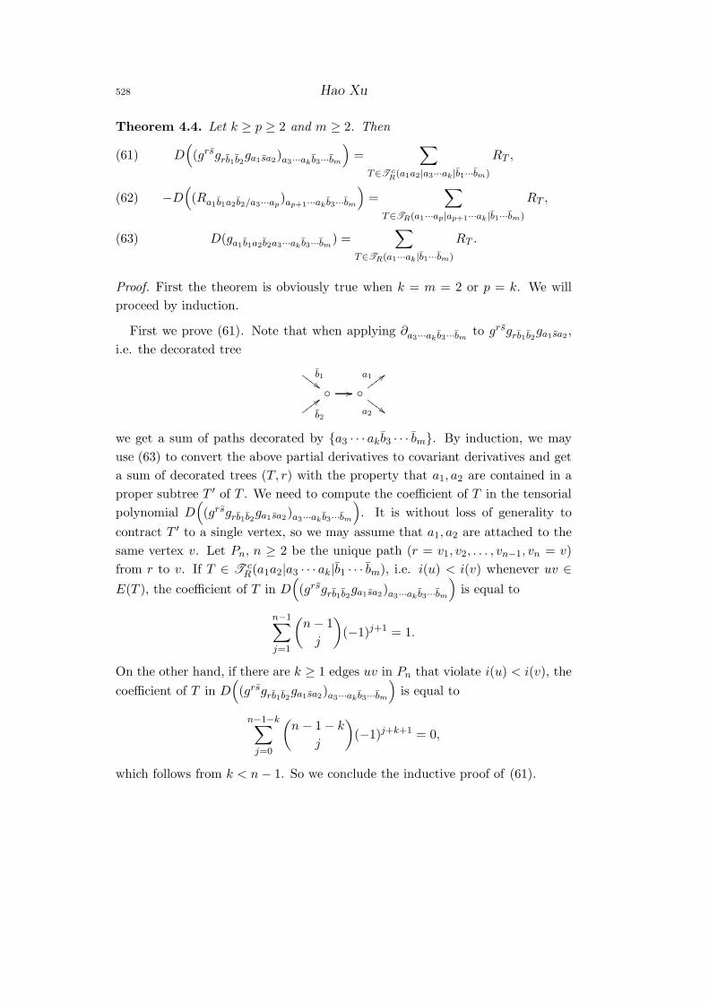
First we prove (61). Note that when applying ∂a3···ak b3···bmto grsgrb1 b2
ga1sa2 ,
i.e. the decorated tree
b1##GG
GG
//
a1 ;;wwww
a2 ##GGGG
b2
;;wwww
we get a sum of paths decorated by a3 · · · ak b3 · · · bm. By induction, we may
use (63) to convert the above partial derivatives to covariant derivatives and get
a sum of decorated trees (T, r) with the property that a1, a2 are contained in a
proper subtree T ′ of T . We need to compute the coefficient of T in the tensorial
polynomial D((grsgrb1b2ga1 sa2)a3···ak b3···bm
). It is without loss of generality to
contract T ′ to a single vertex, so we may assume that a1, a2 are attached to the
same vertex v. Let Pn, n ≥ 2 be the unique path (r = v1, v2, . . . , vn−1, vn = v)
from r to v. If T ∈ T cR(a1a2|a3 · · · ak|b1 · · · bm), i.e. i(u) < i(v) whenever uv ∈
E(T ), the coefficient of T in D((grsgrb1 b2
ga1sa2)a3···ak b3···bm
)is equal to
n−1∑
j=1
(n− 1
j
)(−1)j+1 = 1.
On the other hand, if there are k ≥ 1 edges uv in Pn that violate i(u) < i(v), the
coefficient of T in D((grsgrb1 b2
ga1sa2)a3···ak b3···bm
)is equal to
n−1−k∑
j=0
(n− 1 − k
j
)(−1)j+k+1 = 0,
which follows from k < n− 1. So we conclude the inductive proof of (61).
Bergman Kernel and Kahler Tensor Calculus 529
Next we prove (62). Note that (62) holds when p = k by (8). From (2), we
have
(64) (Ra1 b1a2 b2/a3···ap)ap+1···ak b3···bm
= (Ra1 b1a2 b2/a3···apap+1)ap+2···ak b3···bm
+ (grsgap+1sa1Rrb1a2 b2/a3···ap+ grsgap+1sa2Ra1 b1rb2/a3···ap
)ap+2···ak b3···bm
+
p∑
j=3
(grsgap+1sajRa1 b1a2 b2/a3···aj−1raj+1···ap
)ap+2···ak b3···bm.
Then by induction, in the right-hand side of (64), the first term produces trees
with the property that no two of a1, . . . , ap, ap+1 are contained in a proper
subtree, the second term produces trees with the property that either a1, ap+1
or a2, ap+1 are contained in a proper subtree, the last term produces trees with
the property that aj, ap+1 (3 ≤ j ≤ p) are contained in a proper subtree. The
coefficient of each tree can be determined by exactly the same argument as in the
above proof of (61). So we conclude the inductive proof of (62).
Finally we prove (63). By (1), we have
ga1 b1a2 b2a3···ak b3···bm= −(Ra1 b1a2 b2)a3···ak b3···bm
+ (grsgrb1 b2ga1 sa2)a3···ak b3···bm.
So the expression of D(ga1 b1a2 b2a3···ak b3···bm) in (63) follows directly from (61)
and the p = 2 case of (62). Therefore we conclude the inductive proof of the
theorem.
Remark 4.5. See [54] for related results more general than Theorem 4.4.
We sort indices in alphabetical order, i, j, k, l, p, q, . . . . Note that only the order
of barred indices is essential.
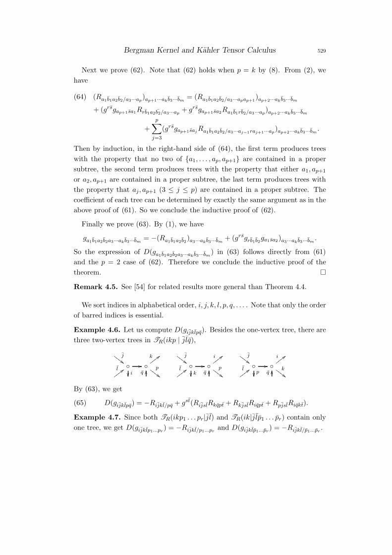
Example 4.6. Let us compute D(gijklpq). Besides the one-vertex tree, there are
three two-vertex trees in TR(ikp | jlq),
j##GG
GG
//i
k ;;wwwwp
##GGGGl ;;wwww
qOO
j##GG
GG
//k
i ;;wwwwp
##GGGGl ;;wwww
qOO
j##GG
GG
//p
i ;;wwwwk
##GGGGl ;;wwww
qOO
By (63), we get
(65) D(gijklpq) = −Rijkl/pq + gst(RijslRkqpt +RkjslRiqpt +RpjslRiqkt).
Example 4.7. Since both TR(ikp1 . . . pr|j l) and TR(ik|j lp1 . . . pr) contain only
one tree, we get D(gijklp1...pr) = −Rijkl/p1...pr
and D(gijklp1...pr) = −Rijkl/p1...pr
.

530 Hao Xu
The next theorem shows the difference when we interchange two non-adjacent
barred indices in a curvature tensor.
Theorem 4.8. Let m ≥ 3. Then
(66) Ra1 b1a2 b2/a3···ak b3···bm−Ra1 b1a2 b3/a3···ak b2 b4···bm
=∑
T
η(T )RT ,
where T = ue→ v runs over stable two-vertex paths decorated by indices
a1 · · · ak, b1 · · · bm and
(67) η(T ) =
1, if b1, b2 ∈ u and b3 ∈ v,
−1, if b1, b3 ∈ u and b2 ∈ v,
0, otherwise.
The curvature tensor RT corresponding to T is given by (cf. (80))
RT =
Ra∗b1a∗b2/a∗···a∗b∗···b∗Ra∗b3a∗be/a∗···a∗b∗···b∗ , if b1, b2 ∈ u and b3 ∈ v,
Ra∗b1a∗b3/a∗···a∗b∗···b∗Ra∗b2a∗be/a∗···a∗b∗···b∗ , if b1, b3 ∈ u and b2 ∈ v.
Proof. The left-hand side of (66) is equal to
(68)
k∑
j=3
(Ra1 b1a2 b2/a3···aj b3aj+1···ak b4···bm
−Ra1 b1a2 b2/a3···aj−1 b3aj ···ak b4···bm
)
−k∑
j=3
(Ra1 b1a2 b3/a3···aj b2aj+1···ak b4···bm
−Ra1 b1a2 b3/a3···aj−1 b2aj ···ak b4···bm
)
By the Ricci formula (7), it is not difficult to see that any two-vertex path T =
ue→ v appearing in (68) must satisfy one of the following conditions:
(i) b1, b2 ∈ u, b3 ∈ v; (ii) b1, b3 ∈ u, b2 ∈ v; (iii) b2, b3 ∈ u, b1 ∈ v.
Again by the Ricci formula (7), the contributions of the two summations in
(68) to (iii) cancel out.
A two-vertex path T in (i) is contained in the first (resp. second) summation
in (68) if and only if at least one of a1, a2 belongs to u (resp. both a1, a2 belong
to v).
A two-vertex path T in (ii) is contained in the first (resp. second) summation
in (68) if and only if both a1, a2 belong to v (resp. at least one of a1, a2 belongs
to u).
Bergman Kernel and Kahler Tensor Calculus 531
Finally, (68) follows by noting that T in (i) and (ii) has multiplicity 1 and −1
respectively.
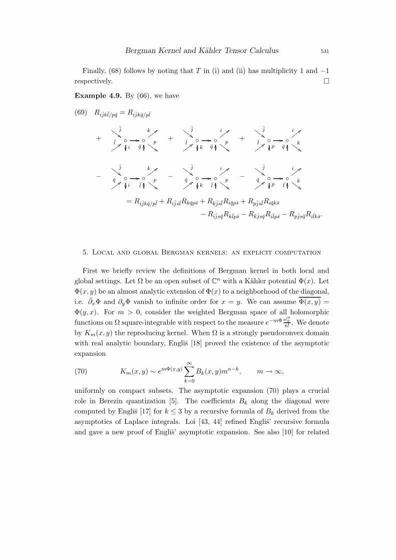
Example 4.9. By (66), we have
(69) Rijkl/pq = Rijkq/pl
+
j##GG
GG
//i
k ;;wwwwp
##GGGGl ;;wwww
qOO
+
j##GG
GG
//k
i ;;wwwwp
##GGGGl ;;wwww
qOO
+
j##GG
GG
//p
i ;;wwwwk
##GGGGl ;;wwww
qOO
−
j##GG
GG
//i
k ;;wwwwp
##GGGGq ;;wwww l
OO−
j##GG
GG
//k
i ;;wwwwp
##GGGGq ;;wwww l
OO−
j##GG
GG
//p
i ;;wwwwk
##GGGGq ;;wwww l
OO
= Rijkq/pl +RijslRkqps +RkjslRiqps +RpjslRiqks
−RijsqRklps −RkjsqRilps −RpjsqRilks.
5. Local and global Bergman kernels: an explicit computation
First we briefly review the definitions of Bergman kernel in both local and
global settings. Let Ω be an open subset of Cn with a Kahler potential Φ(x). Let
Φ(x, y) be an almost analytic extension of Φ(x) to a neighborhood of the diagonal,
i.e. ∂xΦ and ∂yΦ vanish to infinite order for x = y. We can assume Φ(x, y) =
Φ(y, x). For m > 0, consider the weighted Bergman space of all holomorphic
functions on Ω square-integrable with respect to the measure e−mΦ ωng
n! . We denote
by Km(x, y) the reproducing kernel. When Ω is a strongly pseudoconvex domain
with real analytic boundary, Englis [18] proved the existence of the asymptotic
expansion
(70) Km(x, y) ∼ emΦ(x,y)∞∑
k=0
Bk(x, y)mn−k, m→ ∞,
uniformly on compact subsets. The asymptotic expansion (70) plays a crucial
role in Berezin quantization [5]. The coefficients Bk along the diagonal were
computed by Englis [17] for k ≤ 3 by a recursive formula of Bk derived from the
asymptotics of Laplace integrals. Loi [43, 44] refined Englis’ recursive formula
and gave a new proof of Englis’ asymptotic expansion. See also [10] for related
532 Hao Xu
works. As shown in [43] (also cf. [51, §3]), Bk is equal to ak of (71) in the global
case.
For a compact Kahler manifold M of dimension n, instead of holomorphic
functions, we consider holomorphic sections of holomorphic line bundles. Let
(L, h) → M be a positive Hermitian holomorphic line bundle and g be the po-
larized Kahler metric on M corresponding to the Kahler form ωg = Ric(h). For
each m ∈ N, h induces a Hermitian metric hm on Lm. Let S1, · · · , Sd be an
orthonormal basis of H0(M,Lm) with respect to the inner product
(Si, Sj)hm=
∫
Mhm(Si(x), Sj(x))
1
n!ωn
g .
Zelditch [57] and Catlin [9] independently proved that there is a complete asymp-
totic expansion:
(71)d∑
i=0
‖Si(x)‖2hm
= a0(x)mn + a1(x)m
n−1 + a2(x)mn−2 + · · ·
Various extensions to off-diagonal asymptotic expansion and generalizations to
orbifolds and symplectic manifolds can be found in e.g. [6, 13, 14, 35, 46, 49].
See also recent works [2, 16, 24, 33, 42].
The ak for k ≤ 3 were computed by Lu [45] using peak section method. In
particular,
a0 = 1, a1 =ρ
2, a2 =
1
3∆ρ+
1
24|R|2 −
1
6|Ric|2 +
1
8ρ2.
The computation of a3, independently done by Lu [45] and Englis [17], is a
marvelous feat; this requires technical and hard calculations occupying more than
ten pages in both papers.
In the rest of the section, we use results proved in §4 to give a relatively easy
derivation of the tensor expression for a3. The following explicit closed formula
of ak was proved in [51, 52],
(72) Bk(x) = ak(x) =∑
G
z(G) ·G =∑
G
(−1)n det(A− I)
|Aut(G)|G,
where G = G1∪· · ·∪Gn runs over stable (i.e. both the indegree and outdegree of
each vertex are no less than 2) multi-digraphs of weight k (i.e. |E(G)|− |V (G)| =
k) such that each component Gi is strongly connected and A is the adjacency
matrix of G. Although (72) gives a closed formula of ak as a summation of local
Bergman Kernel and Kahler Tensor Calculus 533
partial derivatives, it is still a quite hard task to convert it into tensor expressions
when k ≥ 3.
We will express a3 in terms of the following basis as used by Englis [17].
σ1 = ρ3, σ2 = ρRijRji, σ3 = ρRijklRjilk,
σ4 = RijRklRjilk, σ5 = RijRkilmRjkml, σ6 = RijRjkRki,
σ7 = RijklRjimnRlknm, σ8 = ρ∆ρ, σ9 = RijRji/kk,
σ10 = RijklRjilk/mm, σ11 = ρ/iρ/i, σ12 = Rij/kRji/k,
σ13 = Rijkl/mRjilk/m, σ14 = ∆2ρ, σ15 = RijklRjmlnRmink.
We need two more tensors
σ9 = Rijρji, σ10 = RijklRji/lk.
By (69), it is not difficult to get
(73) σ9 = σ9 + σ4 − σ6, σ10 = σ10 + 2σ7 − σ5 − σ15.
We will compute the coefficients ci, 1 ≤ i ≤ 15, such that
(74) a3 = c1σ1 + c2σ2 + · · · + c15σ15.
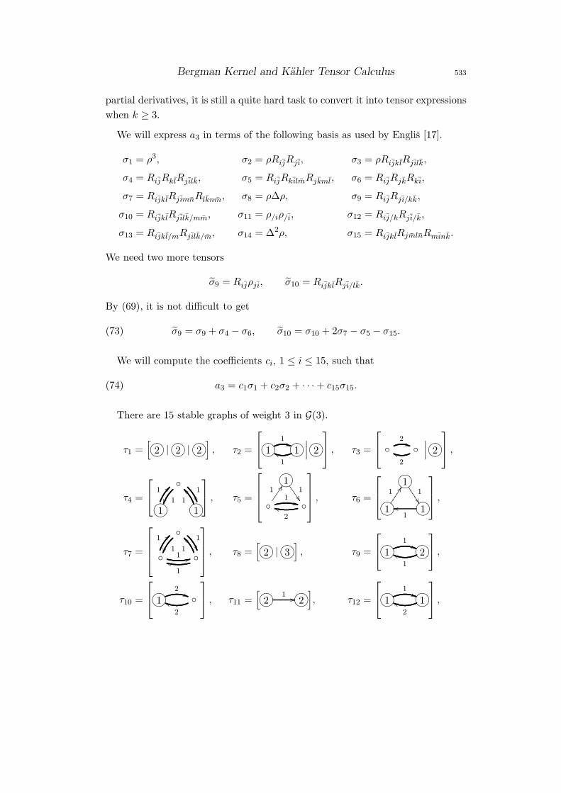
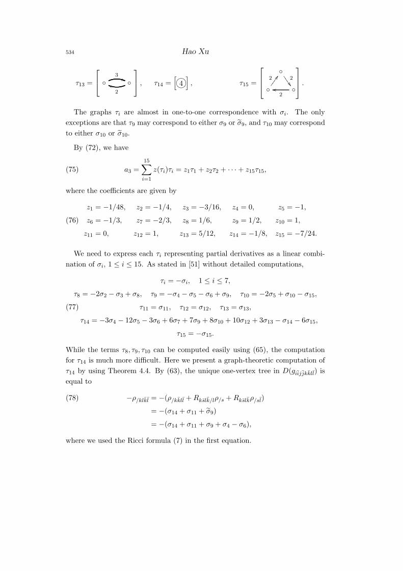
There are 15 stable graphs of weight 3 in G(3).
τ1 =[
765401232 | 765401232 | 765401232], τ2 =
765401231
1((765401231
1
hh
∣∣∣ 765401232
, τ3 =
2((
2
hh
∣∣∣ 765401232
,
τ4 =
11
765401231
1>>
7654012311
`` , τ5 =
76540123115
555
1DD 1
++ 2
kk
, τ6 =
7654012311
444
44
765401231
1EE
7654012311
oo
,
τ7 =
1
1
1==
1 33 1
kk1
aa , τ8 =
[765401232 | 765401233
], τ9 =
765401231
1))765401232
1
ii
,
τ10 =
765401231
2))
2
ii
, τ11 =
[765401232
1 //765401232], τ12 =
765401231
1))765401231
2
ii
,
534 Hao Xu
τ13 =
3))
2
ii
, τ14 =
[765401234], τ15 =
26
666
2DD
2
oo
.
The graphs τi are almost in one-to-one correspondence with σi. The only
exceptions are that τ9 may correspond to either σ9 or σ9, and τ10 may correspond
to either σ10 or σ10.
By (72), we have
(75) a3 =
15∑
i=1
z(τi)τi = z1τ1 + z2τ2 + · · · + z15τ15,
where the coefficients are given by
z1 = −1/48, z2 = −1/4, z3 = −3/16, z4 = 0, z5 = −1,
z6 = −1/3, z7 = −2/3, z8 = 1/6, z9 = 1/2, z10 = 1,(76)
z11 = 0, z12 = 1, z13 = 5/12, z14 = −1/8, z15 = −7/24.
We need to express each τi representing partial derivatives as a linear combi-
nation of σi, 1 ≤ i ≤ 15. As stated in [51] without detailed computations,
τi = −σi, 1 ≤ i ≤ 7,
τ8 = −2σ2 − σ3 + σ8, τ9 = −σ4 − σ5 − σ6 + σ9, τ10 = −2σ5 + σ10 − σ15,
τ11 = σ11, τ12 = σ12, τ13 = σ13,(77)
τ14 = −3σ4 − 12σ5 − 3σ6 + 6σ7 + 7σ9 + 8σ10 + 10σ12 + 3σ13 − σ14 − 6σ15,
τ15 = −σ15.
While the terms τ8, τ9, τ10 can be computed easily using (65), the computation
for τ14 is much more difficult. Here we present a graph-theoretic computation of
τ14 by using Theorem 4.4. By (63), the unique one-vertex tree in D(giijjkkll) is
equal to
−ρ/klkl = −(ρ/kkll +Rkslk/lρ/s +Rkslkρ/sl)(78)
= −(σ14 + σ11 + σ9)
= −(σ14 + σ11 + σ9 + σ4 − σ6),
where we used the Ricci formula (7) in the first equation.
Bergman Kernel and Kahler Tensor Calculus 535
The 48 trees in D(giijjklkl) with at least two vertices are enumerated in Tables
1-6 in Appendix A. Note that each tree T is weighted by (−1)|V (T )|. A tree
is labeled by the dagger symbol † if and only if i, j are contained in a proper
subtree.
From (1), we have
(79) τ14 = D(giijjklkl) = D(−∂klklRiijj) +D(∂klkl(g
mngmijginj)).
Denote by I, II, . . . , IV the sum of trees in the same numbered table such that
i, j are not both contained in a proper subtree. By (62) and (78),
D(−∂klklRiijj) = −(σ14 + σ11 + σ9 + σ4 − σ6) + I + II + III + IV + V + V I
= −(σ14 + σ11 + σ9 + σ4 − σ6) + 2σ9 + (σ11 + 4σ12) + 4σ12
+ (4σ9 + 2σ9 + 4σ10) − (2σ4 + 2σ5 + 2σ6) − (2σ4 + 2σ7)
= −3σ4 − 6σ5 − 3σ6 + 6σ7 + 7σ9 + 4σ10 + 8σ12 − σ14 − 4σ15.
Denote by I ′, II ′, . . . , IV ′ the sum of trees in the same numbered table such
that i, j are contained in a proper subtree. By (61),
D(∂klkl(g
mngmijginj))
= I ′ + II ′ + III ′ + IV ′ + V ′ + V I ′
= (σ10 + σ10) + σ13 + (2σ12 + 2σ13) + 2σ10 − (3σ5 + 2σ7 + σ15) − 2σ5
= −6σ5 + 4σ10 + 2σ12 + 3σ13 − 2σ15.
Adding up the above two identities, we get the desired tensor expression for τ14.
Substituting (77) into (75), we can get the coefficients in (74).
c1 = 1/48, c2 = −1/12, c3 = 1/48, c4 = −1/8, c5 = 0,
c6 = 5/24, c7 = −1/12, c8 = 1/6, c9 = −3/8, c10 = 0,
c11 = 0, c12 = −1/4, c13 = 1/24, c14 = 1/8, c15 = 1/24.
6. Partial and covariant derivatives of functions
For any smooth function f defined on a Kahler manifold, we may derive from
(7) the following well-known identities:
f/α = fα, f/ij = f/ji = fij,
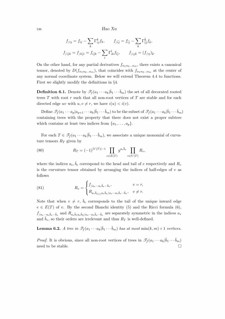
536 Hao Xu
f/ij = fij −∑
k
Γkijfk, f/ij = fij −
∑
k
Γkijfk,
f/ijk = f/kji = fijk −∑
l
Γlikflj, f/ijk = (f/ij)k.
On the other hand, for any partial derivatives fα1α2...αm , there exists a canonical
tensor, denoted by D(fα1α2...αm), that coincides with fα1α2...αm at the center of
any normal coordinate system. Below we will extend Theorem 4.4 to functions.
First we slightly modify the definitions in §4.
Definition 6.1. Denote by Tf (a1 · · · ak|b1 · · · bm) the set of all decorated rooted
trees T with root r such that all non-root vertices of T are stable and for each
directed edge uv with u, v 6= r, we have i(u) < i(v).
Define Tf (a1 · · · ap|ap+1 · · · ak|b1 · · · bm) to be the subset of Tf (a1 · · · ak|b1 · · · bm)
containing trees with the property that there does not exist a proper subtree
which contains at least two indices from a1, . . . , ap.
For each T ∈ Tf (a1 · · · ak|b1 · · · bm), we associate a unique monomial of curva-
ture tensors RT given by
(80) RT = (−1)|V (T )|−1∏
e∈E(T )
gae be
∏
v∈V (T )
Rv,
where the indices ae, be correspond to the head and tail of e respectively and Rv
is the curvature tensor obtained by arranging the indices of half-edges of v as
follows
(81) Rv =
f/a∗···a∗ b∗···b∗ , v = r,
Ra∗ bi(v)a∗ be/a∗···a∗b∗···b∗ , v 6= r.
Note that when v 6= r, be corresponds to the tail of the unique inward edge
e ∈ E(T ) of v. By the second Bianchi identity (5) and the Ricci formula (6),
f/a∗···a∗b∗···b∗ and Ra∗ b1a∗b2/a∗···a∗ b∗···b∗ are separately symmetric in the indices a∗and b∗, so their orders are irrelevant and thus RT is well-defined.
Lemma 6.2. A tree in Tf (a1 · · · ak|b1 · · · bm) has at most min(k,m)+1 vertices.
Proof. It is obvious, since all non-root vertices of trees in Tf (a1 · · · ak|b1 · · · bm)
need to be stable.
Bergman Kernel and Kahler Tensor Calculus 537
Theorem 6.3. Let k ≥ p ≥ 0 and m ≥ 0. Then
(82) D((f/a1···ap
)ap+1···ak b3···bm
)=
∑
T∈Tf (a1···ap|ap+1···ak |b1···bm)
RT .
Proof. Obviously (82) holds when p = k. From (2), we have
(83) (f/a1···ap)ap+1···ak b1···bm
= (f/a1···apap+1)ap+2···ak b1···bm
+
p∑
j=1
(grsgap+1sajf/a1···aj−1raj+1···ap
)ap+2···ak b1···bm.
Then by induction, in the right-hand side of (83), the first term produces trees
with the property that no two of a1, . . . , ap, ap+1 are contained in a proper
subtree, the last term produces trees with the property that aj , ap+1 (1 ≤ j ≤ p)
are contained in a proper subtree. The coefficient of each tree can be determined
by exactly the same argument as in the above proof of (61). So we conclude the
inductive proof of (82).
Corollary 6.4. Let k,m ≥ 0. Then
(84) D(fa1···ak b1···bm) =
∑
T∈Tf (a1···ak |b1···bm)
RT .
Proof. We get the equation by taking p = 0 in (82).
Example 6.5. Let us compute D(fijk). Since there is a one-vertex tree and a
two-vertex tree in Tf (ij | k), by (84), we get
(85) D(fijk) = f/ijk − f/lRikjl.
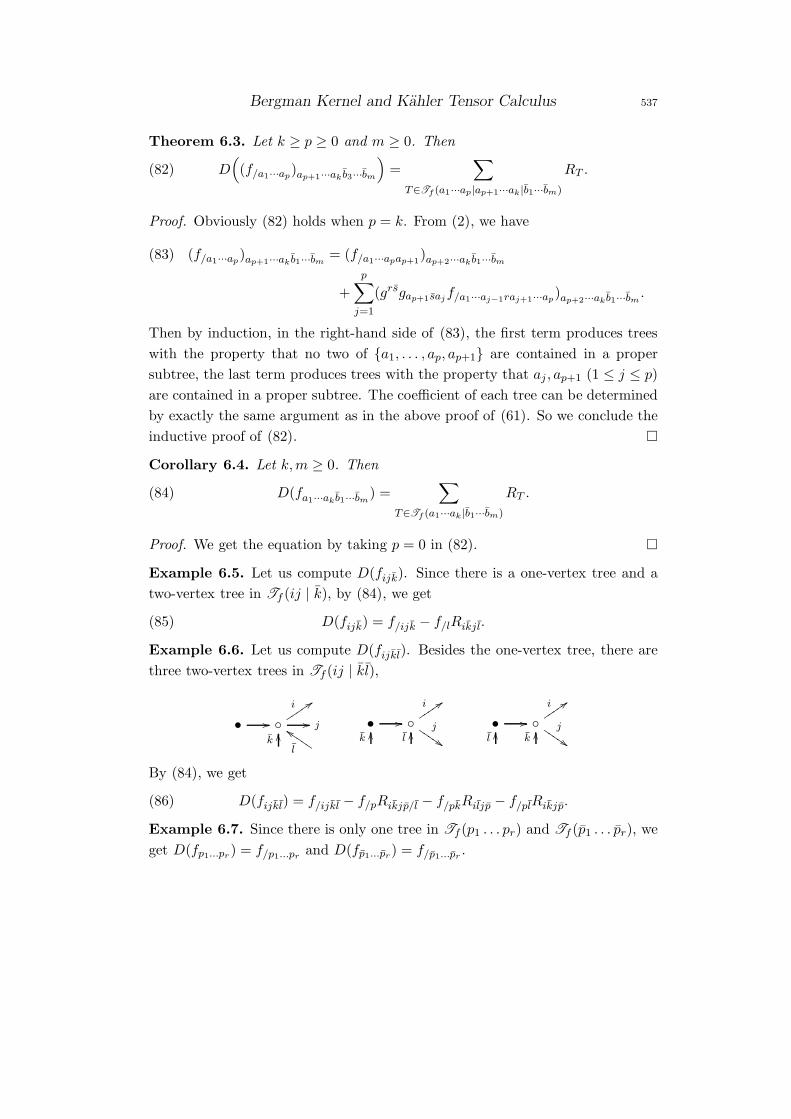
Example 6.6. Let us compute D(fijkl). Besides the one-vertex tree, there are
three two-vertex trees in Tf (ij | kl),
• //
i ::ttttt // jk
OO
l
ddJJJJJ• //
i ::uuuuuj
$$IIIII
kOO
lOO • //
i ::uuuuuj
$$IIIII
lOO
kOO
By (84), we get
(86) D(fijkl) = f/ijkl − f/pRikjp/l − f/pkRiljp − f/plRikjp.
Example 6.7. Since there is only one tree in Tf (p1 . . . pr) and Tf (p1 . . . pr), we
get D(fp1...pr) = f/p1...prand D(fp1...pr) = f/p1...pr
.
538 Hao Xu
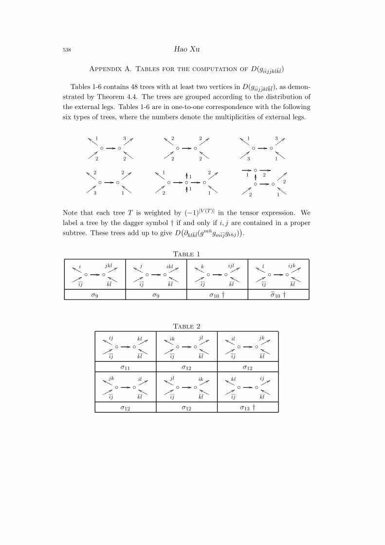
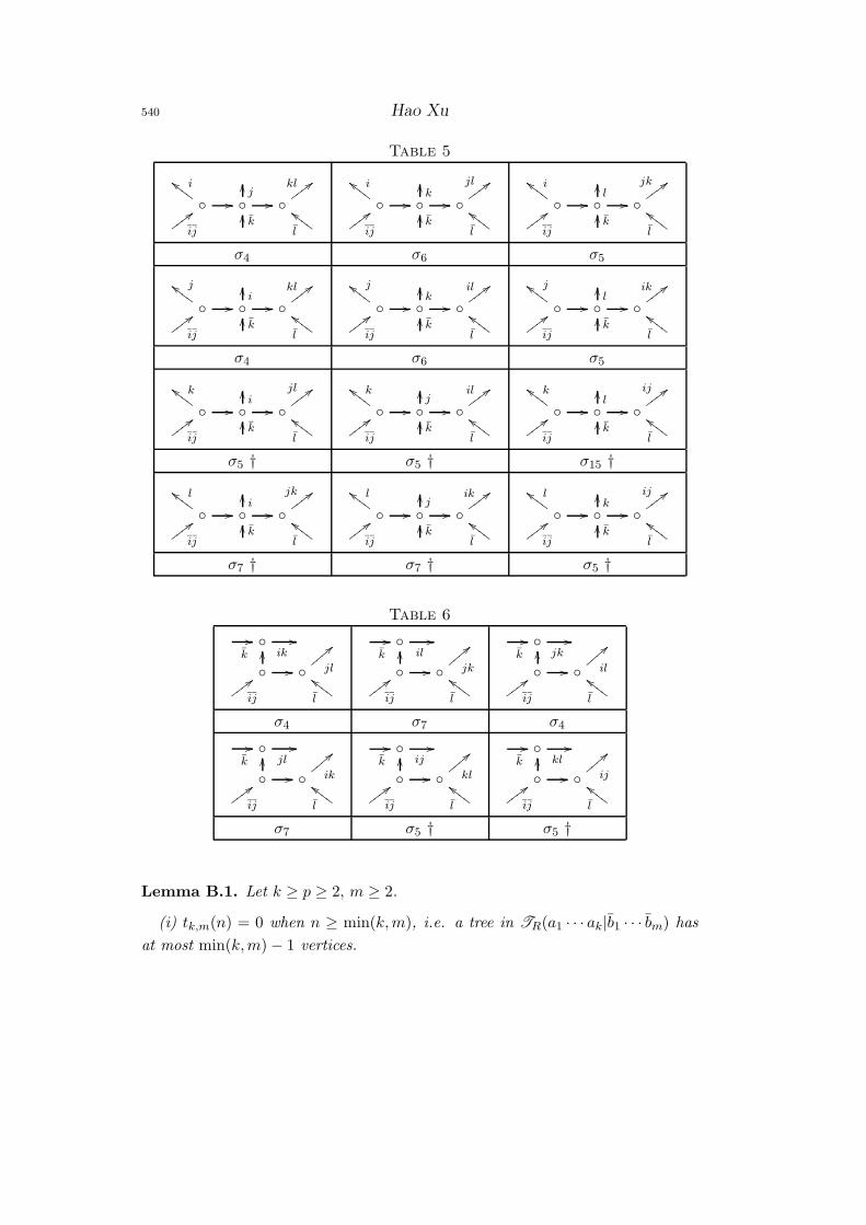
Appendix A. Tables for the computation of D(giijjklkl)
Tables 1-6 contains 48 trees with at least two vertices in D(giijjklkl), as demon-
strated by Theorem 4.4. The trees are grouped according to the distribution of
the external legs. Tables 1-6 are in one-to-one correspondence with the following
six types of trees, where the numbers denote the multiplicities of external legs.
1ccGGGG//
3 ;;wwww
2
;;wwww 2
ccGGGG
2ccGGGG//
2 ;;wwww
2
;;wwww 2
ccGGGG
1ccGGGG//
3 ;;wwww
3
;;wwww 1
ccGGGG
2ccGGGG//
2 ;;wwww
3
;;wwww 1
ccGGGG
1ccGGGG// //
1OO
2 ;;wwww
2
;;wwww 1OO
1
ccGGGG
1//
2//
OO
// 2
==zzzz
2
;;wwww 1
ccGGGG
Note that each tree T is weighted by (−1)|V (T )| in the tensor expression. We
label a tree by the dagger symbol † if and only if i, j are contained in a proper
subtree. These trees add up to give D(∂klkl(g
mngmijginj)).
Table 1
iggNNNN
//
jkl 77pppp
ij
77ppppkl
ggNNNN
jggNNNN//
ikl 77pppp
ij
77ppppkl
ggNNNN
kggNNNN//
ijl 77pppp
ij
77ppppkl
ggNNNN
lggNNNN//
ijk 77pppp
ij
77ppppkl
ggNNNN
σ9 σ9 σ10 † σ10 †
Table 2
ijggNNNN//
kl 77pppp
ij
77ppppkl
ggNNNN
ikggNNNN//
jl 77pppp
ij
77ppppkl
ggNNNN
ilggNNNN//
jk 77pppp
ij
77ppppkl
ggNNNN
σ11 σ12 σ12
jkggNNNN//
il 77pppp
ij
77ppppkl
ggNNNN
jlggNNNN//
ik 77pppp
ij
77ppppkl
ggNNNN
klggNNNN//
ij 77pppp
ij
77ppppkl
ggNNNN
σ12 σ12 σ13 †
Bergman Kernel and Kahler Tensor Calculus 539
Table 3
iggNNNN
//
jkl 77pppp
ijk
77ppppl
ggNNNN
jggNNNN//
ikl 77pppp
ijk
77ppppl
ggNNNN
kggNNNN//
ijl 77pppp
ijk
77ppppl
ggNNNN
lggNNNN//
ijk 77pppp
ijk
77ppppl
ggNNNN
σ12 σ12 σ12 † σ13 †
iggNNNN
//
jkl 77pppp
ij l
77ppppk
ggNNNN
jggNNNN//
ikl 77pppp
ijl
77ppppk
ggNNNN
kggNNNN//
ijl 77pppp
ijl
77ppppk
ggNNNN
lggNNNN//
ijk 77pppp
ij l
77ppppk
ggNNNN
σ12 σ12 σ13 † σ12 †
Table 4
ijggNNNN//
kl 77pppp
ijk
77ppppl
ggNNNN
ikggNNNN//
jl 77pppp
ijk
77ppppl
ggNNNN
ilggNNNN//
jk 77pppp
ijk
77ppppl
ggNNNN
jkggNNNN//
il 77pppp
ijk
77ppppl
ggNNNN
σ9 σ9 σ10 σ9
jlggNNNN//
ik 77pppp
ijk
77ppppl
ggNNNN
klggNNNN//
ij 77pppp
ijk
77ppppl
ggNNNN
ijggNNNN//
kl 77pppp
ijl
77ppppk
ggNNNN
ikggNNNN//
jl 77pppp
ij l
77ppppk
ggNNNN
σ10 σ10 † σ9 σ10
ilggNNNN
//
jk 77pppp
ij l
77ppppk
ggNNNN
jkggNNNN//
il 77pppp
ijl
77ppppk
ggNNNN
jlggNNNN//
ik 77pppp
ijl
77ppppk
ggNNNN
klggNNNN//
ij 77pppp
ij l
77ppppk
ggNNNN
σ9 σ10 σ9 σ10 †
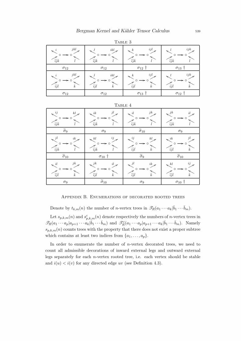
Appendix B. Enumerations of decorated rooted trees
Denote by tk,m(n) the number of n-vertex trees in TR(a1 · · · ak|b1 · · · bm).
Let sp,k,m(n) and scp,k,m(n) denote respectively the numbers of n-vertex trees in
TR(a1 · · · ap|ap+1 · · · ak|b1 · · · bm) and T cR(a1 · · · ap|ap+1 · · · ak|b1 · · · bm). Namely
sp,k,m(n) counts trees with the property that there does not exist a proper subtree
which contains at least two indices from a1, . . . , ap.
In order to enumerate the number of n-vertex decorated trees, we need to
count all admissible decorations of inward external legs and outward external
legs separately for each n-vertex rooted tree, i.e. each vertex should be stable
and i(u) < i(v) for any directed edge uv (see Definition 4.3).
540 Hao Xu
Table 5
iccGGGG// //
jOO
kl ;;wwww
ij
;;wwww kOO
l
ccGGGG
iccGGGG// //
kOO
jl ;;wwww
ij
;;wwww kOO
l
ccGGGG
iccGGGG// //
lOO
jk ;;wwww
ij
;;wwww kOO
l
ccGGGG
σ4 σ6 σ5
jccGGGG// //
iOO
kl ;;wwww
ij
;;wwww kOO
l
ccGGGG
jccGGGG// //
kOO
il ;;wwww
ij
;;wwww kOO
l
ccGGGG
jccGGGG// //
lOO
ik ;;wwww
ij
;;wwww kOO
l
ccGGGG
σ4 σ6 σ5
kccGGGG// //
iOO
jl ;;wwww
ij
;;wwww kOO
l
ccGGGG
kccGGGG// //
jOO
il ;;wwww
ij
;;wwww kOO
l
ccGGGG
kccGGGG// //
lOO
ij ;;wwww
ij
;;wwww kOO
l
ccGGGG
σ5 † σ5 † σ15 †
lccGGGG// //
iOO
jk ;;wwww
ij
;;wwww kOO
l
ccGGGG
lccGGGG// //
jOO
ik ;;wwww
ij
;;wwww kOO
l
ccGGGG
lccGGGG// //
kOO
ij ;;wwww
ij
;;wwww kOO
l
ccGGGG
σ7 † σ7 † σ5 †
Table 6
k
// ik
//
OO
// jl
==zzzz
ij
;;wwwwl
ccGGGG
k
// il
//
OO
// jk
==zzzz
ij
;;wwwwl
ccGGGG
k
// jk
//
OO
// il
==zzzz
ij
;;wwwwl
ccGGGG
σ4 σ7 σ4
k
// jl
//
OO
// ik
==zzzz
ij
;;wwwwl
ccGGGG
k
// ij
//
OO
// kl
==zzzz
ij
;;wwwwl
ccGGGG
k
// kl
//
OO
// ij
==zzzz
ij
;;wwwwl
ccGGGG
σ7 σ5 † σ5 †
Lemma B.1. Let k ≥ p ≥ 2, m ≥ 2.
(i) tk,m(n) = 0 when n ≥ min(k,m), i.e. a tree in TR(a1 · · · ak|b1 · · · bm) has
at most min(k,m) − 1 vertices.
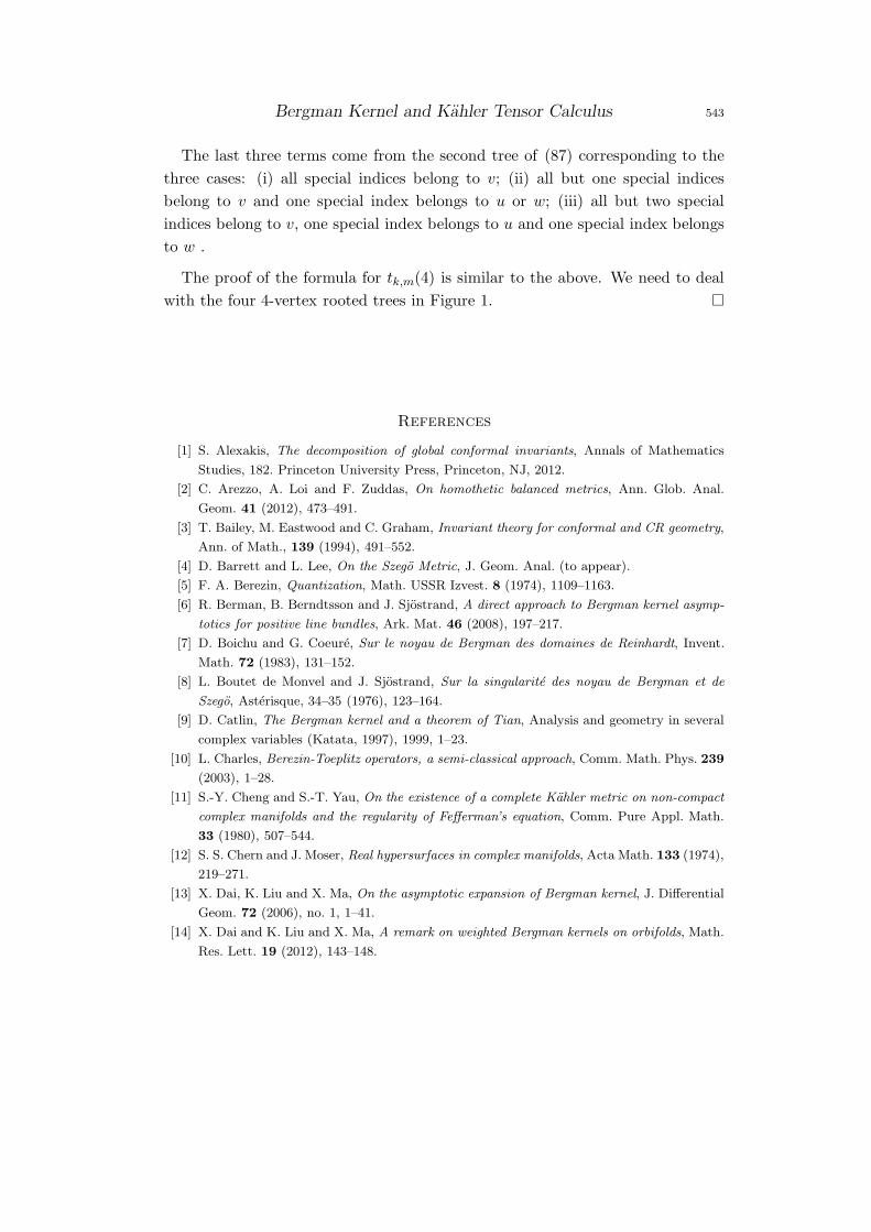
Bergman Kernel and Kahler Tensor Calculus 541
(ii) For 2-vertex trees, we have tk,m(2) = (2k − 2 − k)(2m−2 − 1) and
sp,k,m(2) = ((p + 1)2k−p − k − 1)(2m−2 − 1),
scp,k,m(2) = (2k − (p+ 1)2k−p − 1)(2m−2 − 1).
(ii) For 3-vertex trees, we have
tk,m(3) =
(2 · 3k −
3k
2· 2k − 5 · 2k + k2 + 3k + 4
)(1
183m −
1
42m +
1
2
),
sp,k,m(3) =
(3k−p(p2 + 3p+ 2) − 2k−p−1(3kp + 3k + p2 + 7p+ 8) + k2 + 2k + 2
)
×
(1
183m −
1
42m +
1
2
).
(iii) For 4-vertex trees, we have
tk,m(4) =
(6 · 4k − 3k(4k + 19) + 2k
(7
4k2 +
43
4k + 21
)− (k3 + 4k2 + 9k + 9)
)
×
(1
964m −
1
183m +
1
82m −
1
6
).
Proof. (i) is obvious, since each tree in TR(a1 · · · ak|b1 · · · bm) is stable.
Now we prove (ii). From the unique one 2-vertex tree, we have
tk,m(2) =
k−1∑
i=2
(k
i
)m−2∑
j=1
(m− 2
j
)= (2k − 2 − k)(2m−2 − 1),
sp,k,m(2) =
(k−p∑
i=2
(k − p
i
)+ p
k−p∑
i=1
(k − p
i
))m−2∑
j=1
(m− 2
j
)
=((p + 1)2k−p − k − 1)(2m−2 − 1),
scp,k,m(2) =
p∑
i=2
(p
i
) k−p∑
j=0
(k − p
j
)− 1
m−2∑
j=1
(m− 2
j
)
=(2k − (p+ 1)2k−p − 1)(2m−2 − 1).
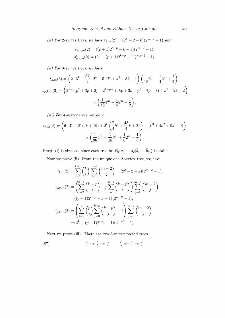
Next we prove (iii). There are two 3-vertex rooted trees
(87) x
// y
// z
u
v
oo // w
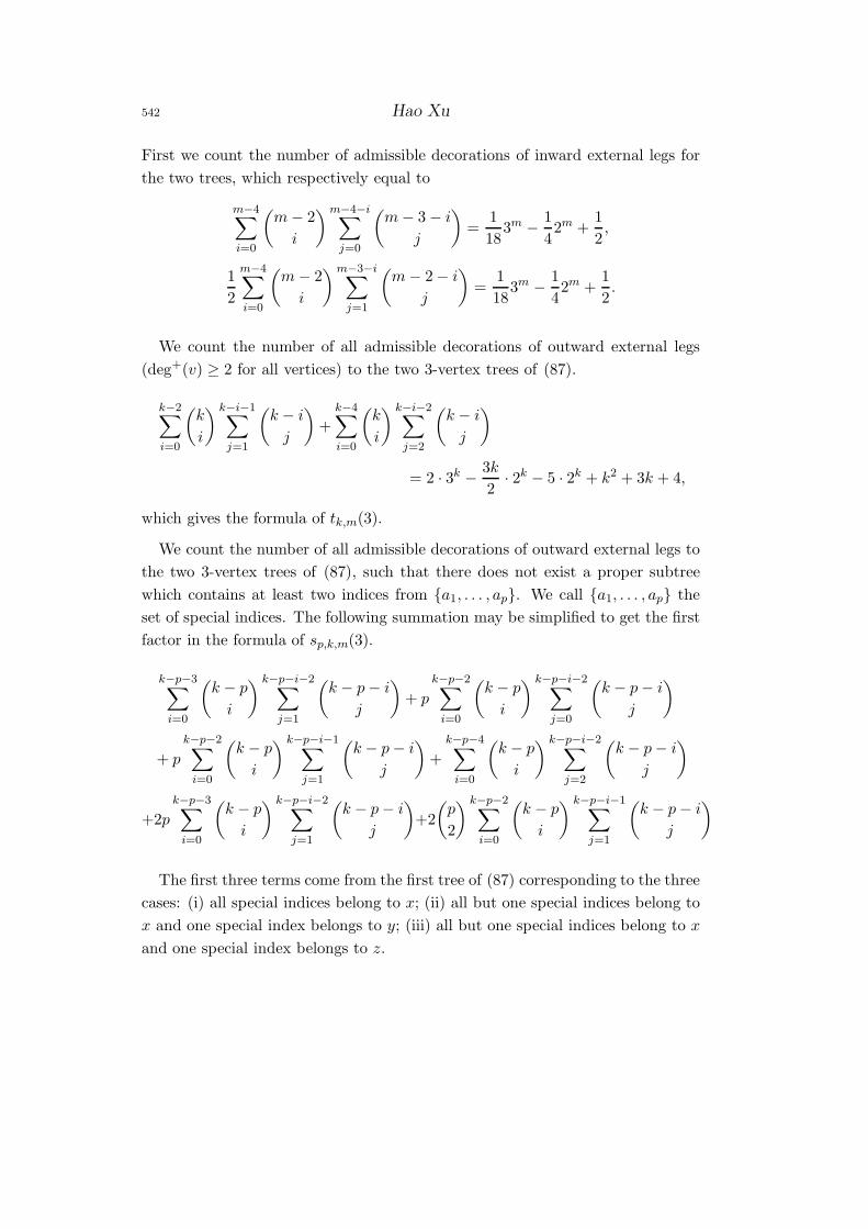
542 Hao Xu
First we count the number of admissible decorations of inward external legs for
the two trees, which respectively equal to
m−4∑
i=0
(m− 2
i
)m−4−i∑
j=0
(m− 3 − i
j
)=
1
183m −
1
42m +
1
2,
1
2
m−4∑
i=0
(m− 2
i
)m−3−i∑
j=1
(m− 2 − i
j
)=
1
183m −
1
42m +
1
2.
We count the number of all admissible decorations of outward external legs
(deg+(v) ≥ 2 for all vertices) to the two 3-vertex trees of (87).
k−2∑
i=0
(k
i
) k−i−1∑
j=1
(k − i
j
)+
k−4∑
i=0
(k
i
) k−i−2∑
j=2
(k − i
j
)
= 2 · 3k −3k
2· 2k − 5 · 2k + k2 + 3k + 4,
which gives the formula of tk,m(3).
We count the number of all admissible decorations of outward external legs to
the two 3-vertex trees of (87), such that there does not exist a proper subtree
which contains at least two indices from a1, . . . , ap. We call a1, . . . , ap the
set of special indices. The following summation may be simplified to get the first
factor in the formula of sp,k,m(3).
k−p−3∑
i=0
(k − p
i
) k−p−i−2∑
j=1
(k − p− i
j
)+ p
k−p−2∑
i=0
(k − p
i
) k−p−i−2∑
j=0
(k − p− i
j
)
+ p
k−p−2∑
i=0
(k − p
i
) k−p−i−1∑
j=1
(k − p− i
j
)+
k−p−4∑
i=0
(k − p
i
) k−p−i−2∑
j=2
(k − p− i
j
)
+2p
k−p−3∑
i=0
(k − p
i
) k−p−i−2∑
j=1
(k − p− i
j
)+2
(p
2
) k−p−2∑
i=0
(k − p
i
) k−p−i−1∑
j=1
(k − p− i
j
)
The first three terms come from the first tree of (87) corresponding to the three
cases: (i) all special indices belong to x; (ii) all but one special indices belong to
x and one special index belongs to y; (iii) all but one special indices belong to x
and one special index belongs to z.
Bergman Kernel and Kahler Tensor Calculus 543
The last three terms come from the second tree of (87) corresponding to the
three cases: (i) all special indices belong to v; (ii) all but one special indices
belong to v and one special index belongs to u or w; (iii) all but two special
indices belong to v, one special index belongs to u and one special index belongs
to w .
The proof of the formula for tk,m(4) is similar to the above. We need to deal
with the four 4-vertex rooted trees in Figure 1.
References
[1] S. Alexakis, The decomposition of global conformal invariants, Annals of Mathematics
Studies, 182. Princeton University Press, Princeton, NJ, 2012.
[2] C. Arezzo, A. Loi and F. Zuddas, On homothetic balanced metrics, Ann. Glob. Anal.
Geom. 41 (2012), 473–491.
[3] T. Bailey, M. Eastwood and C. Graham, Invariant theory for conformal and CR geometry,
Ann. of Math., 139 (1994), 491–552.
[4] D. Barrett and L. Lee, On the Szego Metric, J. Geom. Anal. (to appear).
[5] F. A. Berezin, Quantization, Math. USSR Izvest. 8 (1974), 1109–1163.
[6] R. Berman, B. Berndtsson and J. Sjostrand, A direct approach to Bergman kernel asymp-
totics for positive line bundles, Ark. Mat. 46 (2008), 197–217.
[7] D. Boichu and G. Coeure, Sur le noyau de Bergman des domaines de Reinhardt, Invent.
Math. 72 (1983), 131–152.
[8] L. Boutet de Monvel and J. Sjostrand, Sur la singularite des noyau de Bergman et de
Szego, Asterisque, 34–35 (1976), 123–164.
[9] D. Catlin, The Bergman kernel and a theorem of Tian, Analysis and geometry in several
complex variables (Katata, 1997), 1999, 1–23.
[10] L. Charles, Berezin-Toeplitz operators, a semi-classical approach, Comm. Math. Phys. 239
(2003), 1–28.
[11] S.-Y. Cheng and S.-T. Yau, On the existence of a complete Kahler metric on non-compact
complex manifolds and the regularity of Fefferman’s equation, Comm. Pure Appl. Math.
33 (1980), 507–544.
[12] S. S. Chern and J. Moser, Real hypersurfaces in complex manifolds, Acta Math. 133 (1974),
219–271.
[13] X. Dai, K. Liu and X. Ma, On the asymptotic expansion of Bergman kernel, J. Differential
Geom. 72 (2006), no. 1, 1–41.
[14] X. Dai and K. Liu and X. Ma, A remark on weighted Bergman kernels on orbifolds, Math.
Res. Lett. 19 (2012), 143–148.
544 Hao Xu
[15] S. Donaldson, Scalar curvature and projective embeddings, I, J. Differential Geom. 59
(2001), no. 3, 479–522.
[16] M. Douglas and S. Klevtsov, Bergman Kernel from Path Integral, Comm. Math. Phys.
293 (2010), 205–230.
[17] M. Englis, The asymptotics of a Laplace integral on a Kahler manifold, J. Reine Angew.
Math. 528 (2000), 1–39.
[18] M. Englis, A Forelli-Rudin construction and asymptotics of weighted Bergman kernels, J.
Funct. Anal. 177 (2000), 257–281.
[19] M. Englis and H. Xu, Forelli-Rudin construction and asymptotic expansion of Szego kernel,
preprint.
[20] C. Fefferman, The Bergman kernel and biholomorphic mappings of pseudoconvex domains,
Invent. Math. 26 (1974), 1–65.
[21] C. Fefferman, Monge-Ampere equations, the Bergman kernel and geometry of pseudoconvex
domains, Ann. of Math. 103 (1976), 395–416; Correction, ibid., 104 (1976), 393–394.
[22] C. Fefferman, Parabolic invariant theory in complex analysis, Adv. Math. 31 (1979), 131–
262.
[23] S. Fu and B. Wong, On strictly pseudoconvex domains with Kahler-Einstein Bergman
metrics, Math. Res. Lett. 4 (1997), 697–703.
[24] M. Garcıa-Fernandez, J. Ross, Limits of balanced metrics on vector bundles and polarised
manifolds, arXiv:1111.2819.
[25] C. R. Graham, Scalar boundary invariants and the Bergman kernel, in “Complex Analysis
II”, Lecture Notes in Math., 1276, pp. 108–135, Springer, 1987.
[26] C. R. Graham, Higher asymptotics of the complex Monge-Ampere equation, Compositio
Math. 64 (1987), 133–155.
[27] K. Hirachi, Construction of boundary invariants and the logarithmic singularity of the
Bergman kernel, Ann. of Math. 151 (2000), 151–190.
[28] K. Hirachi, CR invariants of weight 6, Several complex variables (Seoul, 1998), J. Korean
Math. Soc. 37 (2000), 177–191.
[29] K. Hirachi and G. Komatsu, Invariant theory of the Bergman kernel, in “CR-geometry
and overdetermined systems” (Osaka, 1994), 167–220, Adv. Stud. Pure Math., 25, Math.
Soc. Japan, Tokyo, 1997.
[30] K. Hirachi, G. Komatsu and N. Nakazawa, Two methods of determining local invariants
in the Szego kernel, in “Complex Geometry”, Lecture Notes in Pure and Appl. Math.,
143, pp. 77–96, Dekker, 1993.
[31] K. Hirachi, G. Komatsu and N. Nakazawa, CR invariants of weight five in the Bergman
kernel, Adv. Math. 143 (1999), 185–250.
[32] L. Hormander, L2 estimates and existence theorems for the ∂ operator, Acta Math. 113
(1965), 89–152.
[33] C-Y. Hsiao and G. Marinescu, Asymptotics of spectral function of lower energy forms and
Bergman kernel of semi-positive and big line bundles, arXiv:1112.5464.
[34] J. Kamimoto, Newton polyhedra and the Bergman kernel, Math. Z. 246 (2004), 405–440.
Bergman Kernel and Kahler Tensor Calculus 545
[35] A. Karabegov and M. Schlichenmaier, Identification of Berezin-Toeplitz deformation quan-
tization, J. Reine Angew. Math. 540 (2001), 49–76.
[36] M. Kuranishi, The formula for the singularity of Szego kernel. I, J. Korean Math. Soc. 40
(2003), 641–666.
[37] J. Lee and R. Melrose, Boundary behaviour of the complex Monge-Ampere equation, Acta
Math. 148 (1982), 159–192.
[38] V. Liskovec, On a recurrence method of counting graphs with labelled vertices, Soviet Math.
Dokl. 10 (1969), 242–246.
[39] K. Liu, Heat kernel and moduli spaces, Math. Res. Lett. 3 (1996), 743–762.
[40] K. Liu, Heat kernel and moduli spaces II., Math. Res. Lett. 4 (1997), 569–588.
[41] K. Liu, Heat kernels, symplectic geometry, moduli spaces and finite groups., Surv. Differ.
Geom. 5 (1999), 527–542.
[42] C. Liu and Z. Lu, On the asymptotic expansion of Tian-Yau-Zelditch, arixv:1105.0221.
[43] A. Loi, The Tian–Yau–Zelditch asymptotic expansion for real analytic Kahler metrics, Int.
J. Geom. Methods in Modern Phys. 1 (2004), 253–263.
[44] A. Loi, A Laplace integral on a Kahler manifold and Calabi’s diastasis function, Differential
Geom. Appl. 23 (2005), 55–66.
[45] Z. Lu, On the lower order terms of the asymptotic expansion of Tian-Yau-Zelditch, Amer.
J. Math. 122 (2000), no. 2, 235–273.
[46] X. Ma and G. Marinescu, Generalized Bergman kernels on symplectic manifolds, Adv.
Math. 217 (2008), no. 4, 1756–1815.
[47] N. Mok and S.-T. Yau, Completeness of the Kahler-Einstein metric on bounded domains
and the characterization of domains of holomorphy by curvature conditions, The Math-
ematical Heritage of Henri Poincare, Proc. Sympos. Pure Math., 39, Amer. Math. Soc.,
1983, pp. 41–59.
[48] N. Nakazawa, Asymptotic expansion of the Bergman kernel for strictly pseudoconvex com-
plete Reinhardt domains in C2, Osaka J. Math. 31 (1994), 291–329.
[49] J. Ross and R. Thomas, Weighted Bergman kernels on orbifolds, J. Differential Geom. 88
(2011), 87–107.
[50] M. Schlichenmaier, Berezin-Toeplitz Quantization and Star Products for Compact Kahler
Manifolds, arXiv:1202.5927.
[51] H. Xu, A closed formula for the asymptotic expansion of the Bergman kernel, Comm.
Math. Phys. 314 (2012), 555–585.
[52] H. Xu, An explicit formula for the Berezin star product, Lett. Math. Phys. 101 (2012),
239–264.
[53] H. Xu, Weyl invariant polynomial and deformation quantization on Kahler manifolds, J.
Geom. Phys. (to appear).
[54] H. Xu and S.-T. Yau, Trees and tensors on Kahler manifolds, Ann. Global Anal. Geom.
44 (2013), 151–168..
[55] S.-T. Yau, Problem Section, Seminar on Differential geometry (S.-T. Yau, eds.), Ann. of
Math. Studies, vol. 102, Princeton Univ. Press, 1982, pp. 669–706.
[56] S.-T. Yau, Nonlinear analysis in geometry, L’Enseignement Math. 33 (1987), 109–158.
546 Hao Xu
[57] S. Zelditch, Szego kernel and a theorem of Tian, Internat. Math. Res. Notices, 1998, no.
6, 317–331.
[58] S. Zelditch, Survey of the inverse spectral problem, Surv. Differ. Geom. IX (2004) 401–467.
Hao Xu
Center of Mathematical Sciences, Zhejiang University, Hangzhou, Zhejiang 310027,
China;
Department of Mathematics, Harvard University, Cambridge, MA 02138, USA
E-mail: [email protected]
![) and K · f1(1285)! a0(980)ˇ decay: formalism Vertices: f1 K (K 1) K (K).. it1 = igf1C1ϵ ϵ′ gf1 = 7555 MeV, evaluated as the residue at the pole of T = [1 VG] 1V for K K c:c:](https://static.fdocument.org/doc/165x107/5f08d6ad7e708231d423f7ef/-and-k-f11285-a0980-decay-formalism-vertices-f1-k-k-1-k-k-it1-.jpg)


![BIOELECTRO- MAGNETISM - Bioelectromagnetism · Generation of bioelectric signal V. m [mV] 200. 400. 800. 1000-100-50. 0. 50. Time [ms] K + Na + K + K + K + K + K + K + K + K + K +](https://static.fdocument.org/doc/165x107/5ad27ef17f8b9a72118d34d0/bioelectro-magnetism-bi-of-bioelectric-signal-v-m-mv-200-400-800-1000-100-50.jpg)