Master Thesis

bc− βββγγγ Systems and Elliptic Genus

Author:

Vassilis Anagiannis

Main Supervisor:

dr. Miranda Cheng

Second Supervisor:

prof. dr. Jan de Boer

July 26, 2016

Abstract

The ultimate aim of this thesis is to describe the connection between a mathematicalconstruction, known as the chiral de Rham complex, and the nonlinear sigma modelon Calabi-Yau manifolds with N = (2, 2) supersymmetry. To this end, we first pro-vide a detailed review of the bc − βγ systems, which are free conformal field theoriesin 2 dimensions with some unusual characteristics, as compared to the standard freefermions/bosons. Apart from naturally appearing as the Fadeev-Popov gauge fixingghost fields in the BRST quantization of string theory, these systems are also the buildingblocks of the chiral de Rham complex. The latter possesses a topological superconformalalgebra, which resembles the chiral algebra of the A-model, i.e. the topologically twistednonlinear sigma model on Calabi-Yau manifolds with N = (2, 2) supersymmetry. Weexpress the elliptic genus of that model in terms of the geometry of the target manifoldin such a way, so that it becomes manifest that the chiral de Rham complex is essentiallythe infinite volume limit of the A-model, as far as the calculation of the elliptic genus isconcerned. Furthermore, we demonstrate that the chiral de Rham complex provides analternative way of calculating the elliptic genus, namely as the super-Euler characteristicin the sheaf cohomology of the chiral de Rham complex.

Contents

1 Introduction 1

2 The bc− βββγγγ systems 22.1 Equations of motion, OPEs and mode expansions . . . . . . . . . . . . . 22.2 Virasoro field and central charge . . . . . . . . . . . . . . . . . . . . . . . 52.3 U(1) symmetry, bosonization and vacua . . . . . . . . . . . . . . . . . . . 82.4 The bc− βγ systems on the cylinder . . . . . . . . . . . . . . . . . . . . 13

2.4.1 Mode expansions . . . . . . . . . . . . . . . . . . . . . . . . . . . 132.4.2 Virasoro field and ground states . . . . . . . . . . . . . . . . . . . 142.4.3 U(1) charge . . . . . . . . . . . . . . . . . . . . . . . . . . . . . . 17

3 Characters of the bc− βββγγγ systems and Z2 orbifold 183.1 Torus and modular group . . . . . . . . . . . . . . . . . . . . . . . . . . 183.2 Fermi systems . . . . . . . . . . . . . . . . . . . . . . . . . . . . . . . . . 203.3 Bose systems . . . . . . . . . . . . . . . . . . . . . . . . . . . . . . . . . 23

4 BRST quantization of the bosonic string and the Fermi h = 2 system 254.1 Gauge fixing and Weyl anomaly . . . . . . . . . . . . . . . . . . . . . . . 254.2 General BRST procedure . . . . . . . . . . . . . . . . . . . . . . . . . . . 274.3 Ghost ground states and physical states of the bosonic string . . . . . . . 28

5 The chiral de Rham complex 315.1 Vertex Operator Algebras . . . . . . . . . . . . . . . . . . . . . . . . . . 315.2 The topological bc− βγ system . . . . . . . . . . . . . . . . . . . . . . . 325.3 The embedding of the usual algebraic de Rham complex . . . . . . . . . 345.4 Coordinate transformations and morphisms of the SVOAs . . . . . . . . 35

6 Elliptic genus and the chiral de Rham complex 396.1 Twisted nonlinear sigma model and its infinite volume limit . . . . . . . 396.2 The elliptic genus as a geometric index . . . . . . . . . . . . . . . . . . . 456.3 Connection to the chiral de Rham complex . . . . . . . . . . . . . . . . . 53

Appendix 58A Weight calculation for the cylinder ground states . . . . . . . . . . . . . . 58B Difference between orderings in terms of fields . . . . . . . . . . . . . . . 60C Jacobi theta functions . . . . . . . . . . . . . . . . . . . . . . . . . . . . 61

References 62

1 Introduction

This is a Master’s thesis, written as part of the Theoretical Physics track of the Physicsand Astronomy Master’s program of the University of Amsterdam (2015-2016). Its mainfocus revolves around the so-called bc − βγ systems, their role in two-dimensional con-formal field theory, and especially their connection to the elliptic genus of the nonlinearsigma model on Calabi-Yau manifolds with N = (2, 2) supersymmetry.

The bc−βγ systems are free, massless chiral theories with a first order action, whichis build from two different fields. This sets them apart from free theories like the masslessboson or fermion, and gives them unique and interesting characteristics. They can beused, for example, to increase our options when making free field realizations of affinealgebras. Possibly their most common appearance in CFT2 though, is in the context ofthe BRST quantization in string theory, where they have the role of ghosts, naturallyappearing upon fixing the gauge in the worldsheet of the string, using the Faddeev-Popovmethod. The first part of this thesis (Sections 2 to 4) is about the above features.

Yet another occurrence of the bc − βγ systems is in the so-called chiral de Rhamcomplex, a sheaf of supersymmetric vertex operator algebras over a complex manifoldM, first developed by Malikov et al. in [17]. It is notable that this theory features achiral N = 2 topological superconformal algebra, the same one that is present in thechiral part of Witten’s A-model. The latter, developed in [23], is a certain ”truncated”version of the nonlinear sigma model with N = (2, 2) supersymmetry on a Calabi-Yaumanifold M. Furthermore, the A-model is topological, i.e. it does not depend on thetarget manifold metric. Since both the chiral de Rham complex and the A-model sharethe same topological character, they could, in principle, both be used to calculate theelliptic genus of M, which is a known topological quantity. The second part of this thesis(Sections 5 and 6) serves to make the above relation more clear, also based on works byKapustin and Borisov, in [28] and [21] respectively. In the latter work, the elliptic genuswas defined in the sheaf cohomology of the chiral de Rham complex, while in the formera more explicit relation between a certain resolution of the chiral de Rham complex andthe infinite volume limit of the twisted sigma model, another “truncated” version of thenonlinear sigma model that is closely related to the A-model, was shown.

The thesis is structured as follows: Section 2 describes the bc − βγ systems in de-tail, both on the complex plane and on the cylinder, including features like the chargeasymmetry and the infinite number of plane vacua. Section 3 includes calculations ofcertain genus-one characters of these systems, as well as a Z2 orbifold version of them,closely related to the elliptic genus. Section 4 contains some basic details on the BRSTquantization of the bosonic sting, where the bc−βγ systems appear as ghosts. Section 5introduces and describes important features of the chiral de Rham complex, along withbasic notions of vertex operator algebras. Finally, Section 6 makes the connection be-tween the chiral de Rham complex and the elliptic genus of the nonlinear sigma model,including a detailed geometrical expression for the elliptic genus in the infinite volumelimit of the latter as well. The reader would be more comfortable reading through thefollowing text with some basic knowledge of QFT/CFT, bosonic string theory, and a bitof complex geometry/topology.

Last but not least, I would like to thank my supervisor Miranda Cheng for herguidance and enlightening counsel during the writing of this thesis. I would also like tothank Jan de Boer, Francesca Ferrari, Sam van Leuven and Mikola Schlottke for helpfuland insightful discussions. This thesis was financially supported, in part, by the LatsisFoundation scholarship.

1

2 The bc− βββγγγ systems

2.1 Equations of motion, OPEs and mode expansions

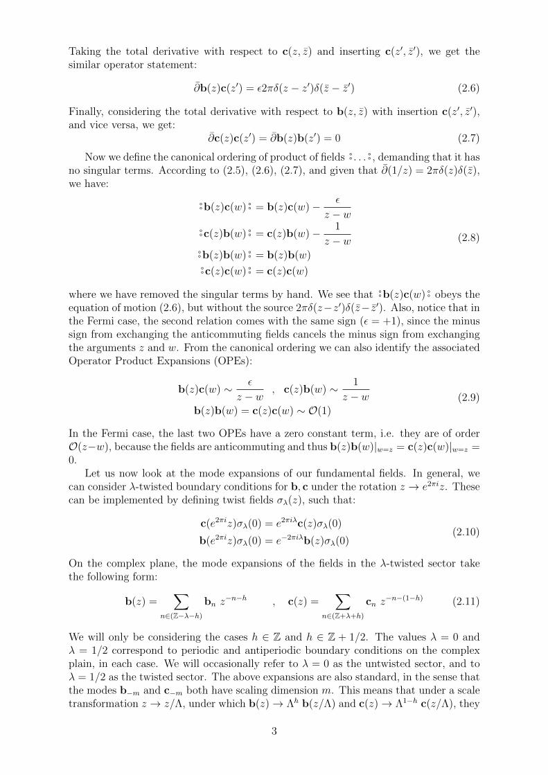
As mentioned in the introduction, the bc − βγ systems are a family of free two-dimensional chiral CFTs, that are described by a first order action. In local complexcoordinates, this action has the general form:

S =1

2π

∫Σ

d2z b∂c (2.1)

where ∂ ≡ ∂∂z

and d2z = dzdz. We will be mainly considering the complex plain1 (genuszero) as the worldsheet Σ, instead of a general Riemann surface of higher genus. All thelocal expressions will be valid, however, in all cases. Looking at S, we distinguish twocases, depending on which statistics the fields b, c obey. We will be using the followingnotation:

b = b, c = c, ε = +1 (Fermi)

b = β, c = γ, ε = −1 (Bose)

We will see that both cases share many common features, but also have some significantdifferences. Thus, we will be treating them in parallel whenever possible, using the signdifference ε to distinguish between them. The two fundamental fields b, c are primary,and they have conformal weights (hb, 0) and (hc, 0), with:

hb ≡ h , hc ≡ 1− h (2.2)

Their weights are of course such, so that S is dimensionless. Indeed, the weight of theLagrangian b∂c is (h + 1 − h, 1) = (1, 1), while that of d2z is (−1,−1), leading totheir cancellation in S. From now on, when we refer to weight we will mean the chiral(left-moving) weight.

The equations of motion can easily be obtained from the (Euclidean) path integralformalism. Using the fact that, at a general point (z, z), a total derivative inside thepath integral gives zero, we have:

0 =

∫DbDc

δ

δb(z, z)

[e−S · · ·

]= − 1

2π

∫DbDc ∂c(z, z) e−S · · · ⇒ 〈∂c(z, z) · · · 〉 = 0 (2.3)

where the dots indicate any insertions that are not at (z, z). We can think of theseinsertions as preparing arbitrary initial and final states, which implies that the aboveresult can be written as an operator statement for the space of states:

∂c(z, z) = 0 ⇒ c(z, z) = c(z) (2.4)

This equation of motion is consistent with our statement that c is chiral (holomorphic).By taking the derivative with respect to c(z, z) in the path integral, we similarly getthat b(z, z) = b(z). The more interesting equations of motion follow from puttingan insertion at a point (z′, z′), which can now take the value (z, z), inside the totalderivative. Using the same arguments as before, as well as that the fields are chiral, weget:

0 =

∫DbDc

δ

δb(z, z)

[b(z′, z′)e−S · · ·

]=

=

∫DbDc

[δ2(z − z′, z − z′)− 1

2π∂c(z)b(z′)

]e−S · · · ⇒

⇒ ∂c(z)b(z′) = 2πδ(z − z′)δ(z − z′)

(2.5)

1or the Riemann sphere, if we want the worldsheet to be compact

2

Taking the total derivative with respect to c(z, z) and inserting c(z′, z′), we get thesimilar operator statement:

∂b(z)c(z′) = ε2πδ(z − z′)δ(z − z′) (2.6)

Finally, considering the total derivative with respect to b(z, z) with insertion c(z′, z′),and vice versa, we get:

∂c(z)c(z′) = ∂b(z)b(z′) = 0 (2.7)

Now we define the canonical ordering of product of fieldsaa . . . aa , demanding that it has

no singular terms. According to (2.5), (2.6), (2.7), and given that ∂(1/z) = 2πδ(z)δ(z),we have: aab(z)c(w)

aa = b(z)c(w)− ε

z − waac(z)b(w)aa = c(z)b(w)− 1

z − waab(z)b(w)aa = b(z)b(w)aac(z)c(w)aa = c(z)c(w)

(2.8)

where we have removed the singular terms by hand. We see thataab(z)c(w)

aa obeys theequation of motion (2.6), but without the source 2πδ(z−z′)δ(z− z′). Also, notice that inthe Fermi case, the second relation comes with the same sign (ε = +1), since the minussign from exchanging the anticommuting fields cancels the minus sign from exchangingthe arguments z and w. From the canonical ordering we can also identify the associatedOperator Product Expansions (OPEs):

b(z)c(w) ∼ ε

z − w, c(z)b(w) ∼ 1

z − wb(z)b(w) = c(z)c(w) ∼ O(1)

(2.9)

In the Fermi case, the last two OPEs have a zero constant term, i.e. they are of orderO(z−w), because the fields are anticommuting and thus b(z)b(w)|w=z = c(z)c(w)|w=z =0.

Let us now look at the mode expansions of our fundamental fields. In general, wecan consider λ-twisted boundary conditions for b, c under the rotation z → e2πiz. Thesecan be implemented by defining twist fields σλ(z), such that:

c(e2πiz)σλ(0) = e2πiλc(z)σλ(0)

b(e2πiz)σλ(0) = e−2πiλb(z)σλ(0)(2.10)

On the complex plane, the mode expansions of the fields in the λ-twisted sector takethe following form:

b(z) =∑

n∈(Z−λ−h)

bn z−n−h , c(z) =

∑n∈(Z+λ+h)

cn z−n−(1−h) (2.11)

We will only be considering the cases h ∈ Z and h ∈ Z + 1/2. The values λ = 0 andλ = 1/2 correspond to periodic and antiperiodic boundary conditions on the complexplain, in each case. We will occasionally refer to λ = 0 as the untwisted sector, and toλ = 1/2 as the twisted sector. The above expansions are also standard, in the sense thatthe modes b−m and c−m both have scaling dimension m. This means that under a scaletransformation z → z/Λ, under which b(z)→ Λh b(z/Λ) and c(z)→ Λ1−h c(z/Λ), they

3

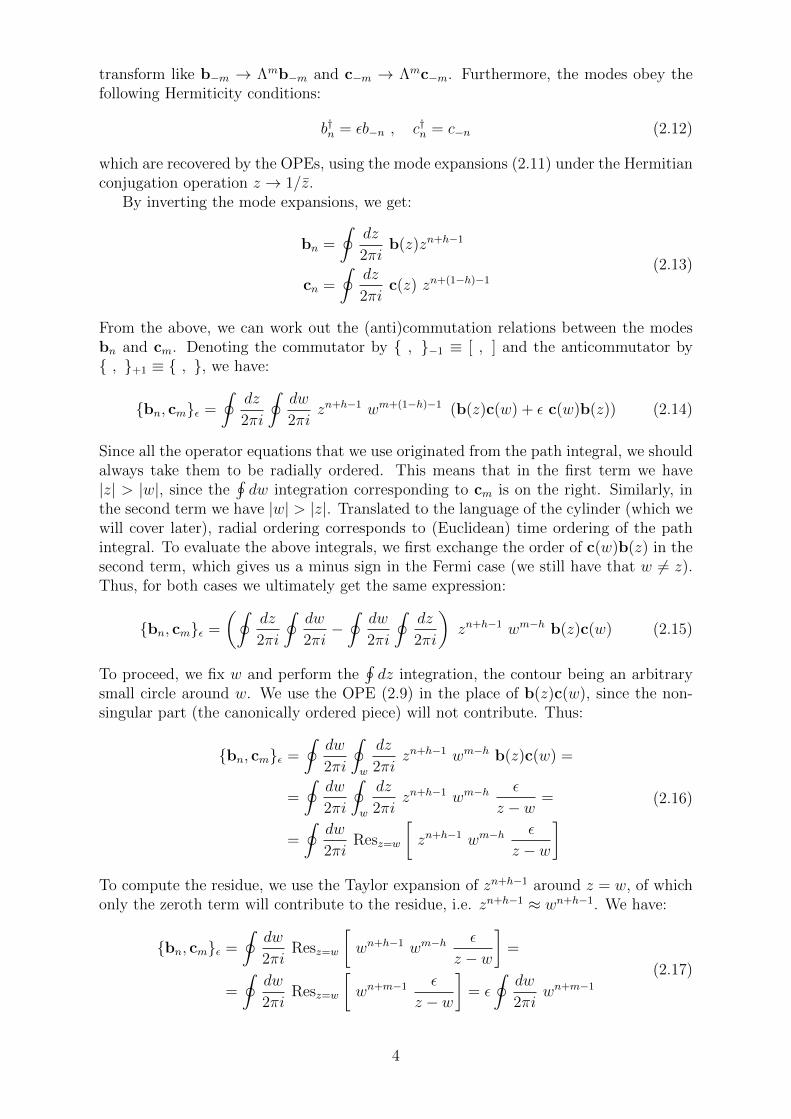
transform like b−m → Λmb−m and c−m → Λmc−m. Furthermore, the modes obey thefollowing Hermiticity conditions:

b†n = εb−n , c†n = c−n (2.12)

which are recovered by the OPEs, using the mode expansions (2.11) under the Hermitianconjugation operation z → 1/z.

By inverting the mode expansions, we get:

bn =

∮dz

2πib(z)zn+h−1

cn =

∮dz

2πic(z) zn+(1−h)−1

(2.13)

From the above, we can work out the (anti)commutation relations between the modesbn and cm. Denoting the commutator by , −1 ≡ [ , ] and the anticommutator by , +1 ≡ , , we have:

bn, cmε =

∮dz

2πi

∮dw

2πizn+h−1 wm+(1−h)−1 (b(z)c(w) + ε c(w)b(z)) (2.14)

Since all the operator equations that we use originated from the path integral, we shouldalways take them to be radially ordered. This means that in the first term we have|z| > |w|, since the

∮dw integration corresponding to cm is on the right. Similarly, in

the second term we have |w| > |z|. Translated to the language of the cylinder (which wewill cover later), radial ordering corresponds to (Euclidean) time ordering of the pathintegral. To evaluate the above integrals, we first exchange the order of c(w)b(z) in thesecond term, which gives us a minus sign in the Fermi case (we still have that w 6= z).Thus, for both cases we ultimately get the same expression:

bn, cmε =

(∮dz

2πi

∮dw

2πi−∮

dw

2πi

∮dz

2πi

)zn+h−1 wm−h b(z)c(w) (2.15)

To proceed, we fix w and perform the∮dz integration, the contour being an arbitrary

small circle around w. We use the OPE (2.9) in the place of b(z)c(w), since the non-singular part (the canonically ordered piece) will not contribute. Thus:

bn, cmε =

∮dw

2πi

∮w

dz

2πizn+h−1 wm−h b(z)c(w) =

=

∮dw

2πi

∮w

dz

2πizn+h−1 wm−h

ε

z − w=

=

∮dw

2πiResz=w

[zn+h−1 wm−h

ε

z − w

] (2.16)

To compute the residue, we use the Taylor expansion of zn+h−1 around z = w, of whichonly the zeroth term will contribute to the residue, i.e. zn+h−1 ≈ wn+h−1. We have:

bn, cmε =

∮dw

2πiResz=w

[wn+h−1 wm−h

ε

z − w

]=

=

∮dw

2πiResz=w

[wn+m−1 ε

z − w

]= ε

∮dw

2πiwn+m−1

(2.17)

4

Thus, the final result for the (anti)commutation relations between the modes bn and cmis:

bn, cmε ≡ bncm + εcmbn = εδn+m,0 (2.18)

This holds, of course, for all cases in (2.11).According to the State-Operator Map, which constitutes an essential feature of two-

dimensional CFTs, states of the quantum theory can be viewed as asymptotic states,created by the action of corresponding local operators (fields) on the SL(2,R)2 invariantvacuum |0〉, at the origin z → 0. The requirement that these states are well-definedimposes, in turn, some conditions for the action of the modes of the associated fieldson the vacuum. In the present case, the states created by the fundamental fields, i.e.|b〉 ≡ limz→0 b(z)|0〉 and |c〉 ≡ limz→0 c(z)|0〉, are well-defined in the SL(2,R) invariantvacuum only if:

bn|0〉 = 0 ∀ n ≥ 1− hcn|0〉 = 0 ∀ n ≥ h

(2.19)

so that we have |b〉 = b−h|0〉 and |c〉 = ch−1|0〉 (the rest of the terms vanish at z → 0).These are the highest weight conditions for the fields b, c on the SL(2,R) invariantvacuum. If higher modes didn’t annihilate the vacuum, then there would exist divergentterms at z → 0, and the states would not be well-defined. This is in full compatibilitywith the canonical ordering; a canonically ordered product is a well-defined field thatcreates well-defined states, which is ensured by putting the modes that annihilate thevacuum to the right. The associated out-states, created by local operators at 1/z → 0,are a little trickier to define for the bc− βγ systems, and we will deal with this issue abit later.

2.2 Virasoro field and central charge

The energy-momentum tensor T (z) (Virasoro field) is the conserved current underglobal translations. It also shows up in all conformal transformations δz = α(z), since theassociated conserved current is nothing but α(z)T (z). For an infinitesimal translationz → z + η, the variation of the action will have the general form:

δS = −∫d2z T (z) ∂η (2.20)

which is trivially zero for constant η. To compute T (z) via Nother’s theorem, we firstpromote η to η(z, z), in the above expression. If the equations of motion are obeyed,the action must be stationary under any variation η(z, z), which is possible only when∂T (z) = 0, i.e. T (z) is conserved3 (after performing integration by parts). This comesfrom the general conservation equation ∂αT

αβ = 0, where T zz ∼ Tzz = T (z) when welower the indices, since the metric on the plane is off-diagonal. Also, the mixed com-ponents T zz, T zz are zero because of the tracelessness of the energy-momentum tensor,originating from classical conformal invariance. Since b, c are primary fields, we knowhow they transform under δz = η(z, z):

δb = [η∂ + h(∂η)]b

δc = [η∂ + (1− h)(∂η)]c(2.21)

2SL(2,R), or more correctly PSL(2,R) = SL(2,R)/Z2, is the group generated globally by the Virasoromodes L0, L±1, which we will encounter later

3note that a conserved current is holomorphic, as is the case always in CFT2

5

where we will write η in the place of η(z, z) for brevity. Using these relations, we maynow vary the action, in order to match it with expression (2.20) and identify the Virasorofield:

δS = δ

(∫d2z b∂c

)=

∫δ(d2z) b∂c +

∫d2z

[δ(b∂c)

δbδb− εδ(b∂c)

δ(∂c)δ(∂c)

](2.22)

Note that the measure is also subject to the transformation η(z, z), and that there isan extra sign for the Fermi case in the last term, due to the Grassmann chain rule. Asmentioned earlier, we want to perform the above calculation on-shell, since we want itto vanish for any variation. Thus, we can use the equations of motion while evaluatingit, which is convenient since one of them is ∂c = 0, leading to many terms droppingout, including the first two terms in the above expression. Furthermore, the derivativewith respect to ∂c gives us an extra minus sign for the Fermi case, since we have toanticommute it past b, ultimately canceling the initial sign. Proceeding, we have:

δS = (−ε)2

∫d2z b ∂(δc) =

∫d2z b ∂[(η∂ + (1− h)∂η)c] =

=

∫d2z [b(∂η)∂c + bη(∂∂c) + (1− h)b(∂∂η)c + (1− h)b(∂η)∂c] =

=

∫d2z [b(∂η)∂c + (1− h)∂(b(∂η)c)− (1− h)∂b(∂η)c− (1− h)b(∂η)∂c] =

= −∫d2z [(1− h)(∂b)c− hb(∂c)] ∂η

(2.23)

where we did integration by parts and dropped the total derivative term. Comparingwith (2.20), we identify the Virasoro fields as:

T (z) = (1− h)aa(∂b)c

aa −h aab(∂c)aa (2.24)

where we have used canonical ordering to make sense of T (z) as a well-defined field inthe quantum case, since the above calculation was classical. It is straightforward tocheck that this expression gives the correct OPEs with the primary fields b, c. From theOPE T (z)T (w), we can also read off the central charge cbc of the bc system:

T (z)T (w) ∼ cbc/2

(z − w)4+

2T (w)

(z − w)2+∂T (w)

z − w(2.25)

withcbc = −2ε(6h2 − 6h+ 1) (2.26)

The central charge changes signs, as a function of h, at the points 12

(1± 1√

3

). We will

be focusing only on the cases where h is either an integer or a half-integer. For laterconvenience, we also define the following quantity:

Q ≡ ε(1− 2h) = ε(hc − hb) (2.27)

This is nothing more than the difference between the weights of the two fields, with theappropriate sign for each of the two cases. In terms of Q, the central charge takes theform:

cbc = ε(1− 3Q2) (2.28)

From (2.25), we also verify that the Virasoro field is a quasi-primary field of weight2. It has the following mode expansion:

T (z) =∑k∈Z

Lk z−k−2 (2.29)

6

The mode Lk is the conserved charge under the conformal transformation δz = ηk(z) ≡ηzk+1, as we can deduce from

∮dz ηk(z)T (z) = Lk. We can express the mode Lk in

terms of modes of the fields b, c by starting from (2.24) and using the expansions (2.11):

T (z) = (1− h)aa(∂b)c

aa −h aab(∂c)aa= (1− h)

aa(∂∑n

bnz−n−h

)∑m

cmz−m−z+h aa −

− h aa∑n

bnz−n−h

(∂∑m

cmz−m−1+h

) aa= (1− h)aa∑n,m

(−n− h)bncmz−n−m−2 aa −

− h aa∑n,m

(−m− 1 + h)bncmz−n−m−2 aa= (1− h)

∑n,m

(−n− h)aabncm aa z−n−m−2−

− h∑n,m

(−m− 1 + h)aabncm aa z−n−m−2

(2.30)

Setting m+ n = k, and noticing that k ∈ Z regardless the sector, we get:

T (z) =∑k∈Z

[(1− h)

∑n

aabnck−n aa (−n− h)z−k−2−

−h∑n

aabnck−n aa (−k + n− 1 + h)z−k−2

](2.29)===⇒

(2.29)===⇒ Lk = (1− h)

∑n

aabnck−n aa (−n− h)− h∑n

aabnck−n aa (−k + n− 1 + h) =

=∑n

[(1− h)(−n− h)− h(−k + n− 1 + h)]aabnck−n aa ⇒

⇒ Lk =∑n

(kh− n)aabnck−n aa

(2.31)

Using the highest weight conditions (2.19) to express the canonical ordering explicitly,we have that:

Lk =∑n

(kh− n)aabnck−n aa= ∑

n≤−h

(kh− n) bnck−n − ε∑

n≥−h+1

(kh− n) ck−nbn (2.32)

Just to verify that this ordering ensures that T (z) is a well-defined field, we considerLk|0〉, which must be zero for k ≥ −1. Indeed, the second sum in Lk|0〉 drops out, sincebn|0〉 = 0 for n ≥ −h+ 1 (using the above expression). The first sum also drops out fork > −1, since (k − n) ≥ (k + h) ≥ h and ck−n|0〉 = 0 for (k − n) ≥ h. Finally, for theremaining case k = −1, the mode c−1−n is not an annihilator for n = −h, but the factor(kh − n) in front vanishes, so we also get L−1|0〉 = 0, as we expected for the SL(2,R)invariant vacuum, since L−1 belongs to the generators of the global SL(2,R) symmetrygroup.

The zero Virasoro mode L0 is of special interest, because it has the role of the Hamil-tonian, i.e. the conserved charge under radial scalings (dilatations), which correspondto time translations on the cylinder4. It induces a Z-grading on the space of states,i.e. H = ⊕m∈ZHm, with Hm being the eigenspace of states with eigenvalue m underL0. This eigenvalue is identified with the conformal weight of the respective eigenstate.Finally, in terms of the b, c fields, the zero mode reads:

L0 =∑n

(−n)aabnc−n aa= ∑

n≤−h

(−n) bnc−n − ε∑

n≥−h+1

(−n) c−nbn (2.33)

4the dilatation is generated by L0+L0 in a general non-chiral theory, where L0 is the antiholomorphiczero Virasoro mode

7

2.3 U(1) symmetry, bosonization and vacua

Apart from conformal invariance, the action (2.1) enjoys an additional U(1) symmetry.It is invariant under the global transformation (b → e−iηb, c → eiηc) (with η aconstant). The infinitesimal version of this transformation is (δb = −iηb, δc = iηc),and through Nother’s procedure, after promoting η to η(z), we obtain the U(1) current:

J(z) = − aabcaa (2.34)

This is a weight 1 field, and after performing calculations akin to those for the Virasorofield, we get the mode expansion:

J(z) =∑k∈Z

Jk z−k−1 , Jk = −

∑n

aabnck−n aa (2.35)

In radial quantization on the complex plane, the contour integral∮dz maps to the

integral around spacial slices on the (more physically relevant) cylinder, so the associatedcharge5 is given by:

N ≡ 1

2πi

∮dz J(z) =

1

2πi

∮dz∑k

Jk z−k−1 = J0 ⇒

⇒ N = J0 = −∑n

aabnc−n aa (2.36)

It is straightforward to show that [N,bn] = −bn and [N, cn] = +cn. This means thatN counts the number of c excitations minus the number of b excitations, symbolicallydenoted as N = #c−#b. Also, using a similar contour integration as in (2.15), we canshow that [L0, N ] = 0, meaning that the space of states is also Z-graded by the U(1)charge, in addition to the Z-grading induced by L0. Thus, we can build a Fock space byacting with the raising operators bn≤−h, cn≤h−1 on the vacuum |0〉. The fact that thecharges of b, c are −1 and +1 respectively, is also manifest in the following OPEs:

J(z)b(w) ∼ − b(w)

z − w, J(z)c(w) ∼ c(w)

z − w, J(z)J(w) ∼ ε

(z − w)2(2.37)

It is now very important that J(z) is not, in general, a primary field. This is evidentfrom its OPE with the Virasoro field:

T (z)J(w) ∼ Q

(z − w)3+

J(w)

(z − w)2+∂J(w)

z − w(2.38)

The extra term that appears is proportional to the difference Q between the weights ofb and c, and it makes J(w) transform under conformal transformations like:

δJ(w) =

[−ε(w)∂w − (∂wε(w))− Q

2∂2w

]J(w) (2.39)

The only case for which J(w) transforms like a primary field is when Q = 0⇔ h = 1/2.The OPE (2.38) also implies that J(z) is not really conserved, but it has an anomaly.

For a general compact Riemann surface of worldsheet metric g, it can be shown (cf. [1])that:

∂J(z) =1

8εQ√gR (2.40)

5which is conserved under (Euclidean) time evolution on the cylinder and under radial evolution(dilatation) on the plane

8

where R is the Ricci scalar of the worldsheet. Integrating this anomaly results in anindex, which enumerates the zero modes Nc of c minus the zero modes Nb of b:

Nc −Nb = εQ(g − 1) = (1− 2h)(g − 1) (2.41)

where g is the genus of the worldsheet and we have used the Gauss-Bonnet theorem,which states that the integral over a compact two-dimensional manifold of the Ricciscalar is equal to the Euler characteristic χ = 2(1− g) of the manifold (modulo factorsof 2π). This index is a global (topological) characteristic of the worldsheet itself, whereasQ is a local feature of the theory, whose meaning will become apparent shortly.

From (2.38) we can also read off the anomalous commutation relations between modesof the Virasoro field and the U(1) current:

[Ln, Jm] = −mJm+n +1

2Qm(m+ 1)δm+n,0 (2.42)

This implies that J(z) transforms covariantly under dilatations (L0) and translations(L−1), but not so under special conformal transformations (L1). Instead, we have that:

[L1, J−1] = J0 +Q (2.43)

If we take the Hermitian adjoint of the above commutator we can calculate the so-calledcharge asymmetry of our theory:

J†0 +Q = [L1, J−1]† = [L−1, J1] = −J0 ⇒ J†0 = −(J0 +Q) (2.44)

whereas for the rest of the modes we simply have that J†n = −J−n ∀ n 6= 0.The charge asymmetry has very important ramifications when calculating expecta-

tion values. If Op is an operator that has charge equal to p under J0, i.e. [J0, Op] = pOp,and |q〉 is similarly a state with charge q, then we have:

p〈q′|Op|q〉 = 〈q′|[J0, Op]|q〉 = 〈q′|J0Op −OpJ0|q〉 = 〈q′|(−J†0 −Q)Op −OpJ0|q〉 =

= −(q′ +Q+ q)〈q′|Op|q〉(2.45)

where J†0 acts on the left and J0 on the right. We see that if we want to have a non-vanishing expectation value between the states 〈q′| and |q〉, we need to insert an operatorwith charge exactly equal to p = −(q + q′ + Q). If we insert no operator, we need tohave q′ = −q−Q, meaning that the correct out-state corresponding to |q〉 needs to havecharge equal to −q −Q, so that we can normalize it as:

〈−q −Q|q〉 = 1 (2.46)

According to this, we can interpret the value of Q as a background charge; a charge-neutral operator will have non-zero expectation value only if we include this backgroundcharge in the calculation, as we do above in the out-state. In other words, an operatorwill have nonzero expectation value in a state |q〉 only if its charge cancels the backgroundcharge Q.

To proceed, it is convenient to ”bosonize” J(z) by a free chiral field of zero weight:

J(z) ≡ ε∂φ(z) , φ(z)φ(w) ∼ ε ln(z − w) (2.47)

The bosonized current can now be described by the following action:

SQ = − 1

4π

∫d2z

[2ε∂φ∂φ+

1

2Q√gRφ

](2.48)

9

Using this action, the equation of motion for φ correctly reproduces the current anomaly:

∂∂φ =1

8εQ√gR (2.49)

Furthermore, the energy-momentum tensor of SQ reads:

TJ(z) = ε

(1

2aaJ(z)J(z)

aa −1

2Q∂J(z)

)(2.50)

It can be easily checked that TJ(z) has the same OPE (2.38) with J(z) as T (z). In fact,using (2.24), we can write T (z) in the following form:

T (z) =1

2[aa(∂b)c

aa − aab∂caa ]− 1

2εQ∂J(z) (2.51)

which seems quite similar to (2.50). After working out the OPE:

TJ(z)TJ(w) ∼ cJ/2

(z − w)4, cJ = 1− 3εQ2 (2.52)

we see that that the new central charge cJ is equal to the central charge cbc (2.28) only inthe Fermi case (ε = +1), where the energy-momentum tensors agree as well. In the Bosecase, however, we get cβγ = cJ − 2, so the βγ system cannot be completely described bythe bosonized current. There is a ”residual” energy-momentum tensor at central charge−2, which commutes with J(z) and TJ(z), such that T (z) = TJ(z) + T−2(z). Summedup, we have:

cbc = cJ , ε = +1 , T (z) = TJ(z) (Fermi)

cβγ = cJ − 2 , ε = −1 , T (z) = TJ(z) + T−2(z) (Bose)(2.53)

Before turning to bosonized expressions for the fields b, c, let’s first consider theprimary fields Vq(z) that we can create by taking exponentials of the (indefinite) lineintegral of J(z), i.e.:

Vq(z) ≡ aaeqφ(z) aa (2.54)

where q can take integer or half-integer values, depending on the sector we are in (thedetails will be explained shortly). These fields have charge q under J0, as one can deducefrom the OPE:

J(z)eqφ(w) ∼ q

z − weqφ(w) (2.55)

The weight of Vq, and the fact that it is a primary field, follows from its OPE with theVirasoro field:

T (z)eqφ(w) ∼[ 1

2εq(q +Q)

(z − w)2+

∂wz − w

]eqφ(w) (2.56)

We see that the linear qQ term in the weight originates from the current anomaly (itvanishes for Q = 0). The field Vq changes the charge of the vacuum |0〉 by q, and we canview it as a vertex operator that creates the state:

|q〉 ≡ aaeqφ(0) aa |0〉 , J0|q〉 = q|q〉 (2.57)

In the Fermi case, the fields b, c can themselves be bosonized in a straightforwardway. They are expressed as exponentials of the field φ:

b(z) =aae−φ(z) aa , c(z) =

aaeφ(z) aa (2.58)

10

Indeed, using the fields in this form, we can more easily verify that T (z) = TJ(z).Also, the fields act as vertex operators on the vacuum |0〉, with appropriate charges ±1.For the Bose case, however, the analogous procedure is a bit more complicated. Wesee from above that the fields e±φ behave as fermions (anticommuting), so we cannothave expressions analogous to (2.58). What we need is some extra fields, which lead tothe energy-momentum tensor T−2(z). We see that this describes a system with centralcharge cηξ = −2, so we define a new Fermi system, with fields η(z) and ξ(z) of weights1 and 0 respectively, ε = +1, hηξ = 1 and Qηξ = −1. The OPEs between the new fieldshave, of course, the usual form:

η(z)ξ(w) ∼ ξ(z)η(w) ∼ 1

z − w(2.59)

Using this new system, with Tηξ(z) = T−2(z), we can verify that T (z) = TJ(z) + Tηξ(z).It also possesses a U(1) current of its own, which can be bosonized as well, by anotherzero weight free field χ:

Jηξ(z) = − aaη(z)ξ(z)aa = ∂χ(z) , χ(z)χ(w) ∼ ln(z − w)

η(z) =aae−χ(z) aa , ξ(z) =

aaeχ(z) aa (2.60)

Now, the Bose fields β, γ can be ”bosonized” as follows:

β(z) =aae−φ(z)∂ξ(z)

aa= aae−φ(z)eχ(z)∂χ(z)aa , γ(z) =

aaη(z)e−φ(z) aa= aae−χ(z)eφ(z) aa (2.61)

We note that the order of the various fields does matter in the above expressions, sincethe exponentials have fermionic character (as seen from (2.58) and (2.60)). Also, it isimportant that the zero mode ξ0 does not appear in the β, γ algebra, since it gets killedby the derivative ∂ξ(z). This effectively makes the representation of φ, η, ∂ξ irreducible;inclusion of ξ0 would render it reducible.

Finally, let’s consider the vacua of the theory. So far, we have been using the SL(2,R)invariant vacuum |0〉, for which L0|0〉 = 0. However, this is not the only valid vacuumthat we can have. From the highest weight conditions (2.19), we see, for example,that cn|0〉 = 0 ∀ n ≥ h. This means that for h > 0, there are positive modes cn, with0 < n < h, which do not annihilate |0〉, allowing for states with negative weight (energy),i.e. lower than that of |0〉. In the Fermi case, the spectrum is bounded from below dueto the exclusion principle, but in the Bose case there is no lower bound to the weight,since we can act with any number of positive modes on |0〉. In both cases the spectrumis also clearly unbounded from above. This leads us to consider an infinite number ofmore general vacua |q〉, with the choice of vacuum being morally analogous to specifyingFermi- or Bose-sea levels in our theory. Since we are dealing with a free theory thereare no transitions between levels, so all these vacua are stable and it makes sense to talkabout them.

The highest weight conditions get generalized for the new vacua as follows:

bn|q〉 = 0 ∀ n ≥ εq + 1− hcn|q〉 = 0 ∀ n ≥ −εq + h

(2.62)

Notice that these are highest weight states with respect to the Virasoro algebra, but notwith respect to the bc algebra, since positive modes do not always act as annihilators.In both the Fermi and the Bose cases, we can interpolate between the q-vacua usingthe (coherent) vertex operators Vq =

aaeqφ aa . In fact, the q-vacuum is identical to thestate |q〉 =

aaeqφ(0) aa |0〉. While the vertex operators in the Bose case are not equal to the

11

fundamental fields, due to (2.61), in the Fermi case we have that V±1 are indeed equalto the two fundamental fields. This leads to a further redundancy in the Fermi groundstates, which will be further discussed when we talk about the bc − βγ systems on thecylinder. From the expressions of Jn and Ln in terms of b, c modes, it also follows that:

Jn|q〉 = Ln|q〉 = 0 ∀ n > 0 (2.63)

Also, notice that these vacua are not completely analogous to the free boson vertexstates, which can also be considered as Fock space vacua, with a certain eigenvalue (themomentum) under a U(1) symmetry operator. Here, the different vacua actually changethe ordering prescription, i.e. which modes are regarded as creators or annihilators, sothey cannot be thought of as equivalent, as is the case in the free boson.

It is possible to use the above definitions to interpret the vacuum of a twisted sectoras a sea-level q-vacuum. As an example, let’s consider the highest weight conditions(2.62) in the Bose case, using the integral expression (2.13) for the modes:

βn|q〉 = βnaaeqφ(0) aa |0〉 =

∮dz

2πizn+h−1 aae−φ(z)∂ξ(z)

aa aaeqφ(0) aa |0〉 =

=

∮dz

2πizn+h−1+q aae−φ(z)∂ξ(z)eqφ(0) aa |0〉 (2.64)

where the extra factor zq appeared due to the contractionaae−φ(z) aa aaeqφ(0) aa= aae−φ(z)eqφ(0) aa

e−q〈φ(z)φ(0)〉, and 〈φ(z)φ(0)〉 = − ln z. Now, the sectors can be identified by whether n+his an integer or a half-integer. In the former case, we are in the periodic sector, whereasin the latter we are in the antiperiodic sector (cf. (2.11)). The above expression tells usthat by acting with an operator in the periodic sector on a state with half-integer q, wecreate a branch cut, meaning that the state |q〉 with q ∈ (Z + 1/2) is a vacuum statefor the antiperiodic sector. Accordingly, vacua with q ∈ Z belong to the periodic sector.The same arguments hold for the Fermi case as well, but we get an additional sign due tothe ε appearing in the logarithmic OPE (2.47). Thus, if we twist the (periodic) vacuum|0〉 with λ = 1/2, then the new antiperiodic vacuum will be |0〉1/2 = |ε/2〉, i.e. the one

with q = ε/2 = ελ. In terms of vertex operators, this means thataae± 1

2φ(z) aa interpolate

between the two sectors.The expectation values in the q-vacuum differ from those calculated in |0〉. Remem-

bering that the correct out-vacuum of |q〉 is 〈−q − Q|, and using the highest weightconditions (2.62), we get:

〈c(z)b(w)〉q =∑m,n

〈−q −Q|cmbn|q〉z−m−(1−h)w−n−h =

=∑

n≤εq−h〈−q −Q|[c−n,bn]ε|q〉

1

z

( zw

)n+h=( zw

)εq 1

z − w

(2.65)

This leads to a modification of the conformal (local) properties of both J(z) and T (z),as follows:

J(z) =aaJ(z)

aa +q

z

T (z) =aaT (z)

aa +1

2εq(q +Q)

1

z2

(2.66)

where the canonical ordering refers to the original highest weight conditions (2.19). We

12

also have:

〈T (z)T (w)〉q ∼cbc/2

(z − w)4+

εq(q +Q)

zw(z − w)2

〈T (z)J(w)〉q ∼Q

(z − w)3+

q

z(z − w)2

〈J(z)J(w)〉q ∼ε

(z − w)2

(2.67)

where we have used that 〈T (z)〉0 = 〈J(z)〉0 = 0. Finally, from (2.66) we obtain thecharge and the weight of the q-vacuum:

J0|q〉 = q|q〉

L0|q〉 =1

2εq(q +Q)|q〉

(2.68)

It is now clear, from the above parabolic expression in q, that the weight (energy) of theFermi vacua (ε = +1) is bounded from below, while that of the Bose vacua (ε = −1) isnot bounded from below. Moreover, the SL(2,R) invariant vacuum |0〉, i.e. the one withq = 0, has indeed zero weight. There is, however, another state, namely |−Q〉, which alsohas zero weight, but it is easy to verify that L−1| −Q〉 6= 0. In fact, L−1|q〉 6= 0 ∀ q 6= 0,meaning that |0〉 is the unique SL(2,R) invariant vacuum.

2.4 The bc− βγ systems on the cylinder

2.4.1 Mode expansions

Now we consider the bc systems on the cylinder, which is of more physical relevance.The essential feature is that we compactify the space direction, in order to avoid infrared(long-distance) divergences. It is crucial that we can go from the plane, where our dis-cussion has been taking place so far, to the cylinder by a local conformal transformation,and thus preserve all local properties of our fields. This transformation has the formz = ew, where z is the coordinate on the plane and w = τ + iσ is the complexifiedcoordinate on the cylinder. Here τ ∈ (−∞,+∞) corresponds to Euclidean time, andσ ∈ [0, 2π) to the compactified spacial coordinate. Also, note that τ → −∞ correspondsto z → 0, and, as we have mentioned already, time evolution on the cylinder correspondsto radial evolution (dilation) on the plane.

Let us see how the mode expansions look on the cylinder. Any primary field B(z) ofweight d (including b and c) transforms covariantly under conformal transformations,so under z = ew we have:

Bcyl(w) =

(dw

dz

)−dBpl(z) = zd

∑n

Bnz−n−d =

∑n

Bne−nw (2.69)

We see that the modes themselves are not affected by the transformation, since we haveperformed a local mapping. The difference from the plane is that the ”constant” modeis now always B0, whereas on the plane the constant mode was B−d. Just as we wantedthe field Bpl(z) to be well defined at z → 0, we now want the field Bcyl(w) to be welldefined at the equivalent limit τ → −∞. Because e−nw = e−nτe−inσ, it is natural toconsider the modes Bn>0 as annihilators (acting to the right), and the modes Bn<0 ascreators. Of course, we have to specify the cylinder ground states upon which thesemodes act, and we will do so in the next subsection. The zero modes will also receive

13

special treatment, as their interpretation differs depending on whether we are dealingwith the Fermi or the Bose case. Finally, it is easy to see that the integer modes always6

correspond to periodic boundary conditions, at the identification σ → σ+ 2π, while thehalf-integer modes always correspond to antiperiodic boundary conditions.

2.4.2 Virasoro field and ground states

The Virasoro field is a quasi-primary field of weight 2, and by going to the cylinder itwill transform like:

Tcyl(w) = z2T (z)pl −cbc24

(2.70)

We will be using the shorthand notation Tcyl(w) ≡ T (w) and Tpl(z) ≡ T (z) for the restof this section, with w being a variable on the cylinder and not on the plane. In termsof the Virasoro modes, we can also express it like:

T (w) =∑k

Lke−kw − cbc

24(2.71)

We will be writing Lk (and similarly for all fields) to denote the mode obtained from theexpansion on the plane. In fact, we will have Lk,cyl = Lk,pl for all k 6= 0, and only thezero modes will be different, i.e. L0,cyl = L0,pl− cbc/24, since T (z) is not purely primary.The mode Lcyl,0 has the interpretation of the Hamiltonian on the cylinder7, governingtime translations. Hence, we will be referring to its eigenvalues as energies.

As we have already mentioned, the positive modes act as annihilators on the cylinder,and the negative ones as creators. Thus, it is natural to use the usual normal ordering: : to express the mode Lk in terms of the modes of the fundamental fields, with thepositive modes (annihilators) going to the right. Since this is just a different ordering,it will differ from

aa aa by a c-number A, originating from the (anti)commutators thatwill come up when we change the ordering. Since in Lk the (anti)commutators betweenthe modes of b and c are non-zero only for L0, as it is evident from (2.32), we get thegeneral expression:

Lk =∑n

(kh− n)aabnck−n aa= ∑

n

(kh− n) :bnck−n: +Aδk,0 (2.72)

Thus, the two orderings give the same expression for Lk, except when k = 0. The zeromode reads:

L0 =∑n

(−n) :bnc−n: +A (2.73)

The zero modes of the fundamental fields, which are present for n ∈ Z, drop out be-cause of the (−n) factor in front. Also, note that L0 is still the same operator, whoseeigenvalues are conformal weights, but it is now (conveniently) expressed in terms of thenormal ordering. The constant A can be computed by using the Virasoro algebra:

[Lm, Ln] = (m− n)Lm+n +cbc12

m(m2 − 1)δm+n,0 (2.74)

and acting on a, yet unspecified, cylinder ground state |Ω〉 with 2L0 = [L1, L−1], whichis, by definition, annihilated by all the positive modes, and thus also by the normalordered term :bnc−n:. This means that L0|Ω〉 = A|Ω〉, i.e. |Ω〉 can be regarded as a

6regardless of the value of d, as opposed to the plane7more precisely, the Hamiltonian is Lcyl,0 + Lcyl,0 when a antiholomorphic part is present as well

14

vacuum state on the plane with weight A. To find the corresponding Casimir energyon the cylinder, we also need to subtract the central charge term, as in (2.71). Thecalculation of A is done in Appendix A for both sectors, and we find:

AP =1

2εh(1− h) =

1

8ε(1−Q2) (Periodic sector, n ∈ Z)

AA = −1

2ε

(1

2− h)2

= −1

8εQ2 (Antiperiodic sector, n ∈ Z + 1/2)

(2.75)

We conclude that |Ω〉 is not, in general, an SL(2,R) invariant state on the plane, since itdoesn’t have zero weight. The only cases for which AP is zero are when h = 0, 1, whileAA is zero only when h = 1/2.

The above conclusion is a bit unusual, but is evidently directly related to the chargeasymmetry Q. A ground state on the cylinder corresponds to some vacuum on the plane,which is not neutrally charged under the anomalous U(1) symmetry in general. We havealready seen in (2.68) that such vacua have non-zero weight, so this should also havea manifestation on the cylinder as well. To find out precisely which qΩ-vacuum on theplane the ground state |Ω〉 corresponds to, we equate the weight of the qΩ-vacuum withA, for each sector:

AP =1

8ε(1−Q2) =

1

2εqΩP

(qΩP+Q) ⇒ q2

ΩP+ qΩP

Q− 1

4+Q2

4= 0 ⇒

⇒ qΩP= −1

2(Q∓ 1)

AA = −1

8εQ2 =

1

2εqΩA

(qΩA+Q) ⇒ q2

ΩA+ qΩA

Q+Q2

4= 0 ⇒

⇒ qΩA= −1

2Q

(2.76)

where the inverted ∓ in the double solution is for future convenience. Here qΩ ≡ qΩ,pl isthe charge under Jpl,0, i.e. with respect to the plane. Due to the U(1) current anomaly,the charge with respect to the cylinder will be different; we will see how in the nextsubsection. Notice that the above ground states Ω〉 are precisely those that are highestweight states for both the Virasoro algebra and the bc algebra.

We observe that in the periodic sector we recover two ground states |ΩP〉 instead ofone, both with the same weight AP. We will denote these states by |±〉 from now on.Their interpretation differs depending on whether we are considering the Fermi or theBose case. Focusing on the former, both zero modes b0, c0 commute with L0. They alsoform a two-dimensional Clifford algebra, since they follow the relations b2

0 = c20 = 0 and

b0, c0 = 1. Thus, the ground states must furnish an irreducible representation of thisalgebra, which requires precisely two states |±〉, such that:

b0|−〉 = 0 , b0|+〉 = |−〉c0|+〉 = 0 , c0|−〉 = |+〉

bn|−〉 = cn|−〉 = bn|+〉 = cn|+〉 = 0 ∀ n ≥ 1

(2.77)

These constitute the highest weight conditions in the periodic sector of the cylinder, forthe Fermi case. According to (2.76), the ground states have charges8

Jpl,0|±〉 = −1

2(Q∓ 1)|±〉 (2.78)

8we have defined the states |±〉 so that, by convention, |−〉 corresponds to the SL(2,R)-invariantvacuum |0〉 in the case h = 1

15

In terms of q-vacua on the plane, these two ground states are created by acting with thevertex operators

aae− 12

(Q∓1)φ(z) aa on the vacuum |0〉. From the bosonization of the Fermifields (2.58), we see that these two vacua differ by the action of one c0 or one b0 mode,since c0 =

aae+φ(0) aa and b0 =aae−φ(0) aa . This property is correctly featured in the highest

weight conditions (2.77), and our description is indeed consistent.Going from one vacuum to the other by applying finite number of creation operators

is not possible in the Bose case, however. This can be seen from the bosonization (2.61),since the vertex operators

aaeqφ(z) aa are not the same as the fields β(z), γ(z). The twopossible ground states in the periodic sector correspond to inequivalent representationsof the β, γ algebra in this case, and we should pick only one. This choice will correspondto choosing which of the zero modes β0, γ0 is a creator and which is an annihilator. Thepresence of a zero mode that is a creator also means that we actually have an infinitenumber of ground states, since it can act arbitrarily many times on the ground state,without changing its energy. It will change its charge, however (lowering or raising it,depending on which of the two zero modes is a creator), so we will regard the groundstate |Ω〉 to be the one with the lowest absolute charge.

Nevertheless, we see that both zero modes can be treated as creators in both cases.This ties in nicely with the topological index (2.41), which counts c zero modes minusb zero modes. On the torus (compactified cylinder) this index is always zero, since thegenus of the surface is 1. Indeed, we always have one c zero mode and one b zero modeon the torus, something that is not shared by a worldsheet of different genus. As anquick example, consider the Fermi h = 1 case. Then, the highest weight conditions onthe plane (Riemann sphere) for the |0〉 vacuum dictate that c0 is a creator at both sides,but b0 is an annihilator at both sides. This means that the associated topological indexwill be equal to 1. On the cylinder (torus) however, we will have the two |±〉 states asin (2.77), and clearly both zero modes act as creators on one of them, so the topologicalindex is indeed zero.

Looking back at (2.75), one might think that by considering a theory with very largeabsolute value of Q, the ground states on the cylinder can have arbitrary high energy, oreven very negative energy. This is not true however, since, according to (2.71), we alsohave to subtract the central charge term (Casimir energy) from A in order to computethe total energy. The central charge contains additional factors of Q (cf. (2.28)), sosome cancellations are bound to happen. Indeed, by doing so, denoting the energies ofthe ground states in the respective sectors by EP and EA, we get:

Lcyl,0 |ΩP〉 =(AP −

cbc24

)|ΩP〉 ≡ EP|ΩP〉 , EP =

ε

12

Lcyl,0 |ΩA〉 =(AA −

cbc24

)|ΩA〉 ≡ EA|ΩA〉 , EA = − ε

24

(2.79)

We see that the energies of the ground states on the cylinder do not depend on h, sothey will be the same for all bc−βγ systems! The contribution of the charge asymmetryQ to A exactly cancels its contribution to the central charge. This fact seems rathersurprising, since the ground state energy on the cylinder does not depend on the centralcharge, as is the case for other “simple” theories like the free boson or the free fermion.Rather, the energies A of the corresponding vacua on the plane seem directly dependenton the central charge, as we can clearly see from equivalent expressions:

AP =cbc24

+ε

12, AA =

cbc24− ε

24(2.80)

The effects of the Virasoro field, being quasi-primary, and that of the U(1) current,which is anomalous, seem to cancel each other out when we go to the cylinder, as far as

16

the energy is concerned. This is happening consistently in a trivial way when there isno anomaly, i.e. when Q = 0⇔ h = 1/2. Then the central charge is equal to ε, and theenergy of the ground state in the antiperiodic sector is equal to −ε/24, as expected (theperiodic sector also has the expected raised energy, because of the twisted boundaryconditions). The unusual behavior we have described also seems to be connected tothe topological index (2.41) being zero on the torus, which is a compactified cylinderand thus has the same local properties as the cylinder, since the value of this indexis independent of the central charge as well. We are not going to investigate this anyfurther in this thesis though.

To end this subsection with an aside, let’s look at how the canonical ordering differsfrom the normal ordering in terms of the fields. The calculation is done in appendix B,where we find:

Dif ≡ aab(z)c(w)aa − :b(z)c(w):=

1

z − w

[( zw

)1−h− 1

](2.81)

We see that the difference between the two orderings in not, in general, a primary field.We also notice a resemblance to (2.65), which is not surprising, since for the |q〉 vacuumon the plane we effectively change the ordering prescription as well, by altering thecanonical highest weight conditions as in (2.62). The reason why we make the changein the ordering manifest on the cylinder is because we want to consider only the normalordering, which is, again, natural in the mode expansion (2.69).

2.4.3 U(1) charge

Finally, let’s look at the U(1) charge on the cylinder. We have already seen that theU(1) current is not a primary field. According to (2.39), when we go to the cylinder bythe transformation z = ew, we get:

Jcyl(w) = zJpl(z) +Q

2, Q = ε(1− 2h) (2.82)

which is analogous to the central charge shift that the Virasoro field receives. The asso-ciated charge operator, which commutes with Lcyl,0, is the zero mode of the respectivecurrent, for which we have:

Jcyl,0 = Jpl,0 +Q

2(2.83)

This means that the eigenstates of the U(1) charge operator on the plane will also beeigenstates of the charge operator on the cylinder, but with eigenvalues shifted by Q/2.For example, the SL(2,R)-invariant vacuum |0〉 will have cylinder charge equal to Q/2.Similarly, the cylinder charges of the ground states |±〉9 and |ΩA〉 will get shifted withrespect to (2.76):

−1

2(Q∓ 1) = q±,pl → q±,cyl = ±1

2

−1

2Q = qΩA,pl → qΩA,cyl = 0

(2.84)

In contrast to the plane, the ground states have half-integer cylinder charges in theperiodic sector, while the ground state in the antiperiodic sector has integer (zero)charge. As with the energies, we observe that the cylinder charges of the all groundstates on the cylinder do not depend on the value of h, or the central charge for thatmatter, so they will be the same for all bc− βγ systems.

9here by |±〉 we denote the ground states in the periodic sector for both the Fermi and the Bosecases, for brevity

17

3 Characters of the bc−βββγγγ systems and Z2 orbifold

In this section we will calculate certain bigraded characters functions for the bc− βγsystems on the torus, which resemble the elliptic genus, as we will define it in Section 6.This naturally concludes the scope of our description of these systems, but also servesas a prelude for future work. In particular, the characters that we will calculate, alongwith the ones from the Z2 orbifold, can possibly be used to construct the elliptic genusof K3 surfaces10 (which is ultimately related to Mathieu Moonshine (cf. [10])). Thelatter can be expressed as:

EG(τ, z; K3) = 8∑i=2,3,4

(θi(τ, z)

θi(τ, 0)

)2

(3.1)

while the characters that we will find will be expressed in terms of theta functions aswell. Although we will not proceed with this construction, since the details could easilymake up a thesis of their own, the involved calculations lay some basic ground for futuredevelopments. Apart from the above, these characters can also be used in any free fieldrealization that contains bc− βγ systems.

3.1 Torus and modular group

Before proceeding further, we first give a short overview of the torus (as opposedto the so far discussed cylinder) for the sake of completeness. Working on the torus isquite similar to working on the cylinder. We can go from the latter to the former bydiscrete identification, i.e. by also compactifying the remaining (time) direction. Thispreserves all the local properties of operators in the theory, but not necessarily theirglobal properties. The global symmetry group11 is reduced from SL(2,R) to U(1), sinceon the torus the Virasoro modes L±1, L±1 become local symmetry generators, while onlyL0, L0 survive as global symmetry generators. Since the local properties are preserved,the periodic sector consists of integer modes, while the antiperiodic sector consists ofhalf-integer modes, just like on the cylinder.

A torus can be described as C/Λ, i.e the complex plane modulo a lattice Λ. This pic-ture is essentially the same as doing a discrete identification of the two ends of a cylinder;the opposite edges of a primitive lattice cell, also called the fundamental domain, areidentified and ”sewn” together, hence creating a torus. Different lattices define differenttori, while same lattices define the same torus. A lattice Λ in C is characterized by itstwo (complex) lattice vectors (ω1, ω2), and the parameter describing the shape of a torusis called the modular parameter (or complex structure), and is defined as:

τ ≡ ω1

ω2

= τ1 + iτ2 (3.2)

with τ1, τ2 ∈ R. There can be, however, some different lattice vectors (ω1, ω2) that resultin the same lattice, and thus the same torus. In this case, the two sets of lattice vectorswill be related to each other by integer coefficients, i.e.:(

ω1

ω2

)=

(a bc d

)(ω1

ω2

), a, b, c, d ∈ Z (3.3)

10a K3 surface is one of the two topologically distinct Calabi-Yau manifolds in two complex dimensions11we restrict ourselves to the chiral theory as well here

18

This relation should clearly be invertible and preserve the volume of the fundamentaldomain, requiring ad− dc = ±1 for the determinant of above matrix. Such matrices areelements of the group simple linear SL(2,Z). Furthermore, since an overall minus signto both lattice vectors results in the same lattice, we can mod by a Z2 action, resultingin the projective simple linear group PSL(2,Z) ≡ SL(2,Z)/Z2. This also means that wecan consider τ ∈ H, i.e. the upper-half plane. Finally, since from (3.2) only the ratio ofof ω1 and ω2, we can conveniently choose the initial lattice vectors to be (ω1, ω2) = (1, τ),so that all modular parameters related by the following transformations correspond tothe same torus:

τ 7→ aτ + b

cτ + d,

(a bc d

)∈ PSL(2,Z) (3.4)

PSL(2,Z) is also called the modular group, and it can be generated by two transforma-tions, commonly called T and S, acting as follows:

T : τ 7→ τ + 1

S : τ 7→ τ

τ + 1

(3.5)

The characters that we want to consider have the following form:

χSa(τ, z) ≡ TrS

[yJcyl,0 qLcyl,0

], S = P,A , a = F,B (3.6)

χSa (τ, z + 1/2) ≡ TrS

[(−1)Jcyl,0yJcyl,0 qLcyl,0

]= TrS

[e2πi(z+1/2)Jcyl,0 qLcyl,0

](3.7)

where y = e2πiz, q = e2πiτ , z ∈ C and τ ∈ H. S denotes the periodic or antiperiodicsector and a distinguishes between the Fermi and Bose cases (not to be confused withthe S modular transformation). Both characters have a double grading; they counthow many states have specific U(1) charges, at specific energy levels. The second onehas the additional feature that it distinguishes between states with even and odd U(1)charges, by giving the latter an extra minus sign. This will be of use when we considerthe Z2 orbifold. The insertion (−1)Jcyl,0 can also be interpreted as changing the bound-ary conditions of the fields along the time direction. Finally, these characters are notnecessarily modular invariant. We will see that they instead have covariant modularproperties, namely that of Jacobi forms (cf. Appendix C).

In the following we proceed with the calculation of the above characters for all distinctcases. Since we have already seen that the ground state energies and charges are thesame for all bc−βγ systems (do not depend on h), the characters will as well be identicalfor different values of h. This means that the only distinctions will be between Fermiand Bose systems, and between the periodic and antiperiodic sectors. We will be usingequations (2.79) and (2.84), which contain the energies and the charges of the groundstates in each sector, all throughout. Also, note that the characters of interest arecharacters of the bc algebra, which is natural to the torus (cylinder). The associatedground states are, of course, highest weight states of the Virasoro algebra as well, butwe are not considering all the highest weight states of the Virasoro algebra, i.e. themultiple plane vacua that we encountered in Section 2.3. In this way, the bc − βγsystems resemble rational CFTs on the cylinder, having a finite number of primaryoperators. This property is enjoyed by the minimal models, having 0 < c < 1, but it isalso possible in our case, i.e. for central charge out of that range, since we are dealingwith an extended Virasoro algebra, due to the existence of the marginal operator Jcyl(w).We will not, however, comment much further on the implications of this, as it goes outof scope of this thesis.

19

3.2 Fermi systems

Let us first consider the periodic sector of the Fermi bc systems. There, we have twodegenerate ground states |±〉, which follow the highest weight conditions (2.77). Theircharges and energy are given by:

Jcyl,0|±〉 = ±1

2|±〉 (3.8)

Lcyl,0|±〉 =1

12|±〉 (3.9)

Accounting for all possible states in the Fock space, created by the negative non-zerointeger modes of b, c acting on either of the two ground states, we can write down thecharacters in the periodic sector:

χPF(τ, z) = q1/12

(y1/2 + y−1/2

) ∞∏n=1

(1 + yqn)(1 + y−1qn

)=θ2(τ, z)

η(τ)(3.10)

χPF(τ, z + 1/2) = q1/12

(iy1/2 − iy−1/2

) ∞∏n=1

(1− yqn)(1− y−1qn

)= −θ1(τ, z)

η(τ)(3.11)

where we have expressed the result in terms of the standard Jacobi theta and eta func-tions (cf. Appendix C). The minus signs in the products of the second relation are theredue to the (−1)Jcyl,0 insertion, since we want odd powers of y to come with a minus sign.

In the antiperiodic sector we have a single ground state |ΩA〉, with charge and energy:

Jcyl,0|ΩA〉 = 0 (3.12)

Lcyl,0|ΩA〉 = − 1

24|ΩA〉 (3.13)

Hence, the characters in the antiperiodic sector take the following simple form:

χAF(τ, z) = q−1/24

∞∏n=1

(1 + yqn−1/2

) (1 + y−1qn−1/2

)=θ3(τ, z)

η(τ)(3.14)

χAF(τ, z + 1/2) = q−1/24

∞∏n=1

(1− yqn−1/2

) (1− y−1qn−1/2

)=θ4(τ, z)

η(τ)(3.15)

Notice that the characters we have calculated so far resemble those of two free holo-morphic fermions with the analogous boundary conditions, each contributing a factor of[θi(τ, z)/η(τ)]1/2, with i = 1, 2, 3, 4 depending on the boundary conditions (cf. [2]). Thisties in with our previous comment that we are viewing the system as a rational CFT,with the periodic Hilbert space consisting of a tower of states on top of each of the twoground states, while the antiperiodic Hilbert space consists of a single tower. Each ofthese towers can be further decomposed into a direct product of two smaller towers; onemade solely out of b-modes and one made solely out of c-modes. Thus, we get a directproduct of four towers (two in the antiperiodic sector), corresponding to the four (two)towers that we have when we are considering two free holomorphic fermions, each withcentral charge equal to 1/2.

20

The Fermi Z2 orbifold Let’s a consider Z2 = 1, g orbifold action on the fields:

g : b→ −b , c→ −c (3.16)

In CFT, the notion of orbifold has the generalized meaning of considering a ”modded-out” theory. In our case, we want to calculate the trace over the invariant and the anti-invariant states under the action of g, in both sectors. This can be done by insertingthe respective projection operators 1

2(1± g) inside the trace:

χS,±F (τ, z) ≡ TrS

[1

2(1± g)qLcyl,0yJcyl,0

], S = P,A (3.17)

Focusing first on the periodic sector, we want to know the action of g on the twoground states |±〉. Depending on the value of h, the ground states secretly containsome excitations on top of the SL(2,R)-invariant vacuum |0〉, in terms of the descriptionon the plane (since they correspond to some vertex states |q〉, and we also have thebosonisation (2.58) in the Fermi case). Since the action of g on |0〉 must be trivial, wedistinguish two cases below.

For h = k or h = k − 1/2, with odd k, the state |−〉 will contain an even numberof excitations, so it will be invariant under g. On the other hand, the state |+〉 willcontain one more excitation, since it will have plane charge different by 1 (greater orlower, depending on the value of h). Thus, it will be anti-invariant under g. Take asan example the case h = 1. Then, the state |−〉 is nothing else than |0〉 itself, whichis trivially invariant, while |+〉 = c0|0〉 will get a minus sign because of the extra zeromode. For h = k or h = k− 1/2, with k now even, the opposite will happen; |+〉 will beinvariant and |−〉 anti-invariant. We can also easily check that the above are consistentwith the highest weight conditions (2.77). Furthermore, these observations also hold forthe antiperiodic sector, which we will handle shortly. For convenience we will consideronly the case with odd k in the following. The difference for the other case will only bean extra minus sign, and we will comment on its presence in the final expressions.

Thus, for odd k, the two ground states will transform under the action of g like:

g : |±〉 → ∓|±〉 (3.18)

Splitting the two terms in the trace (3.17), we have:

χP,±F (τ, z) =

1

2

[χP

F(τ, z)± χPg (τ, z)

], χP

g (τ, z) ≡ TrP

[gqLcyl,0yJcyl,0

](3.19)

In order to calculate χPg (τ, z), we notice that any combination of even number of modes

will be invariant under the action of g, whereas an odd combination will give a minussign. Both Lcyl,0 and Jcyl,0 have even number of modes of the fundamental fields, so wecan move g past them, and act with it on the in-states. By using the symbol a to denotea state created by any combination of modes, and accounting for the correct out-states(which are unique), we can write the sums over the space of states explicitly, which gives

21

us the following decomposition:

χPg (τ, z) =

∑a

〈a′; +| qLcyl,0yJcyl,0 g |a;−〉 +∑a

〈a′;−| qLcyl,0yJcyl,0 g |a; +〉 =

=∑a even

〈a′; +| qLcyl,0yJcyl,0 |a;−〉 −∑a odd

〈a′; +| qLcyl,0yJcyl,0 |a;−〉 −

−∑a even

〈a′;−| qLcyl,0yJcyl,0 |a; +〉 +∑a odd

〈a′;−| qLcyl,0yJcyl,0 |a; +〉 =

= TrP,−[(−1)Jcyl,0qLcyl,0yJcyl,0

]− TrP,+

[(−1)Jcyl,0qLcyl,0yJcyl,0

]=

= q1/12(−iy−1/2 − iy1/2

) ∞∏n=1

(1− yqn)(1− y−1qn

)=y + 1

y − 1

θ1(τ, z)

η(τ)=

=1 + y

1− yχP

F(τ, z + 1/2)

(3.20)

where the index in the traces corresponds to the Fock spaces built on the respectiveground states |±〉. We see that the additional character we have been calculating appearshere, times a z-dependent factor. Hence, the total traces over the g-invariant and anti-invariant states take the form:

χP,±F (τ, z) =

1

2

θ2(τ, z)± y+1y−1

θ1(τ, z)

η(τ)(3.21)

Notice that when y = 1, then θ1(τ, 0) = 0 as well (approaching zero in the same way),so things are still convergent in that case. Also, had we considered the case with evenk, we would have gotten a ∓ sign in the above expression. Thus, the invariant characterfor the case with odd k is the same as the anti-invariant character for the case with evenk, and vice versa.

Things are similar in the antiperiodic sector, where we have a single ground state,which is also g-invariant:

g : |ΩA〉 → |ΩA〉 (3.22)

for the case with odd k, and anti-invariant for even k. The projection traces take theanalogous form:

χA,±F (τ, z) ≡ TrA

[1

2(1± g)qLcyl,0yJcyl,0

]=

1

2

[χA

F(τ, z)± χAg (τ, z)

](3.23)

with χAg (τ, z) ≡ TrA

[gqLcyl,0yJcyl,0

]. The states that get a negative sign after the g action

are those that have an odd number of modes (in the odd k case). Thus, since the chargeof the ground states is zero, we get just a (−1)Jcyl,0 insertion:

χAg (τ, z) = TrA

[(−1)Jcyl,0qLcyl,0yJcyl,0

]= χA

F(τ, z + 1/2) (3.24)

The total trace over the g-invariant and anti-invariant states in the antiperiodic sectoris therefore equal to:

χA,±F (τ, z) =

1

2

θ3(τ, z)± θ4(τ, z)

η(τ)(3.25)

Again, the signs change to ∓ for the case with even k.We notice that the Z2 orbifold is somewhat sensitive to h, and thus to the central

charge of the theory, unlike the vanilla characters. In fact, we can express the centralcharge in the two cases (odd, h = k = 2n+ 1, or even, h = k = 2n) as:

coddbc (n) = −12ε

(2n+ h+

crit

) (2n+ h−crit

), n ∈ Z

cevenbc (n) = −12ε

(2n− h+

crit

) (2n− h−crit

), n ∈ Z

(3.26)

22

where h±crit = 12

(1± 1√

3

)are the critical values that give central charge equal to zero (of

course, they are not integer or half-integer). Similarly, for half-integer weights, we havethe analogous expressions (odd, h = k−1/2 = 2n+1/2, or even, h = k−1/2 = 2n−1/2):

codd− 1

2bc (n) = −12ε

(2n+ h+

crit −1

2

)(2n+ h−crit −

1

2

), n ∈ Z

ceven− 1

2bc (n) = −12ε

(2n− h+

crit −1

2

)(2n− h−crit −

1

2

), n ∈ Z

(3.27)

Thus, bc−βγ systems with central charges equal to coddbc (n) or c

odd− 12

bc (n) have even morein common. i.e the way that their ground states react to the Z2 orbifold, and such is

the case for the systems with cevenbc (n) or c

even− 12

bc (n). This seems to agree nicely with theresults of [7], where a canonical mapping between systems with central charges ∓2 and±1 is found (corresponding to fermionic and bosonic systems respectively). Indeed, aFermi system with c = −2 has h = 1 and corresponds to codd

bc (0) = −2 in our notation,

while a Fermi system of c = +1 has h = 1/2 and corresponds to codd− 1

2bc (0) = +1. If

there is to be a canonical mapping between the two, then they should behave the sameway under a Z2 orbifold, which is what we have shown here (and of course they stillhave the same characters in the vanilla case).

3.3 Bose systems

Similarly, we will treat the Bose βγ systems. In the periodic sector, there are twoground states with the same energy and with minimum12 charges ±1/2 under Jcyl,0.However, since we are dealing with Bose systems (see section 2.4.2), these two statesdo not belong in the same representation of the β, γ algebra. Thus, we must choose toconsider only one of them. This choice will effectively set which one of the zero modesβ0, γ0 will be an annihilator and which will be a creator. We will choose the groundstate to be the one with the positive charge, corresponding to γ0 being a creator and β0

an annihilator (cf. (2.62)). With this choice, we have:

Jcyl,0|ΩP〉 =1

2|ΩP〉

Lcyl,0|ΩP〉 = − 1

12|ΩP〉

(3.28)

The Bose zero mode γ0 can act arbitrarily many times on the ground state and giveanother state with the same energy, but higher charge. Thus, we have an infinite numberof ground states, and we need to account for all in the characters. The associated sumsthat appear in the y terms, for the corresponding cases z and z + 1/2, are:

∞∑m=0

e2πizm = limη→0+

∞∑m=0

e2πizm (qη)m = (1− y)−1

∞∑m=0

e2πi(z+ 12)m = lim

η→0+

∞∑m=0

e2πi(1+ 12)m (qη)m = (1 + y)−1

(3.29)

where we have regularized the sums by adding a small positive ’energy’ η and takingits limit to zero (q = e2πiτ here, as always). Similar sums will appear for the rest of

12referring to the absolute value of the charge

23

the creation operators γn<0 as well, but no regularization will be necessary because theywill already have a term analogous to qη, but with η being non-zero. Putting everythingtogether, we get the following characters in the periodic sector:

χPB(τ, z) = q−1/12y1/2(1− y)−1

∞∏n=1

(1− yqn)−1 (1− y−1qn)−1

= iη(τ)

θ1(τ, z)(3.30)

χPB(τ, z + 1/2) = q−1/12iy1/2(1 + y)−1

∞∏n=1

(1 + yqn)−1 (1 + y−1qn)−1

= iη(τ)

θ2(τ, z)(3.31)

Because of the infinite sums, there are extra minus signs in front of the y±1 terms,as in (3.29). Also, notice that, calculation-wise, the infinite summations give factorsanalogous to those that appear due of the degenerate ground state in the Fermi case.

In the antiperiodic sector we have only a single ground state with charge and energygiven by:

Jcyl,0|ΩA〉 = 0

Lcyl,0|ΩA〉 =1

24|ΩA〉

(3.32)

There are no zero modes here (half-integer modding), so we don’t have to worry aboutregularizing ground state sums. Still, each creation mode can act arbitrarily many times,hence the associated sums lead to the following characters:

χAB(τ, z) = q1/24

∞∏n=1

(1− yqn−1/2

)−1 (1− y−1qn−1/2

)−1=

η(τ)

θ4(τ, z)(3.33)

χAB(τ, z + 1/2) = q1/24

∞∏n=1

(1 + yqn−1/2

)−1 (1 + y−1qn−1/2

)−1=

η(τ)

θ3(τ, z)(3.34)

Notice that, compared to the Fermi case, the eta functions now appear in the enumeratorin all of the character expressions. Thus, we can argue that combining Fermi and Bosesystems, possibly in some Z2 orbifold, we may be able to construct the elliptic genus ofK3 surfaces (3.1) using the characters of just free bc− βγ systems.

The Bose Z2 orbifold We consider the Z2 orbifold for the Bose system as well. Inboth sectors, the ground states |ΩP〉 and |ΩA〉 are g-invariant for the case with odd k (seethe Fermi orbifold discussed previously), so states with odd number of modes will receivea minus sign in the trace with the g insertion. This corresponds to inserting (−1)Jcyl,0

in the trace, so we get the χSB(τ, z + 1/2) characters that we have already calculated.

Thus, similarly to the Fermi case, for the g-invariant and anti-invariant states in the twosectors we will have: (as with the Fermi orbifold, the signs will change to ∓ for even k)

χP,±B (τ, z) ≡ TrP

[1

2(1± g)qLcyl,0yJcyl,0

]=i

2

(η(τ)

θ1(τ, z)± η(τ)

θ2(τ, z)

)=

=iη(τ)

2

θ2(τ, z)± θ1(τ, z)

θ1(τ, z)θ2(τ, z)

(3.35)

χA,±B (τ, z) ≡ TrA

[1

2(1± g)qLcyl,0yJcyl,0

]=

1

2

(η(τ)

θ4(τ, z)± η(τ)

θ3(τ, z)

)=

=η(τ)

2

θ3(τ, z)± θ4(τ, z)

θ4(τ, z)θ3(τ, z)

(3.36)

24

4 BRST quantization of the bosonic string and the

Fermi h = 2 system

The case h = 2 of the Fermi bc system shows up naturally in the BRST quantizationof the bosonic string, as a means of canceling the Weyl anomaly and making the theoryconformally invariant in the quantum level. In what follows, we will go over how thisprocedure works in some detail, in order to showcase this important use of the bc− βγsystems.

4.1 Gauge fixing and Weyl anomaly

The action of the bosonic string, the so-called Polyakov action, is a sigma model froma two-dimensional worldsheet to a D-dimensional (in general) target space. It is givenby:

SPol =1

2πα′

∫d2σ√g gαβ∂αX

µ∂βXνδµν (4.1)

where gαβ is the worldsheet metric (which we consider dynamical), Xµ is a bosonic fieldthat describes the coordinates of the string on the target space, and α′ is a parameterrelated to the tension of the string. The Polyakov action is conformally invariant (atleast classically), so it describes a two-dimensional CFT.

If we consider the path integral quantization of the bosonic string, the partitionfunction is given by:

Z =1

Vol

∫DgDX e−SPol[X,g] (4.2)

We don’t want the physical properties of the string to depend on the worldsheet, thusthe conformal symmetry must be a gauge symmetry. The Vol term refers to the factthat we should integrate over configurations of the fields that are physically distinct,not related by diffeomorphisms and Weyl transformations. This amounts to fixing agauge, and can be done through the so-called Faddeev-Popov method (more details canbe found, for example, in [6]), which ultimately leads to the following partition function:

Z[g] =

∫DXDbDc exp(−SPol[X, g]− Sg[b, c, g]) (4.3)

where g corresponds to a specific choice of gauge. Furthermore, two new anticommutingfields, commonly called ghosts, are being introduced by the Faddeev-Popov procedure,with the action:

Sg =1

2π

∫d2σ√g bαβ∇αcβ (4.4)

This is called the ghost action. With respect to the worldsheet, cα is a vector field andbαβ is a traceless symmetric tensor. Choosing the conformal gauge gαβ = e2ωδαβ andusing complex coordinates, we can simplify the ghost action to:

Sg =1

2π

∫d2z (b∂c+ b∂c) (4.5)

where the factor e2ω cancels with the one originating from the square root of the deter-minant of the metric, and we have used the notation:

b ≡ bzz , b ≡ bzz

c ≡ cz , c ≡ cz

∂ ≡ ∂z , ∂ ≡ ∂z

(4.6)

25

We see that the ghost action is nothing more than two copies of the familiar bc system,and the dimensions of b and c, according to their tensor type, correspond to the caseh = 2. One of these copies is holomorphic and the other is antiholomorphic, with centralcharges equal to cg = cg = −26, as we calculate from (2.26). We will concentrate onlyon the holomorphic part, since the treatment of the antiholomorphic one is identical.

After the gauge fixing, we are looking at an extended theory, which contains boththe Polyakov and the ghost actions:

S = SPol + Sg (4.7)

The main consequence is that the total action corresponds to a conformally invarianttheory, both at the classical and at the quantum level. The classical part is easilyunderstood, since both actions correspond to CFTs. The non-trivial element is thequantum Weyl anomaly, which must vanish if we want to keep the Weyl symmetry (andwe should keep it since it is a gauge symmetry) at the quantum level. The Weyl anomalymanifests itself in the expectation value of the trace of the energy momentum tensor:

〈Tαα 〉 = − c

12R (4.8)

where R is the Ricci scalar of the worldsheet. If this were allowed to be non-zero,it would mean that there would exist an observable which would take different valueson backgrounds related by Weyl transformations, and since these transformations aresupposed to be gauge symmetries, i.e. redundancies in the description instead of realphysical symmetries, the theory would make no sense. Thus, we want (4.8) to be zerofor all worldsheets, and the only way to make that happen is to have vanishing totalcentral charge. This is exactly what the ghost system manages to do.

To briefly see how this works out for the total action (4.7), we write down the totalVirasoro modes of the theory:

Ltotk = LPol

k + Lgk − aδk,0

LPolk =

1

2

∑n

aaanak−n aaLgk =

∑n

(2k − n)aabnck−n aa

(4.9)

The modes aµn are those of the bosonic field ∂Xµ, and summation over the target spaceindices is implicit. The canonical ordering coincides with the normal ordering for LPol

k ,since the weight of ∂Xµ is 1. Also, the constant a corresponds to the ambiguity inthe ordering of the zero modes aµ0 , which can be fixed only when we consider a specificphysical system (such an ambiguity doesn’t arise in the ghost term, because the factor infront vanishes for k = n = 0). From these, we can compute the total Virasoro algebra:

[Ltotm , Ltot

n ] = (m− n)Ltotm+n + c(m)δm+n,0 (4.10)

with

c(m) =D

12(m3 −m) +

1

6(m− 13m3) + 2am (4.11)

As discussed above, we want c(m) = 0 ∀ m, and this is achieved only for the criticalvalues D = 26 and a = 1. It is consistent with the fact that cg = −26, since D = 26means that the Polyakov action gives cPol = 26 (number of degrees of freedom), andthe two central charges cancel each other out. Also, the fixed value of a means that

26

a physical state should obey (Ltot0 − 1)|phys〉 = 0. This originates from the classical

constraint equation Tαβ ∼ δS/δgαβ = 0, which tells us that the theory is gauge invariantunder differomorphisms and Weyl transformations. At the quantum level, this is tradedfor the conditions Ltot

n>0|phys〉 = 0 and (Ltot0 −a)|phys〉 = 0, the constant a corresponding

to the zero modes ordering ambiguity discussed earlier.The appearance of ghosts has resolved the Weyl anomaly, but, since the bc system

for h = 2 is a non-unitary CFT, having negative central charge, negative-norm stateshave been introduced in the (enlarged) Hilbert space of the total theory. Through theso-called BRST quantization, we can identify and keep only the physical states. First,we will see how the BRST procedure works in general, and then we will apply it to thebosonic string.

4.2 General BRST procedure

Consider a physical system with gauge symmetry generators Ki, forming a closed Liealgebra G:

[Ki, Kj] = f kij Kk (4.12)

where f kij are the structure constants of G. We introduce anticommuting operators

(ghosts) bi and cj, transforming in the adjoint and the dual of the adjoint representationsof G respectively 13 , and obeying ci, bj = δij. The ghosts allow us to define a ghostnumber operator Ng, by:

Ng =∑i

cibi (4.13)

This is indeed a number operator for ghosts, since we can easily show that [Ng, bi] = −biand [Ng, c

i] = ci. Note that bi are thought of as annihilation operators and the ci as

creation operators, in analogue with the harmonic oscillator case [a†i , aj] = δij. In afinite-dimensional case, the eigenvalues of Ng will run from 0 to dim(G). If the algebraG is infinite-dimensional, then we must introduce an ordering prescription in order tomake sense of Ng. We will skip this for now, but we will use it later in the case of theVirasoro algebra.

The next ingredient is the construction of the so-called BRST operator Q (not to beconfused with the charge asymmetry constant that we have used before), defined by thefollowing expression:

Q ≡ ci(Ki −

1

2f kij cjbk

)(4.14)

where the usual summation conventions are adopted. This is constructed in such a way,so that it raises the ghost number by +1. Using (4.12), as well as the standard Jacobiidentity, we can show that the BRST operator is nilpotent, i.e:

Q2 = 0 (4.15)

In turn, this means we can create aQ-complex and compute the associatedQ-cohomologygroups in the Lie algebra G. More explicitly, let Hm be the Hilbert space of states withghost number m. Then, a state χ is said to be BRST invariant, or closed, if:

Qχ = 0 (4.16)

13This means that [Ki, bj ] = f kij bk and [Ki, c

j ] = f jik c

k. In the case of the Virasoro algebra thatwill interest us, the ghosts b, c do indeed transform differently under this algebra, having, for example,spin 2 and −1 respectively, the spin being equal to the conformal weight for holomorphic fields.

27

Due to (4.15), a state of the form χ = Qλ, called exact, is always trivially closed(λ ∈ Hm−1 since Q raises the ghost number by one). The interesting states are thosethat are closed but not exact. Furthermore, we consider two states to be equivalent, ifthey only differ by an exact state:

χ− χ′ = Qλ (4.17)

The equivalence classes of states of ghost number m that are closed, form the so-calledm-th Q-cohomology group of the Lie algebra G, with values in the representation R,determined by the matrices Ki. It is denoted by Hm(G;R) and the above equivalenceclasses are called cohomology classes.

For our purposes, the interesting states are those in H0, i.e. with ghost numberzero. Since for such states we have Ngχ = 0, equation (4.13) tells us that they must beannihilated by all of the bk, and by none of the ci. Acting on such a state χ with Q, weget:

Qχ =∑i

ciKiχ (4.18)

with the second term vanishing because of the bk. According to the above, the conditionfor χ to be closed, i.e. Qχ = 0, is now equivalent to:

Kiχ = 0 , i = 0, . . . , dim(G) (4.19)

But this is just the statement that χ is G-invariant, since G corresponds to a gaugesymmetry group14. What is more, χ cannot be written as χ = Qλ, because then λ wouldneed to have ghost number −1, which is not allowed. Thus, the states that obey (4.19)are the same thing as the zero cohomology classes. We conclude that the cohomologygroup H0(G;R) is the same as the space of G-invariant states of ghost number zero.This is essentially what we wanted from the start, to isolate the G-invariant states thatdo not contain ghosts, and thus are unitary.

4.3 Ghost ground states and physical states of the bosonicstring

Let us first examine the ground states of fermionic h = 2 ghost system. The theory weare considering is naturally placed on the cylinder, where, as discussed in section 2.4.2,we have two ground states (in the periodic sector), due to the Clifford algebra that thezero modes b0, c0 form. We recall that the associated highest weight conditions are thefollowing:

b0|−〉 = 0 , b0|+〉 = |−〉c0|−〉 = |+〉 , c0|+〉 = 0

bn|−〉 = cn|−〉 = bn|+〉 = cn|+〉 = 0 ∀ n > 0

(4.20)

with ghost charges Jcyl,0|±〉 = ±12|±〉. As an aside, let us also briefly look at the corre-

sponding q-vacua on the plane. The cylinder charge of |−〉 is −1/2, so the correspondingplane charge is +1, since Q/2 = −3/2 (cf. (2.83)). Accordingly, the plane charge of|+〉 is +2. On the plane, the modes c−1, c0, c1 all act as creators (at both sides) on

14under a gauge transformation we have that χ → eiεiKiχ, which explains why Kiχ = 0 is theinvariance condition

28

the vacuum |0〉, due to the highest weight conditions (2.19). Thus, the cylinder groundstates correspond to the following q-vacua:

|−〉 → c1|0〉 =aae1·φ(0) aa |0 > , |+〉 → c0c1|0〉 =

aae2·φ(0) aa |0〉 (4.21)

so that we also consistently have 〈+|−〉 = 1, respecting the charge asymmetry Q = −3,as discussed in Section 2.3. Indeed, we can easily verify that the highest weight conditions(4.20) agree with the conditions (2.19) for the |0〉 vacuum on the plane, according to theabove correspondence.

Let us now apply the BRST procedure to the bosonic string. G is now the Virasoroalgebra, since we want the physical states to be invariant under the Virasoro generatorsLPolk of the initial Polyakov action (the ghost part comes from gauge fixing, so it is

unphysical in that sense). Since G is now infinite dimensional, we have some differencesfrom our previous general treatment. First of all, Q2 might suffer from a quantumanomaly, so we have to take this into account. Second, the ghost number Ng will haveto be properly ordered. We are working on the cylinder, with Ng = Jcyl,0, so we will usethe normal ordering. Also, we already know that there are no states with non-zero ghostnumber (in the periodic sector that we are considering), so it is reasonable to assumethat the physical states will be the BRST cohomology classes with some definite ghostnumber.

The modes bn, cn have the role of the ghosts used in the previous section, so from(4.14) we can read off the BRST operator:

Q =:∑n

cn

(LPol−n +

1

2Lg−n − aδn,0

): (4.22)

where we used normal ordering, since we are working on the cylinder. The modes cnand L−n have opposite index, since the total weight must be zero, as seen from thegeneral form of (4.14) (covariant indices sum with contravariant ones). It is a ratherlong calculation, but we can evaluate the square of Q to be:

Q2 =1

2Q,Q =

1

2

∑n,m

:cmcn([Ltot

m , Ltotn ]− (m− n)Ltot

m+n

): (4.23)

We see that indeed the above has an anomaly in general, which is the same as theanomaly (4.11), since the modes Ltot

m follow the Virasoro algebra. Thus, we learn thatthe BRST operator is nilpotent only when the theory is conformally invariant at thequantum level, which is exactly what we want. The critical values D = 26 and a = 1lead to Q2 = 0, and vice versa.

Finally, let’s find out what the physical states are, as cohomology classes of Q. We donot want them to contain ghost excitations, so it must be possible, after a transformationψ → ψ +Qλ, to put their ghost part15 in a form that is proportional to one of the twoghost ground states |±〉. Thus, the possible choices are that the physical states haveghost number −1/2 or +1/2. The correct choice is −1/2, i.e. that the physical statesare annihilated by b0. For such as state χ we find:

0 = Qχ =

[c0(Ltot

0 − 1) +∑n>0

c−nLtotn

]χ (4.24)

We see that the single condition Qχ reproduces all of the physical state conditionsLtotn>0|phys〉 = 0 and (Ltot

0 − a) |phys〉 = 0. If we had chosen the physical states to have

15the total Hilbert space is the tensor product of the Polyakov and ghost Fock spaces

29

ghost number +1/2 instead, we wouldn’t get the first term in the above expression,so not all physical state conditions. Thus, we conclude that the physical states of thebosonic string are cohomology classes of ghost number −1/2. These classes are nottrivial, and contain states that differ only by an exact state Qλ, where λ has ghostnumber −3/2.

Let us also note that a similar BRST quantization procedure is employed for thesuperstring as well. In that case we also get bosonic ghosts, namely a βγ system withh = 3/2, which, together with the fermionic ghosts, again serve to cancel the Weylanomaly. The involved calculations, as well as the identification of the physical states, aremore complicated of course, but they are in the same spirit as our preceding discussion.

30

5 The chiral de Rham complex

The chiral de Rham complex was first introduced by Malikov, Schechtman and Vaintrobin [17]. By construction, it is a sheaf Ωch

M of certain superconformal vertex operatoralgebras (SVOAs), associated with each complex manifold M. This means that for eachopen set U ⊂ M, a (local) section of Ωch

M is such a SVOA, and the transition mapsare given by morphisms between SVOAs. The chiral de Rham complex possesses whatthe authors call a fermionic charge operator, which induces U(1) charge Z-grading, inaddition to the (compatible) Z≥0-grading by conformal weight. It also possesses thechiral de Rham differential dch

dR, which raises the fermionic number by +1. This is

nilpotent, i.e.(dch

dR

)2= 0, turning Ωch

M into a complex of sheaves, and the usual deRham complex can be identified with the zero conformal weight component of Ωch

M .Furthermore, if M is a Calabi-Yau manifold, then Ωch

M has globally the structure of atopological SVOA, i.e. it possesses a topological N = 2 supersymmetric algebra withzero central charge. It is this last feature that will be of ultimate interest to us, since itwill be used to connect the chiral de Rham complex with the nonlinear sigma model inSection 6. In the present section though, we will go through the above characteristicsin more detail, mainly based on [17].

5.1 Vertex Operator Algebras

Since the chiral de Rham complex has its origins in a mathematical work, we will betreating it using a slightly more mathematical language. The main ingredient will be theVertex Operator Algebras (VOAs for short), which comprise the mathematical theoryunderlying chiral two-dimensional CFTs. We can define a VOA as the data (V, Y, L, |0〉),where:

• V is the space of states, completely analogous to the space of states of a CFT.

• |0〉 is the vacuum (or ground state) element of V .

• Y is the state-operator map, as in a two-dimensional CFT. More formally, it is alinear map:

Y : V → End(V )[[z, z−1]] (5.1)

where the double brackets denote a formal power series expansion in z±1, withz ∈ C. Thus, Y (a) ≡ a(z) is the field corresponding to the element a ∈ V .Furthermore, we impose the axiom that for all a ∈ V we have a(z)|0〉|z=0 =a, implying that the modes of a(z) corresponding to negative powers of z willannihilate the vacuum. This condition ensures that the fields a(z) are well-defined.

• L is a special element of V , and the corresponding field has the mode expansion:

L(z) =∑n∈Z

Lnz−n−2 (5.2)

where the modes Ln obey the usual Virasoro algebra, with central charge c:

[Lm, Ln] = (m− n)Lm+n +c

12m(m2 − 1)δm+n,0 (5.3)

The mode L−1 acts as the translation operator on the fields, i.e. [L−1, a(z)] =∂za(z), and the vacuum obeys L−1|0〉 = 0. Moreover, L0 must be diagonalizable

31

with integer eigenvalues, so that it introduces a Z-grading on V , i.e.:

V =⊕n∈Z

V n (5.4)

The integer n is called conformal weight and L(z) is nothing more than the familiarenergy momentum tensor (Virasoro field) of a two-dimensional CFT. Note that,for our purposes, we include only the integer grading in our definitions, as opposedto the half-integer one. For a field a(z) with conformal weight h, we use the modeexpansion:

a(z) =∑n∈Z

anz−n−h (5.5)

where the individual modes an have (scaling) weight −n. This also implies that:

a = a(0)|0〉 = a−h|0〉 (5.6)

An essential ingredient of VOAs is the Operator Product Expansion (OPE) of two fieldsa(z), b(z), defined by:

a(z)b(w) =N∑i=1

ci(w)

(z − w)i+

aaa(z)b(w)aa (5.7)

where the canonical ordering captures the non-singular part of the above expansion,and the ci(w) can be any well-defined fields. The OPE is a manifestation of locality forthe VOA; two fields are local with respect to each other if such an OPE exists, and we(axiomatically) assume that all fields of the VOA are local, in the above sense.

For describing the chiral de Rham complex, we will need the more extended notionof a superconformal vertex operator algebra (SVOA), which is a VOA that contains thefollowing additional data:

• V has a Z/2-grading, i.e. V = Veven ⊕ Vodd, in addition to being Z-graded by L0.

• The vacuum |0〉, as well as the Virasoro element L, are both even elements of V .

• The space of fields End(V ) inherits the Z/2-grading, as well as the grading byconformal weight, through Y . This means that we can split all the fields into evenand odd, corresponding to commuting and anticommuting fields respectively.

5.2 The topological bc− βγ system

Let us start by describing the local sections of the chiral de Rham complex. They aredefined to consist of N = dimC(M) copies of bc−βγ systems, with hbc = hβγ = 1. Theseconstitute a free chiral two-dimensional superconformal field theory, or, equivalently, aSVOA. Furthermore, they are endowed with a topological structure of rank N , whichwill be explained shortly. From the CFT point of view, the associated action is:

S =1

2π

∫Σ

d2z

N∑i=1

(bi∂ci + βi∂γi) (5.8)

where Σ is the complex plane. We note that the total central charge is c = 0, sincecβγ = −cbc = 2N . The conformal weights of b, β and c, γ are 1 and 0, respectively.

32

Furthermore, b, c are odd and β, γ are even. The OPEs between the fields are summarizedbelow16:

bi(z)cj(w) ∼ δijz − w

βi(z)γj(w) ∼ − δijz − w

bi(z)bj(w) = O(z − w) βi(z)βj(w) = O(1)

ci(z)cj(w) = O(z − w) γi(z)γj(w) = O(1)

(5.9)

while the mixed OPEs are non-singular as well. Notice that β, γ are commuting, so wecan have a non-zero constant term in the regular part of the OPE, at z → w. The aboveOPEs give the following (anti)commutation relations for the modes of the fields:

[γjm, βin] = δijδm+n,0 , cjm, bin = δijδm+n,0 (5.10)

with all others being zero. Finally, the total Virasoro field is given by:

L(z) = −N∑i=1

:bi(z)∂ci(z) + βi(z)∂γi(z): (5.11)

We will be using normal ordering, instead of canonical ordering, from now on, since thetwo coincide in the case hcb = hβγ = 1 (we are interested in the periodic sector, and wegroup b0, β0 with the annihilators and c0, γ0 with the creators). The space of states VNis identified with the space of polynomials in γin, c

in (n ≤ 0) and βin, b

in (n < 0), acting on

the vacuum, since these are the creation operators. This also means that only elementsof positive conformal weights are present, i.e. VN = ⊕n≥0V

(n)N .

We can now give the structure of a topological superconformal vertex operator algebraof rank N to the above bc−βγ system, by equipping it with an even element J of weight1, an odd element Q of weight 1, and another odd element G of weight 2. The followingOPEs must be obeyed:

L(z)L(w) ∼ 2L(w)

(z − w)2+∂L(w)

z − w(c = 0)

J(z)J(w) ∼ N

(z − w)2, L(z)J(w) ∼ − N

(z − w)3+

J(w)

(z − w)2+∂J(w)

z − w

G(z)G(w) = O(z − w) , L(z)G(w) ∼ 2G(w)

(z − w)2+∂G(w)

z − w

Q(z)Q(w) = O(z − w) , L(z)Q(w) ∼ Q(w)

(z − w)2+∂Q(w)

z − w

J(z)G(w) ∼ −G(w)

z − w, J(z)Q(w) ∼ Q(w)

z − w

Q(z)G(w) ∼ N

(z − w)3+

J(w)

(z − w)2+

L(z)

z − w

(5.12)

If we perform the twist L′(z) = L(z)− 12∂J(z) to the Virasoro field, we see that the OPE

L′(z)L′(w) gives a central charge equal to c = 3N . Furthermore, the OPE L′(z)J(w)doesn’t have a (z − w)−3 term anymore, making J(z) a primary field, while the restof the OPEs remain unchanged. The resulting current algebra is then identical to thechiral current algebra of the non-linear sigma model with N = (2, 2) supersymmetry on aCalabi-Yau manifold17, and we will see how we can relate the chiral de Rham complex to

16note that our convention for the fields βi differs by a sign from that of [17]17the quantum non-linear sigma model on a Calabi-Yau manifold is conformal up to third loop order

33

the elliptic genus of that model in the next section. In this context, the fields Q(z), G(z)are identified with the supercurrents, and J(z) with the R-current. The opposite twist,i.e. L(z) = L(z)′ + 1

2∂J(z), is part of the twist that gives rise to Witten’s A-model.

Finally, in terms of the fundamental fields, the currents read:

J(z) = −N∑i=1

:bi(z)ci(z): , Q(z) = −N∑i=1

:βi(z)ci(z): , G(z) =N∑i=1

:bi(z)∂γi(z): (5.13)

so that the OPEs (5.12) are reproduced correctly from the OPEs (5.9). Also notice thatJ(z) is the U(1) current of the bc “sub-systems”, and −N is the associated anomalyterm (cf. (2.38)).

We call the SVOA described above the topological bc − βγ system of rank N , andeach local section of the chiral de Rham complex Ωch

M is such a SVOA.

5.3 The embedding of the usual algebraic de Rham complex

We now define the fermionic charge operator18 of the topological bc − βγ system tobe the zero mode of the R-current:

J0 = −∑i,n

:binci−n: (5.14)

This operator indeed counts the fermionic (odd) excitations, since we can easily verifythat:

J0|0〉 = 0 , [J0, cin] = cin , [J0, b

in] = −bin , [J0, γ

in] = [J0, β

in] = 0 , n ≤ 0 (5.15)

Thus, each cin mode contributes +1 to the fermionic charge, while each mode bin con-tributes −1. From (5.12), we can verify that J0 commutes with L0, so the space of statesVN of the topological bc− βγ system acquires an additional fermionic charge Z-grading,which is compatible with the L0-grading. This means that:

VN =⊕n,p∈Z

V n,pN , V n,p

N = ω ∈ VN | L0ω = nω and J0ω = pω (5.16)

We also define the chiral de Rham differential dchdR by:

dchdR ≡ Q0 = −

∑i,n

:βinci−n: (5.17)

This increases the fermionic charge by +1, since ci−n is a raising operator for J0 and βinhas no effect. Also, (5.12) tells us that the OPE Q(z)Q(w) is regular, meaning that allthe modes Qn anticommute with each other (we read off an anticommutator, instead of acommutator, from the OPE, because they are odd elements of End(VN)). One immediate

consequence is that the de Rham differential is nilpotent, i.e.(dch

dR

)2= 0. This property

immediately turns VN into a complex under dchdR, infinite in both directions.

From the Q(z)G(w) OPE in (5.12), we can additionally derive that Q0, G(w) =L(w), which in turn gives:

dchdR, G0

= L0 (5.18)

18we use this slightly odd name, following [17]

34

Consider now a state |h〉 ∈ V (h)N , of conformal weight h 6= 0, i.e. L0|h〉 = h|h〉 6= 0. If

this state is dchdR-closed, i.e. dch

dR|h〉 = 0, we have that:

h|h〉 = L0|h〉 =dch

dR, G0

|h〉 =

(dch

dRG0 +G0dchdR

)|h〉 ⇒ |h〉 =

1

hdch

dR (G0|h〉) (5.19)

Again from the OPEs (5.12), we can deduce that L0 and G0 commute, so the stateG0|h〉 also has conformal weight h. We have, therefore, shown that a dch

dR-closed state isalways dch

dR-exact for h 6= 0, implying that the associated cohomology groups are trivial.

This means that all cohomology lives in the zero weight component V(0)N of VN , since

(5.19) doesn’t hold in this case. Instead, we get that dchdRG0|h〉 = 0, which means that

G0|h〉 is exact, but not |h〉 in general. Accordingly, the associated cohomology groupsare non-trivial.

Now comes the nice part. We can identify the modes γi0 of V(0)N with the coordinate

functions of a chart (Ua, φa), where Ua ⊂ M is an open subset of our complex manifold.Such identification is sensible, since both the associated SVOA and the chart are locallydefined. In the same spirit, we can identify ci0 as their differentials, i.e. ddRγ

i0 ≡ ci0, using

the usual de Rham differential. From the commutation relations (5.10), we can deducethat it will have the following expression in terms of modes:

ddR = −N∑i=1

βi0ci0 (5.20)

This is nothing more than the zero-modes component of dchdR in (5.17), acting non-trivially

on V(0)N and raising the degree by +1 in the corresponding (finite) complex

(V

(0)N , ddR

),

which resembles the usual algebraic de Rham complex19. But we have already seen thatall the cohomology of VN essentially lives in the subspace V

(0)N , so it follows that the

obvious embedding of complexes:(V

(0)N , ddR

)→(VN , d

chdR

)(5.21)

is a quasiisomorphism. This means that the n-th cohomology group of VN is isomorphicto the n-th cohomology group of the usual de Rham complex. Thus, VN is the chiral deRham complex, associated locally with a chart (Ua, φa), over a subset Ua ⊂ M.

5.4 Coordinate transformations and morphisms of the SVOAs

Our ultimate goal is to glue together the complexes VN of all open sets of M, so that wecan turn them into a sheaf Ωch

M of SVOAs, with the transition maps given by morphismsbetween the local spaces of states VN . More explicitly, we want an invertible coordinatetransformation:

γi0 = gi(γ10 , . . . , γ

N0 ) , γi0 = f i(γ1

0 , . . . , γN0 ) (5.22)

to induce an automorphism g between the space of states of the bc− βγ systems, i.e.:

g : VN → VN , g(a) = a , a, a ∈ VN (5.23)

19This is the term used in [17], and it is not the same as the analytic de Rham complex. Whereasany treatment of algebraic geometry is beyond the scope of this thesis, the embedding discussed here isimportant by itself, as it will be an ingredient for connecting the chiral de Rham complex to the ellipticgenus of the N = (2, 2) non-linear sigma model on Calabi-Yau manifolds.

35

We want this to be an automorphism, since the local sections of the chiral de Rhamcomplex have the same space of states VN , but the individual states get mixed by g. Italso means that we want the induced transformations on the fields bi(z), ci(z), βi(z), γi(z)to respect the OPEs of VN . This is achieved only if the transformed fields are of thefollowing form:

γi(z) ≡ gi(z)

ci(z) ≡:∂gi

∂γj(z)cj(z):

βi(z) ≡:βj(z)∂f j

∂γi(z) +

∂2fk

∂γi∂γl(z)

∂gl

∂γr(z)cr(z)bk(z):

bi(z) ≡:∂f j

∂γi(z)bj(z):

(5.24)

Furthermore, when acting on the vacuum with the tilded fields, only the following termssurvive the normal ordering:

γi(z)|0〉 = γi0|0〉 = gi(γ10 , . . . , γ

N0 )|0〉

ci(z)|0〉 = ci0|0〉 =∂gi

∂γj0cj0|0〉

βi(z)|0〉 = βi−1|0〉 =

(βj−1

∂f j

∂γi0+

∂2fk

∂γi0∂γl0

∂gl

∂γr0cr0 b

k−1

)|0〉

bi(z)|0〉 = bi−1|0〉 =∂f j

∂γi0bj−1|0〉

(5.25)

The fields of (5.24) indeed obey the OPEs (5.9), which can be checked using Wick’stheorem and the relations:

gj(z)βi(w) ∼ ∂gj/∂γi(w)

z − w, βi(z)gj(w) ∼ −∂g

j/∂γi(w)

z − w(5.26)

which follow from (5.9) and (again) Wick’s theorem, the derivative accounting for thepossible number of contractions with the βi(z), depending on the powers of γi(z) ingj(z).

Let us evaluate the OPE βi(z)γj(w), to see how the involved calculations work:

βi(z)γj(w) =:βk(z)∂fk

∂γi(z) +

∂2fk

∂γi∂γl(z)

∂gl

∂γr(z)cr(z)bk(z): gj(w) (5.27)

The only non-regular contraction is between βk(z) and gj(w). Using the second relationof (5.26), we get:

βi(z)γj(w) ∼ − ∂gj

∂γk(w)

∂fk

∂γi(z) · 1

z − w= − ∂g

j

∂γk(w)

∂fk

∂γi(w) · 1

z − w+O(1) ∼ − δij

z − w(5.28)

where we have expanded ∂fk

∂γi(z) around z = w, keeping only the regular contributions.

Also, the delta function appeared because ∂fk

∂γi0and ∂gj

∂γk0are inverses of each other. Thus,

this OPE indeed checks out. Similar calculations can be used to validate that all expectedOPEs are obeyed by the tilded fields. We especially note that the unusual term in thetransformation of the βi(z) field has to be there, in order to cancel the double contraction

of the term :βk(z)∂fk

∂γi(z)::βλ(w)∂f

λ

∂γj(w):, which shows up in the βi(z)βj(w) OPE. Such

36

a term does not appear in the rest of the OPEs, because the Jacobian factors ∂fk

∂γi0, ∂gj

∂γk0

give singular contractions only with the βi(z) fields. In the next section we will brieflydiscuss another, more intuitive origin of that term.

Let ai(z) denote any of the fundamental fields, with i labeling the different fields(not to be confused with the usual i = 0, . . . , N). Then, for a normal ordered productof fields a(z) =:a1(z) · · · ap(z):, we set:

g(a(z)) ≡:g(a1(z)) · · · g(ap(z)): (5.29)

In terms of elements of VN , for a product of modes a = a1k1· · · apkp , we have the equivalent

(useful for calculations) form:

g (a|0〉) ≡ [g(a1(z))]k1 · · · [g(ap(z))]kp |0〉 (5.30)

where the brackets denote the ki mode of the field inside. This reduces to (5.25) if ais one of the single modes γi0, β

i−1, c

i0, b

i−1. Properties (5.29) and (5.30) guarantee that

the map g → g is a group homomorphism GN → Aut(VN), where GN is the group ofautomorphisms (5.22), meaning that g2g1 = g2g1 (more details about this are given in[17], here it is mentioned for completeness).

Summarizing, the transformations (5.24) allow us to treat the chiral de Rham com-plex as a sheaf Ωch

M for each complex manifold M, by gluing together the bc−βγ systemscorresponding to the various coordinate charts of open sets of M , with the transitionmaps given by automorphisms g : VN → VN between the local SVOAs.

Next, we want to see what happens to the topological structure of VN , when we per-form the coordinate transformation (5.22). The induced transformations of the currentsturn out to be:

L(z) = L(z)

J(z) = J(z) +∂

∂z

[Tr ln

(∂gi

∂γj(z)

)]Q(z) = Q(z) +

∂

∂z

[:∂

∂γr

(Tr ln

(∂f i

∂γj(z)

))cr(z):

]G(z) = G(z)

(5.31)

Let us again verify two of them, to get a feeling of the involved calculations. We willuse (5.30), so for the element G = G−2|0〉 = bi−1γ

i−1|0〉, we have:

G = g(G) =[g(bi(z))

]−1

[g(γi(z))

]−1|0〉 =

[:∂f j

∂γi(z)bj(z):

]−1

[gi(z)

]−1|0〉 =

=

[:∂f j

∂γi(z)bj(z):

]−1

[∂gi(z)

∂z

]0

|0〉 =

[:∂f j

∂γi(z)bj(z):

]−1

[∂gi

∂γk(z)

∂γk(z)

∂z

]0

|0〉 =

=∂f j

∂γi0bj−1

∂gi

∂γk0γk−1|0〉 = δjkb

j−1γ

k−1|0〉 = G

(5.32)

where we have used the fact that ∂fk

∂γi0and ∂gj

∂γk0are inverses of each other, to get δjk.

Also, only the term written in the third line survives, since all others have at leastone annihilator, and all the modes of bj(z) and γk(z) commute with each other. Thesituation is a bit different for J . Since J = J−1|0〉 = −bi−1c

i0|0〉, we have:

J = g(J) = −[g(bi(z))

]−1

[g(ci(z))

]0|0〉 = −

[:∂f j

∂γi(z)bj(z):

]−1

[:∂gi

∂γk(z)ck(z):

]0

|0〉 (5.33)

37

We now have an additional term appearing, since the anticommutator between bj0 and ck0is not trivial. This is the only extra term present, since for lower modes of ck(z), whichcould anticommute non-trivially with higher modes of bj(z), there appears a positive

mode of ∂gi

∂γk(z), which is an annihilator (and commutes with everything). Thus, we

have:

J = −∂f j

∂γi0bj−1

∂gi

∂γk0ck0 +

[∂

∂z

(∂f j

∂γi(z)

)]0

bj0∂gi

∂γk0ck0

|0〉 =

= −δjkb

j−1c

k0 +

[∂

∂z

(∂f j

∂γi(z)

)]0

∂gi

∂γk0

(1− ck0b

j0

)|0〉 =

= J − δjk[∂

∂z

(∂f j

∂γi(z)

)]0

[∂gi

∂γk(z)

]0

|0〉 =

= J −[∂

∂z

(Tr log

∂f j

∂γi(z)

)]0

|0〉 = J +

[∂

∂z

(Tr log

∂gi

∂γj(z)

)]0

|0〉

(5.34)

where we used that bj0 is an annihilator, and that ∂gi

∂γj0is the inverse of ∂fj

∂γi0. This gives us

the correct relation in (5.31), for the corresponding field J(z).Because L = L, the Virasoro element is globally well-defined, so sections of Ωch

M areglobally SVOAs. It follows from (5.31) that both J0 and dch

dR ≡ Q0 are also globallywell-defined elements of Ωch

M , meaning that both the fermionic charge grading and thequasiisomorphic embedding (5.21) (of sheaves now) are global features as well. Finally,

the factors ∂gi

∂γj0and ∂f i

∂γj0are the Jacobian matrices of the coordinate transformation.

Since Tr log = log det, the extra terms in the right hand side of (5.31) vanish if thedeterminant of the Jacobian matrices is a constant, i.e. if it doesn’t depend on any ofthe γi(z), and thus on z20. Then, the fields J(z), Q(z) are also globally well-defined,giving a global topological SVOA structure to Ωch

M . This can, however, only happen ifM is a Calabi-Yau manifold. Then, the canonical bundle of M is the trivial line bundleM × C, i.e. M admits a globally-defined, nowhere-vanishing, holomorphic volume formΩ. Furthermore, any other top-degree holomorphic form can be written as fΩ, for somefunction f on M. Since M is compact, as a Calabi-Yau manifold, and the volume formis holomorphic, the maximum modulus principle of complex analysis demands that fis constant. This means that the determinant of the Jacobian, which governs how thevolume form changes under coordinate transformations, can also only be a constant,i.e. is has no dependency on the local coordinates γi0. In that case, the aforementionedimplications for the chiral de Rham complex hold. This will be important in the nextsection, when we connect the chiral de Rham complex to the N = (2, 2) nonlinear sigmamodel on Calabi-Yau manifolds, which is thought of as a global object.

20notice the derivative with respect to z outside the brackets

38

6 Elliptic genus and the chiral de Rham complex

Besides being a very interesting mathematical construction, the chiral de Rham com-plex has an equally interesting connection to the nonlinear sigma model with N = (2, 2)supersymmetry on Calabi-Yau manifolds. We have already mentioned that the supercon-formal algebra (5.12) of the local sections of Ωch

M resembles, for any complex manifold, thechiral current algebra of the topologically twisted nonlinear sigma model with N = (2, 2)supersymmetry (A-model). We have also seen that the chiral de Rham complex is glob-ally a sheaf of topological bc−βγ systems (containing the topological algebra) only if itis defined on a Calabi-Yau manifold. On the other hand, the N = (2, 2) superconformalalgebra of the nonlinear sigma model is realized only for Calabi-Yau manifolds. Sinceboth theories are constructed with their field content being tied to the geometry of thetarget manifold, the above statements hint at a deeper connection. Indeed, both theoriescan be used to compute the so-called elliptic genus, a topological quantity of the tar-get manifold which includes several other topological characteristics, such as the Eulercharacteristic (Witten index) and the A-genus, as its subcases. From a physics point ofview, the elliptic genus appears as a certain generalization of the partition function ofthe nonlinear sigma model on the torus. In the following, we will see how the ellipticgenus can be expressed in geometrical terms, by going to the infinite volume limit of thetwisted nonlinear sigma model, since it is a topological invariant and thus independentof the metric. Furthermore, we will show that, in this limit, the theory bears a certainresemblance to the chiral de Rham complex, leading to an alternative expression for theelliptic genus in terms of the sheaf cohomology of Ωch

M .

6.1 Twisted nonlinear sigma model and its infinite volume limit

Following Witten in [23], we consider the nonlinear sigma model withN = (2, 2) super-symmetry, governing maps Φ : Σ→ M. The worldsheet Σ is a two-dimensional Riemannsurface, and M is a (compact) Calabi-Yau manifold of metric g and complex dimensionN ≡ dimC(M) = 1

2dimR(M). The associated worldsheet action can be expressed in the

following convenient form:

S =1

2π

∫Σ

d2z

(1

2gIJ(X)∂zX

I∂zXJ + igij(X)ψi+Dzψ

j++

+igij(X)ψi−Dzψj− +Rijkl(X)ψi+ψ

j+ψ

k−ψ

l−

) (6.1)

Here gIJ is the metric expressed in real coordinates21, and the scalar fields XI(z, z)represent the real bosonic coordinates on M, which describe the maps Φ locally. Onthe other hand, gij is the metric expressed in complex coordinates. From now on, thebar will denote an antiholomorphic target space index, while its absence will denote aholomorphic target space index. The fields ψi+(z), ψi−(z) and ψi+(z), ψi−(z) are holo-morphic and antiholomorphic fermionic coordinates, respectively. The plus stands for aleft-moving field, while the minus stands for a right-moving field (i.e. holomorphic andantiholomorphic with respect to the worldsheet). The fermionic coordinates are viewedas (smooth) sections of the following bundles:

ψi+(z) ∈ K1/2 ⊗ Φ∗(T

(1,0)M

), ψi−(z) ∈ K1/2 ⊗ Φ∗

(T

(1,0)M

)ψi+(z) ∈ K1/2 ⊗ Φ∗

(T

(0,1)M

), ψi−(z) ∈ K1/2 ⊗ Φ∗

(T

(0,1)M

) (6.2)

21the real (capital) indices go from 1 to 2N , while the complex (small) ones go from 1 to N

39

where K,K are the canonical and anticanonical bundles on Σ, and Φ∗ denotes thepullbacks of the holomorphic and antiholomorphic tangent bundles T

(1,0)M , T

(0,1)M to Σ.

The powers of 1/2 correspond to the fact that the fermionic fields have spin 1/2 withrespect to the worldsheet. Dz, Dz are the covariant derivatives on the above bundles,which act as ∂z, ∂z plus a term that is given in terms of the pullback of the connectionson T

(1,0)M and T

(0,1)M . Finally, Rijkl is the Riemann tensor on M (in complex coordinates),

and the measure of the integral is d2z = −idz ∧ dz.Due to the Ricci flatness of M, this model has N = (2, 2) supersymmetry at the

classical level, but only up to third loop order at the quantum level22 (cf. [29]). Forcompleteness, we state that the supersymmetries are generated by the following infinites-imal transformations:

δXI = iε+ψi+ + iε−ψ

i−

δX i = iε+ψi+ + iε−ψ

i−

δψi+ = −ε+∂zX i − iε−ψj−Γijmψm+

δψi− = −ε−∂zX i − iε+ψj+Γijmψm−

δψ i− = −ε−∂zX i − iε+ψj+Γijmψm−

(6.3)

in terms of the infinitesimal fermionic variables ε+, ε+, which are holomorphic sections of

K−1/2, and ε−, ε−, which are antiholomorphic sections of K−1/2

. The associated (chiral)currents form a tensor product of two N = 2 superconformal algebras, each with centralcharge equal to 3N . The following OPEs are obeyed:

L±(z)L±(w) ∼ 3N/2

(z − w)4+

2L±(w)

(z − w)2+∂L±(w)

z − w(c = 3N)

J±(z)J±(w) ∼ N

(z − w)2, L±(z)J±(w) ∼ J±(w)

(z − w)2+∂J±(w)

z − w

G±(z)G±(w) = O(z − w) , L±(z)G±(w) ∼32G±(w)

(z − w)2+∂G±(w)

z − w

Q±(z)Q±(w) = O(z − w) , L±(z)Q±(w) ∼32Q±(w)

(z − w)2+∂Q±(w)

z − w

J±(z)G±(w) ∼ −G±(w)

z − w, J±(z)Q±(w) ∼ Q±(w)

z − w

Q±(z)G±(w) ∼ N

(z − w)3+

J±(w)

(z − w)2+L±(w) + 1

2∂J±(w)

z − w

(6.4)

where L±(z) are the Virasoro fields, J±(z) are the (chiral) R-currents23, and Q±(z),G±(z) are the four fermionic supercurrents of weight 3/2 (it is implied that z, w are theparameters for the right-moving parts, as well as that the derivative ∂ is holomorphicfor the left- and antiholomorphic for the right-moving parts). In terms of modes, the

22the pertubative expansion is in the inverse volume, which we will briefly consider shortly23In terms of the more usual axial and vector R-charges FV and FA, we have J+ = 1

2 (FV − FA) andJ− = − 1

2 (FV + FA). The minus sign in the latter is defined for later convenience (see footnote 25).

40

above OPEs yield the following non-vanishing commutation relations:

[L±n , L±m] = (n−m)L±n+m +

N

4(n3 − n)δn+m,0 , [J±n , J

±m] = Nnδn+m,0

[L±n , Q±r ] =

(n2− r)Q±n+r , [L±n , G

±r ] =

(n2− r)G±n+r

[J±n , Q±r ] = Q±n+r , [J±n , G

±r ] = −G±n+r , [L±n , J

±m] = −mJ±n+m

Q±r , G±s = L±r+s +1

2(r − s)J±r+s +

N

2

(r2 − 1

4

)δr+s,0

(6.5)

In the above n,m ∈ Z, while r, s ∈(Z + 1

2

)if we are in the so-called Neveu-Schwarz

sector of the algebra and r, s ∈ Z if we are in the Ramond sector.The quantum nonlinear sigma model is very complicated by itself. In order to be able

to do something with it, Witten has proposed certain “truncated” versions of it, goingby the names of A-model, B-model and half-twisted model. Essentially, what one doesis to shift the left- and right-moving Virasoro fields by derivatives of the correspondingR-currents (called A- and B-twists), and then consider the cohomology with respect toa certain nilpotent operator, known as the BRST charge operator. One then studies thespace of states of the associated cohomology classes, which is certainly smaller and moremanageable than the full space of states. The different models correspond to differentchoices of the shift and the BRST operator. For the A- and B-models, the originalN = (2, 2) superconformal algebra collapses to a set of topological transformations.In particular, the associated superconformal algebra for the left-moving part of the A-model is exactly the same algebra that the topological bc− βγ systems of the chiral deRham complex have in (5.12). The BRST operators chosen for these models correspondto combinations of the zero modes of the supercurrents, namely QA

BRST ≡ Q+0 + Q−0

and QBBRST ≡ G+

0 + Q−0 . In the half-twisted model, we twist only the right-movingalgebra and we consider the cohomology with respect to the right-moving BRST chargeoperator QBRST ≡ Q−0 . Following Kapustin in [28], there is also a variant of the half-twisted model, which we will simply call twisted model, where we do the same twist asfor the A-model, but consider the BRST charge operator QBRST ≡ Q−0 instead of QA

BRST.Taking the cohomology with respect to Q−0 results in a space of states that furnishesa representation of the chiral N = 2 topological superconformal algebra (5.12). Theassociated shifts in the Virasoro fields are:

L+(z)→ L+top(z) = L+(z) +

1

2∂zJ

+(z)

L−(z)→ L−top(z) = L−(z) +1

2∂zJ

−(z)(6.6)

We will be considering this twisted model for the rest of this section. The weights ofthe fields Q±, G± become 1 and 2 respectively (instead of 3/2) under this twist. The

41

resulting twisted chiral algebras are topological, as in the chiral de Rham complex:

L±top(z)L±top(w) ∼2L±top(w)

(z − w)2+∂L±top(w)

z − w(c = 0)

J±(z)J±(w) ∼ N

(z − w)2, L±top(z)J±(w) ∼ − N

(z − w)3+

J±(w)

(z − w)2+∂J±(w)

z − w

G±(z)G±(w) = O(z − w) , L±top(z)G±(w) ∼ 2G±(w)

(z − w)2+∂G±(w)

z − w

Q±(z)Q±(w) = O(z − w) , L±top(z)Q±(w) ∼ Q±(w)

(z − w)2+∂Q±(w)

z − w

J±(z)G±(w) ∼ −G±(w)

z − w, J±(z)Q±(w) ∼ Q±(w)

z − w

Q±(z)G±(w) ∼ N

(z − w)3+

J±(w)

(z − w)2+L±top(w)

z − w

(6.7)

where we conveniently overloaded ∂ and z, w again to be holomorphic or antiholomor-phic, depending on which chiral part we are looking at. The corresponding commutationrelations are:

[L±top,n, L±top,m] = (n−m)L±top,n+m , [J±n , J

±m] = Nnδn+m,0

[L±top,n, Q±r ] = −nQ±n+r , [L±top,n, G

±r ] = (n−m)G±n+r , [J±n , G

±r ] = −G±n+r

[J±n , Q±r ] = Q±n+r , [L±top,n, J

±m] = −mJ±n+m +

N

2(n2 + n)δn+m,0

Q±r , G±s = L±r+s − sJ±r+s +N

2(r2 + r)δr+s,0

(6.8)

where now we focus only on the Ramond sector of the algebra, i.e. m,n, r, s ∈ Z.The topological twist also affects what bundles the fermionic fields live on. This

can be seen from the shift of the zero modes of the Virasoro fields, namely L±top,0 =L±0 − 1

2J±0

24. The conformal weight of ψi+, for example, is 1/2 for the untwisted model,but for the twisted model it becomes 0, since the eigenvalue of ψi+ under J+

0 is +1.

Similarly, the weight of ψi+ becomes 1, since its eigenvalue under J+0 is −1. For the

right-moving fields, the weight of ψi− becomes 1, since its eigenvalue under J−0 is −1,

while accordingly the weight of ψi− becomes 0 (cf. (6.22) later on)25. To make thischange manifest, we change the name of the fields, so that after the A-twist we have thefollowing, instead of (6.2):

ψi+ ≡ χi ∈ Φ∗(T

(1,0)M

), ψi− ≡ ψiz ∈ K ⊗ Φ∗

(T

(1,0)M

)ψi+ ≡ ψiz ∈ K ⊗ Φ∗

(T

(0,1)M

), ψi− ≡ χi ∈ Φ∗

(T

(0,1)M

) (6.9)

The action (6.1) is now written in complex coordinates as:

S =1

2π

∫Σ

d2z(gij(X)∂zX

i∂zXj + igij(X)ψizDzχ

j+

+ igij(X)ψjzDzχi +Rijkl(X)χiψjzψ

kzχ

l) (6.10)

24the minus sign comes from the derivative on the R-current25Notice that we have secretly defined the right-moving J− with an extra minus sign, as compared

to the left-moving J+. This should have induced some extra signs for the right-moving OPEs in (6.4),but we have also secretly defined G− analogously to Q+, and Q− analogously to G+, instead of whatis implied by the notation used, ultimately canceling these extra signs. These choices have been madeso that the topological algebras are in the familiar form that appears in the chiral de Rham complex,since we will be mainly working with the twisted model (cf. (6.22) and (6.25) as well).

42

where in the third term we performed integration by parts, which comes with an extraminus sign since the fields are anticommuting. The covariant derivatives are given by:

Dzχj = ∂zχ

j +(∂zX

i)

Γjikχk , Dzχ

i = ∂zχi +(∂zX

j)

Γijkχk (6.11)

Furthermore, since now ε+, ε− are functions and ε−, ε+ are sections of K−1, K−1, we can

canonically pick the former to be constants (ε+ = ε, ε− = ε) and the latter to vanishin (6.3), resulting in the following infinitesimal supersymmetry transformations for thetwisted model:

δXI = iεχi

δX i = iεχi

δχi = 0

δψ iz = −ε∂zX i − iεχjΓijmψmz

δψiz = −ε∂zX i − iεχjΓijmψmzδχi = 0

(6.12)

Let us now consider the infinite volume limit of the twisted model. We first expandthe bosonic fields (in real coordinates for convenience) around a point XI

0 ∈ M:

XI = XI0 + ξI (6.13)

Then, in appropriate Riemann normal coordinates (cf. [29]), the metric can be expandedas:

gIJ(X) = δIJ −1

3RIKJL(X0)ξKξL +O(ξ3) (6.14)

where the linear in ξ terms are absent due to the good choice of coordinates (this cannotbe done to eliminate bilinear and higher order terms). Next, we rescale the metric asgIJ → gIJ = t2gIJ . Then, by also changing variables as ξI → ξI = tξI , we have:

gIJ(X) = t2

[δIJ −

1

3t2RIKJL(X0)ξkξL +O

(ξ3

t3

)]=

= t2δIJ −1

3RIKJL(X0)ξkξL +O

(ξ3

t

) (6.15)

This will give us a systematic pertubative expansion in powers of 1/t, if we put thismetric back in the action (6.10). Thus, in the limit t → ∞, we can keep only the flatterms (zeroth order in 1/t), leading to a limiting action that consists of just free fields.Going back to complex coordinates, we get:

S∞ =1

2π

∫Σ

d2z(δij∂zX

i∂zXj + iδijψ

iz∂zχ

j + iδijψjz∂zχ

i)

(6.16)

where, for our purposes, we can ignore the overall factor of t2 multiplying the aboveaction. This indeed corresponds to the infinite volume limit, since the rescaled metricwill be infinitely large, which means that all distances will be infinitely ”stretched”, and,in this sense, flattened. The inverse metric, on the other hand, will go to zero, sincegIJ = t−2gIJ .

We notice that the last two terms in the above action resemble our familiar bc systems.We have in total N left- and N right-moving copies of them, each at central charge

43

c = −2 (with h = 1). The total (−2N,−2N) central charge contribution is exactlyoffset by the (+2N,+2N) central charge coming from the 2N free bosons, so that in theinfinite volume limit we indeed have the topological superconformal algebra (5.12) forboth the left- and right-moving parts. We will revisit this resemblance to the bc − βγsystems later on.

In the infinite volume limit we can easily build a base for the space of states of thetheory, by considering the mode expansions of the free (chiral) fields. The (topological)Virasoro fields are given by26

L+top(z) = −

2N∑I=1

:∂zXI(z)∂zX

I(z): −N∑

i=i=1

:ψiz(z)∂zχi(z):

L−top(z) = −2N∑I=1

:∂zXI(z)∂zX

I(z): −N∑

i=i=1

:ψiz(z)∂zχi(z):

(6.17)

We will be interested in the Ramond-Ramond (RR) sector HRR on the torus, where allnegative integer modes act as creators, and all positive integer modes act as annihilatorson the ground states. This sector corresponds to imposing periodic boundary conditions,for both bosons and fermions, on the spacial direction of the worldsheet.

We also have to treat the remaining zero modes. The bosonic ones, ai±,0 and ai±,0(being the zero modes of ∂zX

i, ∂zXi and ∂zX

i, ∂zXi respectively), are the target space

momentum operators (conjugate to the zero modes of the bosonic fields, i.e. the co-ordinates). Their eigenvalues label primary states that are created by the vertex op-erators :eia±·X :, i.e. |a+, a−〉 =:eia+·Xeia−·X : |0〉. These have the eigenvalue equationsai±,0|a+, a−〉 = ai±|a+, a−〉 and ai±,0|a+, a−〉 = ai±|a+, a−〉. For a compact target mani-fold, such as M, the left- and right-moving momenta are decoupled and they take discretevalues. This results in an infinite (discrete) family of states |a+, a−〉, whose conformalweight is

(a2

+/2, a2−/2). As for the fermionic zero modes, we have the anticommutation

relations:

χi0, χj0 =χi0, χ

j0 = ψiz,0, ψ

jz,0 = ψiz,0, ψ

jz,0 = 0

ψiz,0, χj0 = δij, ψjz,0, χi0 = δij

(6.18)

These modes do not change the conformal weight, i.e. they commute with the Virasorozero modes, so the ground state must furnish a suitable irreducible representation of theabove relations. Much like for the bc systems on the cylinder (cf. (2.77)), this requires a22N -dimensional basis, which can be represented by considering all non-vanishing com-binations of χj0 and χi0 acting on a single RR state |Ω〉, while letting ψjz,0 and ψiz,0 beannihilators. The full RR sector is then build as a Fock space upon these basis states,by acting with the creation operators. In total, the general space of states of the RRsector can be written in this basis as:

HRR = L2(C)⊗ C2NF ⊗F (6.19)

where L2(C) corresponds to the vertex operator states |a+, a−〉, C2NF is the space of

fermionic basis states, and F is the Fock space of the excitations (both fermionic andbosonic).

26the bosonic fields decompose as XI(z, z) = XI(z) +XI(z)

44

6.2 The elliptic genus as a geometric index

Proceeding towards our goal, we give the first definition of the elliptic genus, as thefollowing partition-like function on the torus (genus 1 worldsheet) in the RR sector ofthe twisted model:

Def. 1: EG(τ, z; M) ≡ TrHRR

[(−1)F yJ

+0 −

N2 q

L+top,0

+ qL−top,0

−

](6.20)

where F = J+0 − J−0 is called total fermion number, and we use the usual notation

q+ = exp(2πiτ), q− = exp(−2πiτ) and y = exp(2πiz), with τ being the modulus ofthe torus (restricted to the upper-half complex plane), and z ∈ C. Notice that thisexpression for the elliptic genus is a bit different from the more usual one, used for theuntwisted model:

EG′(τ, z; M) = TrHRR

[(−1)F yJ

+0 q

L+0 −

N8

+ qL−0 −

N8

−

](6.21)

since now we are dealing with the twisted model and our superconfomal algebra istopological. As a consequence, the central charge is equal to zero and the R-charge (J±0 )eigenvalues receive a factor of −N/2 in (6.20) when going from the complex plane to thetorus (cylinder), since the R-current is no longer a primary field, as is evident from (6.7).We will comment on the equivalence of these two expressions for the elliptic genus atthe end of this subsection. The R-charge operators, in terms of the fundamental, havethe form:

J+0 = −δij

∑n∈Z

:ψiz,nχj−n: , J−0 = −δij

∑n∈Z

:ψjz,nχi−n: (6.22)

For n < 0, the modes χin, χin contribute +1 to the respective R-charges, while ψiz,n, ψ

iz,n

contribute −1 (the positive modes are annihilators). Thus, the factor (−1)F is positiveif the total number of fermions is even, and negative if it is odd. Furthermore, we statethat one established property of the elliptic genus of a Calabi-Yau manifold is that ittransforms like a (weak) Jacobi form of weight 0 and index N/2 (cf. Appendix C). Wewill use this property when we discuss about the connection between the chiral de Rhamcomplex and the elliptic genus of the nonlinear sigma model later on. This also meansthat it is purely holomorphic, as indicated by the notation that we use; we will see whylater in this section.

Let us look a bit closer at our topological superconformal algebra. The anticom-mutation relations between the supercharge operators (zero modes of the correspondingsupercurrents) are given by:

Qα0 , G

β0 = Lαtop,0 δα,β , Qα

0 , Qβ0 = Gα

0 , Gβ0 = 0 , α, β ∈ +,− (6.23)

Furthermore, the supercharge operators act as raising and lowering operators for thechiral R-charge operators, according to the following commutation relations:

[J+0 , Q

+0 ] = Q+

0 , [J+0 , G

+0 ] = −G+

0 , [J−0 , Q−0 ] = Q−0 , [J−0 , G

−0 ] = −G−0 (6.24)

For good measure, the supercharge operators are given, in terms of the fundamentalfields, by:

Q+0 = −δij

∑n∈Z

:χi−najn: , G+

0 = δij∑n∈Z

:ψjz,−nain:

Q−0 = −δij∑n∈Z

:χj−nain: , G−0 = δij

∑n∈Z

:ψiz,−najn:

(6.25)

45

Now we make an observation that is usual in supersymmetric theories, namely thatwe can represent the zero weight component of the RR sector (where the correspondingRR ground states lie) by the space of complex-valued smooth differential forms on M:

H(0)RR∼= C2N

F∼= Ω∗C(M) (6.26)

This is evident after representing the zero modes χi0 and χi0 by dzi and dz i respectively.Note that these fields are sections of the pullback of the tangent bundles of M, which areisomorphic to the corresponding cotangent bundles (and thus the above representationis local). Together with the anticommuting properties of these modes, representing thespace C2N

F with basis: ⊕all combinations

C χi10 · · ·χik0 χ

j10 · · ·χ

kl0 |Ω〉 (6.27)

by the space spanned by the differential forms with basis:⊕all combinations

ηi1...ik j1...jl dzi1 ∧ · · · ∧ dzik ∧ dz j1 ∧ · · · ∧ dz jl (6.28)

is indeed sensible (with ηi1...ik j1...jl being totally antisymmetric and taking values inΩ0

C(M) ∼= C). Note that Ω∗C(M) is the following algebra of differential forms:

Ω∗C(M) = Ω0C(M)⊕ Ω1

C(M)⊕ · · · ⊕ Ω2NC (M) (6.29)

but, viewed as a vector space at each point of M, it has the correct dimensions 22N .The above identification relates the ground states of the theory with the geometry ofthe target manifold. Although we are in the infinite volume limit, where we take thetarget space to be flat at zeroth order, the space of differential forms Ω∗C(M) still refersto the Calabi-Yau manifold M. It is important to understand that not all basis states(6.27) are necessarily the ground states of our limiting theory. As we will see shortly, thesupersymmetric ground states correspond to the harmonic forms of M, so their numberis generally less that the dimension of C2N

F . In this way, some topological characteristicsof M are ”encoded” in the space of states of the limiting quantum theory.

We can also represent the supercharge operators by the holomorphic and antiholo-morphic exterior derivatives of the target space:

Q+0 ↔ −i∂ , Q−0 ↔ −i∂

G+0 ↔ i∂† , G−0 ↔ i∂†

(6.30)

These are indeed nilpotent, i.e.(Q±0)2

=(G±0)2

= 0. The total exterior derivative isthus given by:

d = ∂ + ∂ = i(Q+

0 +Q−0)≡ Q

d† = ∂† + ∂† = −i(G+

0 +G−0)≡ G

(6.31)

Next, we want to consider the BRST cohomology of the twisted model, with respectto the right-moving supercharge operator QBRST = Q−0 . The above considerations allow

us to identify the Q−0 -cohomology of H(0)RR with the Dolbeault cohomology of M. More

precisely, we create the Dolbeault complex:

Ω0,∂M : · · · ∂q−1−−→ Ω0,q(M)

∂q−→ Ω0,q+1(M)∂q+1−−→ · · · (6.32)

46

where Ωp,q(M) is the space of (p, q)-forms, and we have the usual decomposition:

H(0)RR∼= Ω∗C(M) =

2N⊕r=0

(r⊕

p+q=r

Ωp,q(M)

)(6.33)

which is valid for Kahler manifolds (a Calabi-Yau manifold is also Kahler). From (6.24),(6.32) and (6.30), we observe that the degree q of a (p, q)-form corresponds to the right-moving R-charge (eigenvalue of J−0 ). Similarly, by looking at the ∂-Dolbeault complex,

the degree p corresponds to the left-moving R-charge. Thus, if we grade H(0)RR by the

left- and right-moving R-charges, we essentially have that H(0),(p,q)RR

∼= Ωp,q(M), and thevarious Dolbeault cohomology groups are isomorphic to the associated Q±0 - and G±0 -cohomology groups. The complex (6.32), in particular, is identified with the complex:

· · ·Q−

0−−→ H(0),(0,q)RR

Q−0−−→ H(0),(0,q+1)

RR

Q−0−−→ · · · (6.34)

There is an extra subtlety that we are suppressing here. Much like for the chiral deRham complex, the exterior derivatives of the target space are truly given only by thezero-mode combinations that appear in expressions (6.25) for the supercharge operators.

For example, we have i∂ = δijχj0ai0, instead of i∂ = −Q−0 , as implied by (6.30), since in

the representation that we are using the momentum operator ai0 is represented by i∇i

and χj0 is represented by dz j, resulting indeed in ∂ = dz j∇j, which is the definition of theantiholomorphic exterior derivative. The situation is the same for all exterior derivativesin (6.30) and (6.31). However, using arguments identical to those used in (5.19), we canshow that the cohomology groups with respect to any of the “full” supercharge operatorsare isomorphic to the cohomology groups with respect to their zero-mode component.In other words, the Dolbeault complex that we are considering is directly isomorphic

to the(χj0a0,j

)-complex. The latter is, in turn, embedded in the larger Q−0 -complex,

and the embedding is a quasiisomorphism, meaning that their respective cohomologygroups are isomorphic. As we will see below, we are only interested in calculatingthe index of these complexes, so we only care about the dimensions of the cohomologygroups. Isomorphic groups have the same dimensions, so they will be treated identically.Having thus clarified that this subtlety doesn’t really affect us, we will continue to referto Q−0 as the antiholomorphic exterior derivative (and the other supercharge operatorsanalogously), for convenience.

Moving on, we know that for each elliptic complex we can define an analytic index forthe associated operator. For the Dolbeault complex (6.32), we have the usual definition:

ind(

Ω0,∂M

)≡

N∑k=0

(−1)k dim H0,k

∂(M) =

N∑k=0

(−1)k dim ker ∆∂k (6.35)

where H0,k

∂(M) is the k-th cohomology group of Ω0,∂

M , and ∆∂k ≡ ∂k−1∂†k−1 + ∂†k∂k is

the Laplacian of ∂. The latter is also equal to the right-moving zero Virasoro mode,since from (6.23) and (6.31) we have that L−top,0 = Q−0 , G−0 = ∆∂

27. Thus, the dimen-sion of the kernel of the Laplacian corresponds to the number of ground states (zeroconformal weight), with left-moving R-charge 0 and right-moving R-charge k. Thesestates correspond to states with very low energies in the full theory, keeping all ordersof 1/t in the pertubative expansion. From the geometric point of view, ker∆∂k is thespace of harmonic (0, k)-forms ω, which obey dω = d†ω = 0. Here we can also start

27note that Ltottop,0 ≡ L−

top,0 + L+top,0 = Q0, G0 = 2∆∂ , as expected by N = 2 supersymmetry

47

seeing the ”truncation” that the twisted model introduces to the space of states via theBRST cohomology; in the calculation of the index we are considering the number ofdistinct cohomology classes, instead of all the states of zero conformal weight and zeroleft-moving R-charge.

We would now like to view the elliptic genus (6.20) as an index. First, we noticethat, because of the two last commutators in (6.24) and the fact that L−top,0 commuteswith all supercharge operators, any state |χ〉 that is not annihilated by Q−0 will have acounterpart state Q−0 |χ〉, which will have the same eigenvalue under L−top,0, but opposite

sign under (−1)F = (−1)J+0 −J

−0 , since Q−0 raises the eigenvalue under J−0 by +1. Thus,

such states will cancel out in pairs when we evaluate the elliptic genus, since they don’taffect the factor yJ

+0 , and only states for which Q−0 |χ〉 = 0 will get counted. Similarly,

only states for which G−0 |χ〉 = 0 will survive (G−0 lowers the R-charge by 1). Hence,according to (6.23), the elliptic genus only counts states for which:

Q−0 , G−0 |χ〉 = L−top,0|χ〉 = 0 (6.36)

These are the ground states with respect to the right-moving algebra. The situation isdifferent when we consider the left-moving algebra though, because then the factor yJ

+0

does not allow for cancellation of pairs of states like the above, apart from the bosonicvertex states |a+, a−〉, which have zero eigenvalue under J+

0 anyway28. This makes theleft-moving R-charge grading of the space of states a feature, for which the elliptic genuscarries non-trivial information. It also confirms that the elliptic genus does not reallydepend on τ , but only on τ and z, since the former refers to the right-moving Fock space.Thus, we can restrict only to the states of the RR sector which the elliptic genus takesinto account, i.e. all but the excited right-moving states and the vertex states |a+, a−〉.

In order to ultimately build up to (6.20), consider a special case of the elliptic genus,namely for z = 0⇔ y = 1. We have:

EG(τ, 0;M) = TrHRR

[(−1)F q

L+top,0

+ qL−top,0

−

](6.37)

This goes by the name of Witten index, and it counts RR bosonic (even eigenvalue underF ) ground states, minus RR fermionic (odd eigenvalue under F ) ground states. Indeed,the arguments used for the cancellation of the excited right-moving states in the ellipticgenus, can now be used for the left-moving states as well, due to the absence of yJ

+0 , so

the end result is the enumeration of ground states, with alternating sign depending onwhether they have even or odd total fermion number. Let’s now see how we can arriveto the Witten index from geometric considerations.

First, we introduce the following formal bundle:

E1,y = y−N2 Λ−y

(T

(1,0)M

)(6.38)

where

Λ−y

(T

(1,0)M

)= 1− yT (1,0)

M + y2Λ2T(1,0)M − y3Λ3T

(1,0)M + · · ·+ (−y)NΛNT

(1,0)M (6.39)

with Λk denoting the k-th antisymmetric product. Looking at (6.27), we see that theleft-moving ground states, graded with respect to the left-moving R-charge (exponent of

28Note that the bosonic vertex states have discrete spectrum due to M being compact. An analo-gous description for non-compact target space is beyond the scope of this thesis, but in that case theholomorphicity of the elliptic genus is supposed to be broken, due to only partial cancellations betweensupersymmetric states in the continuous part of the spectrum

48

the formal variable y), transform in the above formal bundle with respect to the targetspace. There is also a a factor similar to (−1)F , which further hints at the elliptic genus.

The factor of y−N2 is included to take into account the correct R-charge eigenvalue of

the ground states on the torus. Also, T(1,0)M is used because the fields χi, whose zero

modes create the left-moving ground states, are pullbacks of this bundle. In terms ofdifferential forms (through the usual representation), this bundle is the same as:

E1,y = y−N2

N⊕λ=0

(−1)λ yλ Ωλ,0(M) (6.40)

Next, we build the following twisted Dolbeault complex:

Ω0,∂E1,y

M : . . .∂⊗id−−→ Ω0,k(M)⊗ E1,y

∂⊗id−−→ Ω0,k+1(M)⊗ E1,y∂⊗id−−→ . . . (6.41)

For the case y = 1, and using (6.40), we have:

Ω0,k(M)⊗E1,1 = Ω0,k(M)⊗

[N⊕λ=0

(−1)λ Ωλ,0(M)

]=

N⊕λ=0

(−1)λ[Ω0,k(M)⊗ Ωλ,0(M)

](6.42)

The last factor inside the brackets in nothing more that the space of (λ, k)-forms, i.e.Ωλ,k(M). Furthermore, it can be proven that cohomology commutes with the direct sum,meaning that the k-th cohomology groups of the twisted complex will be given by:

Hk

(Ω

0,∂E1,1

M

)∼=

N∑λ=0

(−1)λ Hλ,k

∂(M) (6.43)

Thus, for the associated index we will have:

ind

(Ω

0,∂E1,1

M

)=

N∑λ=0

(−1)λ ind(

Ωλ,∂M

)=

N∑λ=0

(−1)λN∑k=0

(−1)k dim Hλ,k

∂(M) =

=N∑

λ,k=0

(−1)λ+k dim ker ∆∂λ,k = TrHRR

[(−1)F q

L+top,0

+ qL−top,0

−

] (6.44)

where the last equality follows from the fact that the kernel of the Laplacian correspondsto the ground states in H(0)

RR (the trace takes care of the dimension of the kernel). Notice

that we write the trace over the whole HRR, since it is the same as the trace over H(0)RR in

the above expression, due to the absence of the operator yJ+0 . We see that, indeed, the

index of the complex (6.41) gives the Witten index, since it is an alternating sum of thedimensions of the kernel of the bigraded, by the chiral R-charges, Laplacian. The kernelof the Laplacian is the space of harmonic (λ, k)-forms, which, by Hodge’s theorem, isisomorphic to the cohomology group Hλ,k

∂. Once again, we see that the ground states

will not necessarily be given by all the basis states (6.27). This means that we cannotsimply just consider the characters of the bc systems, calculated in Section 3, for thecalculation of the Witten index, or the full elliptic genus. We need information aboutthe target manifold, which may lead, for example, to some orbifolding of the free bc CFT(look also at the discussion about the K3 elliptic genus in Section 3).

We want to consider the more general case, for arbitrary z in the elliptic genus. Usingthe formal bundle (6.40), we now get that:

Hk

(Ω

0,∂E1,y

M

)∼= y−

N2

N∑λ=0

(−1)λ yλ Hλ,k

∂(M) (6.45)

49

which we can use, in turn, to calculate the index:

ind

(Ω

0,∂E1,y

M

)= y−

N2

N∑λ,k=0

(−1)λ+k yλ dim ker ∆∂λ,k =

= TrH(0)RR

[(−1)FyJ

+0 −

N2 q

L+top,0

+ qL−top,0

−

] (6.46)

We notice that the grading of states with respect to the left-moving R-charges is nowtaken into account, manifested as an expansion in powers of y. The index is identifiedwith an expression that almost looks like the full elliptic genus, but traced only overthe ground-states component of the RR sector, with the factor yJ

+0 correctly accounting

for the corresponding factor yλ on the left-hand side. Note that we needed to includethe factor y−

N2 in the definition of the formal bundle, compensating for the conformal

transformation that we made to get to the torus, where we define the elliptic genus interms of the twisted model.

In order to include the full RR sector into the trace, we need to consider the Dolbeaultcomplex, but twisted with another formal bundle, which captures both the ground statescomponent, through E1,y, but also the left-moving excited states. This bundle has thefollowing form:

Eq,y = E1,y

⊗n≥1

[Λ−yqn

(T

(1,0)M

)⊗ Λ−y−1qn

(T

(0,1)M

)⊗ Sqn

(T

(1,0)M

)⊗ Sqn

(T

(0,1)M

)](6.47)

where

Sr(V ) = 1 + rV + r2S2V + . . .

Λr(V ) = 1 + rV + r2Λ2V + . . .(6.48)

Similarly to (6.38), Sk denotes the k-th symmetric product. Here, we introduced theformal parameter q, and associated the states in each conformal level n of the left-moving Fock space with symmetric and antisymmetric combinations of the holomorphicand antiholomorphic tangent bundles of M. Thus, the grading is double, by the left-moving R-charge, as well as by the conformal weight. The states created by the modesχi−n are associated with the antisymmetric combinations of the holomorphic tangent

bundle, as in (6.38). Likewise, the states created by the modes ψiz,−n are associatedwith the antisymmetric combinations of the antiholomorphic tangent bundle, since the

associated field is a section of Φ∗(T

(0,1)M

). The left-moving R-charges of the latter are

negative, represented by the negative powers of the parameter y. Lastly, the symmetriccombinations refer to states created by the bosonic modes ai+,−n and ai+,−n

29.A Kahler manifold is Hermitian, implying that the antiholomorphic tangent bundle

T(0,1)M is isomorphic to the holomorphic cotangent bundle T

∗(1,0)M . This isomorphism

is induced by the Hermitian g : T(1,0)M ⊗ T

(0,1)M → C, which gives the bijective map

T(0,1)M 3 ξ 7→ g(•, ξ) ∈ T ∗(1,0)

M . Hence, we can write (6.47) in the following way, which isthe form most often encountered in the literature:

Eq,y = E1,y

⊗n≥1

[Λ−yqn

(T

(1,0)M

)⊗ Λ−y−1qn

(T∗(1,0)M

)⊗ Sqn

(T

(1,0)M

)⊗ Sqn

(T∗(1,0)M

)](6.49)

Note that we are abusing notation a bit, since the above bundle is isomorphic, notequal, to (6.47), but for our purposes of calculating invariant polynomials like the Chern

29the fields ∂zXi and ∂zX

i are interpreted as sections of the pullbacks of T(1,0)M and T

(0,1)M respectively

50

character (see (6.51) below) they are treated in the same way. The fact that, in termsof the target space, only holomorphic pieces appear in expression (6.49) will be usefullater, when we make the connection to the chiral de Rham complex. In total, the formalbundle (6.49) describes the zero weight component H(0)

RR of the RR sector, tensored withthe left-moving Fock space of excitations, but formally graded by the left-moving R-charge and by conformal weight. It is also important that the definition of Eq,y does notstrictly depend on the infinite volume limit. Although it is true that it describes howthe states of the limiting theory transform in terms of the target space, it is defined forany metric on M.

We have already stated that the right-moving excited states, as well as the vertexstates, do not contribute to the elliptic genus. As a result, following the same procedureas for the smaller bundle E1,y, the index of the Dolbeault complex, twisted with thebundle Eq,y, will be equal to the full elliptic genus:

EG(τ, z; M) = ind(

Ω0,∂Eq,yM

)= TrHRR

[(−1)FyJ

+0 −

N2 q

L+top,0

+ qL−top,0

−

](6.50)

where we included the full RR sector in the trace, using the above reasoning. There isnow just one more step left for the geometric definition of the elliptic genus. Accordingto the Atiyah-Singer index theorem, we can also express the index of an elliptic complexas an integral over the manifold M of certain characteristic classes. For the twistedDolbeault complex, using this theorem lead to a second definition of the elliptic genus:

Def. 2: EG(τ, z; M) ≡ ind(

Ω0,∂Eq,yM

)=

∫M

ch(Eq,y) Td(TM) (6.51)

where ch(Eq,y) is the Chern character of the formal bundle, and Td(TM) is the Toddclass of M (whose calculation involves the tangent bundle TM). The fact that we arenow manifestly dealing with a geometric quantity that depends on characteristic classes,i.e. a geometric index, means that the elliptic genus is indeed a topological invariantof the manifold M itself. As such, it should be the same in both the infinite volumelimit, which we considered to ultimately arrive to (6.51), but also for any other validmetric, since the Eq,y is defined with no explicit reference to a metric. Consequently, wecan regard (6.51) as another definition for the elliptic genus, now not directly in termsof the nonlinear sigma model, but manifestly in terms of the geometry of the targetmanifold. We also note that for a Calabi-Yau manifold the equality Td(TM) = A(TM) istrue, where A(TM) is the A-genus, or Dirac genus, of M. Substituting this into (6.51),we see that the elliptic genus is also equal to the index of the Dirac complex, twistedwith Eq,y. Its interpretation is that the spinor fields of the target space, i.e. sectionsof the spin bundle S(M), belong to a representation of a group G, which serves as thestructure group of Eq,y (see [30] for more details).

Thus, after quite a journey, we managed to express the elliptic genus of the twistedmodel in terms of the geometry of the target manifold M. By considering the BRSTcohomology with respect to the right-moving supercharge operator, corresponding tothe Dolbeault operator ∂, we managed to ”truncate” the full spectrum of the limitingtheory to the more manageable cohomology of the Dolbeault complex, twisted by aformal bundle that captures the infinite number of left-moving states. Through theelliptic genus, these infinite states can be expressed in a bigraded manner, fully resolvingthe ”truncated” spectrum of the twisted model. Let us note that, had we consideredthe A-model, i.e with the same topological twist in the chiral algebras as for the twistedmodel, but with QA

BRST = −iQ = −id (cf. (6.31) and the remark under (6.34)), then

51

the index of the associated de Rham complex would be precisely the Witten index (or,in terms of geometry, the Euler characteristic of M). The elliptic genus contains muchmore information though, since the Witten index is only one of its subcases30. The”truncation” involved in the A-model restricts us only to the supersymmetric groundstates, whose space is finite dimensional, since the d-cohomology groups, in terms ofthe target space geometry, are finite dimensional (same holds for the B-model as well).For the twisted model, on the other hand, we have both a larger, yet still ”truncated”,infinite dimensional space of states, but also a partition function (the elliptic genus) thatwe can write down and, in principle, calculate.

In the next section, we want to use definition (6.51) to establish the connectionbetween the infinite volume limit of the twisted model and the chiral de Rham complex.Before proceeding further though, let’s comment on the more usual definition of theelliptic genus in terms of the untwisted model, i.e.:

EG(τ, z; M) = TrHRR

[(−1)F yJ

+0 q

L+0 −

N8

+ qL−0 −

N8

−

](6.52)

instead of:

EG(τ, z; M) = TrHRR

[(−1)FyJ

+0 −

N2 q

L+top,0

+ qL−top,0

−

](6.53)

which we used for the twisted model. First of all, it is important to understand that thetwo traces are over the same space of states; the topological twist is only a change ofbasis in the superconformal algebra, using the freedom of adding the derivative of a U(1)current to the Virasoro field without changing its classical conservation properties (cf.(2.20), which holds in general). That being said, the two expressions above should givethe same result for the elliptic genus. To see why this is indeed the case, let’s considerthe infinite volume limit of the untwisted model (6.1). Now, instead of (6.16), we get:

S∞untw =1

2π

∫Σ

d2z(δij∂zX

i∂zXj + iδijψ

i+∂zψ

j+ + iδijψ

j−∂zψ

i−

)(6.54)

The only difference is, of course, that the fermionic fields are sections of different bundles,but in terms of the target space, they are still the same pullbacks as in the twistedmodel (recall (6.2), as well as the relabeling (6.9)). Like before, we can identify the zeromodes ψi+,0, ψ

i−,0, ψ

i−,0, ψ

i+,0 of the fermionic fields with the differential forms on M . More

specifically, ψi+,0 and ψi−,0 will respectively represent dzi and dz i. They will also act as

creators on the space of states, while ψi−,0, ψi+,0 will act as annihilators. The excited

fermionic and bosonic states, as well as the vertex states, will be analogous to thoseof the twisted model, ultimately giving a basis for the space of states that is similarto (6.19). We can again consider the cohomology with respect to the correspondingsupercharge operator Q−0 , and by going through the same procedure as for the twistedmodel, we will arrive to expression (6.52) for the elliptic genus. The Laplacians, in thiscase, will be L±0 − N

8, as it can be directly seen from the last anticommutation relation

in (6.5), using integer modding (Ramond sector). The eigenvalues under L±0 and J±0 ofthe basis states will be integrally graded as in the twisted model, so we want the groundstates of the basis to have the same eigenvalues under the corresponding operators forthe twisted and untwisted models, if we want the two expressions for the elliptic genusto match.

Let us verify that is indeed true. First of all, it is convenient to think of (6.54)in terms of real variables, i.e. 2N real free bosons and 2N real free fermions (of the

30other subcases include the Hirzebruch signature, for z = τ/2 and the A-genus, for z = (τ + 1)/2

52

familiar weight 1/2), labeled by XI and ψI respectively. Since the fermions now havehalf-integer weight, the RR sector does not match their natural antiperiodic boundaryconditions, leading to the associated ground states having higher energy, by 1

16for each

fermion (cf. [2] for more details). The total contribution of 2N16

= N8

completely cancelsthat of the central charge, when we evaluate the eigenvalue of such ground state underL±0 − N

8. Thus, the factors L±0 − N

8and L±top,0 for the untwisted and twisted models will

give the same contribution to the elliptic genus, given that the space of states HRR isthe same for both models, and that the considered cohomology does not depend on thetopological twist, since in both cases we use the same differential forms representation.

For the R-charge operator for the untwisted model can be written as:

J+0 = −δij

∑n∈Z

ψi+,nψj+,−n = −δij

∑n6=0

ψi+,nψj+,−n −

1

2ψI+,0ψ

I+,0 (6.55)

where summation in the upper indices I = 1, . . . , 2N is implied, and the factor of 1/2 isintroduced when we go to real variables, for normalization purposes. For the zero-modesterm we have that ψI+,0ψ

J+,0 = 1

2δIJ , according to the anticommutation relations of the

fermionic modes in the RR sector. Thus, the ground states get a −2N4

= −N2

factor intheir J+

0 eigenvalues anyway, but now not originating from the conformal transformationto the cylinder, as happens in the twisted model. This means that all factors in (6.52)and (6.53) give the same ground state contributions for both models, when evaluated inthe corresponding infinite volume limit bases, despite the fact that they look differentat first. Since the grading of the eigenvalues is integral, the same holds for any excitedstate. Thus, we have shown that the elliptic genus can be calculated as a trace inthe same way, regardless of the topological twist. The latter has effects only on theworldsheet theory, but the topological characteristics of the target manifold, such as theelliptic genus, remain unchanged, so this result was indeed expected. The reason whywe are focusing on the twisted model is because of its connection to the chiral de Rhamcomplex, as it will become apparent below.

6.3 Connection to the chiral de Rham complex

Let us now return back to the chiral de Rham complex and look at how states of thebc−βγ system transform under coordinate transformations on M. From (5.25) we noticethat γi0 transforms like31 a (holomorphic) function, while ci0 transforms like a (1, 0)-form

in the holomorphic cotangent bundle T∗(1,0)M , i.e with the Jacobian of the transformation.

Moreover, bi−1 transforms like a holomorphic vector field, in the holomorphic tangent

bundle T(1,0)M . On the other hand, βi−1 transforms almost like a holomorphic vector field,

apart from an additional factor, i.e:

βi−1 = βj−1

∂f j

∂γi0+

∂2fk

∂γi0∂γl0

∂gl

∂γr0cr0 b

k−1 (6.56)

This extra factor does not depend on βj−1 though, so we can define the projection:

π : βi−1 7→ βi−1 = βj−1

∂f j

∂γi0(6.57)

This is a bijective map, since the inverse is clearly defined by just adding the extra termto βi−1, which is unique (and stable under coordinate changes). Hence, this induces an

31here we omit the |0〉 in the states for convenience

53

isomorphism, and since βi−1 transforms like a holomorphic vector field, βi−1 transforms in

a bundle that is isomorphic to T(1,0)M . The same argument can be extended to the whole

space of states VN , by considering how the various modes transform and defining thebijective projection when necessary. In total, we have that γi−n, c

i−n transform in bundles

isomorphic to T∗(1,0)M , for n > 0. Similarly, βi−n, b

i−n transform in bundles isomorphic to

T(1,0)M . If we further take into account the gradings by conformal weight and fermionic

charge (the eigenvalues under L0 and J0 respectively), we conclude that the states of VNtransform in a formal bundle isomorphic to nothing else but Eq,y, as defined in (6.49)32.

This provides the link between the chiral de Rham complex, being the sheaf ΩchM

whose space of states transforms in Eq,y with respect to the manifold M, and the ellipticgenus of the nonlinear sigma model. This is not immediately evident, since the chiralde Rham complex features only a chiral algebra, but the twisted model is certainly non-chiral. What is more, the chiral de Rham complex describes the target manifold solelythrough its holomorphic part, whereas the twisted model contains fields that are sectionsof the pullbacks of both holomorphic and antiholomorphic bundles on M. The latterissue is resolved easily upon considering the duality isomorphism that makes (6.47) and(6.49) equivalent.

Addressing the first issue, we have seen that the elliptic genus cares mostly about theleft-moving part of the space of states. Right-moving states are taken into account onlyfor the zero weight component of HRR. Equivalently, in terms of the geometrical picture,the bundle Eq,y contains only left-moving states, while the right-moving ground statesappear due to the Ω0,k(M) part of Ω0,k(M)⊗Eq,y in the twisted Dolbeault complex. Thisis precisely the reason why we want to consider the BRST cohomology with respect toQBRST = Q−0 ; the ”truncated” space of states ultimately features a representation of thechiral N = 2 topological superconformal algebra.

The latter is evidently the same algebra that underlies the chiral de Rham com-plex. This is essentially the motivation used in [28] by Kapustin, where the so-calledsoft Dolbeault resolution of Ωch

M , denoted by Ωch,DolM , is considered. The idea is to add

an antiholomorphic counterpart to the local bc − βγ systems of the chiral de Rhamcomplex, but only include the zero (constant) modes of the new fields. In this way, wecan introduce the analog of the antiholomorphic piece Ω0,k(M) to the chiral de Rhamcomplex. Then, the space of states of Ωch,Dol

M is essentially equivalent to Ω0,k(M)⊗Eq,y,and computing the index of the associated Dolbeault complex, with the (right-moving)Dolbeault operator defined in terms of the new constant fields, leads to the definition ofthe elliptic genus that we have already encountered.

To make this a bit more apparent, let’s look again at the infinite volume limit of thetwisted model:

S∞ =1

2π

∫Σ

d2z(δij∂zX

i∂zXj + iδijψ

iz∂zχ

j + iδijψjz∂zχ

i)

The second part clearly resembles N copies of a bc system and its complex conjugate,as we have already mentioned. There is also a way to express the bosonic part as a βγsystem, at least for the purposes of computing the BRST cohomology. Before taking

32The careful reader will notice that in (6.49) the roles of T∗(1,0)M and T

(1,0)M are interchanged, compared

to our discussion here. This is not a problem however, as we have already seen that the Hermitian metric

induces an isomorphism T∗(1,0)M

∼= T(0,1)M , and there also exists an isomorphism T

(0,1)M

∼= T(1,0)M , since

these two bundles are complex conjugates of each other. By combining the two we get T∗(1,0)M

∼= T(1,0)M ,

rendering them equivalent in the chern character definition of the elliptic genus, in (6.51).

54

the infinite volume limit, consider the auxiliary action:

Saux =1

2π

∫Σ

d2z[gijφ

j∂zXi + gijφ

i∂zXj + gijψ

izDzχ

j + gijψjzDzχ

i+

+Rijklψizψ

jzχ

kχl − gji(φi − Γkilψz,kχl

) (φj − Γkjlψz,kχ

l)] (6.58)

where we have introduced new fields φ. The equations of motion for these fields read:

φi = gij∂zXj + Γjikψz,jχ

k , φj = gij∂zXi + Γijkψz,iχ

k (6.59)

Substituting them back into (6.58), we retrieve the initial action (6.10) (modulo unim-portant factors of i). Thus, if these equations of motion are obeyed, the two actions areequivalent. Taking the infinite volume limit for the auxiliary action we find the followingexpression, since the inverse metric gji goes to zero:

S∞aux =1

2π

∫Σ

d2z(δijφ

j∂zXi + δijφ

i∂zXj + δijψ

iz∂zχ

j + δijψjz∂zχ

i)

(6.60)

This gives us holomorphic and antiholomorphic bosonic βγ systems, each at centralcharge +2 (notice that, according to (6.59), φ indeed has the correct conformal weightof 1, when gij ≈ δij). A very neat thing about this action it that is can explain the oddcoordinate transformation law for the βi(z) field (5.24) in the chiral de Rham complex.Here, the analogous field is φi(z), and from (6.59) we can see that it comes with aChristoffel symbol, whose transformation under coordinate changes ultimately gives thepeculiar extra factor in (5.24).

The action (6.60) is obviously not the same as the one of the local sections of thechiral de Rham complex, since it contains an antiholomorphic piece as well (Ωch

M is purelyholomorphic). It is not even the same as the action of the nonlinear sigma model in theinfinite volume limit, since that is the case only when the equations of motion (6.59) hold.This can be understood partly in terms of the space of states. While the free bosonic partof the limiting nonlinear sigma model action features the vertex states |a+, a−〉, whichare eigenstates of L±top,0, there are no equivalent states for the βγ systems that appearin (6.60), unless the field φ is related to X by the equations of motion (6.59). For an off-shell φ, the holomorphic and antiholomorphic target space coordinates are separated intotwo independent theories, something that cannot be said for the original action of thenonlinear sigma model. Nevertheless, for the purposes of calculating the elliptic genusby taking the BRST cohomology with respect to the right-moving supercharge operatorQ−0 , we have already seen that we don’t really care about both the vertex states, andthe right-moving excited states, i.e. the excited states of the antiholomorphic bc − βγsystems in (6.60). We need only consider the zero modes of the antiholomorphic part,and this brings us to Kapustin’s Dolbeault resolution of the chiral de Rham complex.The right-moving supercharge operator is now given in terms of the zero modes of theantiholomorphic bc− βγ systems:

Q−0 = −δijχj0φi0 ↔ −δijχj0ai0 (6.61)

The cohomology with respect to the above operator, in the space of states of Ωch,DolM ,

corresponds to the usual Dolbeault cohomology, using the familiar representation (6.30).The ”missing” modes in this supercharge operator do not cause a problem, since we havealready clarified that the embedding into the complex created by the ”full” superchargeoperator is a quasiisomorphism.

55

We can use the above discussion to arrive to yet another definition of the ellipticgenus. According to the Hirzebruch-Riemann-Roch theorem, the super-Euler character-istic in the sheaf cohomology of Eq,y, i.e. the alternating sum

∑i(−1)i dimH i(M,Eq,y)

of the dimensions of the sheaf cohomology groups H i(M,Eq,y), is given precisely by oursecond definition of the elliptic genus (6.51). The authors of [21] used this fact in orderto provide yet another definition of the elliptic genus:

Def. 3: EG(τ, z; M) = y−N2

N∑i=0

(−1)i dim H i(M,Eq,y) ≡

≡ y−N2 TrH∗(Ωch

M)[(−1)J0 yJ0 qL0

] (6.62)

where H∗(Ωch

M

)denotes the sheaf cohomology of the chiral de Rham complex, and the

operators in the trace refer to the topological algebra of the chiral de Rham complex(5.12). For a Calabi-Yau manifold, the graded spaces of states Eq,y is a global object(at all values of the exponents of q and y), and can heuristically be regarded as thesheaf Ωch

M itself (recall that the topological algenbra is defined globally only for Calabi-Yau manifolds in the chiral de Rham complex). Then, the double-graded super-Eulercharacteristic in the sheaf cohomology of Eq,y coincides with the double-graded super-Euler characteristic in the sheaf cohomology of Ωch

M , prompting the above definition.While the corresponding algebro-topological details are beyond the scope of this thesis(see [21] for more), let’s at least get a rough idea about what sheaf cohomology means.Consider the chiral de Rham complex Ωch

M as a sheaf, and two other, arbitrary sheavesA,B over the same manifold M. Then, we can create a short exact sequence of the form:

0→ ΩchM

φ−→ Aψ−→ B → 0 (6.63)

where φ is an injective map between sheaves, ψ is a surjective map between sheaves,and Im(φ) = Ker(ψ). This is an equivalent way of writing that B ∼= A/Ωch

M . It alsoinduces a sequence of global sections of the corresponding sheaves, which is, however,not necessarily exact:

0→ Γ(ΩchM ,M)

φ∗−→ Γ(A,M)ψ∗−→ Γ(B,M)→ H1(Ωch

M)→ H2(ΩchM)→ . . . (6.64)

where φ∗, ψ∗ are the induced maps on the global sections. The obstruction preventingthe above induced sequence from being exact, thus preventing the surjectiveness of ψ∗,is the first sheaf cohomology group H1(Ωch

M). The rest of them follow (6.64), each onemeasuring the failure of the previous to preserve surjectiveness. Calculating the sheafcohomology directly is quite complicated, but it is done in [21] using the Cech approach.

In the same work, the elliptic genus defined in (6.62) is also verified to have theweak Jacobi form properties (C.2) for Calabi-Yau manifolds. Thus, while the sheafcohomology of the chiral de Rham complex can, in principle, be defined as in (6.62)for any complex manifold M33, it resembles the properties of the elliptic genus of thenonlinear sigma model only when M is Calabi-Yau. This seems to further clarify thenature of the connection between the chiral de Rham complex and the N = (2, 2)nonlinear sigma model on Calabi-Yau manifolds. We normally think of the latter as aglobal object, not in terms of sheaves. Indeed, when M is Calabi-Yau we can think thesame way about the chiral de Rham complex as well, since in that case the topologicalalgebra (5.12) is globally defined and shared between the two theories. It is then of no

33recall that in the chiral de Rham complex J0 and L0 are defined globally for any complex manifold

56

surprise that the elliptic genus, being a topological characteristic of the target manifolditself, can be calculated by both theories, along with all its correct properties.

We conclude that the chiral de Rham complex provides an alternative way to expressthe elliptic genus of the N = (2, 2) nonlinear sigma model on Calabi-Yau manifolds, andis, as such, tied to the topological characteristics of the target manifold. The upshotof (6.62) is that the space of states of the chiral de Rham complex is, as its namesuggests, chiral, whereas in the nonlinear sigma model, the trace is taken over statescreated by both holomorphic and antiholomorphic fields. The trade-off is that in (6.62)the trace is taken over the, more complicated, sheaf cohomology of Ωch

M . However, thisexpression does not require one to go to the infinite volume limit in order to calculatethe elliptic genus, since it is constructed from a locally free theory, which essentiallyis the infinite volume limit of the nonlinear sigma model, at least as far as the properBRST cohomology is concerned.

57

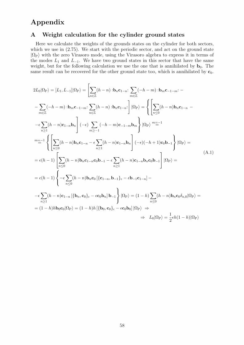
Appendix

A Weight calculation for the cylinder ground states

Here we calculate the weights of the grounds states on the cylinder for both sectors,which we use in (2.75). We start with the periodic sector, and act on the ground state|ΩP〉 with the zero Virasoro mode, using the Virasoro algebra to express it in terms ofthe modes L1 and L−1. We have two ground states in this sector that have the sameweight, but for the following calculation we use the one that is annihilated by b0. Thesame result can be recovered for the other ground state too, which is annihilated by c0.

2L0|ΩP〉 = [L1, L−1]|ΩP〉 =

[∑n∈Z

(h− n) :bnc1−n:∑m∈Z

(−h−m) :bmc−1−m: −

−∑m∈Z

(−h−m) :bmc−1−m:∑n∈Z

(h− n) :bnc1−n:

]|ΩP〉 =

∑n≤0

(h− n)bnc1−n −

−ε∑n≥1

(h− n)c1−nbn

(−ε)∑m≥−1

(−h−m)c−1−mbm

|ΩP〉m=−1

=

m=−1=

∑n≤0

(h− n)bnc1−n − ε∑n≥1

(h− n)c1−nbn

(−ε)(−h+ 1)c0b−1

|ΩP〉 =

= ε(h− 1)

∑n≤0

(h− n)bnc1−nc0b−1 − ε∑n≥1

(h− n)c1−nbnc0b−1

|ΩP〉 =

= ε(h− 1)

−ε∑n≤0

(h− n)bnc0 [c1−n,b−1ε − εb−1c1−n]−

−ε∑n≥1

(h− n)c1−n [bn, c0ε − εc0bn]b−1

|ΩP〉 = (1− h)∑n≤0

(h− n)bnc0δn,0|ΩP〉 =

= (1− h)hb0c0|ΩP〉 = (1− h)h [b0, c0ε − εc0b0] |ΩP〉 ⇒

⇒ L0|ΩP〉 =1

2εh(1− h)|ΩP〉

(A.1)

58

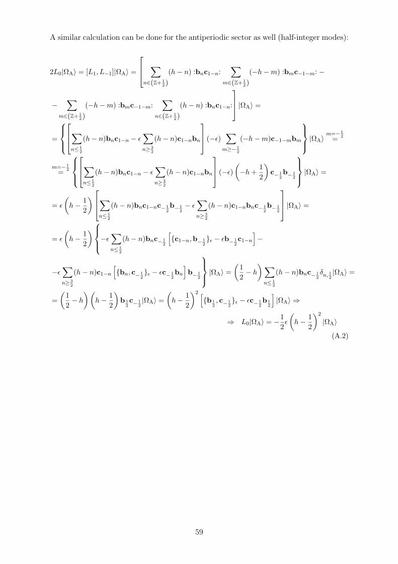
A similar calculation can be done for the antiperiodic sector as well (half-integer modes):

2L0|ΩA〉 = [L1, L−1]|ΩA〉 =

∑n∈(Z+ 1

2)

(h− n) :bnc1−n:∑

m∈(Z+ 12)

(−h−m) :bmc−1−m: −

−∑

m∈(Z+ 12)

(−h−m) :bmc−1−m:∑

n∈(Z+ 12)

(h− n) :bnc1−n:

|ΩA〉 =

=

∑n≤ 1

2

(h− n)bnc1−n − ε∑n≥ 3

2

(h− n)c1−nbn

(−ε)∑m≥− 1

2

(−h−m)c−1−mbm

|ΩA〉m=− 1

2=

m=− 12=

∑n≤ 1

2

(h− n)bnc1−n − ε∑n≥ 3

2

(h− n)c1−nbn

(−ε)(−h+

1

2

)c− 1

2b− 1

2

|ΩA〉 =

= ε

(h− 1

2

)∑n≤ 1

2

(h− n)bnc1−nc− 12b− 1

2− ε

∑n≥ 3

2

(h− n)c1−nbnc− 12b− 1

2

|ΩA〉 =

= ε

(h− 1

2

)−ε∑n≤ 1

2

(h− n)bnc− 12

[c1−n,b− 1

2ε − εb− 1

2c1−n

]−

−ε∑n≥ 3

2

(h− n)c1−n

[bn, c− 1

2ε − εc− 1

2bn

]b− 1

2

|ΩA〉 =

(1

2− h)∑n≤ 1

2

(h− n)bnc− 12δn, 1

2|ΩA〉 =

=

(1

2− h)(

h− 1

2

)b 1

2c− 1

2|ΩA〉 =

(h− 1

2

)2 [b 1

2, c− 1

2ε − εc− 1

2b 1

2

]|ΩA〉 ⇒

⇒ L0|ΩA〉 = −1

2ε

(h− 1

2

)2

|ΩA〉

(A.2)

59

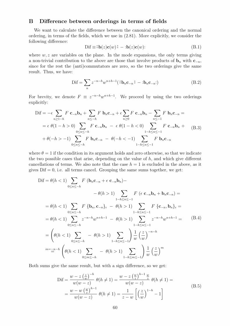
B Difference between orderings in terms of fields

We want to calculate the difference between the canonical ordering and the normalordering, in terms of the fields, which we use in (2.81). More explicitly, we consider thefollowing difference:

Dif ≡ aab(z)c(w)aa − :b(z)c(w): (B.1)

where w, z are variables on the plane. In the mode expansions, the only terms givinga non-trivial contribution to the above are those that involve products of bn with c−n,since for the rest the (anti)commutators are zero, so the two orderings give the sameresult. Thus, we have:

Dif =∑n

z−n−hwn+h−1(aabnc−n aa − :bnc−n:) (B.2)

For brevity, we denote F ≡ z−n−hwn+h−1. We proceed by using the two orderingsexplicitly:

Dif = −ε∑n≥1−h

F c−nbn +∑n≤−h

F bnc−n + ε∑n≥0

F c−nbn −∑n≤−1

F bnc−n =

= ε θ(1− h > 0)∑

0≤n≤−h

F c−nbn − ε θ(1− h < 0)∑

1−h≤n≤−1

F c−nbn +

+ θ(−h > −1)∑

0≤n≤−h

F bnc−n − θ(−h < −1)∑

1−h≤n≤−1

F bnc−n

(B.3)

where θ = 1 if the condition in its argument holds and zero otherwise, so that we indicatethe two possible cases that arise, depending on the value of h, and which give differentcancellations of terms. We also note that the case h = 1 is excluded in the above, as itgives Dif = 0, i.e. all terms cancel. Grouping the same sums together, we get:

Dif = θ(h < 1)∑

0≤n≤−h

F (bnc−n + ε c−nbn)−

− θ(h > 1)∑

1−h≤n≤−1

F (ε c−nbn + bnc−n) =

= θ(h < 1)∑

0≤n≤−h

F bn, c−nε − θ(h > 1)∑

1−h≤n≤−1

F c−n,bnε =

= θ(h < 1)∑

0≤n≤−h

z−n−hwn+h−1 − θ(h > 1)∑

1−h≤n≤−1

z−n−hwn+h−1 =

=

(θ(h < 1)

∑0≤n≤−h

− θ(h > 1)∑

1−h≤n≤−1

)1

w

( zw

)−n−hm=−n−h

=

(θ(h < 1)

∑0≤m≤−h

− θ(h > 1)∑

1−h≤m≤−1

)1

w

( zw

)m

(B.4)

Both sums give the same result, but with a sign difference, so we get:

Dif =w − z

(zw

)−hw(w − z)

θ(h 6= 1) =w − z

(wz

)h−1 wz

w(w − z)θ(h 6= 1) =

=w − w

(wz

)h−1

w(w − z)θ(h 6= 1) =

1

z − w

[( zw

)1−h− 1

] (B.5)

60

from which it is manifest that the case h = 1 gives zero. Thus, we conclude that thedifference between the two orderings in not a primary field. We also notice that despiteDif 6= 0 for h = 0, we have A = 0, according to (2.75). This means that the two orderingsagree for L0, despite Dif being non-zero. The resolution of this comes from the fact thatin this case, the difference between the two orderings is killed by the n = 0 term of L0,since there is an overall factor of (−n) multiplying the modes.

C Jacobi theta functions

Here we list the two-variable Jacobi theta functions:

θ1(τ, z) ≡ −i∑

n∈(Z+ 12)

(−1)n−12 ynqn

2/2 =

= −iq1/8(y1/2 − y−1/2

) ∞∏n=1

(1− qn) (1− yqn)(1− y−1qn

)θ2(τ, z) ≡

∑n∈(Z+ 1

2)

ynqn2/2 = q1/8

(y1/2 + y−1/2

) ∞∏n=1

(1− qn) (1 + yqn)(1 + y−1qn

)θ3(τ, z) ≡

∑n∈Z

ynqn2/2 =

∞∏n=1

(1− qn)(

1 + yqn−1/2)(

1 + y−1qn−1/2)

θ4(τ, z) ≡=∑n∈Z

(−1)nynqn2/2 =

∞∏n=1

(1− qn)(

1− yqn−1/2)(

1− y−1qn−1/2)

(C.1)

These can be packed together into a four-component vector-valued Jacobi form of weight1/2 and index 1/2, while the usual theta functions are retrieved for z = 0. A Jacobi formof weight k and index t is defined as a function that has the following transformationproperties under under the Jacobi group SL(2,Z) n Z2 34:

φ

(aτ + b

cτ + d,

z

cτ + d

)= (cτ + d)k exp

(2πit

cz2

cτ + d

)φ(τ, z) ,

(a bc d

)∈ SL(2,Z)

φ(τ, z + λτ + µ) = exp[−2πit(λ2τ + 2λz)

]φ(τ, z) , λ, µ ∈ Z

(C.2)

Moreover, we also define the Dedekind eta function:

η(τ) ≡ q1/24

∞∏n=1

(1− qn) (C.3)

which is a modular form of weight 1/2. A modular form transforms as a Jacobi form ofindex 0:

φ

(aτ + b

cτ + d

)= (cτ + d)k φ(τ) ,

(a bc d

)∈ SL(2,Z) (C.4)

The Dedekind eta function is related to the theta functions through the notable identity:

η(τ)3 =1

2θ2(τ, 0)θ3(τ, 0)θ4(τ, 0) (C.5)

34n stands for semidirect product, which means that(SL(2,Z) n Z2

)/Z2 ∼= SL(2,Z) but(

SL(2,Z) n Z2)/SL(2,Z) is not isomorphic to Z2

61

References

[1] D. Friedan, E. Martinec, S. Shenker, Conformal invariance, supersymmetry andstring theory, Nucl. Phys. B271 (1986) 93-165

[2] P. Ginsparg, Applied conformal field theory, Les Houches, Session XLIX (1988), ed.by E. Brezin and J. Zinn Justin (1989), [arXiv:hep-th/9108028]

[3] R. Blumenhagen, D. Lust, S. Theisen, Basic concepts of string theory, Springer BerlinHeidelberg, Berlin, Heidelberg 2013 Springer Science and Business Media B.V.

[4] R. Blumenhagen, E. Plauschinn, Introduction to conformal field theory, with appli-cations to string theory, Berlin, Heidelberg, Springer-Verlag Berlin Heidelberg, 2009

[5] P. Di Francesco, P. Mathieu, D. Senechal, Conformal field theory, New York, Springercop. 1997

[6] D. Tong, Lectures on string theory, [arXiv:0908.0333]

[7] S. Guruswamy, A. W.W. Ludwig, Relating c < 0 and c > 0 Conformal FieldTheories, Nuclear Physics, Section B, 1998, Vol.519(3), pp.661-681, [arXiv:hep-th/9612172v1]

[8] H. G. Kausch, Curiosities at c = −2, 1995, [arXiv:hep-th/9510149v1]

[9] H. G. Kausch, Symplectic fermions, Nuclear Physics, Section B, 2000, Vol.583(3),pp.513-541, [arXiv:hep-th/0003029v2]

[10] T. Eguchi, H. Ooguri, Y. Tachikawa, Notes on the K3 surface and the Mathieugroup M24, Exper. Math. 20 , 91 (2011), [arXiv:1004.0956]

[11] M. C. N. Cheng, The spectra of supersymmetric states in string theory, PhD thesis,University of Amsterdam (2008)

[12] M. C. N. Cheng, J. F. R. Duncan, The Largest Mathieu Group and (Mock) Auto-morphic Forms, 2012, [arXiv:1201.4140]

[13] M. C. N. Cheng, Lecture notes on automorphic forms and physics, Heidelberg (2011)

[14] M. C. N. Cheng, X. Dong, J. F. R. Duncan, S. Harrison, S. Kachru, T. Wrase, Mockmodular mathieu moonshine modules, Research in the Mathematical Sciences, 2015,Vol.2(1), pp.1-89, [arXiv:1406.5502v2]

[15] M. B. Green, J. H. Schwarz, E. Witten, Superstring theory, Volumes 1 and 2,Cambridge, Cambridge University Press 1987

[16] J. Polchinski, String theory, Vol 1: An introduction of the bosonic string and Vol2:Superstring theory and beyond, Cambridge, Cambridge University Press cop. 1998

[17] F. Malikov, V. Schechtman, A. Vaintrob, Chiral de Rham complex, Comm. Math.Phys. 204 (1999) 439, [arXiv:math.AG/9803041v7]

[18] V. Kac, Vertex algebras for beginners, University Lecture Series, 10, AmericanMathematical Society, Providence, RI, 1997

62

[19] K. Wendland, Moduli spaces of unitary conformal field theories, PhD thesis, Uni-versity of Bonn (2000)

[20] K. Wendland, Snapshots of conformal field theory, 2014, [arXiv:1404.3108v1]

[21] L. A. Borisov, A. Libgober, Elliptic genera of toric varieties and applications tomirror symmetry, Invent. Math. 140 (2000) 453, [arXiv:math/9904126v1]

[22] L. A. Borisov, Vertex algebras and mirror symmetry, Comm. in Math. Phys., 2001,Vol.215(3), pp.517-557, [arXiv:math/9809094v2]

[23] E. Witten, Mirror manifolds and topological field theory, in Essays on Mirror Mani-folds, pp. 120-158, ed. S. T. Yau, International Press, Hong Kong, 1992, [arXiv:hep-th/9112056v1]

[24] E. Witten, Elliptic genera and quantum field theory, Comm. in Math. Phys., 1987,Vol.109(4), pp.525-536

[25] E. Witten, On the Landau-Ginzburg description of N = 2 minimal models, In-ternational Journal Of Modern Physics A, 1994 Oct 30, Vol.9(27), pp.4783-4800,[arXiv:hep-th/9304026]

[26] T. Kawai, Y. Yamada, S. K. Yang, Elliptic genera and N = 2 superconformalfield theory, Nuclear Physics, Section B, 14 February 1994, Vol.414(1-2), pp.191-212,[arXiv:hep-th/9306096v2]

[27] R. Dijkgraaf, G. Moore, E. Verlinde, H. Verlinde, Elliptic genera of symmetricproducts and second quantized strings, Comm. in Math. Phys., 1997, Vol.185(1),pp.197-209, [arXiv:hep-th/9608096v2]

[28] A. Kapustin, Chiral de Rham complex and the half-twisted sigma-model, 2005,[arXiv:hep-th/0504074v1]

[29] K. Hori, S. Katz, A. Klemm, R. Pandharipande, R. Thomas, C. Vafa, R. Vakil,E. Zaslow, Mirror Symmetry, American Mathematical Society, Clay MathematicsInstitute, 2003

[30] M. Nakahara, Geometry, topology, and physics, Boca Raton, Taylor and FrancisGroup, 2nd ed. (2003)

[31] V. Bouchard, Lectures on complex geometry, Calabi-Yau manifolds and toric geom-etry, 2007, [arXiv:hep-th/0702063v1]

[32] A. M. Semikhatov, I. Y. Tipunin, All singular vectors of the N = 2 superconformalalgebra via the algebraic continuation approach, 1998, [arXiv:hep-th/9604176]

[33] T. Eguchi, H. Ooguri, A. Taormina, S-K Yang, Superconformal algebras and stringcompactification on manifolds with SU(N) holonomy, Nuclear Physics, Section B,1989, Vol.315(1), pp.193-221

[34] T. Eguchi, S-K Yang, N = 2 superconformal models as topological field theories,Modern Physics Letters A, 1990, Vol.05(21), pp.1693-1701

63