Bayesian Methods - courses.cs.washington.edu · ©2017 Kevin Jamieson 1 Bayesian Methods Machine...
35
©2017 Kevin Jamieson 1 Bayesian Methods Machine Learning – CSE546 Kevin Jamieson University of Washington September 28, 2017
Transcript of Bayesian Methods - courses.cs.washington.edu · ©2017 Kevin Jamieson 1 Bayesian Methods Machine...
©2017 Kevin Jamieson 1
Bayesian Methods
Machine Learning – CSE546 Kevin Jamieson University of Washington
September 28, 2017
2©2017 Kevin Jamieson
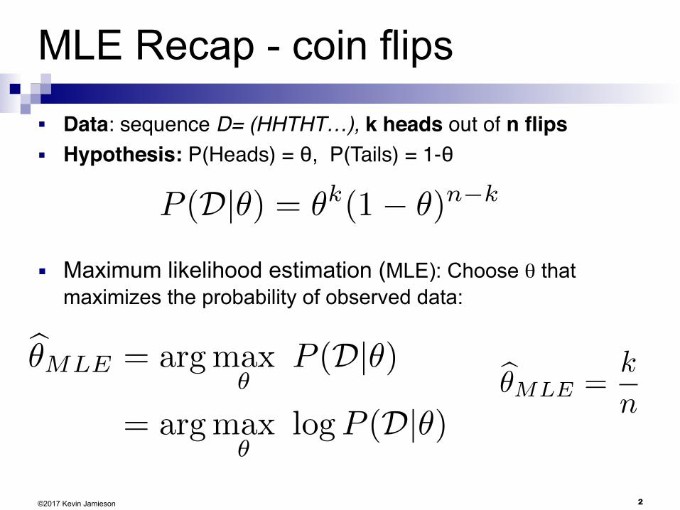
MLE Recap - coin flips
■ Data: sequence D= (HHTHT…), k heads out of n flips■ Hypothesis: P(Heads) = θ, P(Tails) = 1-θ
■ Maximum likelihood estimation (MLE): Choose θ that maximizes the probability of observed data:
P (D|✓) = ✓k(1� ✓)n�k
b✓MLE = argmax
✓P (D|✓)
= argmax
✓logP (D|✓)
b✓MLE =k
n
3©2017 Kevin Jamieson
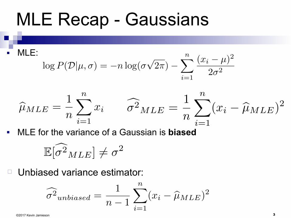
MLE Recap - Gaussians
■ MLE:
■ MLE for the variance of a Gaussian is biased
Unbiased variance estimator:
bµMLE =1
n
nX
i=1
xic�
2MLE =
1
n
nX
i=1
(xi � bµMLE)2
E[c�2MLE ] 6= �2
c�
2unbiased =
1
n� 1
nX
i=1
(xi � bµMLE)2
logP (D|µ,�) = �n log(�
p2⇡)�
nX
i=1
(xi � µ)
2
2�
2
MLE Recap
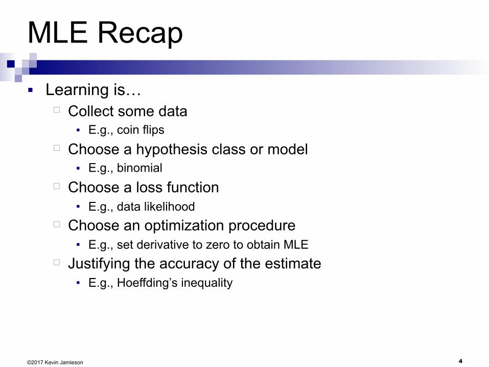
■ Learning is… Collect some data ■ E.g., coin flips
Choose a hypothesis class or model ■ E.g., binomial
Choose a loss function ■ E.g., data likelihood
Choose an optimization procedure ■ E.g., set derivative to zero to obtain MLE
Justifying the accuracy of the estimate ■ E.g., Hoeffding’s inequality
4©2017 Kevin Jamieson
5©2017 Kevin Jamieson
What about prior
■ Billionaire: Wait, I know that the coin is “close” to 50-50. What can you do for me now?
■ You say: I can learn it the Bayesian way…
6©2017 Kevin Jamieson
Bayesian vs Frequentist
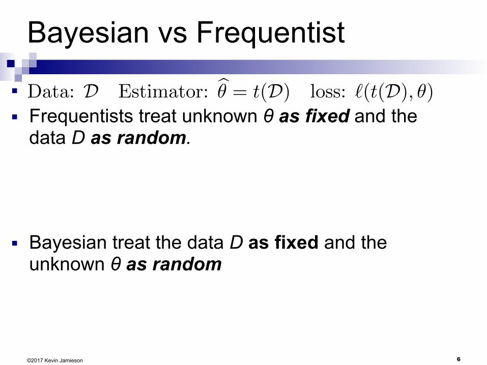
■ ■ Frequentists treat unknown θ as fixed and the
data D as random.
■ Bayesian treat the data D as fixed and the unknown θ as random
Data: D Estimator:
b✓ = t(D) loss: `(t(D), ✓)
7©2017 Kevin Jamieson
Bayesian Learning
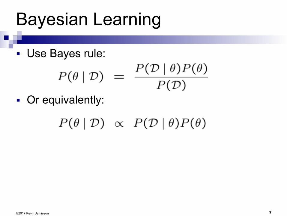
■ Use Bayes rule:
■ Or equivalently:
8©2017 Kevin Jamieson
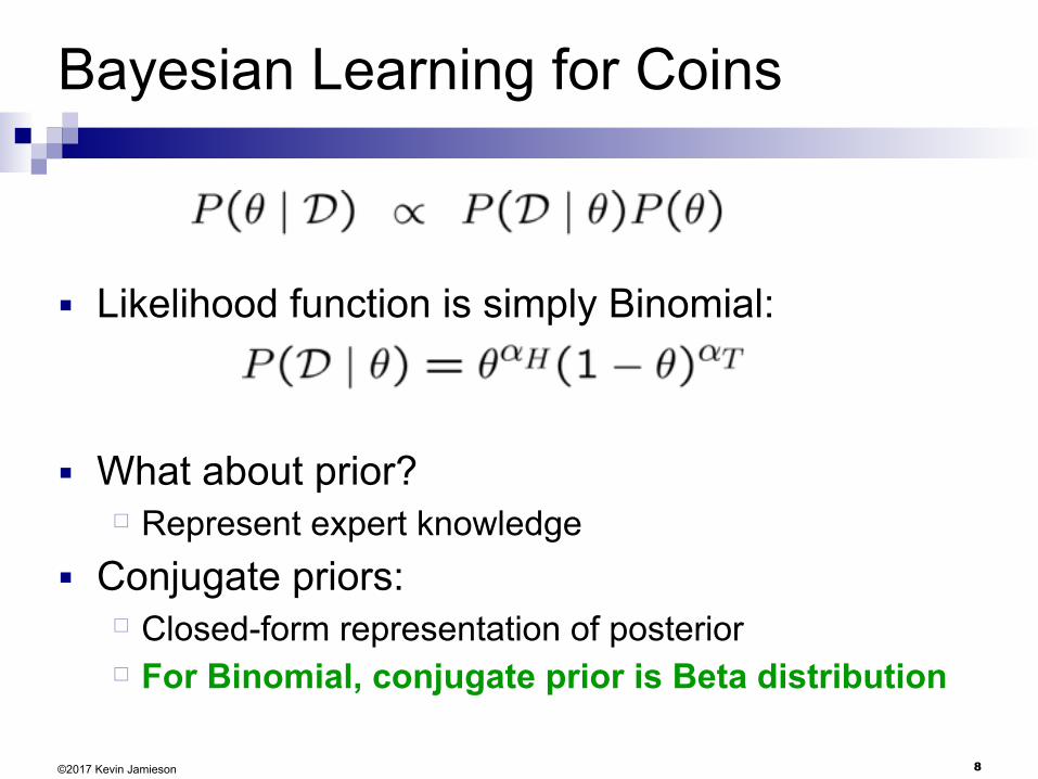
Bayesian Learning for Coins
■ Likelihood function is simply Binomial:
■ What about prior? Represent expert knowledge
■ Conjugate priors: Closed-form representation of posterior For Binomial, conjugate prior is Beta distribution
9©2017 Kevin Jamieson
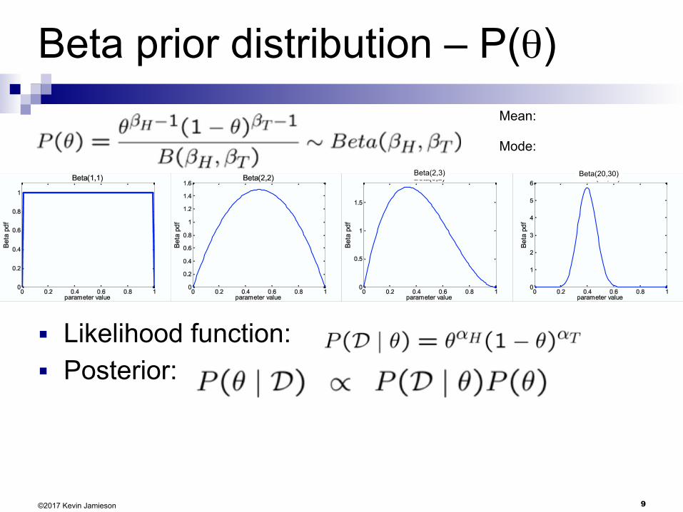
Beta prior distribution – P(θ)
■ Likelihood function: ■ Posterior:
Mean:
Mode:
Beta(2,3) Beta(20,30)
10©2017 Kevin Jamieson
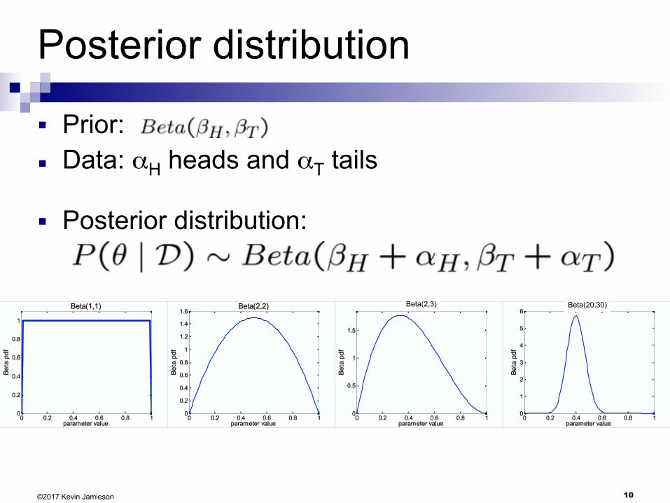
Posterior distribution
■ Prior: ■ Data: αH heads and αT tails
■ Posterior distribution:
Beta(2,3) Beta(20,30)
11©2017 Kevin Jamieson
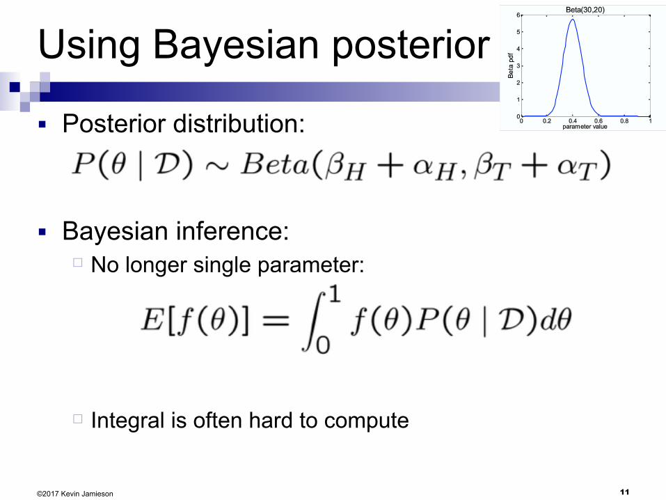
Using Bayesian posterior
■ Posterior distribution:
■ Bayesian inference: No longer single parameter:
Integral is often hard to compute
12©2017 Kevin Jamieson
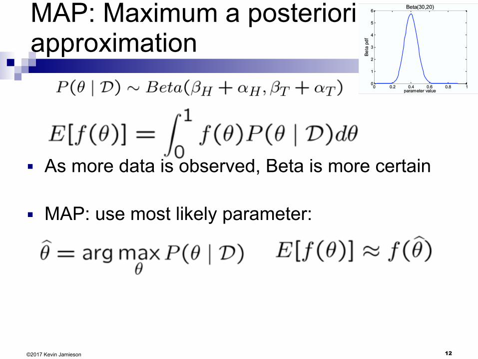
MAP: Maximum a posteriori approximation
■ As more data is observed, Beta is more certain
■ MAP: use most likely parameter:
13©2017 Kevin Jamieson
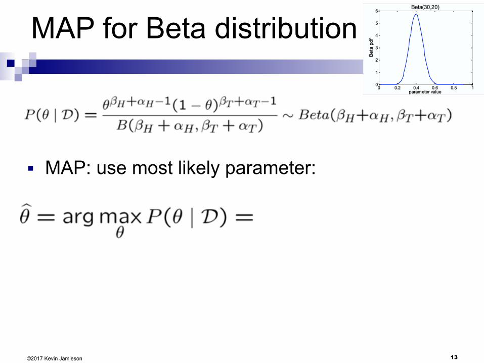
MAP for Beta distribution
■ MAP: use most likely parameter:
14©2017 Kevin Jamieson
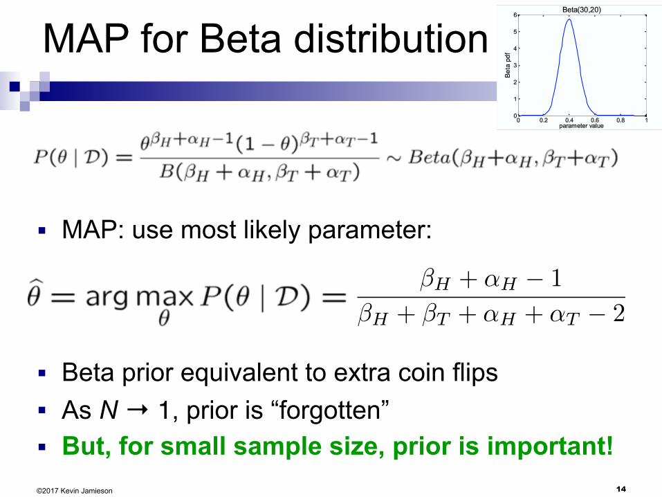
MAP for Beta distribution
■ MAP: use most likely parameter:
■ Beta prior equivalent to extra coin flips ■ As N → 1, prior is “forgotten” ■ But, for small sample size, prior is important!
�H + ↵H � 1
�H + �T + ↵H + ↵T � 2
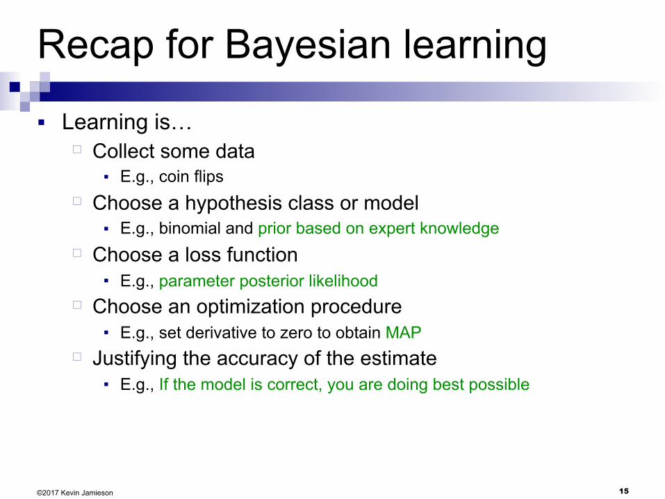
Recap for Bayesian learning
■ Learning is… Collect some data ■ E.g., coin flips
Choose a hypothesis class or model ■ E.g., binomial and prior based on expert knowledge
Choose a loss function ■ E.g., parameter posterior likelihood
Choose an optimization procedure ■ E.g., set derivative to zero to obtain MAP
Justifying the accuracy of the estimate ■ E.g., If the model is correct, you are doing best possible
15©2017 Kevin Jamieson
Recap for Bayesian learning
16©2017 Kevin Jamieson
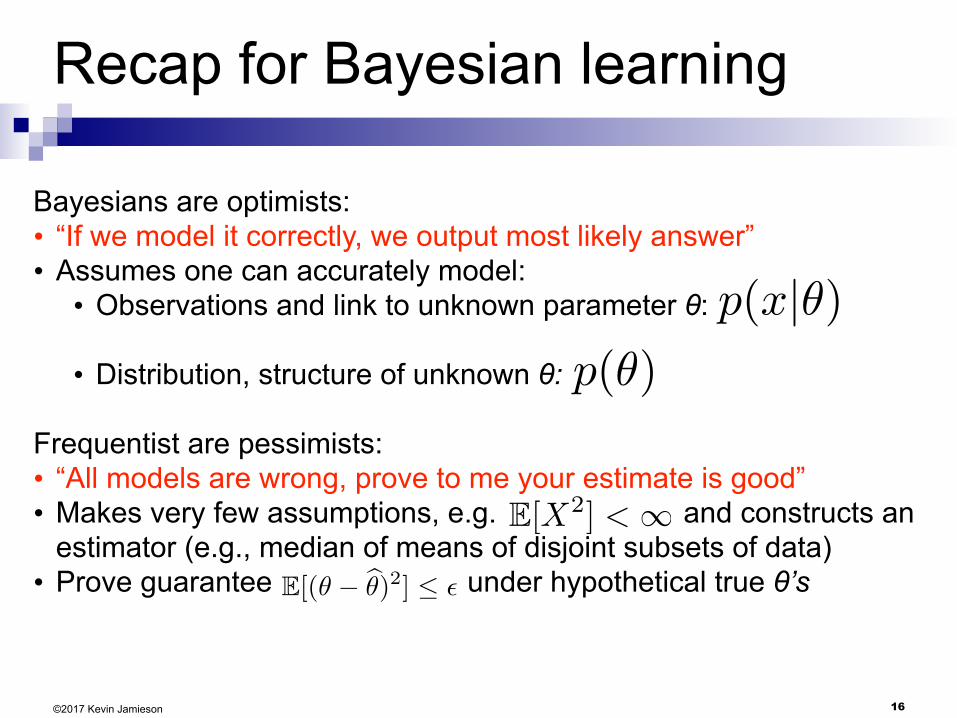
Bayesians are optimists: • “If we model it correctly, we output most likely answer” • Assumes one can accurately model:
• Observations and link to unknown parameter θ:
• Distribution, structure of unknown θ:
Frequentist are pessimists: • “All models are wrong, prove to me your estimate is good” • Makes very few assumptions, e.g. and constructs an
estimator (e.g., median of means of disjoint subsets of data) • Prove guarantee under hypothetical true θ’s
p(x|✓)p(✓)
E[X2] < 1
E[(✓ � b✓)2] ✏

©2017 Kevin Jamieson 17
Linear Regression
Machine Learning – CSE546 Kevin Jamieson University of Washington
Oct 3, 2017
18
The regression problem
©2017 Kevin Jamieson
# square feet
Sal
e P
rice
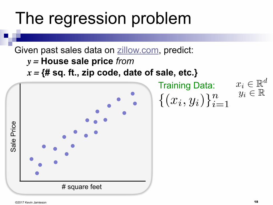
Given past sales data on zillow.com, predict: y = House sale price from x = {# sq. ft., zip code, date of sale, etc.}
Training Data:
{(xi, yi)}ni=1
xi 2 Rd
yi 2 R
19
The regression problem
©2017 Kevin Jamieson
# square feet
Sal
e P
rice
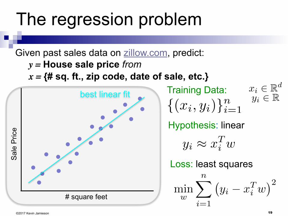
Given past sales data on zillow.com, predict: y = House sale price from x = {# sq. ft., zip code, date of sale, etc.}
Training Data:
{(xi, yi)}ni=1
xi 2 Rd
yi 2 R
Hypothesis: linear
Loss: least squares
yi ⇡ x
Ti w
minw
nX
i=1
�yi � x
Ti w
�2
best linear fit
20©2017 Kevin Jamieson
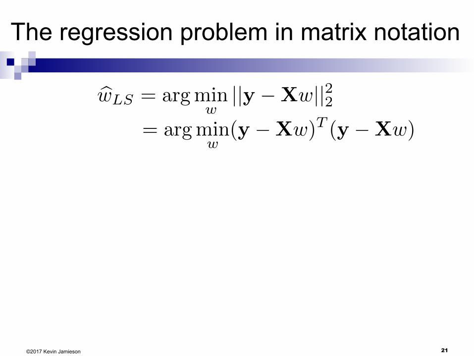
The regression problem in matrix notation
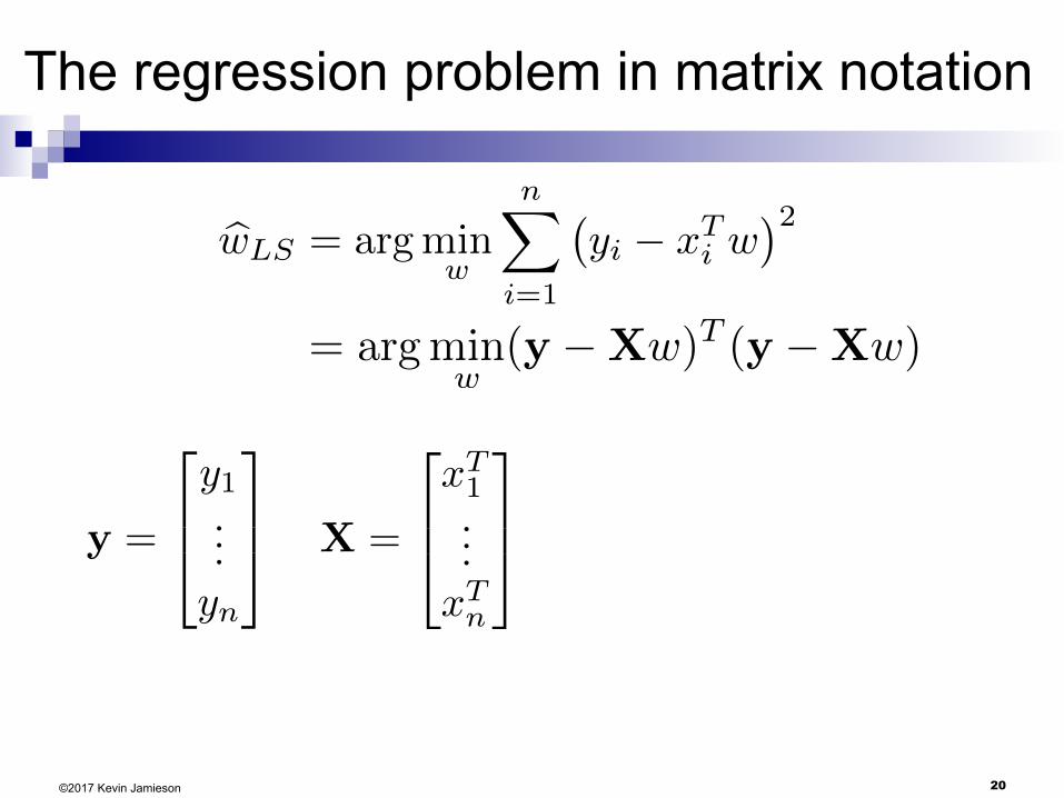
y =
2
64y1...yn
3
75 X =
2
64x
T1...x
Tn
3
75
= argminw
(y �Xw)T (y �Xw)
bwLS = argminw
nX
i=1
�yi � x
Ti w
�2
21©2017 Kevin Jamieson
The regression problem in matrix notation
= argminw
(y �Xw)T (y �Xw)
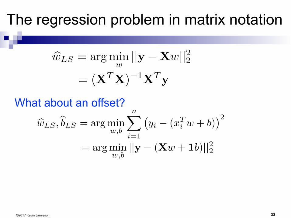
bwLS = argminw
||y �Xw||22
22©2017 Kevin Jamieson
The regression problem in matrix notation
= (XTX)�1XTy
bwLS = argminw
||y �Xw||22
What about an offset?
bwLS ,bbLS = argmin
w,b
nX
i=1
�yi � (xT
i w + b)�2
= argminw,b
||y � (Xw + 1b)||22
23©2017 Kevin Jamieson
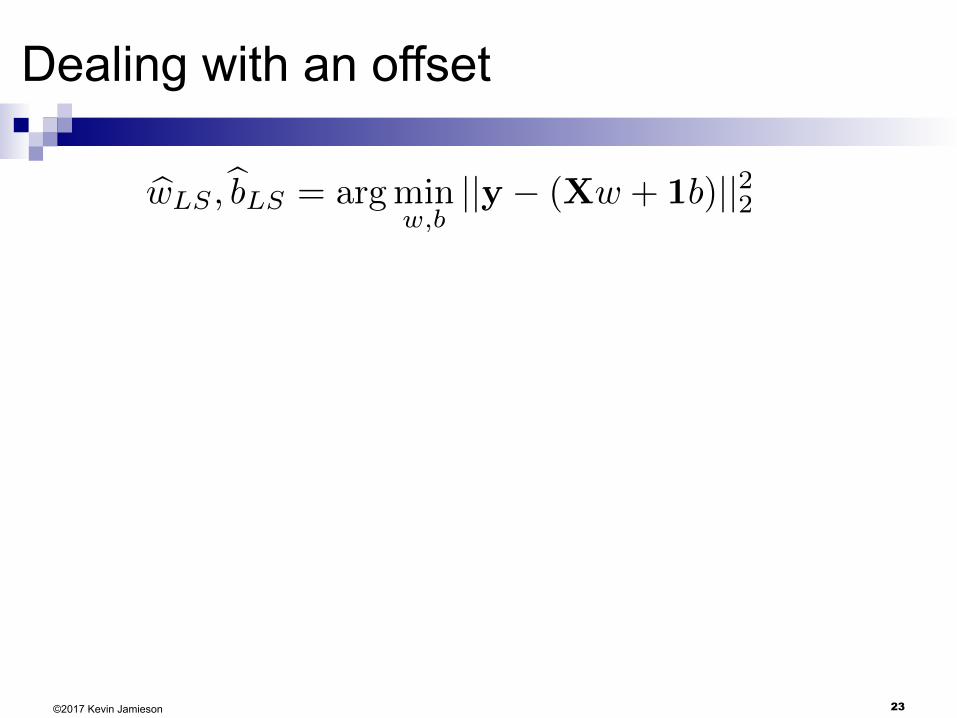
Dealing with an offset
bwLS ,bbLS = argminw,b
||y � (Xw + 1b)||22
24©2017 Kevin Jamieson
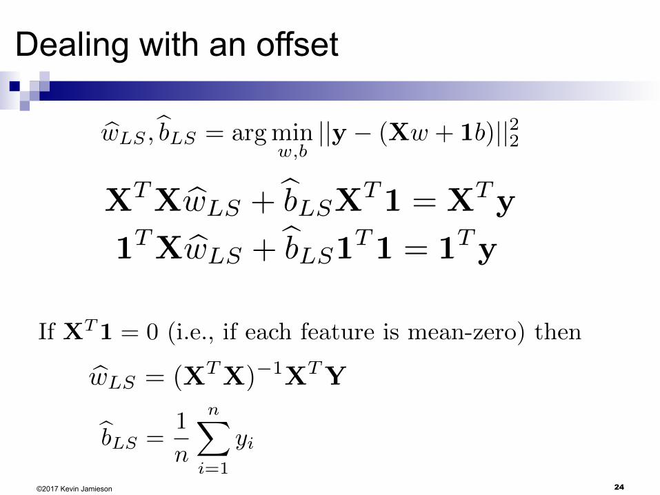
Dealing with an offset
If XT1 = 0 (i.e., if each feature is mean-zero) then
bwLS = (XTX)�1XTY
bbLS =1
n
nX
i=1
yi
XTX bwLS +bbLSXT1 = XTy
1TX bwLS +bbLS1T1 = 1Ty
bwLS ,bbLS = argminw,b
||y � (Xw + 1b)||22
25©2017 Kevin Jamieson
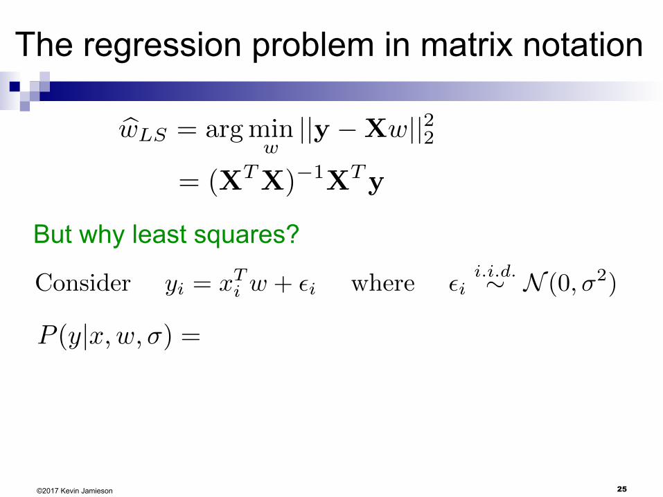
The regression problem in matrix notation
= (XTX)�1XTy
bwLS = argminw
||y �Xw||22
But why least squares?
Consider yi = x
Ti w + ✏i where ✏i
i.i.d.⇠ N (0,�
2)
P (y|x,w,�) =
26
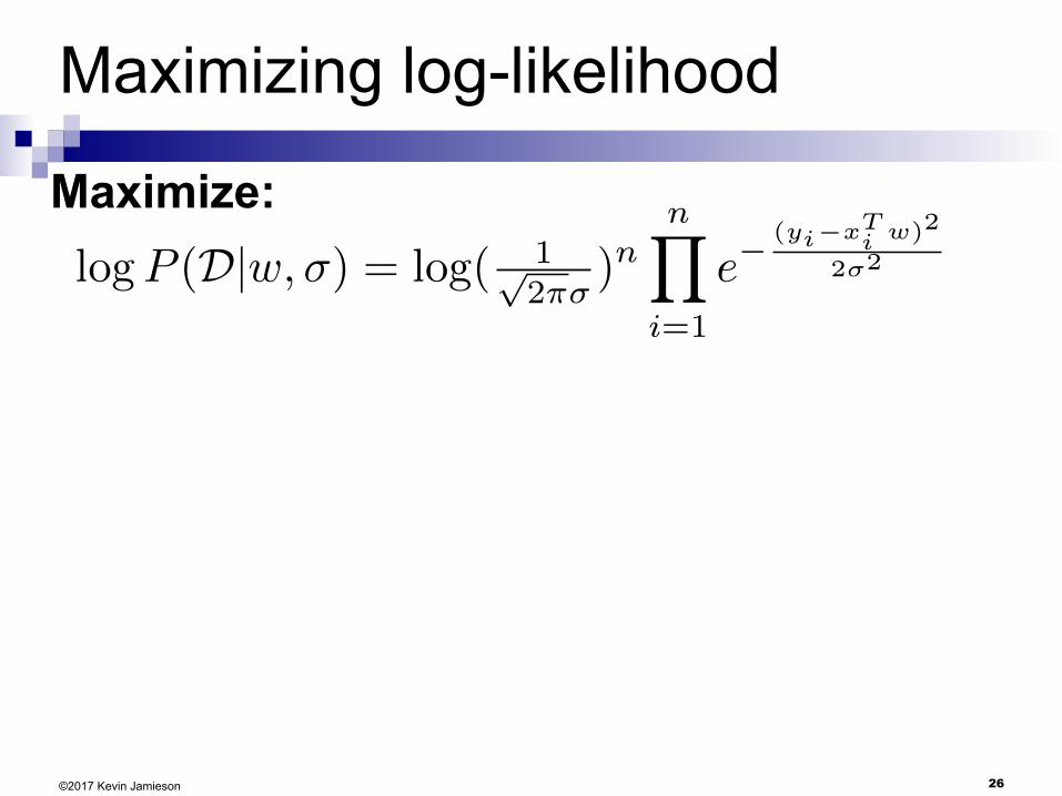
Maximizing log-likelihood
Maximize:
©2017 Kevin Jamieson
logP (D|w,�) = log(
1p2⇡�
)
nnY
i=1
e�(y
i
�x
T
i
w)2
2�2
27
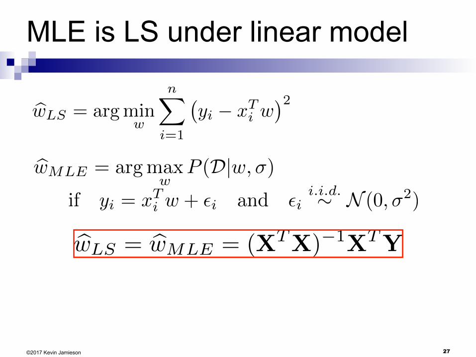
MLE is LS under linear model
©2017 Kevin Jamieson
bwLS = argminw
nX
i=1
�yi � x
Ti w
�2
if yi = x
Ti w + ✏i and ✏i
i.i.d.⇠ N (0,�2)
bwMLE = argmax
wP (D|w,�)
bwLS = bwMLE = (XTX)�1XTY

28
The regression problem
©2017 Kevin Jamieson
# square feet
Sal
e P
rice
Given past sales data on zillow.com, predict: y = House sale price from x = {# sq. ft., zip code, date of sale, etc.}
Training Data:
{(xi, yi)}ni=1
xi 2 Rd
yi 2 R
Hypothesis: linear
Loss: least squares
yi ⇡ x
Ti w
minw
nX
i=1
�yi � x
Ti w
�2
best linear fit
29
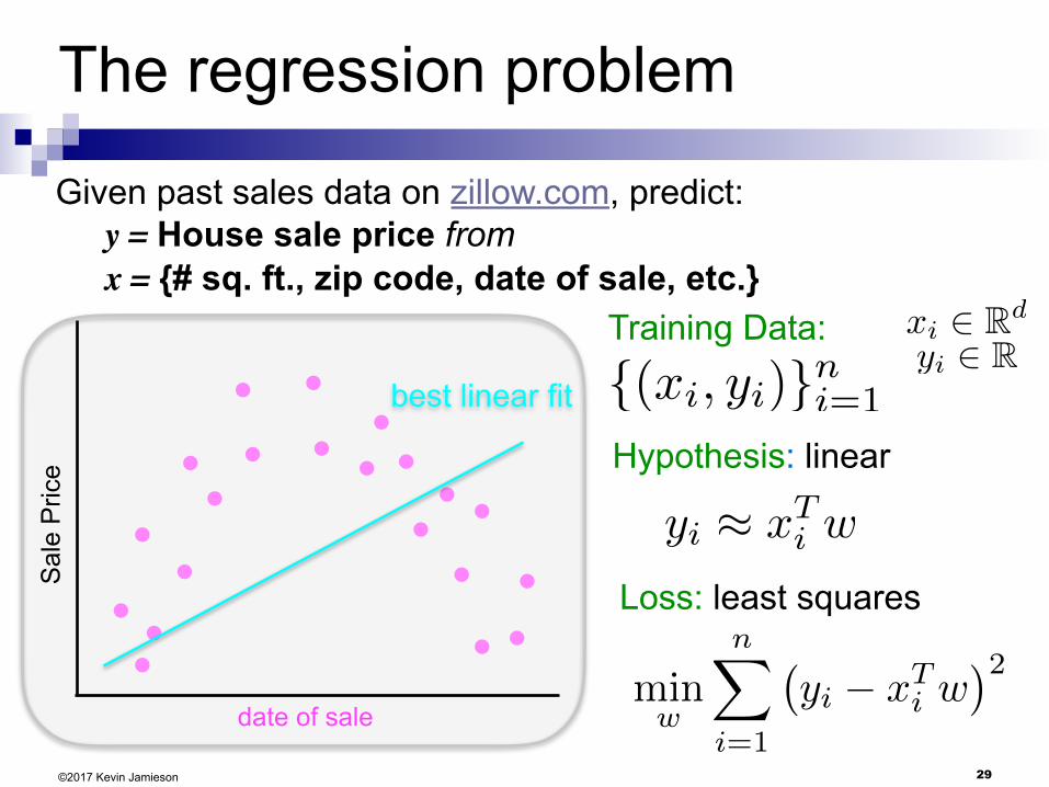
The regression problem
©2017 Kevin Jamieson
date of sale
Sal
e P
rice
Given past sales data on zillow.com, predict: y = House sale price from x = {# sq. ft., zip code, date of sale, etc.}
Training Data:
{(xi, yi)}ni=1
xi 2 Rd
yi 2 R
Hypothesis: linear
Loss: least squares
yi ⇡ x
Ti w
minw
nX
i=1
�yi � x
Ti w
�2
best linear fit
30
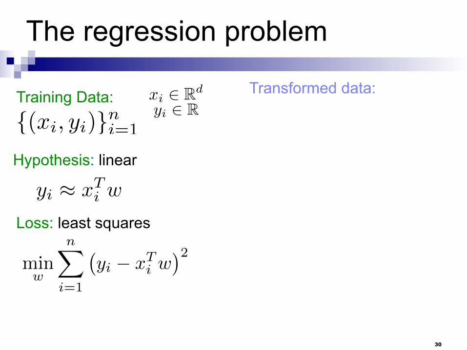
The regression problem
Training Data:
{(xi, yi)}ni=1
xi 2 Rd
yi 2 R
Hypothesis: linear
Loss: least squares
yi ⇡ x
Ti w
minw
nX
i=1
�yi � x
Ti w
�2
Transformed data:
31
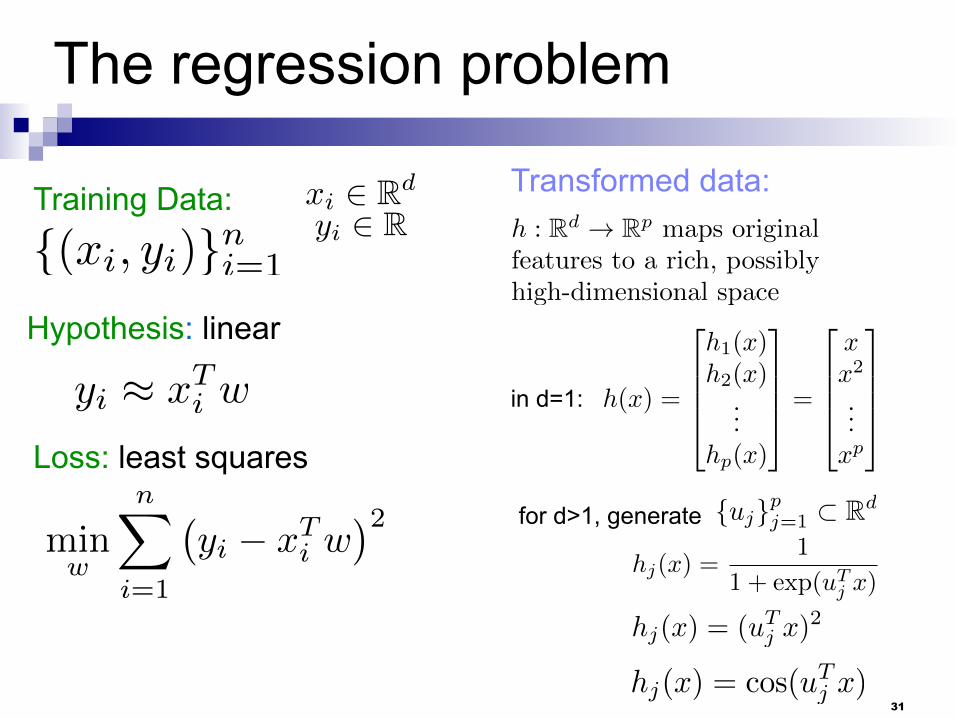
The regression problem
Training Data:
{(xi, yi)}ni=1
xi 2 Rd
yi 2 R
Hypothesis: linear
Loss: least squares
yi ⇡ x
Ti w
minw
nX
i=1
�yi � x
Ti w
�2
Transformed data:
in d=1:
h : Rd ! Rpmaps original
features to a rich, possibly
high-dimensional space
hj(x) =1
1 + exp(u
Tj x)
hj(x) = (uTj x)
2
for d>1, generate {uj}pj=1 ⇢ Rd
hj(x) = cos(u
Tj x)
h(x) =
2
6664
h1(x)h2(x)
...hp(x)
3
7775=
2
6664
x
x
2
...x
p
3
7775
32
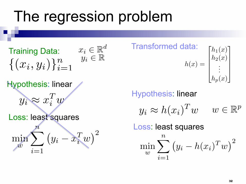
The regression problem
Training Data:
{(xi, yi)}ni=1
xi 2 Rd
yi 2 R
Hypothesis: linear
Loss: least squares
yi ⇡ x
Ti w
minw
nX
i=1
�yi � x
Ti w
�2
Transformed data:
h(x) =
2
6664
h1(x)h2(x)
...hp(x)
3
7775
Hypothesis: linear
Loss: least squares
yi ⇡ h(xi)Tw
w 2 Rp
minw
nX
i=1
�yi � h(xi)
Tw
�2
33
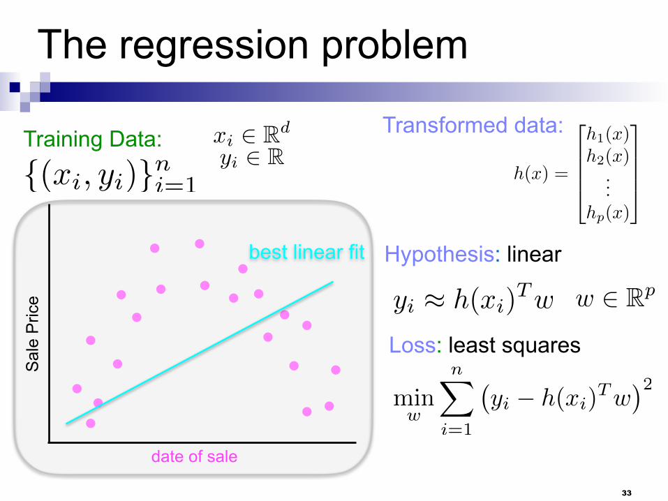
The regression problem
Training Data:
{(xi, yi)}ni=1
xi 2 Rd
yi 2 RTransformed data:
h(x) =
2
6664
h1(x)h2(x)
...hp(x)
3
7775
Hypothesis: linear
Loss: least squares
yi ⇡ h(xi)Tw
w 2 Rp
minw
nX
i=1
�yi � h(xi)
Tw
�2
date of sale
Sal
e P
rice
best linear fit
34
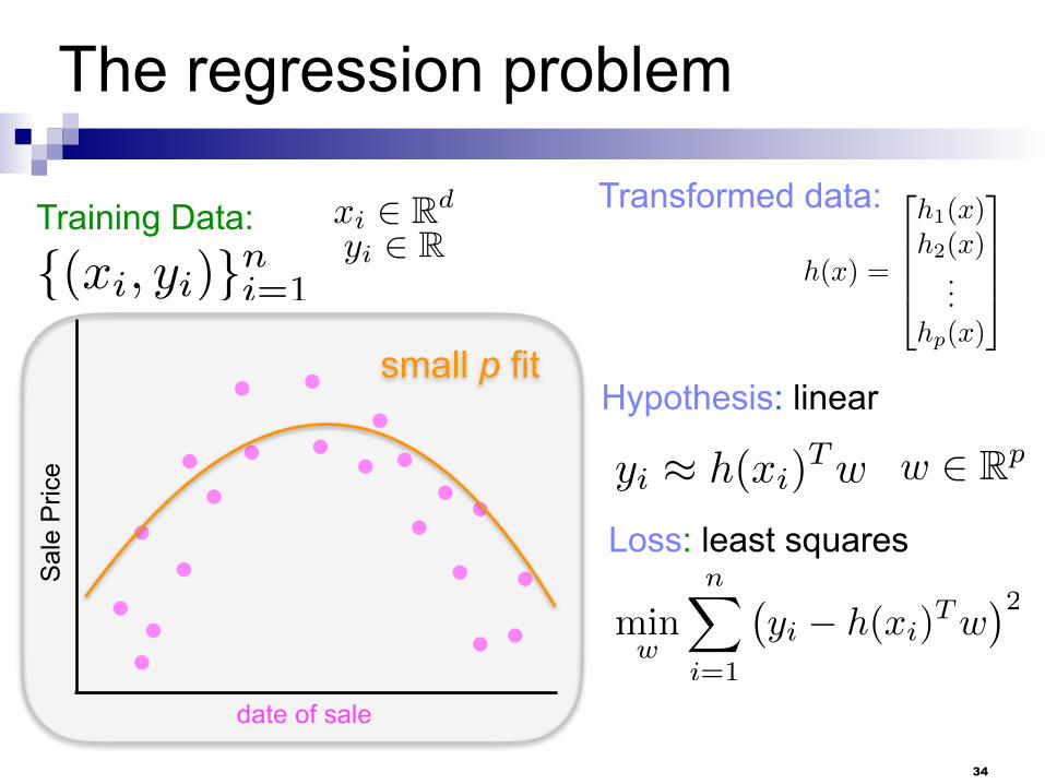
The regression problem
Training Data:
{(xi, yi)}ni=1
xi 2 Rd
yi 2 RTransformed data:
h(x) =
2
6664
h1(x)h2(x)
...hp(x)
3
7775
Hypothesis: linear
Loss: least squares
yi ⇡ h(xi)Tw
w 2 Rp
minw
nX
i=1
�yi � h(xi)
Tw
�2
date of sale
Sal
e P
rice
small p fit
35
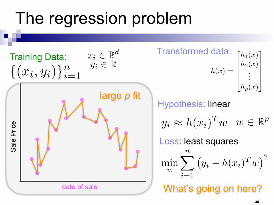
The regression problem
Training Data:
{(xi, yi)}ni=1
xi 2 Rd
yi 2 RTransformed data:
h(x) =
2
6664
h1(x)h2(x)
...hp(x)
3
7775
Hypothesis: linear
Loss: least squares
yi ⇡ h(xi)Tw
w 2 Rp
minw
nX
i=1
�yi � h(xi)
Tw
�2
date of sale
Sal
e P
rice
large p fit
What’s going on here?