Bayesian Decision and Bayesian Learning
30
Bayesian Decision and Bayesian Learning Ying Wu Electrical Engineering and Computer Science Northwestern University Evanston, IL 60208 http://www.eecs.northwestern.edu/~yingwu 1 / 30
Transcript of Bayesian Decision and Bayesian Learning
Bayesian Decision and Bayesian Learning
Ying Wu
Electrical Engineering and Computer ScienceNorthwestern University
Evanston, IL 60208
http://www.eecs.northwestern.edu/~yingwu
1 / 30
Bayes Rule
I p(x|ωi ) Likelihood
I p(ωi ) Prior
I p(ωi |x) Posterior
I Bayes Rule
p(ωi |x) =p(x|ωi )p(ωi )
p(x)=
p(x|ωi )p(ωi )∑i p(x|ωi )p(ωi )
I In other words
posterior ∝ likelihood× prior
2 / 30
Outline
Bayesian Decision Theory
Bayesian Classification
Maximum Likelihood Estimation and Learning
Bayesian Estimation and Learning
3 / 30
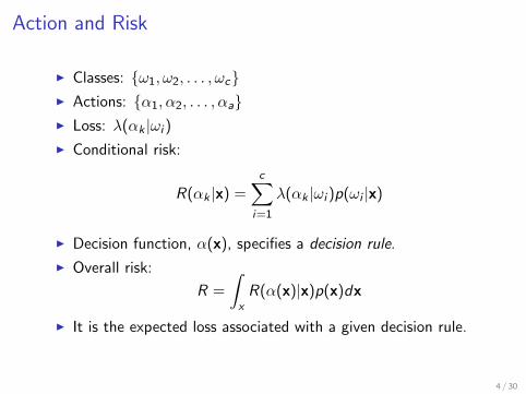
Action and Risk
I Classes: {ω1, ω2, . . . , ωc}I Actions: {α1, α2, . . . , αa}I Loss: λ(αk |ωi )
I Conditional risk:
R(αk |x) =c∑
i=1
λ(αk |ωi )p(ωi |x)
I Decision function, α(x), specifies a decision rule.
I Overall risk:
R =
∫x
R(α(x)|x)p(x)dx
I It is the expected loss associated with a given decision rule.
4 / 30
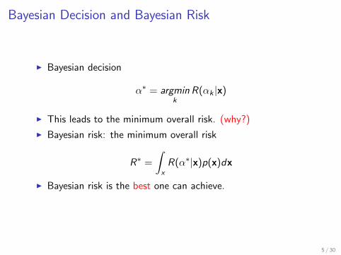
Bayesian Decision and Bayesian Risk
I Bayesian decision
α∗ = argmink
R(αk |x)
I This leads to the minimum overall risk. (why?)
I Bayesian risk: the minimum overall risk
R∗ =
∫x
R(α∗|x)p(x)dx
I Bayesian risk is the best one can achieve.
5 / 30
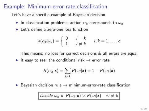
Example: Minimum-error-rate classification
Let’s have a specific example of Bayesian decision
I In classification problems, action αk corresponds to ωk
I Let’s define a zero-one loss function
λ(αk |ωi ) =
{0 i = k1 i 6= k
i , k = 1, . . . , c
This means: no loss for correct decisions & all errors are equal
I It easy to see: the conditional risk → error rate
R(αk |x) =∑i 6=k
P(ωi |x) = 1− P(ωk |x)
I Bayesian decision rule → minimum-error-rate classification
Decide ωk if P(ωk |x) > P(ωi |x) ∀i 6= k
6 / 30
Outline
Bayesian Decision Theory
Bayesian Classification
Maximum Likelihood Estimation and Learning
Bayesian Estimation and Learning
7 / 30
Classifier and Discriminant Functions
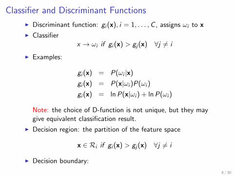
I Discriminant function: gi (x), i = 1, . . . ,C , assigns ωi to x
I Classifierx → ωi if gi (x) > gj(x) ∀j 6= i
I Examples:
gi (x) = P(ωi |x)
gi (x) = P(x|ωi )P(ωi )
gi (x) = ln P(x|ωi ) + ln P(ωi )
Note: the choice of D-function is not unique, but they maygive equivalent classification result.
I Decision region: the partition of the feature space
x ∈ Ri if gi (x) > gj(x) ∀j 6= i
I Decision boundary:
8 / 30
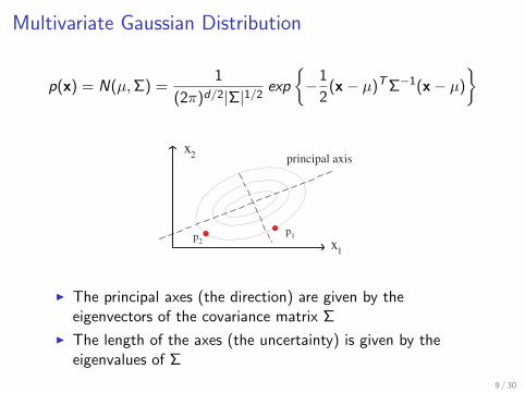
Multivariate Gaussian Distribution
p(x) = N(µ,Σ) =1
(2π)d/2|Σ|1/2exp
{−1
2(x− µ)TΣ−1(x− µ)
}
x 1
x 2 principal axis
p 1 p
2
I The principal axes (the direction) are given by theeigenvectors of the covariance matrix Σ
I The length of the axes (the uncertainty) is given by theeigenvalues of Σ
9 / 30
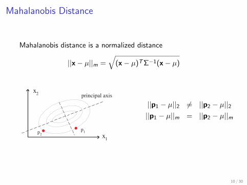
Mahalanobis Distance
Mahalanobis distance is a normalized distance
||x− µ||m =√
(x− µ)TΣ−1(x− µ)
x 1
x 2 principal axis
p 1 p
2
||p1 − µ||2 6= ||p2 − µ||2||p1 − µ||m = ||p2 − µ||m
10 / 30
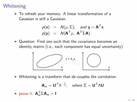
Whitening
I To refresh your memory: A linear transformation of aGaussian is still a Gaussian.
p(x) = N(µ,Σ), and y = ATx
p(y) = N(ATµ, ATΣA)
I Question: Find one such that the covariance becomes anidentity matrix (i.e., each component has equal uncertainty)
y = A w x
x y
I Whitening is a transform that de-couples the correlation.
Aw = UTΛ−12 , where Σ = UTΛU
I prove it: ATwΣAw = I
11 / 30
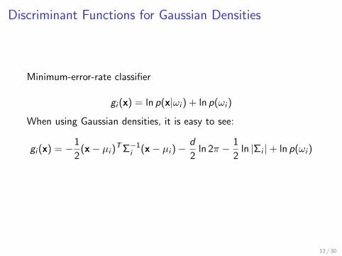
Discriminant Functions for Gaussian Densities
Minimum-error-rate classifier
gi (x) = ln p(x|ωi ) + ln p(ωi )
When using Gaussian densities, it is easy to see:
gi (x) = −1
2(x− µi )TΣ−1
i (x− µi )−d
2ln 2π − 1
2ln |Σi |+ ln p(ωi )
12 / 30
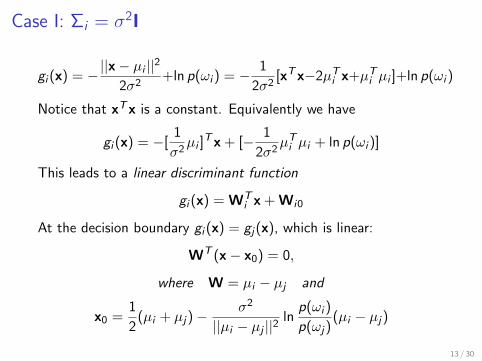
Case I: Σi = σ2I
gi (x) = −||x− µi ||2
2σ2+ln p(ωi ) = − 1
2σ2[xTx−2µTi x+µTi µi ]+ln p(ωi )
Notice that xTx is a constant. Equivalently we have
gi (x) = −[1
σ2µi ]
Tx + [− 1
2σ2µTi µi + ln p(ωi )]
This leads to a linear discriminant function
gi (x) = WTi x + Wi0
At the decision boundary gi (x) = gj(x), which is linear:
WT (x− x0) = 0,
where W = µi − µj and
x0 =1
2(µi + µj)−
σ2
||µi − µj ||2ln
p(ωi )
p(ωj)(µi − µj)
13 / 30
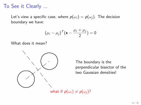
To See it Clearly ...
Let’s view a specific case, where p(ωi ) = p(ωj). The decisionboundary we have:
(µi − µj)T (x−µi + µj
2) = 0
What does it mean?
The boundary is theperpendicular bisector of thetwo Gaussian densities!
what if p(ωi ) 6= p(ωj)?
14 / 30
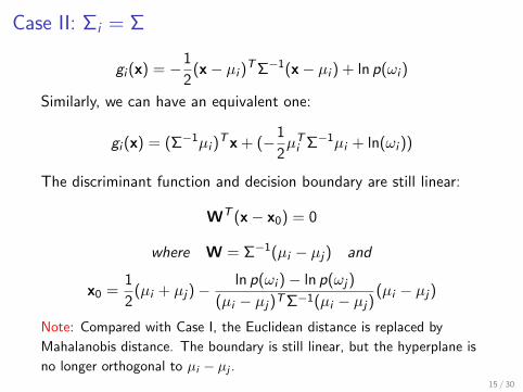
Case II: Σi = Σ
gi (x) = −1
2(x− µi )TΣ−1(x− µi ) + ln p(ωi )
Similarly, we can have an equivalent one:
gi (x) = (Σ−1µi )Tx + (−1
2µTi Σ−1µi + ln(ωi ))
The discriminant function and decision boundary are still linear:
WT (x− x0) = 0
where W = Σ−1(µi − µj) and
x0 =1
2(µi + µj)−
ln p(ωi )− ln p(ωj)
(µi − µj)TΣ−1(µi − µj)(µi − µj)
Note: Compared with Case I, the Euclidean distance is replaced by
Mahalanobis distance. The boundary is still linear, but the hyperplane is
no longer orthogonal to µi − µj .15 / 30
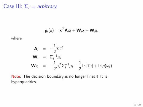
Case III: Σi = arbitrary
gi (x) = xTAix + Wix + Wi0,
where
Ai = −1
2Σ−1i
Wi = Σ−1i µi
Wi0 = −1
2µTi Σ−1
i µi −1
2ln |Σi |+ ln p(ωi )
Note: The decision boundary is no longer linear! It isbyperquadrics.
16 / 30
Outline
Bayesian Decision Theory
Bayesian Classification
Maximum Likelihood Estimation and Learning
Bayesian Estimation and Learning
17 / 30
Learning
I Learning means “training”
I i.e., estimating some unknowns from training samplesI Why?
I It is very difficult to specify these unknownsI Hopefully, these unknowns can be recovered from examples
given
18 / 30
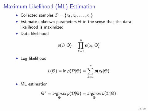
Maximum Likelihood (ML) Estimation
I Collected samples D = {x1, x2, . . . , xn}I Estimate unknown parameters Θ in the sense that the data
likelihood is maximized
I Data likelihood
p(D|Θ) =n∏
k=1
p(xk |Θ)
I Log likelihood
L(Θ) = ln p(D|Θ) =n∑
k=1
p(xk |Θ)
I ML estimation
Θ∗ = argmaxΘ
p(D|Θ) = argmaxΘ
L(D|Θ)
19 / 30
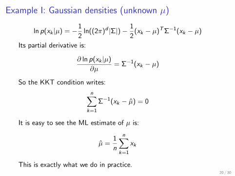
Example I: Gaussian densities (unknown µ)
ln p(xk |µ) = −1
2ln((2π)d |Σ|)− 1
2(xk − µ)TΣ−1(xk − µ)
Its partial derivative is:
∂ ln p(xk |µ)
∂µ= Σ−1(xk − µ)
So the KKT condition writes:
n∑k=1
Σ−1(xk − µ̂) = 0
It is easy to see the ML estimate of µ is:
µ̂ =1
n
n∑k=1
xk
This is exactly what we do in practice.20 / 30
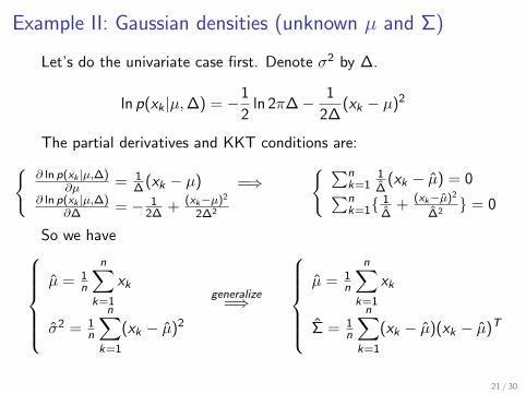
Example II: Gaussian densities (unknown µ and Σ)
Let’s do the univariate case first. Denote σ2 by ∆.
ln p(xk |µ,∆) = −1
2ln 2π∆− 1
2∆(xk − µ)2
The partial derivatives and KKT conditions are:{∂ ln p(xk |µ,∆)
∂µ = 1∆ (xk − µ)
∂ ln p(xk |µ,∆)∂∆ = − 1
2∆ + (xk−µ)2
2∆2
=⇒{ ∑n
k=11∆̂
(xk − µ̂) = 0∑nk=1{
1∆̂
+ (xk−µ̂)2
∆̂2} = 0
So we haveµ̂ = 1
n
n∑k=1
xk
σ̂2 = 1n
n∑k=1
(xk − µ̂)2
generalize=⇒
µ̂ = 1
n
n∑k=1
xk
Σ̂ = 1n
n∑k=1
(xk − µ̂)(xk − µ̂)T
21 / 30
Outline
Bayesian Decision Theory
Bayesian Classification
Maximum Likelihood Estimation and Learning
Bayesian Estimation and Learning
22 / 30
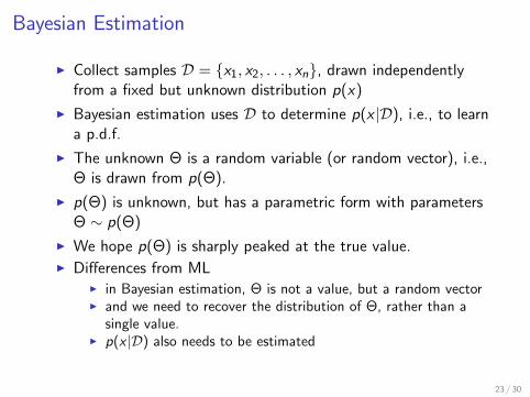
Bayesian Estimation
I Collect samples D = {x1, x2, . . . , xn}, drawn independentlyfrom a fixed but unknown distribution p(x)
I Bayesian estimation uses D to determine p(x |D), i.e., to learna p.d.f.
I The unknown Θ is a random variable (or random vector), i.e.,Θ is drawn from p(Θ).
I p(Θ) is unknown, but has a parametric form with parametersΘ ∼ p(Θ)
I We hope p(Θ) is sharply peaked at the true value.I Differences from ML
I in Bayesian estimation, Θ is not a value, but a random vectorI and we need to recover the distribution of Θ, rather than a
single value.I p(x |D) also needs to be estimated
23 / 30
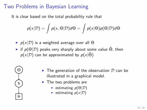
Two Problems in Bayesian Learning
It is clear based on the total probability rule that
p(x |D) =
∫p(x ,Θ|D)dΘ =
∫p(x |Θ)p(Θ|D)dΘ
I p(x |D) is a weighted average over all Θ
I if p(Θ|D) peaks very sharply about some value Θ̂, thenp(x |D) can be approximated by p(x |Θ̂)
X
D
I The generation of the observation D can beillustrated in a graphical model.
I The two problems areI estimating p(Θ|D)I estimating p(x |D)
24 / 30
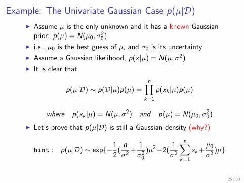
Example: The Univariate Gaussian Case p(µ|D)
I Assume µ is the only unknown and it has a known Gaussianprior: p(µ) = N(µ0, σ
20).
I i.e., µ0 is the best guess of µ, and σ0 is its uncertainty
I Assume a Gaussian likelihood, p(x |µ) = N(µ, σ2)
I It is clear that
p(µ|D) ∼ p(D|µ)p(µ) =n∏
k=1
p(xk |µ)p(µ)
where p(xk |µ) = N(µ, σ2) and p(µ) = N(µ0, σ20)
I Let’s prove that p(µ|D) is still a Gaussian density (why?)
hint : p(µ|D) ∼ exp{−1
2(
n
σ2+
1
σ20
)µ2−2(1
σ2
n∑k=1
xk +µ0
σ2)µ}
25 / 30
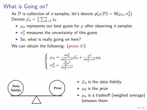
What is Going on?As D is collection of n samples, let’s denote p(µ|D) = N(µn, σ
2n).
Denote µ̄n = 1n
∑nk=1 xk .
I µn represents our best guess for µ after observing n samples
I σ2n measures the uncertainty of this guess
I So, what is really going on here?
We can obtain the following: (prove it!) µn =nσ2
0
nσ20+σ2 µ̄n + σ2
nσ20+σ2µ0
σ2n =
σ20σ
2
nσ20+σ2
Data
fidelity Prior
I µ̄n is the data fidelity
I µ0 is the prior
I µn is a tradeoff (weighed average)between them
26 / 30
Example: The Univariate Gaussian case p(x |D)
After obtaining the posterior p(µ|D), we can estimate p(x |D)
p(x |D) =
∫p(x |µ)p(µ|D)dµ
It is the convolution of two Gaussian distributions. You can easilyprove: do it!
p(x |D) = N(µn, σ2 + σ2
n)
27 / 30
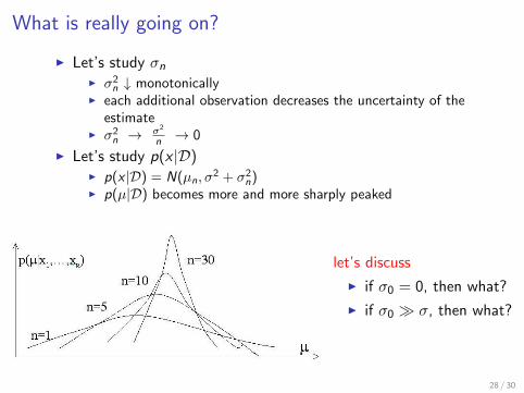
What is really going on?
I Let’s study σnI σ2
n ↓ monotonicallyI each additional observation decreases the uncertainty of the
estimateI σ2
n → σ2
n → 0
I Let’s study p(x |D)I p(x |D) = N(µn, σ
2 + σ2n)
I p(µ|D) becomes more and more sharply peaked
let’s discuss
I if σ0 = 0, then what?
I if σ0 � σ, then what?
28 / 30
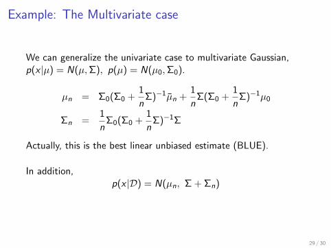
Example: The Multivariate case
We can generalize the univariate case to multivariate Gaussian,p(x |µ) = N(µ,Σ), p(µ) = N(µ0,Σ0).
µn = Σ0(Σ0 +1
nΣ)−1µ̄n +
1
nΣ(Σ0 +
1
nΣ)−1µ0
Σn =1
nΣ0(Σ0 +
1
nΣ)−1Σ
Actually, this is the best linear unbiased estimate (BLUE).
In addition,p(x |D) = N(µn, Σ + Σn)
29 / 30
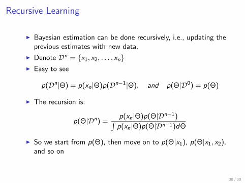
Recursive Learning
I Bayesian estimation can be done recursively, i.e., updating theprevious estimates with new data.
I Denote Dn = {x1, x2, . . . , xn}I Easy to see
p(Dn|Θ) = p(xn|Θ)p(Dn−1|Θ), and p(Θ|D0) = p(Θ)
I The recursion is:
p(Θ|Dn) =p(xn|Θ)p(Θ|Dn−1)∫
p(xn|Θ)p(Θ|Dn−1)dΘ
I So we start from p(Θ), then move on to p(Θ|x1), p(Θ|x1, x2),and so on
30 / 30


![Graphs and polytopes: learning Bayesian networks with LP ...people.csail.mit.edu/tommi/papers/BNstructure_slides.pdf“Fundaci´on Rafael del Pino” Fellow. References [1] Adam Arkin,](https://static.fdocument.org/doc/165x107/5febf0979191e72bac765d5c/graphs-and-polytopes-learning-bayesian-networks-with-lp-aoefundacion-rafael.jpg)