Bayes Net Syntax and Semantics
35
Bayes Net Syntax and Semantics
Transcript of Bayes Net Syntax and Semantics
Bayes Net Syntax and Semantics
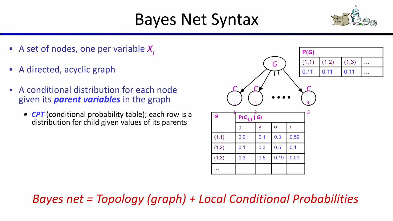
Bayes Net Syntax
▪ A set of nodes, one per variable Xi
▪ A directed, acyclic graph
▪ A conditional distribution for each node given its parent variables in the graph
▪ CPT (conditional probability table); each row is a distribution for child given values of its parents
Bayes net = Topology (graph) + Local Conditional Probabilities
G P(C1,1 | G)
g y o r
(1,1) 0.01 0.1 0.3 0.59
(1,2) 0.1 0.3 0.5 0.1
(1,3) 0.3 0.5 0.19 0.01
…
P(G)(1,1) (1,2) (1,3) …
0.11 0.11 0.11 …G
C
1,
1
C
1,
2
C
3,
3
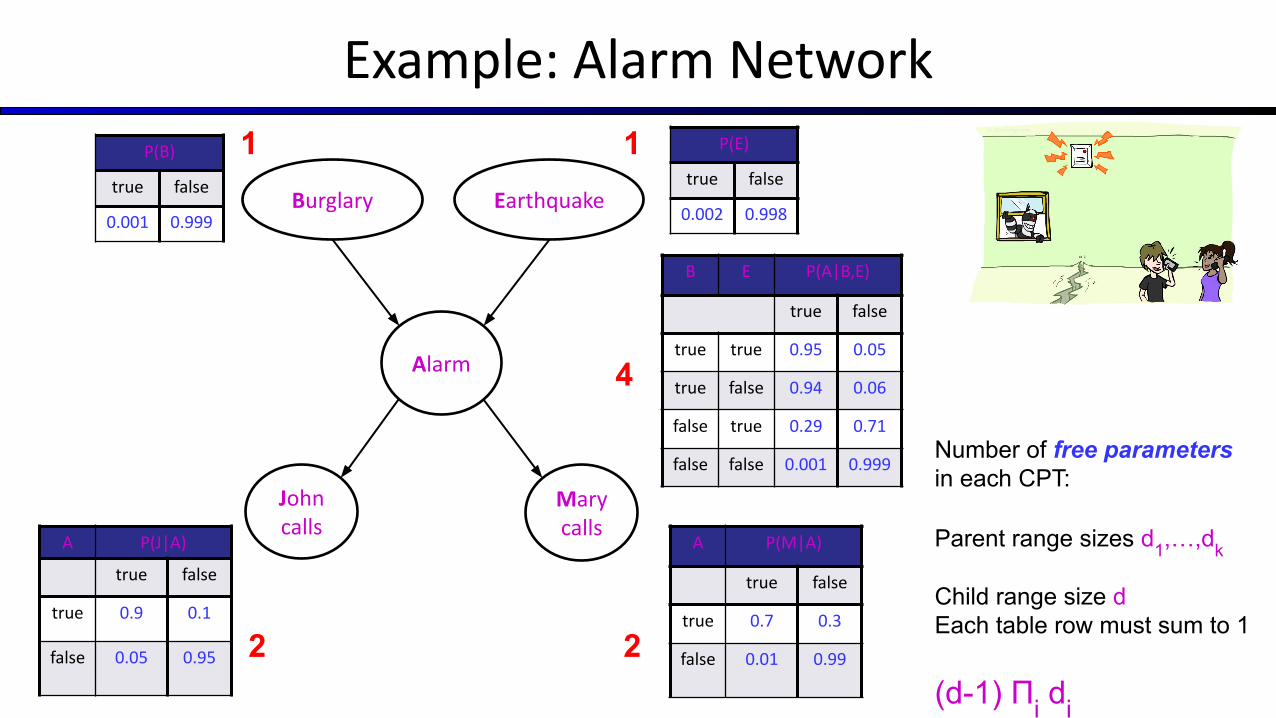
Example: Alarm Network
Burglary Earthquake
Alarm
John calls
Mary calls
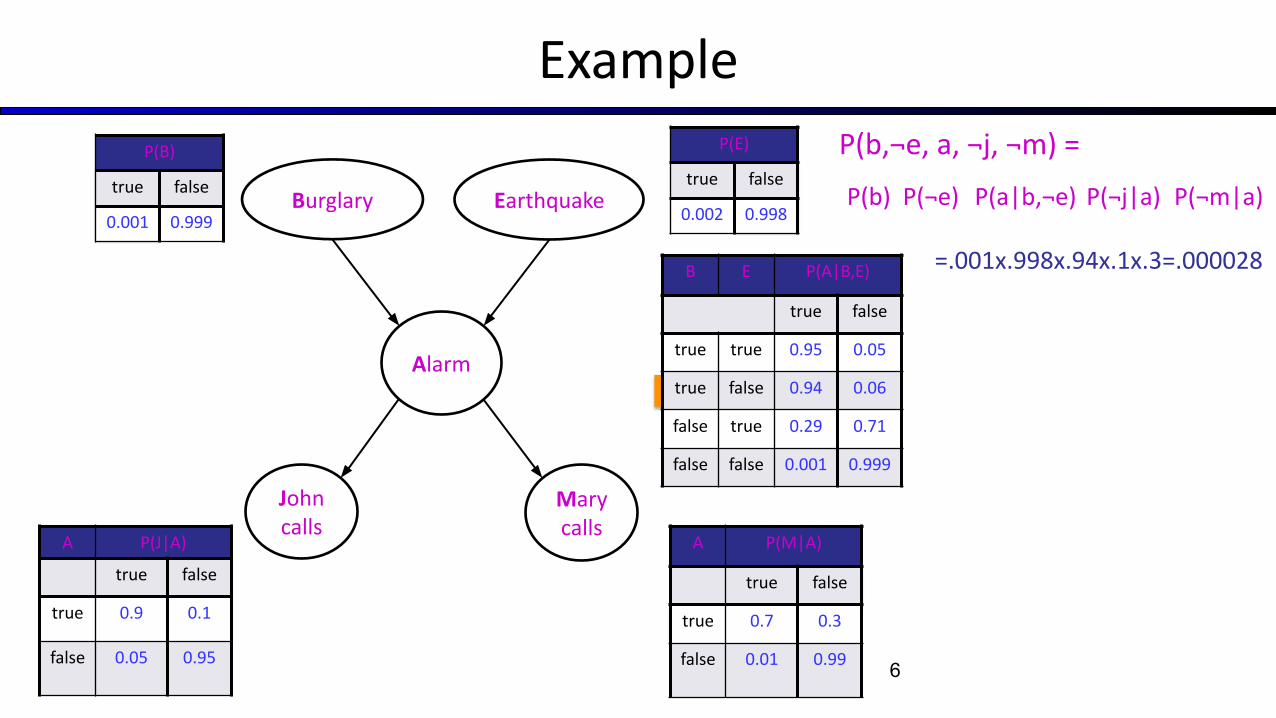
P(B)
true false
0.001 0.999
B E P(A|B,E)
true false
true true 0.95 0.05
true false 0.94 0.06
false true 0.29 0.71
false false 0.001 0.999
A P(J|A)
true false
true 0.9 0.1
false 0.05 0.95
P(E)
true false
0.002 0.998
A P(M|A)
true false
true 0.7 0.3
false 0.01 0.99
Number of free parameters in each CPT:
Parent range sizes d1,…,dk
Child range size d Each table row must sum to 1
(d-1) Πi di
1 1
4
2 2
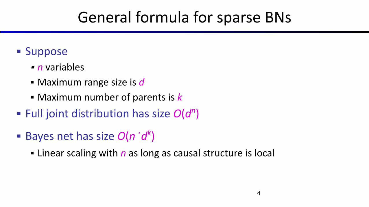
General formula for sparse BNs
▪ Suppose▪ n variables
▪ Maximum range size is d
▪ Maximum number of parents is k
▪ Full joint distribution has size O(dn)
▪ Bayes net has size O(n .dk)
▪ Linear scaling with n as long as causal structure is local
4
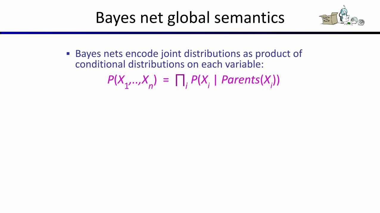
Bayes net global semantics
▪ Bayes nets encode joint distributions as product of conditional distributions on each variable:
P(X1,..,X
n) = ∏
i P(X
i | Parents(X
i))
P(B)
true false
0.001 0.999
Example
P(b,¬e, a, ¬j, ¬m) =
6
B E P(A|B,E)
true false
true true 0.95 0.05
true false 0.94 0.06
false true 0.29 0.71
false false 0.001 0.999
A P(J|A)
true false
true 0.9 0.1
false 0.05 0.95
P(E)
true false
0.002 0.998
A P(M|A)
true false
true 0.7 0.3
false 0.01 0.99
P(b) P(¬e) P(a|b,¬e) P(¬j|a) P(¬m|a)
=.001x.998x.94x.1x.3=.000028
Burglary Earthquake
Alarm
John calls
Mary calls
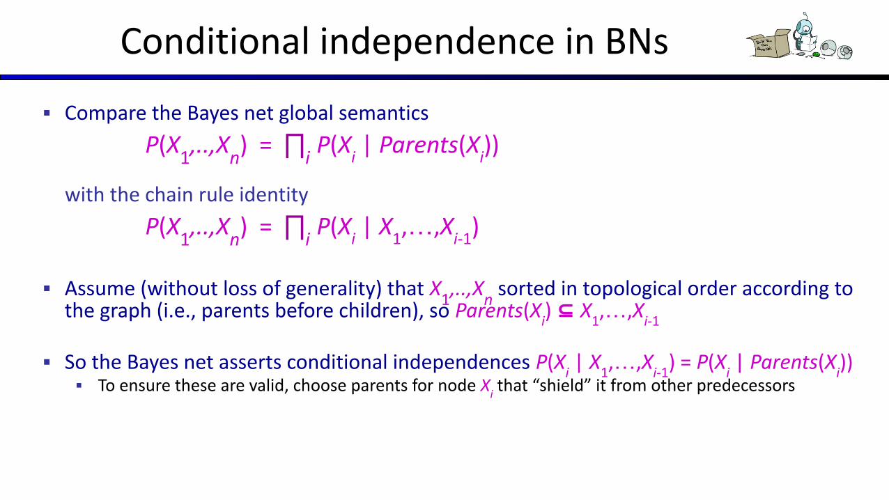
Conditional independence in BNs
▪ Compare the Bayes net global semantics
P(X1,..,X
n) = ∏
i P(X
i | Parents(X
i))
with the chain rule identity
P(X1,..,X
n) = ∏
i P(X
i | X
1,…,X
i-1)
▪ Assume (without loss of generality) that X1,..,X
n sorted in topological order according to
the graph (i.e., parents before children), so Parents(Xi) ⊆ X
1,…,X
i-1
▪ So the Bayes net asserts conditional independences P(Xi | X
1,…,X
i-1) = P(X
i | Parents(X
i))
▪ To ensure these are valid, choose parents for node Xi that “shield” it from other predecessors
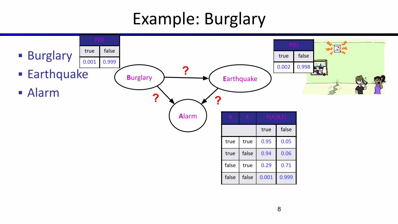
Example: Burglary
▪ Burglary
▪ Earthquake
▪ Alarm
8
Burglary Earthquake
Alarm
?
??
P(B)
true false
0.001 0.999
B E P(A|B,E)
true false
true true 0.95 0.05
true false 0.94 0.06
false true 0.29 0.71
false false 0.001 0.999
P(E)
true false
0.002 0.998
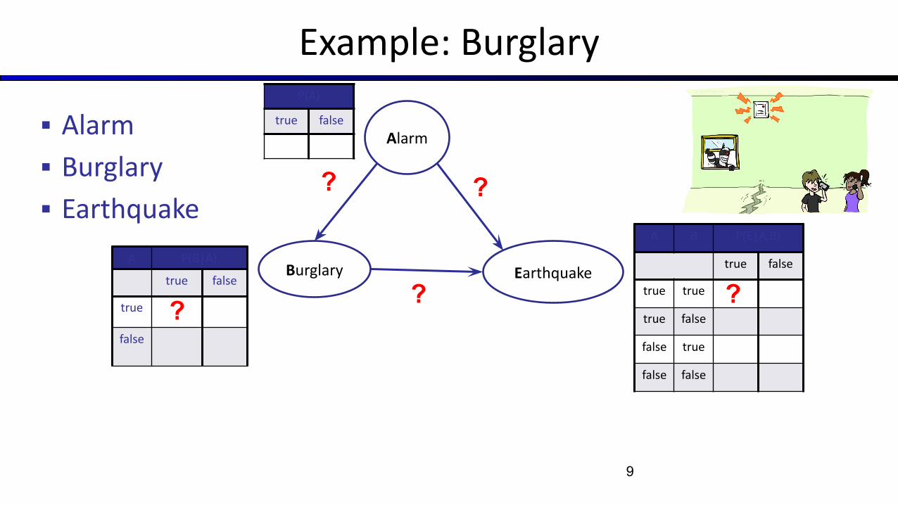
Example: Burglary
▪ Alarm
▪ Burglary
▪ Earthquake
9
Burglary Earthquake
Alarm
?
?
?
P(A)
true false
A B P(E|A,B)
true false
true true
true false
false true
false false
A P(B|A)
true false
true
false
? ?
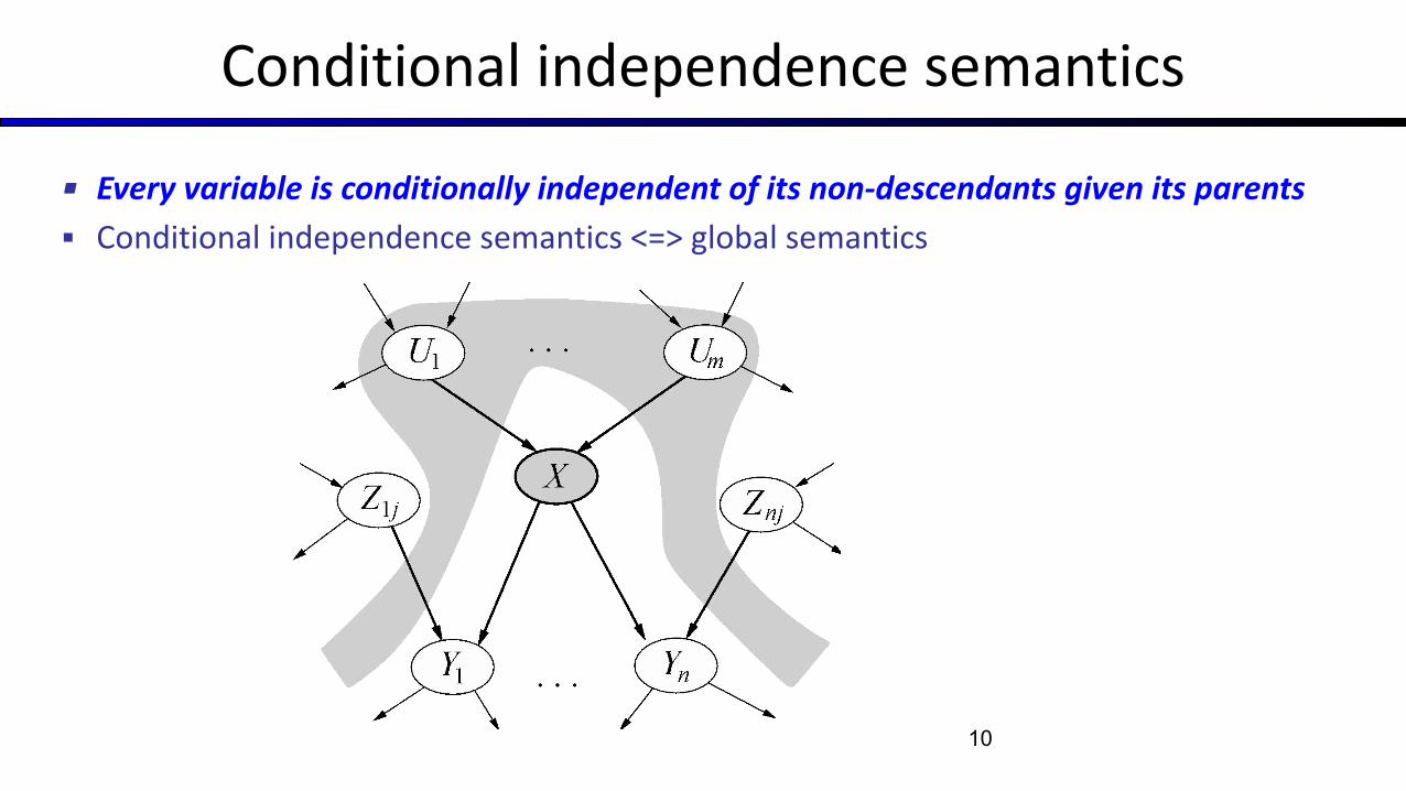
Conditional independence semantics
▪ Every variable is conditionally independent of its non-descendants given its parents
▪ Conditional independence semantics <=> global semantics
10
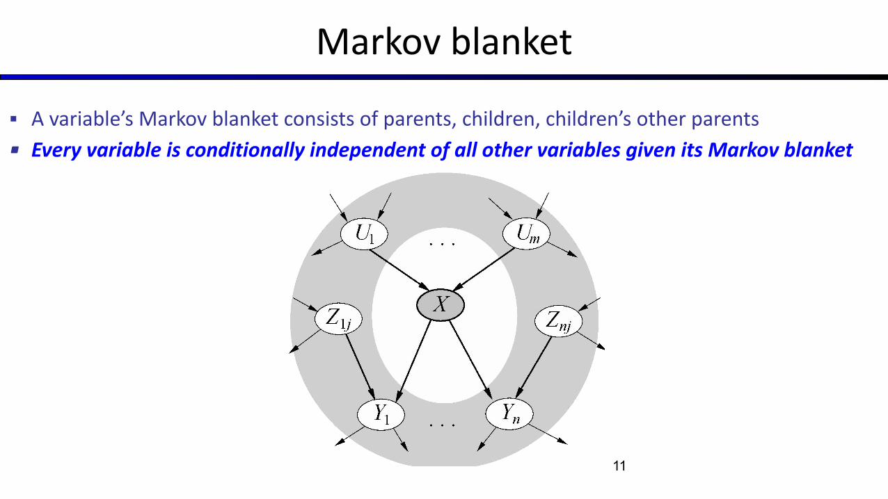
Markov blanket
▪ A variable’s Markov blanket consists of parents, children, children’s other parents
▪ Every variable is conditionally independent of all other variables given its Markov blanket
11
Summary
▪ Independence and conditional independence are important forms of probabilistic knowledge
▪ Bayes net encode joint distributions efficiently by taking advantage of conditional independence▪ Global joint probability = product of local conditionals▪ Local causality => exponential reduction in total size
CS 188: Artificial Intelligence
Bayes Nets: Exact Inference
Instructor: Stuart Russell and Dawn Song --- University of California, Berkeley
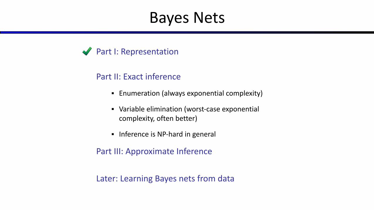
Bayes Nets
Part I: Representation
Part II: Exact inference
▪ Enumeration (always exponential complexity)
▪ Variable elimination (worst-case exponential complexity, often better)
▪ Inference is NP-hard in general
Part III: Approximate Inference
Later: Learning Bayes nets from data
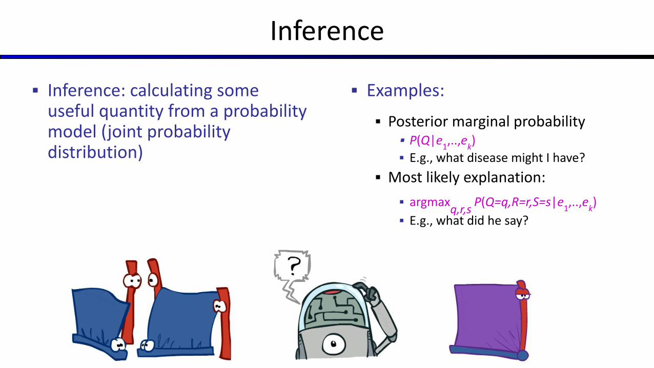
▪ Examples:
▪ Posterior marginal probability▪ P(Q|e
1,..,e
k)
▪ E.g., what disease might I have?
▪ Most likely explanation:
▪ argmaxq,r,s
P(Q=q,R=r,S=s|e1,..,e
k)
▪ E.g., what did he say?
Inference
▪ Inference: calculating some useful quantity from a probability model (joint probability distribution)
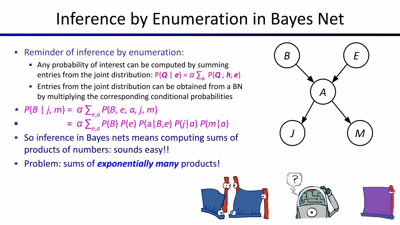
Inference by Enumeration in Bayes Net
▪ Reminder of inference by enumeration:▪ Any probability of interest can be computed by summing
entries from the joint distribution: P(Q | e) = α ∑h P(Q , h,
e)
▪ Entries from the joint distribution can be obtained from a BN by multiplying the corresponding conditional probabilities
▪ P(B | j, m) = α ∑e,a
P(B, e, a, j, m)
▪ = α ∑e,a
P(B) P(e) P(a|B,e) P(j|a) P(m|a)
▪ So inference in Bayes nets means computing sums of products of numbers: sounds easy!!
▪ Problem: sums of exponentially many products!
B E
A
MJ
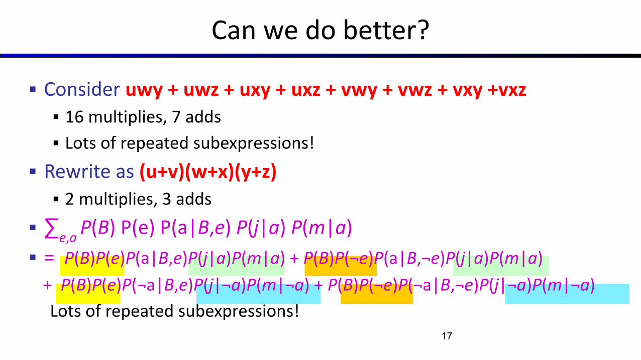
Can we do better?
▪ Consider uwy + uwz + uxy + uxz + vwy + vwz + vxy +vxz ▪ 16 multiplies, 7 adds
▪ Lots of repeated subexpressions!
▪ Rewrite as (u+v)(w+x)(y+z)▪ 2 multiplies, 3 adds
▪ ∑e,a
P(B) P(e) P(a|B,e) P(j|a) P(m|a)
▪ = P(B)P(e)P(a|B,e)P(j|a)P(m|a) + P(B)P(¬e)P(a|B,¬e)P(j|a)P(m|a)
+ P(B)P(e)P(¬a|B,e)P(j|¬a)P(m|¬a) + P(B)P(¬e)P(¬a|B,¬e)P(j|¬a)P(m|¬a)
Lots of repeated subexpressions!17
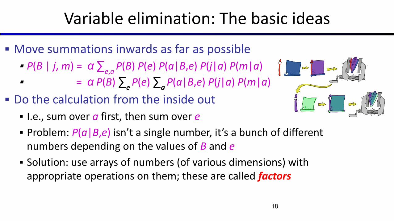
Variable elimination: The basic ideas
▪ Move summations inwards as far as possible▪ P(B | j, m) = α ∑
e,a P(B) P(e) P(a|B,e) P(j|a) P(m|a)
▪ = α P(B) ∑e
P(e) ∑a
P(a|B,e) P(j|a) P(m|a)
▪ Do the calculation from the inside out▪ I.e., sum over a first, then sum over e
▪ Problem: P(a|B,e) isn’t a single number, it’s a bunch of different numbers depending on the values of B and e
▪ Solution: use arrays of numbers (of various dimensions) with appropriate operations on them; these are called factors
18
Factor Zoo
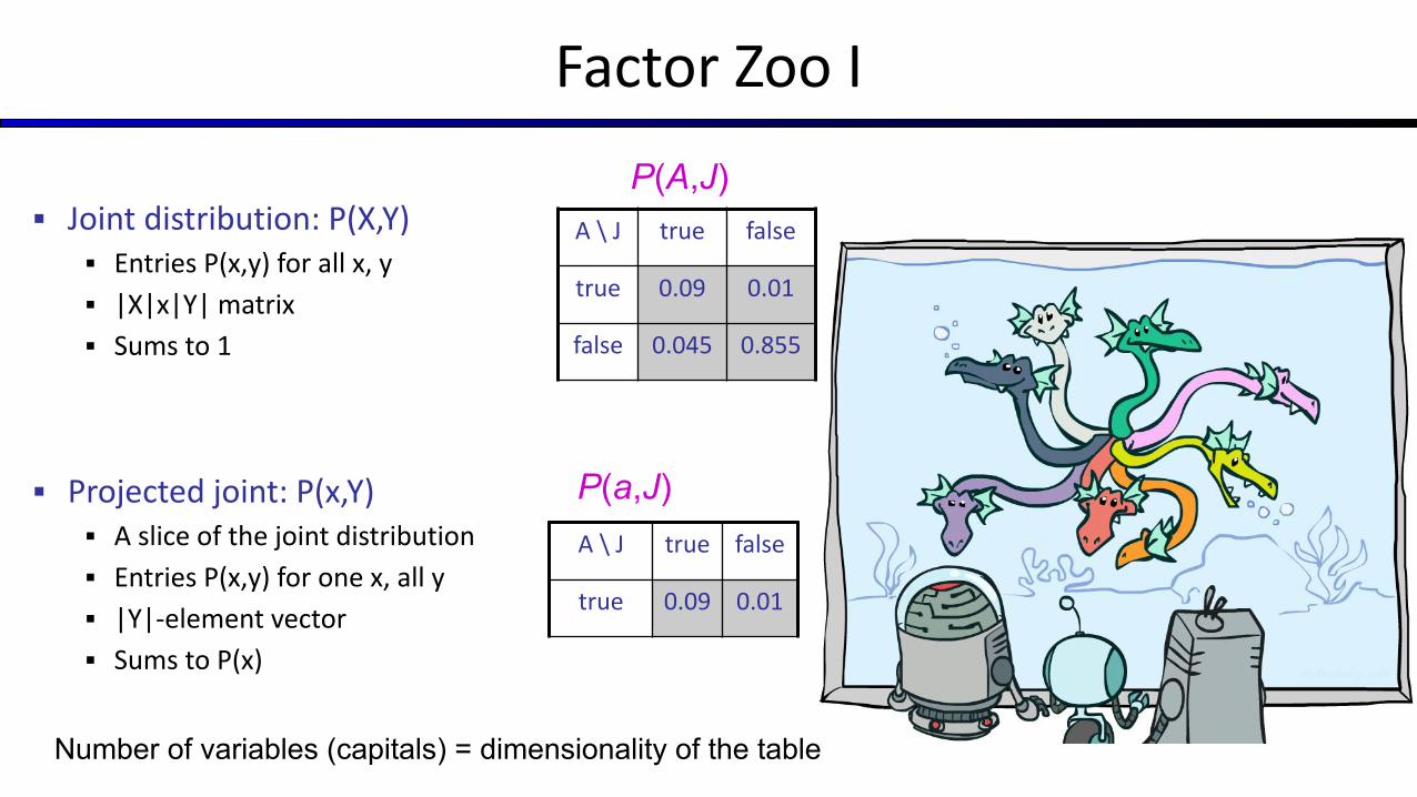
Factor Zoo I
▪ Joint distribution: P(X,Y)▪ Entries P(x,y) for all x, y
▪ |X|x|Y| matrix
▪ Sums to 1
▪ Projected joint: P(x,Y)▪ A slice of the joint distribution
▪ Entries P(x,y) for one x, all y
▪ |Y|-element vector
▪ Sums to P(x)
A \ J true false
true 0.09 0.01
false 0.045 0.855
P(A,J)
P(a,J)
Number of variables (capitals) = dimensionality of the table
A \ J true false
true 0.09 0.01
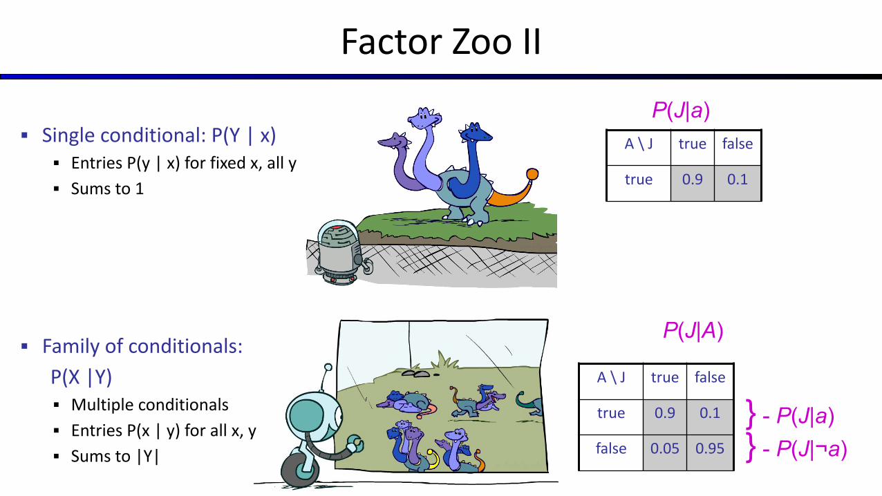
Factor Zoo II
▪ Single conditional: P(Y | x)▪ Entries P(y | x) for fixed x, all y
▪ Sums to 1
▪ Family of conditionals:
P(X |Y)▪ Multiple conditionals
▪ Entries P(x | y) for all x, y
▪ Sums to |Y|
A \ J true false
true 0.9 0.1
P(J|a)
A \ J true false
true 0.9 0.1
false 0.05 0.95
P(J|A)
} - P(J|a)} - P(J|¬a)
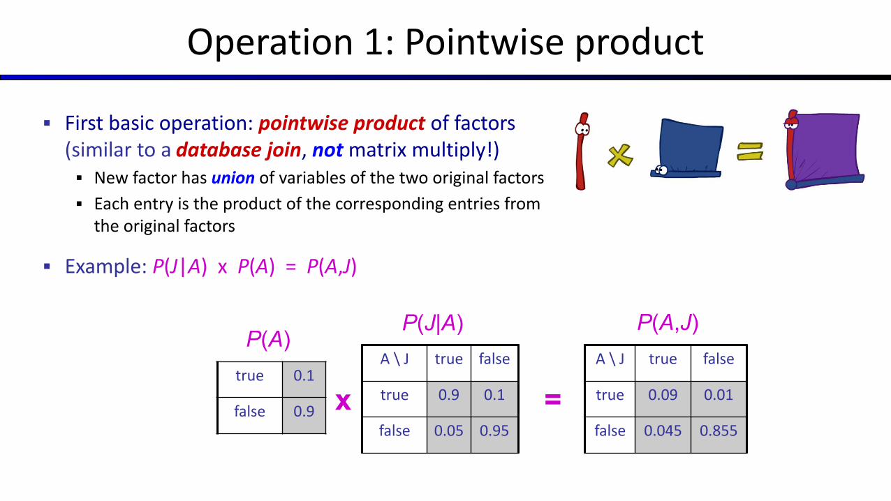
Operation 1: Pointwise product
▪ First basic operation: pointwise product of factors (similar to a database join, not matrix multiply!)▪ New factor has union of variables of the two original factors
▪ Each entry is the product of the corresponding entries from the original factors
▪ Example: P(J|A) x P(A) = P(A,J)
P(J|A)P(A)
P(A,J)A \ J true false
true 0.09 0.01
false 0.045 0.855
A \ J true false
true 0.9 0.1
false 0.05 0.95
true 0.1
false 0.9 x =
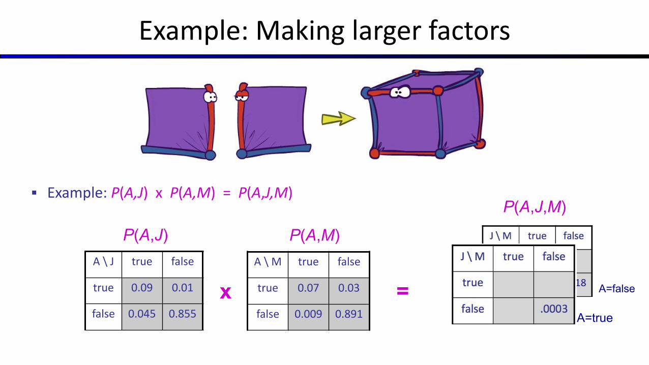
Example: Making larger factors
▪ Example: P(A,J) x P(A,M) = P(A,J,M)
P(A,J)A \ J true false
true 0.09 0.01
false 0.045 0.855
x =
P(A,M)A \ M true false
true 0.07 0.03
false 0.009 0.891 A=true
A=false
P(A,J,M)
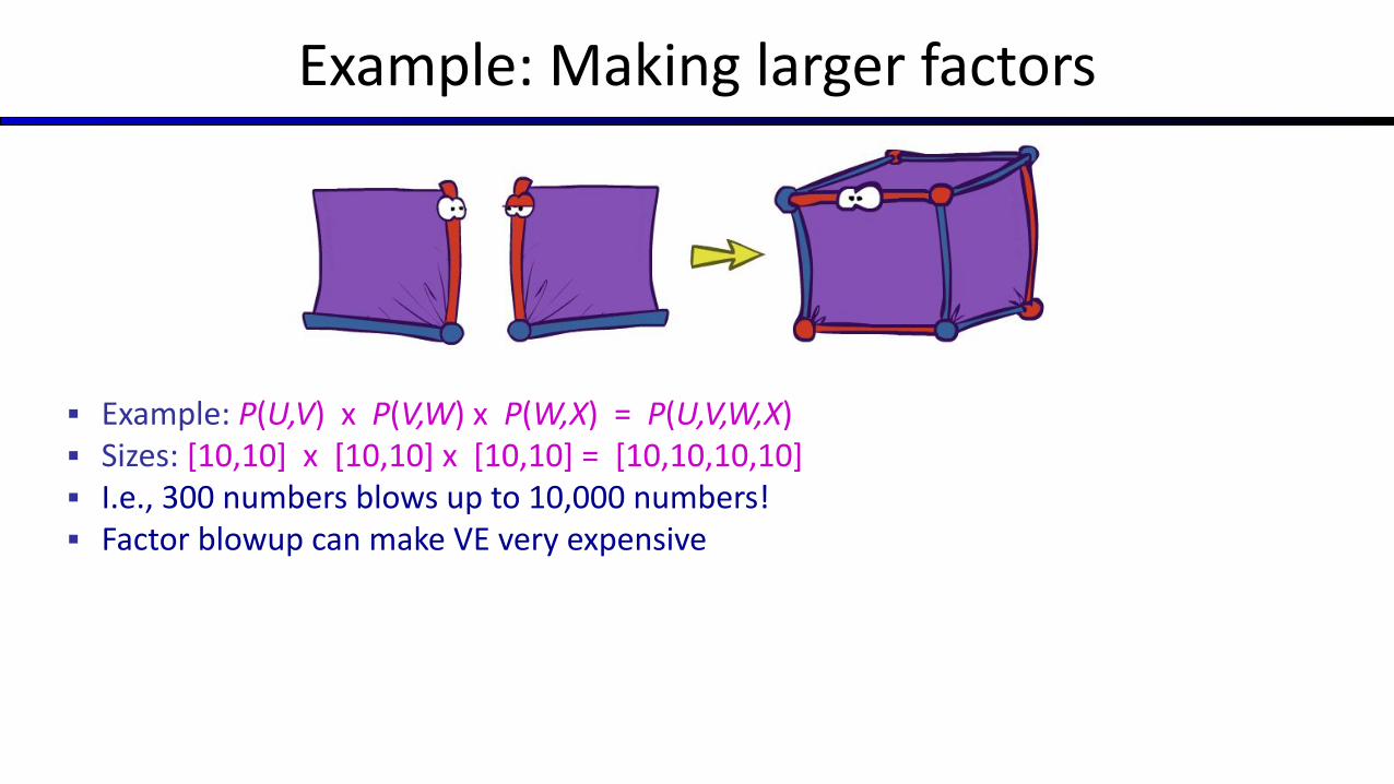
Example: Making larger factors
▪ Example: P(U,V) x P(V,W) x P(W,X) = P(U,V,W,X)▪ Sizes: [10,10] x [10,10] x [10,10] = [10,10,10,10] ▪ I.e., 300 numbers blows up to 10,000 numbers!▪ Factor blowup can make VE very expensive
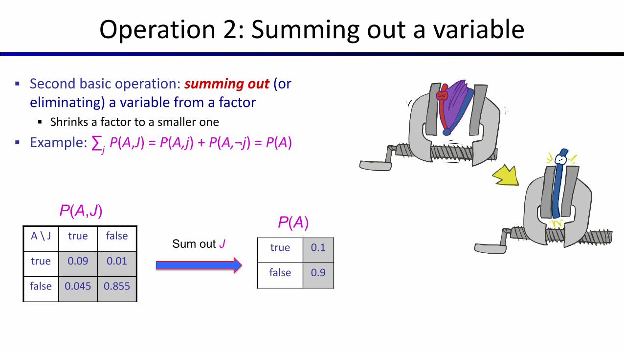
Operation 2: Summing out a variable
▪ Second basic operation: summing out (or eliminating) a variable from a factor▪ Shrinks a factor to a smaller one
▪ Example: ∑j
P(A,J) = P(A,j) + P(A,¬j) = P(A)
A \ J true false
true 0.09 0.01
false 0.045 0.855
true 0.1
false 0.9
P(A)P(A,J)
Sum out J
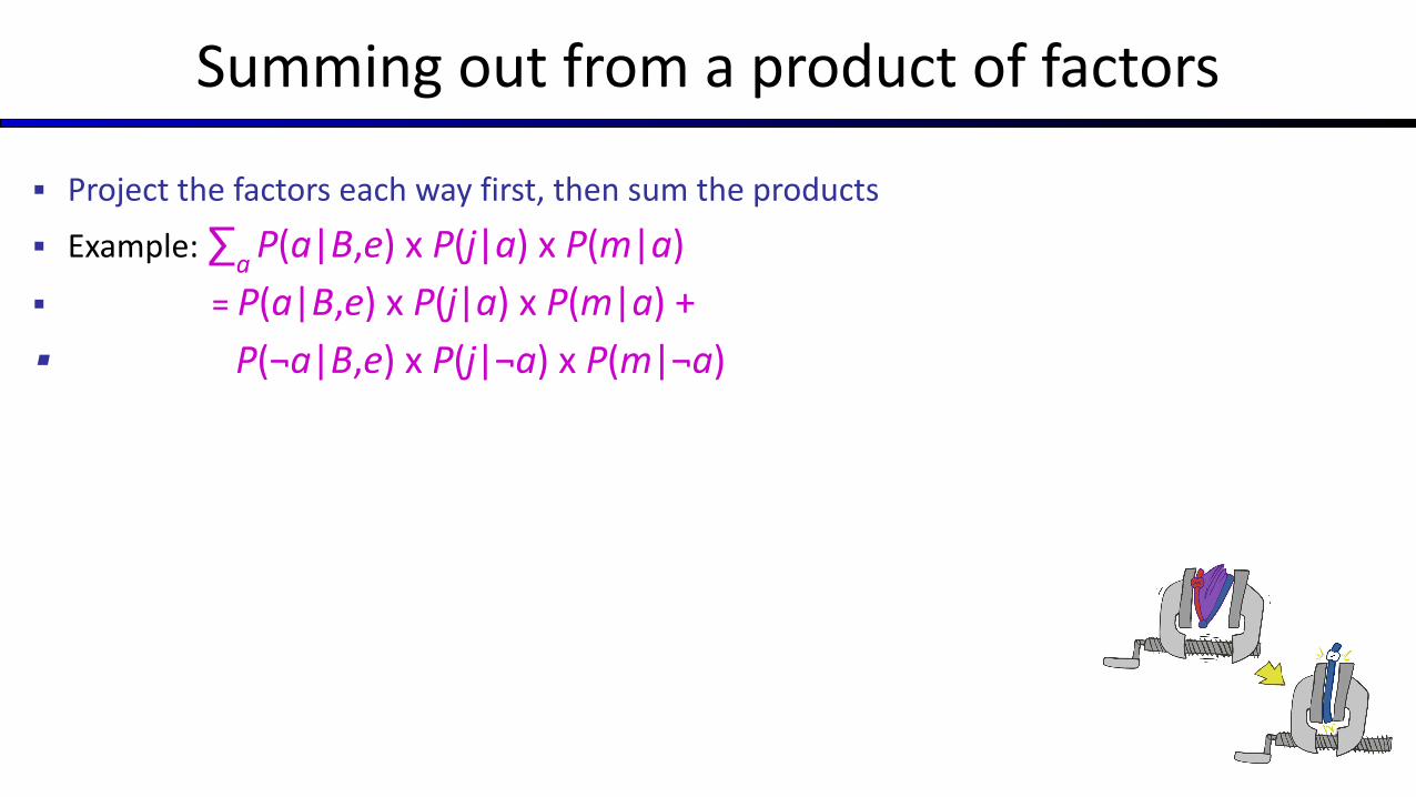
Summing out from a product of factors
▪ Project the factors each way first, then sum the products
▪ Example: ∑a
P(a|B,e) x P(j|a) x P(m|a)
▪ = P(a|B,e) x P(j|a) x P(m|a) +
▪ P(¬a|B,e) x P(j|¬a) x P(m|¬a)
Variable Elimination

Variable Elimination
▪ Query: P(Q|E1=e
1,.., E
k=e
k)
▪ Start with initial factors:▪ Local CPTs (but instantiated by evidence)
▪ While there are still hidden variables (not Q or evidence):▪ Pick a hidden variable H
j
▪ Eliminate (sum out) Hj from the product of all
factors mentioning Hj
▪ Join all remaining factors and normalizeX α
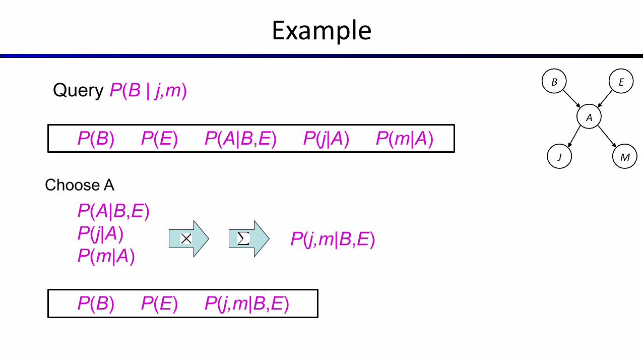
Example
Choose A
P(B) P(E) P(A|B,E) P(j|A) P(m|A)
Query P(B | j,m)
P(A|B,E) P(j|A)P(m|A)
P(j,m|B,E)
P(B) P(E) P(j,m|B,E)
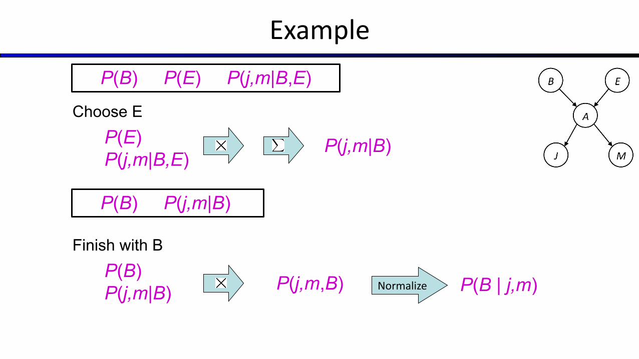
Example
Normalize
Choose EP(E) P(j,m|B,E)
P(j,m|B)
P(B) P(E) P(j,m|B,E)
Finish with BP(B) P(j,m|B) P(j,m,B)
P(B) P(j,m|B)
P(B | j,m)
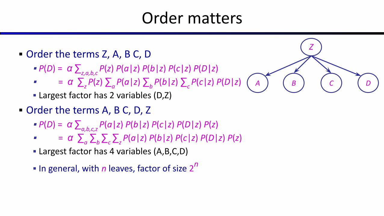
Order matters
▪ Order the terms Z, A, B C, D▪ P(D) = α ∑
z,a,b,c P(z) P(a|z) P(b|z) P(c|z) P(D|z)
▪ = α ∑z P(z) ∑
a P(a|z) ∑
b P(b|z) ∑
c P(c|z) P(D|z)
▪ Largest factor has 2 variables (D,Z)
▪ Order the terms A, B C, D, Z▪ P(D) = α ∑
a,b,c,z P(a|z) P(b|z) P(c|z) P(D|z) P(z)
▪ = α ∑a ∑
b ∑
c ∑
z P(a|z) P(b|z) P(c|z) P(D|z) P(z)
▪ Largest factor has 4 variables (A,B,C,D)
▪ In general, with n leaves, factor of size 2n
D
Z
A B C
VE: Computational and Space Complexity
▪ The computational and space complexity of variable elimination is determined by the largest factor (and it’s space that kills you)
▪ The elimination ordering can greatly affect the size of the largest factor. ▪ E.g., previous slide’s example 2n vs. 2
▪ Does there always exist an ordering that only results in small factors?▪ No!
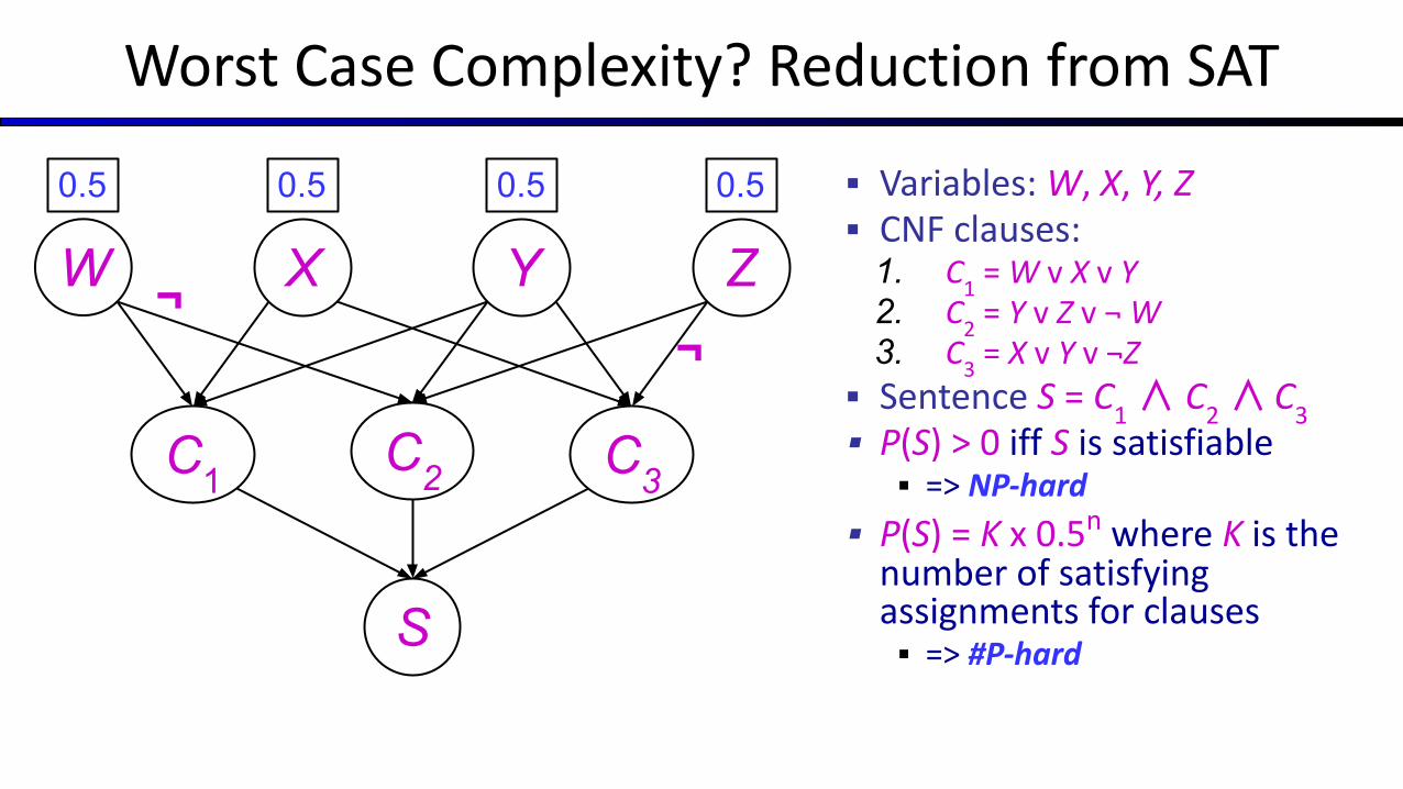
Worst Case Complexity? Reduction from SAT
▪ Variables: W, X, Y, Z▪ CNF clauses:
1. C1 = W v X v Y
2. C2 = Y v Z v ¬ W
3. C3 = X v Y v ¬Z
▪ Sentence S = C1 ∧ C
2 ∧
C
3▪ P(S) > 0 iff S is satisfiable▪ => NP-hard
▪ P(S) = K x 0.5n where K is the number of satisfying assignments for clauses▪ => #P-hard
S
C1 C2 C3
¬ ¬ W X Y Z
0.5 0.50.50.5
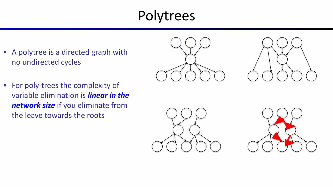
Polytrees
▪ A polytree is a directed graph with no undirected cycles
▪ For poly-trees the complexity of variable elimination is linear in the network size if you eliminate from the leave towards the roots
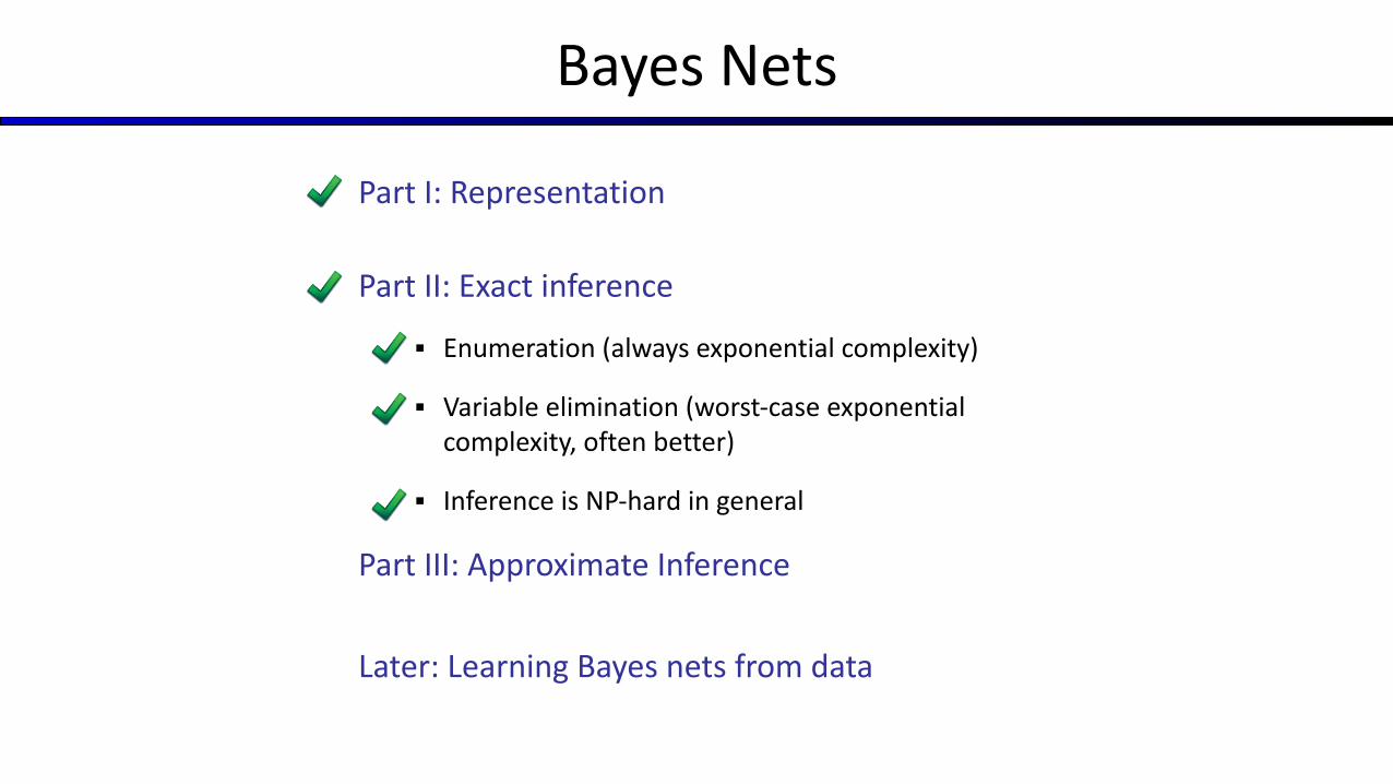
Bayes Nets
Part I: Representation
Part II: Exact inference
▪ Enumeration (always exponential complexity)
▪ Variable elimination (worst-case exponential complexity, often better)
▪ Inference is NP-hard in general
Part III: Approximate Inference
Later: Learning Bayes nets from data