Basic Types of Coarse-Graining II - UT Mathematics
60
Basic Types of Coarse-Graining II Alexander N. Gorban University of Leicester, Leicester LE1 7RH, UK [email protected] Summary. We consider two basic types of coarse-graining: the Ehrenfests’ coarse- graining and its extension to a general principle of non-equilibrium thermodynamics, and the coarse-graining based on uncertainty of dynamical models and ε-motions (orbits). Non-technical discussion of basic notions and main coarse-graining theo- rems are presented: the theorem about entropy overproduction for the Ehrenfests’ coarse-graining and its generalizations, both for conservative and for dissipative sys- tems, and the theorems about stable properties and the Smale order for ε-motions of general dynamical systems including structurally unstable systems. Computational kinetic models of macroscopic dynamics are considered. We construct a theoreti- cal basis for these kinetic models using generalizations of the Ehrenfests’ coarse- graining. General theory of reversible regularization and filtering semigroups in ki- netics is presented, both for linear and non-linear filters. We obtain explicit expres- sions and entropic stability conditions for filtered equations. A brief discussion of coarse-graining by rounding and by small noise is also presented. 1 Introduction Almost a century ago, Paul and Tanya Ehrenfest in their paper for scientific Encyclopedia [1] introduced a special operation, the coarse-graining. This op- eration transforms a probability density in phase space into a “coarse-grained” density, that is a piece-wise constant function, a result of density averaging in cells. The size of cells is assumed to be small, but finite, and does not tend to zero. The coarse-graining models uncontrollable impact of surrounding (of a thermostat, for example) onto ensemble of mechanical systems. To understand reasons for introduction of this new notion, let us take a phase drop, that is, an ensemble of mechanical systems with constant probabil- ity density localized in a small domain of phase space. Let us watch evolution of this drop in time according to the Liouville equation. After a long time, the shape of the drop may be very complicated, but the density value remains the same, and this drop remains “oil in water.” The ensemble can tend to the equilibrium in the weak sense only: average value of any continuous function
Transcript of Basic Types of Coarse-Graining II - UT Mathematics
Basic Types of Coarse-Graining II
Alexander N. Gorban
University of Leicester, Leicester LE1 7RH, UK [email protected]
Summary. We consider two basic types of coarse-graining: the Ehrenfests’ coarse-graining and its extension to a general principle of non-equilibrium thermodynamics,and the coarse-graining based on uncertainty of dynamical models and ε-motions(orbits). Non-technical discussion of basic notions and main coarse-graining theo-rems are presented: the theorem about entropy overproduction for the Ehrenfests’coarse-graining and its generalizations, both for conservative and for dissipative sys-tems, and the theorems about stable properties and the Smale order for ε-motions ofgeneral dynamical systems including structurally unstable systems. Computationalkinetic models of macroscopic dynamics are considered. We construct a theoreti-cal basis for these kinetic models using generalizations of the Ehrenfests’ coarse-graining. General theory of reversible regularization and filtering semigroups in ki-netics is presented, both for linear and non-linear filters. We obtain explicit expres-sions and entropic stability conditions for filtered equations. A brief discussion ofcoarse-graining by rounding and by small noise is also presented.
1 Introduction
Almost a century ago, Paul and Tanya Ehrenfest in their paper for scientificEncyclopedia [1] introduced a special operation, the coarse-graining. This op-eration transforms a probability density in phase space into a “coarse-grained”density, that is a piece-wise constant function, a result of density averaging incells. The size of cells is assumed to be small, but finite, and does not tend tozero. The coarse-graining models uncontrollable impact of surrounding (of athermostat, for example) onto ensemble of mechanical systems.
To understand reasons for introduction of this new notion, let us take aphase drop, that is, an ensemble of mechanical systems with constant probabil-ity density localized in a small domain of phase space. Let us watch evolutionof this drop in time according to the Liouville equation. After a long time,the shape of the drop may be very complicated, but the density value remainsthe same, and this drop remains “oil in water.” The ensemble can tend to theequilibrium in the weak sense only: average value of any continuous function
2 Alexander N. Gorban
a)
Phase space
with cells
Motion of distribution
Distribution
averaging in cells
Co
ars
e-g
rain
ed
den
sit
y
Mechanical motion of ensemble, S=const
Coarse-graining, S increases
b)
Mechanical motion of
ensemble, S=const
Coarse-graining,
S increases
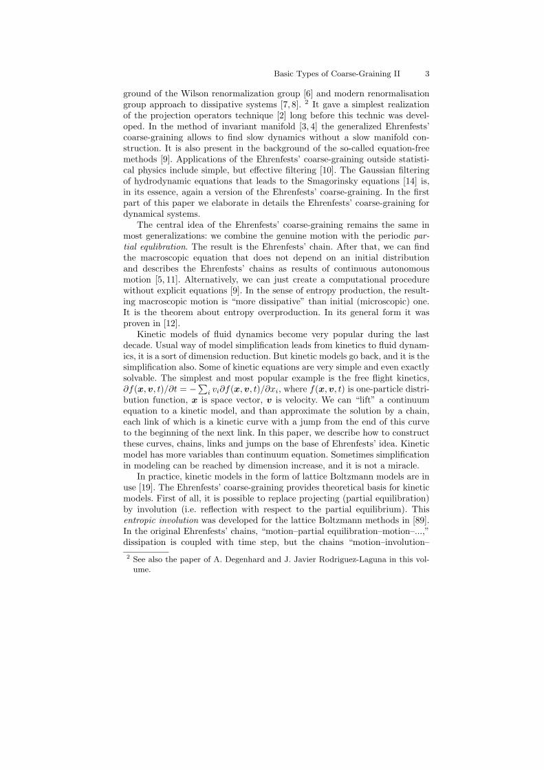
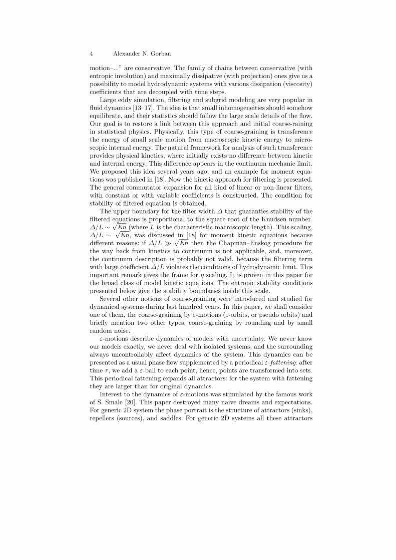
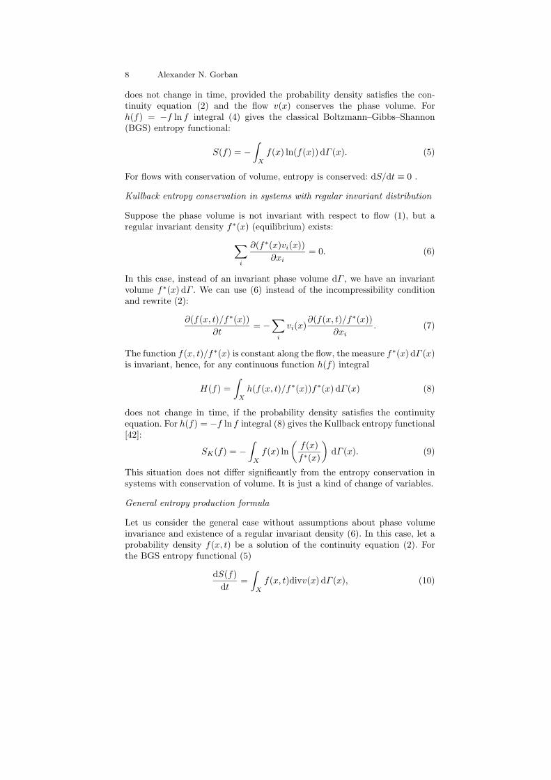
Fig. 1. The Ehrenfests’ coarse-graining: two “motion – coarse-graining” cycles in1D (a, values of probability density are presented by the height of the columns)and one such cycle in 2D (b, values of probability density are presented by hatchingdensity).
tends to its equilibrium value, but the entropy of the distribution remainsconstant. Nevertheless, if we divide the phase space into cells and supplementthe mechanical motion by the periodical averaging in cells (this is the Ehren-fests’ idea of coarse-graining), then the entropy increases, and the distributiondensity tends uniformly to the equilibrium. This periodical coarse-graining isillustrated by Fig. 1 for one-dimensional (1D)1 and two-dimensional (2D)phase spaces.
Recently, we can find the idea of coarse-graining everywhere in statisti-cal physics (both equilibrium and non-equilibrium). For example, it is thecentral idea of the Kadanoff transformation, and can be considered as a back-
1 Of course, there is no mechanical system with one-dimensional phase space, butdynamics with conservation of volume is possible in 1D case too: it is a motionwith constant velocity.
Basic Types of Coarse-Graining II 3
ground of the Wilson renormalization group [6] and modern renormalisationgroup approach to dissipative systems [7, 8]. 2 It gave a simplest realizationof the projection operators technique [2] long before this technic was devel-oped. In the method of invariant manifold [3, 4] the generalized Ehrenfests’coarse-graining allows to find slow dynamics without a slow manifold con-struction. It is also present in the background of the so-called equation-freemethods [9]. Applications of the Ehrenfests’ coarse-graining outside statisti-cal physics include simple, but effective filtering [10]. The Gaussian filteringof hydrodynamic equations that leads to the Smagorinsky equations [14] is,in its essence, again a version of the Ehrenfests’ coarse-graining. In the firstpart of this paper we elaborate in details the Ehrenfests’ coarse-graining fordynamical systems.
The central idea of the Ehrenfests’ coarse-graining remains the same inmost generalizations: we combine the genuine motion with the periodic par-tial equlibration. The result is the Ehrenfests’ chain. After that, we can findthe macroscopic equation that does not depend on an initial distributionand describes the Ehrenfests’ chains as results of continuous autonomousmotion [5, 11]. Alternatively, we can just create a computational procedurewithout explicit equations [9]. In the sense of entropy production, the result-ing macroscopic motion is “more dissipative” than initial (microscopic) one.It is the theorem about entropy overproduction. In its general form it wasproven in [12].
Kinetic models of fluid dynamics become very popular during the lastdecade. Usual way of model simplification leads from kinetics to fluid dynam-ics, it is a sort of dimension reduction. But kinetic models go back, and it is thesimplification also. Some of kinetic equations are very simple and even exactlysolvable. The simplest and most popular example is the free flight kinetics,∂f(x,v, t)/∂t = −∑
i vi∂f(x,v, t)/∂xi, where f(x,v, t) is one-particle distri-bution function, x is space vector, v is velocity. We can “lift” a continuumequation to a kinetic model, and than approximate the solution by a chain,each link of which is a kinetic curve with a jump from the end of this curveto the beginning of the next link. In this paper, we describe how to constructthese curves, chains, links and jumps on the base of Ehrenfests’ idea. Kineticmodel has more variables than continuum equation. Sometimes simplificationin modeling can be reached by dimension increase, and it is not a miracle.
In practice, kinetic models in the form of lattice Boltzmann models are inuse [19]. The Ehrenfests’ coarse-graining provides theoretical basis for kineticmodels. First of all, it is possible to replace projecting (partial equilibration)by involution (i.e. reflection with respect to the partial equilibrium). Thisentropic involution was developed for the lattice Boltzmann methods in [89].In the original Ehrenfests’ chains, “motion–partial equilibration–motion–...,”dissipation is coupled with time step, but the chains “motion–involution–
2 See also the paper of A. Degenhard and J. Javier Rodriguez-Laguna in this vol-ume.
4 Alexander N. Gorban
motion–...” are conservative. The family of chains between conservative (withentropic involution) and maximally dissipative (with projection) ones give us apossibility to model hydrodynamic systems with various dissipation (viscosity)coefficients that are decoupled with time steps.
Large eddy simulation, filtering and subgrid modeling are very popular influid dynamics [13–17]. The idea is that small inhomogeneities should somehowequilibrate, and their statistics should follow the large scale details of the flow.Our goal is to restore a link between this approach and initial coarse-rainingin statistical physics. Physically, this type of coarse-graining is transferencethe energy of small scale motion from macroscopic kinetic energy to micro-scopic internal energy. The natural framework for analysis of such transferenceprovides physical kinetics, where initially exists no difference between kineticand internal energy. This difference appears in the continuum mechanic limit.We proposed this idea several years ago, and an example for moment equa-tions was published in [18]. Now the kinetic approach for filtering is presented.The general commutator expansion for all kind of linear or non-linear filters,with constant or with variable coefficients is constructed. The condition forstability of filtered equation is obtained.
The upper boundary for the filter width ∆ that guaranties stability of thefiltered equations is proportional to the square root of the Knudsen number.∆/L ∼
√Kn (where L is the characteristic macroscopic length). This scaling,
∆/L ∼√
Kn, was discussed in [18] for moment kinetic equations becausedifferent reasons: if ∆/L ≫
√Kn then the Chapman–Enskog procedure for
the way back from kinetics to continuum is not applicable, and, moreover,the continuum description is probably not valid, because the filtering termwith large coefficient ∆/L violates the conditions of hydrodynamic limit. Thisimportant remark gives the frame for η scaling. It is proven in this paper forthe broad class of model kinetic equations. The entropic stability conditionspresented below give the stability boundaries inside this scale.
Several other notions of coarse-graining were introduced and studied fordynamical systems during last hundred years. In this paper, we shall considerone of them, the coarse-graining by ε-motions (ε-orbits, or pseudo orbits) andbriefly mention two other types: coarse-graining by rounding and by smallrandom noise.
ε-motions describe dynamics of models with uncertainty. We never knowour models exactly, we never deal with isolated systems, and the surroundingalways uncontrollably affect dynamics of the system. This dynamics can bepresented as a usual phase flow supplemented by a periodical ε-fattening: aftertime τ , we add a ε-ball to each point, hence, points are transformed into sets.This periodical fattening expands all attractors: for the system with fatteningthey are larger than for original dynamics.
Interest to the dynamics of ε-motions was stimulated by the famous workof S. Smale [20]. This paper destroyed many naive dreams and expectations.For generic 2D system the phase portrait is the structure of attractors (sinks),repellers (sources), and saddles. For generic 2D systems all these attractors
Basic Types of Coarse-Graining II 5
are either fixed point or closed orbits. Generic 2D systems are structurallystable. It means that they do not change qualitatively after small perturba-tions. Our dream was to find a similar stable structure in generic systems forhigher dimensions, but S. Smale showed it is impossible: Structurally stablesystems are not dense! Unfortunately, in higher dimensions there are regionsof dynamical systems that can change qualitatively under arbitrary small per-turbations.
One of the reasons to study ε-motions (flow with fattening) and systemswith sustained perturbations was the hope that even small errors coarsen thepicture and can wipe some of the thin peculiarities off. And this hope wasrealistic, at least, partially [21–23]. The thin peculiarities that are responsiblefor appearance of regions of structurally unstable systems vanish after thecoarse-graining via arbitrary small periodical fattening. All the models havesome uncertainty, hence, the features of dynamics that are unstable underarbitrary small coarse-graining are unobservable.
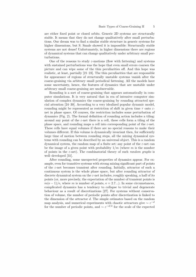
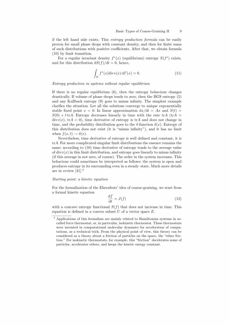
Rounding is a sort of coarse-graining that appears automatically in com-puter simulations. It is very natural that in era of intensive computer sim-ulation of complex dynamics the coarse-graining by rounding attracted spe-cial attention [24–30]. According to a very idealized popular dynamic model,rounding might be represented as restriction of shift in given time τ onto ε-net in phase space. Of courses, the restriction includes some perturbation ofdynamics (Fig. 2). The formal definition of rounding action includes a tiling:around any point of the ε-net there is a cell, these cells form a tiling of thephase space, and rounding maps a cell into corresponding point of the ε-net.These cells have equal volumes if there are no special reasons to make theirvolumes different. If this volume is dynamically invariant then, for sufficientlylarge time of motion between rounding steps, all the mixing dynamical sys-tems with rounding can be described by an universal object. This is a randomdynamical system, the random map of a finite set: any point of the ε-net canbe the image of a given point with probability 1/m (where m is the numberof points in the ε-net). The combinatorial theory of such random graphs iswell–developed [31].
After rounding, some unexpected properties of dynamics appear. For ex-ample, even for transitive systems with strong mixing significant part of pointsof the ε-net becomes transient after rounding. Initially, attractor of such acontinuous system is the whole phase space, but after rounding attractor ofdiscrete dynamical system on the ε-net includes, roughly speaking, a half of itspoints (or, more precisely, the expectation of the number of transient points ism(e − 1)/e, where m is number of points, e = 2.7...). In some circumstances,complicated dynamics has a tendency to collapse to trivial and degeneratebehaviour as a result of discretizations [27]. For systems without conserva-tion of volume, the number of periodic points after discretization is linked tothe dimension of the attractor d. The simple estimates based on the randommap analysis, and numerical experiments with chaotic attractors give ∼ ε−d
for the number of periodic points, and ∼ ε−d/2 for the scale of the expected
6 Alexander N. Gorban
a)
Rounding
Superposition“motion & rounding”
Motion
(during time )b)
Fig. 2. Motion, rounding and “motion with rounding” for a dynamical system (a),and the universal result of motion with rounding: a random dynamical system (b).
period [26, 30]. The first of them is just the number of points in ε-net in d-dimensional compact, the second becomes clear after the following remark.Let us imagine a random walk in a finite set with m elements (a ε-net). Whenthe length of the trajectory is of order
√m then the next step returns the
point to the trajectory with probability ∼ 1/√
m, and a loop appears withexpected period ∼ √
m (a half of the trajectory length). After ∼ √m steps
the probability of a loop appearance is near 1, hence, for the whole systemthe expected period is ∼ √
m ∼ ε−d/2.It is easy to demonstrate the difference between coarse-graining by fat-
tening and coarse-graining by rounding. Let us consider a trivial dynamicson a connected phase space: let the shift in time be identical transformation.For coarse-graining by fattening the ε-motion of any point tends to cover thewhole phase space for any positive ε and time t → ∞: periodical ε-fatteningwith trivial dynamics transforms, after time nτ , a point into the sum of n ε-balls. For coarse-graining by rounding this trivial dynamical system generatesthe same trivial dynamical system on ε-net: nothing moves.
Coarse-graining by small noise seems to be very natural. We add smallrandom term to the right hand side of differential equations that describedynamics. Instead of the Liouville equation for probability density the Fokker–Planck equation appears. There is no fundamental difference between varioustypes of coarse-graining, and the coarse-graining by ε-fattening includes majorresults about the coarse-graining by small noise that are insensitive to mostdetails of noise distribution. But the knowledge of noise distribution givesus additional tools. The action functional is such a tool for the descriptionof fluctuations [32]. Let Xε(t) be a random process “dynamics with ε-smallfluctuation” on the time interval [0, T ]. It is possible to introduce such afunctional S[ϕ] on functions x = ϕ(t) (t ∈ [0, T ]) that for sufficiently smallε, δ > 0
P‖Xε − ϕ‖ < δ ≈ exp(−S[ϕ]/ε2).
Basic Types of Coarse-Graining II 7
Action functional is constructed for various types of random perturbations[32]. Introduction to the general theory of random dynamical systems withinvariant measure is presented in [33].
In following sections, we consider two types of coarse-graining: the Ehren-fests’ coarse-graining and its extension to a general principle of non-equilibriumthermodynamics, and the coarse-graining based on the uncertainty of dynam-ical models and ε-motions.
2 The Ehrenfests’ Coarse-graining
2.1 Kinetic equation and entropy
Entropy conservation in systems with conservation of phase volume
The Erenfest’s coarse-graining was originally defined for conservative3 sys-tems. Usually, Hamiltonian systems are considered as conservative ones, butin all constructions only one property of Hamiltonian systems is used, namely,conservation of the phase volume dΓ (the Liouville theorem). Let X be phasespace, v(x) be a vector field, dΓ = dnx be the differential of phase volume.The flow,
dx
dt= v(x), (1)
conserves the phase volume, if divv(x) = 0. The continuity equation,
∂f
∂t= −
∑
i
∂(fvi(x))
∂xi, (2)
describes the induced dynamics of the probability density f(x, t) on phasespace. For incompressible flow (conservation of volume), the continuity equa-tion can be rewritten in the form
∂f
∂t= −
∑
i
vi(x)∂f
∂xi. (3)
This means that the probability density is constant along the flow: f(x, t +dt) = f(x − v(x)dt, t). Hence, for any continuous function h(f) the integral
H(f) =
∫
X
h(f(x)) dΓ (x) (4)
3 In this paper, we use the term “conservative” as an opposite term to “dissipative:”conservative = with entropy conservation. Another use of the term “conservativesystem” is connected with energy conservation. For kinetic systems under con-sideration conservation of energy is a simple linear balance, and we shall use thefirst sense only.
8 Alexander N. Gorban
does not change in time, provided the probability density satisfies the con-tinuity equation (2) and the flow v(x) conserves the phase volume. Forh(f) = −f ln f integral (4) gives the classical Boltzmann–Gibbs–Shannon(BGS) entropy functional:
S(f) = −∫
X
f(x) ln(f(x)) dΓ (x). (5)
For flows with conservation of volume, entropy is conserved: dS/dt ≡ 0 .
Kullback entropy conservation in systems with regular invariant distribution
Suppose the phase volume is not invariant with respect to flow (1), but aregular invariant density f∗(x) (equilibrium) exists:
∑
i
∂(f∗(x)vi(x))
∂xi= 0. (6)
In this case, instead of an invariant phase volume dΓ , we have an invariantvolume f∗(x) dΓ . We can use (6) instead of the incompressibility conditionand rewrite (2):
∂(f(x, t)/f∗(x))
∂t= −
∑
i
vi(x)∂(f(x, t)/f∗(x))
∂xi. (7)
The function f(x, t)/f∗(x) is constant along the flow, the measure f∗(x) dΓ (x)is invariant, hence, for any continuous function h(f) integral
H(f) =
∫
X
h(f(x, t)/f∗(x))f∗(x) dΓ (x) (8)
does not change in time, if the probability density satisfies the continuityequation. For h(f) = −f ln f integral (8) gives the Kullback entropy functional[42]:
SK(f) = −∫
X
f(x) ln
(f(x)
f∗(x)
)dΓ (x). (9)
This situation does not differ significantly from the entropy conservation insystems with conservation of volume. It is just a kind of change of variables.
General entropy production formula
Let us consider the general case without assumptions about phase volumeinvariance and existence of a regular invariant density (6). In this case, let aprobability density f(x, t) be a solution of the continuity equation (2). Forthe BGS entropy functional (5)
dS(f)
dt=
∫
X
f(x, t)divv(x) dΓ (x), (10)
Basic Types of Coarse-Graining II 9
if the left hand side exists. This entropy production formula can be easilyproven for small phase drops with constant density, and then for finite sumsof such distributions with positive coefficients. After that, we obtain formula(10) by limit transition.
For a regular invariant density f∗(x) (equilibrium) entropy S(f∗) exists,and for this distribution dS(f)/dt = 0, hence,
∫
X
f∗(x)divv(x) dΓ (x) = 0. (11)
Entropy production in systems without regular equilibrium
If there is no regular equilibrium (6), then the entropy behaviour changesdrastically. If volume of phase drops tends to zero, then the BGS entropy (5)and any Kullback entropy (9) goes to minus infinity. The simplest exampleclarifies the situation. Let all the solutions converge to unique exponentiallystable fixed point x = 0. In linear approximation dx/dt = Ax and S(t) =S(0) + t trA. Entropy decreases linearly in time with the rate trA (trA =divv(x), trA < 0), time derivative of entropy is trA and does not change intime, and the probability distribution goes to the δ-function δ(x). Entropy ofthis distribution does not exist (it is “minus infinity”), and it has no limitwhen f(x, t) → δ(x).
Nevertheless, time derivative of entropy is well defined and constant, it istrA. For more complicated singular limit distributions the essence remains thesame: according to (10) time derivative of entropy tends to the average valueof divv(x) in this limit distribution, and entropy goes linearly to minus infinity(if this average in not zero, of course). The order in the system increases. Thisbehaviour could sometimes be interpreted as follows: the system is open andproduces entropy in its surrounding even in a steady–state. Much more detailsare in review [41].4
Starting point: a kinetic equation
For the formalization of the Ehrenfests’ idea of coarse-graining, we start froma formal kinetic equation
df
dt= J(f) (12)
with a concave entropy functional S(f) that does not increase in time. Thisequation is defined in a convex subset U of a vector space E.
4 Applications of this formalism are mainly related to Hamiltonian systems in so-called force thermostat, or, in particular, isokinetic thermostat. These thermostatswere invented in computational molecular dynamics for acceleration of compu-tations, as a technical trick. From the physical point of view, this theory can beconsidered as a theory about a friction of particles on the space, the “ether fric-tion.” For isokinetic thermostats, for example, this “friction” decelerates some ofparticles, accelerates others, and keeps the kinetic energy constant.
10 Alexander N. Gorban
Let us specify some notations: ET is the adjoint to the E space. Adjointspaces and operators will be indicated by T , whereas the notation ∗ is ear-marked for equilibria and quasi-equilibria.
We recall that, for an operator A : E1 → E2, the adjoint operator, AT :ET
1 → ET2 is defined by the following relation: for any l ∈ ET
2 and ϕ ∈ E1,l(Aϕ) = (AT l)(ϕ).
Next, DfS(f) ∈ ET is the differential of the functional S(f), D2fS(f)
is the second differential of the functional S(f). The quadratic functionalD2
fS(f)(ϕ,ϕ) on E is defined by the Taylor formula,
S(f + ϕ) = S(f) + DfS(f)(ϕ) +1
2D2
fS(f)(ϕ,ϕ) + o(‖ϕ‖2). (13)
We keep the same notation for the corresponding symmetric bilinear form,D2
fS(f)(ϕ,ψ), and also for the linear operator, D2fS(f) : E → ET , defined by
the formula (D2fS(f)ϕ)(ψ) = D2
fS(f)(ϕ,ψ). In this formula, on the left hand
side D2fS(f) is the operator, on the right hand side it is the bilinear form.
Operator D2fS(f) is symmetric on E, D2
fS(f)T = D2fS(f).
In finite dimensions the functional DfS(f) can be presented simply as arow vector of partial derivatives of S, and the operator D2
fS(f) is a matrixof second partial derivatives. For infinite–dimensional spaces some complica-tions exist because S(f) is defined only for classical densities and not for alldistributions. In this paper we do not pay attention to these details.
We assume strict concavity of S, D2fS(f)(ϕ,ϕ) < 0 if ϕ 6= 0. This means
that for any f the positive definite quadratic form −D2fS(f)(ϕ,ϕ) defines a
scalar product〈ϕ,ψ〉f = −(D2
fS)(ϕ,ψ). (14)
This entropic scalar product is an important part of thermodynamic formal-ism. For the BGS entropy (5) as well as for the Kullback entropy (9)
〈ϕ,ψ〉f =
∫ϕ(x)ψ(x)
f(x)dx. (15)
The most important assumption about kinetic equation (12) is: entropydoes not decrease in time:
dS
dt= (DfS(f))(J(f)) ≥ 0. (16)
A particular case of this assumption is: the system (12) is conservative andentropy is constant. The main example of such conservative equations is theLiouville equation with linear vector field J(f) = −Lf = H, f, where H, fis the Poisson bracket with Hamiltonian H.
For the following consideration of the Ehrenfests’ coarse-graining the un-derlying mechanical motion is not crucial, and it is possible to start from theformal kinetic equation (12) without any mechanical interpretation of vec-tors f . We develop below the coarse-graining procedure for general kinetic
Basic Types of Coarse-Graining II 11
equation (12) with non-decreasing entropy (16). After coarse-graining the en-tropy production increases: conservative systems become dissipative ones, anddissipative systems become “more dissipative.”
2.2 Conditional equilibrium instead of averaging in cells
Microdescription, macrodescription and quasi-equilibrium state
Averaging in cells is a particular case of entropy maximization. Let the phasespace be divided into cells. For the ith cell the population Mi is
Mi = mi(f) =
∫
celli
f(x) dΓ (x).
The averaging in cells for a given vector of populations M = (Mi) producesthe solution of the optimization problem for the BGS entropy:
S(f) → max, m(f) = M, (17)
where m(f) is vector (mi(f)). The maximizer is a function f∗M (x) defined by
the vector of averages M .This operation has a well-known generalization. In the more general state-
ment, vector f is a microscopic description of the system, vector M gives amacroscopic description, and a linear operator m transforms a microscopicdescription into a macroscopic one: M = m(f). The standard example isthe transformation of the microscopic density into the hydrodynamic fields(density–velocity–kinetic temperature) with local Maxwellian distributions asentropy maximizers (see, for example, [4]).
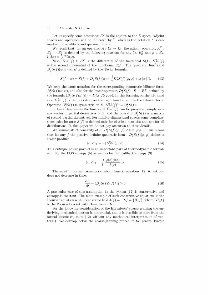
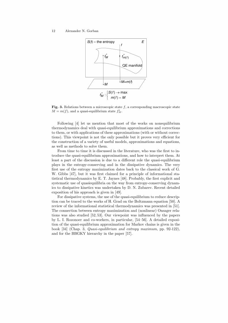
For any macroscopic description M , let us define the correspondent f∗M as a
solution to optimization problem (17) with an appropriate entropy functionalS(f) (Fig. 3). This f∗
M has many names in the literature: MaxEnt distribu-tion, reference distribution (reference of the macroscopic description to themicroscopic one), generalized canonical ensemble, conditional equilibrium, orquasi-equilibrium. We shall use here the last term.
The quasi-equilibrium distribution f∗M satisfies the obvious, but important
identity of self-consistency:m(f∗
M ) = M, (18)
or in differential form
m(DMf∗M ) = 1, i.e. m((DMf∗
M )a) ≡ a. (19)
The last identity means that the infinitesimal change in M calculated throughdifferential of the quasi-equilibrium distribution f∗
M is simply the infinitesimalchange in M . For the second differential we obtain
m(D2Mf∗
M ) = 0, i.e. m((D2Mf∗
M )(a, b)) ≡ 0. (20)
12 Alexander N. Gorban
QE manifold
S(f) – the entropy E
M
*Mf
M=m(f)
f
*)(fmf
Mfm
fSfM
)(
max)(:*
Fig. 3. Relations between a microscopic state f , a corresponding macroscopic stateM = m(f), and a quasi-equilibrium state f∗
M .
Following [4] let us mention that most of the works on nonequilibriumthermodynamics deal with quasi-equilibrium approximations and correctionsto them, or with applications of these approximations (with or without correc-tions). This viewpoint is not the only possible but it proves very efficient forthe construction of a variety of useful models, approximations and equations,as well as methods to solve them.
From time to time it is discussed in the literature, who was the first to in-troduce the quasi-equilibrium approximations, and how to interpret them. Atleast a part of the discussion is due to a different role the quasi-equilibriumplays in the entropy-conserving and in the dissipative dynamics. The veryfirst use of the entropy maximization dates back to the classical work of G.W. Gibbs [47], but it was first claimed for a principle of informational sta-tistical thermodynamics by E. T. Jaynes [48]. Probably, the first explicit andsystematic use of quasiequilibria on the way from entropy-conserving dynam-ics to dissipative kinetics was undertaken by D. N. Zubarev. Recent detailedexposition of his approach is given in [49].
For dissipative systems, the use of the quasi-equilibrium to reduce descrip-tion can be traced to the works of H. Grad on the Boltzmann equation [50]. Areview of the informational statistical thermodynamics was presented in [51].The connection between entropy maximization and (nonlinear) Onsager rela-tions was also studied [52, 53]. Our viewpoint was influenced by the papersby L. I. Rozonoer and co-workers, in particular, [54–56]. A detailed exposi-tion of the quasi-equilibrium approximation for Markov chains is given in thebook [34] (Chap. 3, Quasi-equilibrium and entropy maximum, pp. 92-122),and for the BBGKY hierarchy in the paper [57].
Basic Types of Coarse-Graining II 13
The maximum entropy principle was applied to the description of theuniversal dependence of the three-particle distribution function F3 on the two-particle distribution function F2 in classical systems with binary interactions[58]. For a discussion of the quasi-equilibrium moment closure hierarchies forthe Boltzmann equation [55] see the papers [59–61]. A very general discussionof the maximum entropy principle with applications to dissipative kinetics isgiven in the review [62]. Recently, the quasi-equilibrium approximation withsome further correction was applied to the description of rheology of polymersolutions [64,65] and of ferrofluids [66,67]. Quasi-equilibrium approximationsfor quantum systems in the Wigner representation [70,71] was discussed veryrecently [63].
We shall now introduce the quasi-equilibrium approximation in the mostgeneral setting. The coarse-graining procedure will be developed after that asa method for enhancement of the quasi-equilibrium approximation [5].
Quasi-equilibrium manifold, projector and approximation
A quasi-equilibrium manifold is a set of quasi-equilibrium states f∗M parame-
terized by macroscopic variables M . For microscopic states f the correspon-dent quasi-equilibrium states are defined as f∗
m(f). Relations between f , M ,f∗
M , and f∗m(f) are presented in Fig. 3.
A quasi-equilibrium approximation for the kinetic equation (12) is an equa-tion for M(t):
dM
dt= m(J(f∗
M )). (21)
To define M in the quasi-equilibrium approximation for given M , we find thecorrespondent quasi-equilibrium state f∗
M and the time derivative of f in thisstate J(f∗
M ), and then return to the macroscopic variables by the operator m.If M(t) satisfies (21) then f∗
M(t) satisfies the following equation
df∗M
dt= (DMf∗
M )
(dM
dt
)= (DMf∗
M )(m(J(f∗M ))). (22)
The right hand side of (22) is the projection of vector field J(f) onto thetangent space of the quasi-equilibrium manifold at the point f = f∗
M . Aftercalculating the differential DMf∗
M from the definition of quasi-equilibrium(17), we obtain df∗
M/dt = πf∗M
J(f∗M ), where πf∗
Mis the quasi-equilibrium
projector:
πf∗M
= (DMf∗M )m =
(D2
fS)−1
f∗M
mT(m
(D2
fS)−1
f∗M
mT)−1
m. (23)
It is straightforward to check the equality π2f∗
M= πf∗
M, and the self-adjointness
of πf∗M
with respect to entropic scalar product (14). In this scalar product,the quasi-equilibrium projector is the orthogonal projector onto the tangentspace to the quasi-equilibrium manifold. The quasi-equilibrium projector for
14 Alexander N. Gorban
– QE manifold
E
M
*Mf
*Mf
T
J
)(* JMf
*Mf
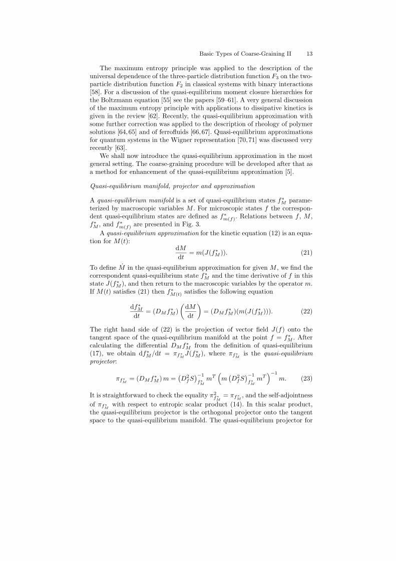
Fig. 4. Quasi-equilibrium manifold Ω, tangent space Tf∗M
Ω, quasi-equilibrium pro-jector πf∗
M, and defect of invariance, ∆f∗
M= J − πf∗
M(J).
a quasi-equilibrium approximation was first constructed by B. Robertson [68].Thus, we have introduced the basic constructions: quasi-equilibrium man-
ifold, entropic scalar product, and quasi-equilibrium projector (Fig. 4).
Preservation of dissipation
For the quasi-equilibrium approximation the entropy is S(M) = S(f∗M ). For
this entropy,dS(M)
dt=
(dS(f)
dt
)
f=f∗M
, (24)
Here, on the left hand side stands the macroscopic entropy production for thequasi-equilibrium approximation (21), and the right hand side is the micro-scopic entropy production calculated for the initial kinetic equation (12). Thisequality implies preservation of the type of dynamics [34, 35]:
• If for the initial kinetics (12) the dissipativity inequality (16) holds thenthe same inequality is true for the quasi-equilibrium approximation (21);
• If the initial kinetics (12) is conservative then the quasi-equilibrium ap-proximation (21) is conservative also.
For example, let the initial kinetic equation be the Liouville equation for asystem of many identical particles with binary interaction. If we choose asmacroscopic variables the one-particle distribution function, then the quasi-equilibrium approximation is the Vlasov equation. If we choose as macroscopicvariables the hydrodynamic fields, then the quasi-equilibrium approximationis the compressible Euler equation with self–interaction of liquid. Both of theseequations are conservative and turn out to be even Hamiltonian systems [69].
Basic Types of Coarse-Graining II 15
Measurement of accuracy
Accuracy of the quasi-equilibrium approximation near a given M can be mea-sured by the defect of invariance (Fig. 4):
∆f∗M
= J(f∗M ) − πf∗
MJ(f∗
M ). (25)
A dimensionless criterion of accuracy is the ratio ‖∆f∗M‖/‖J(f∗
M )‖ (a “sine”of the angle between J and tangent space). If ∆f∗
M≡ 0 then the quasi-
equilibrium manifold is an invariant manifold, and the quasi-equilibrium ap-proximation is exact. In applications, the quasi-equilibrium approximation isusually not exact.
The Gibbs entropy and the Boltzmann entropy
For analysis of micro-macro relations some authors [77, 78] call entropy S(f)the Gibbs entropy, and introduce a notion of the Boltzmann entropy. Boltz-mann defined the entropy of a macroscopic system in a macrostate M as thelog of the volume of phase space (number of microstates) corresponding toM . In the proposed level of generality [34, 35], the Boltzmann entropy of thestate f can be defined as SB(f) = S(f∗
m(f)). It is entropy of the projection of f
onto quasi-equilibrium manifold (the “shadow” entropy). For conservative sys-tems the Gibbs entropy is constant, but the Boltzmann entropy increases [35](during some time, at least) for motions that start on the quasi-equilibriummanifold, but not belong to this manifold.
These notions of the Gibbs or Boltzmann entropy are related to micro-macro transition and may be applied to any convex entropy functional, notthe BGS entropy (5) only. This may cause some terminological problems (wehope, not here), and it may be better just to call S(f∗
m(f)) the macroscopicentropy.
Invariance equation and the Chapman–Enskog expansion
The first method for improvement of the quasi-equilibrium approximationwas the Chapman–Enskog method for the Boltzmann equation [79]. It usesthe explicit structure of singularly perturbed systems. Many other methodswere invented later, and not all of them use this explicit structure (see, forexample review in [4]). Here we develop the Chapman–Enskog method forone important class of model equations that were invented to substitute theBoltzmann equation and other more complicated systems when we don’t knowthe details of microscopic kinetics. It includes the well-known Bhatnagar–Gross–Krook (BGK) kinetic equation [38] , as well as wide class of generalizedmodel equations [39].
As a starting point we take a formal kinetic equation with a small param-eter ǫ
df
dt= J(f) = F (f) +
1
ǫ(f∗
m(f) − f). (26)
16 Alexander N. Gorban
The term (f∗m(f) − f) is non-linear because nonlinear dependency f∗
m(f) on
m(f).We would like to find a reduced description valid for macroscopic vari-
ables M . It means, at least, that we are looking for an invariant manifoldparameterized by M , f = fM , that satisfies the invariance equation:
(DMfM )(m(J(fM ))) = J(fM ). (27)
The invariance equation means that the time derivative of f calculatedthrough the time derivative of M (M = m(J(fM ))) by the chain rule co-incides with the true time derivative J(f). This is the central equation for themodel reduction theory and applications. First general results about existenceand regularity of solutions to that equation were obtained by Lyapunov [83](see review in [3, 4]). For kinetic equation (26) the invariance equation has aform
(DMfM )(m(F (fM ))) = F (fM ) +1
ǫ(f∗
M − fM ), (28)
because the self-consistency identity (18).Due to presence of small parameter ǫ in J(f), the zero approximation is
obviously the quasi-equilibrium approximation: f(0)M = f∗
M . Let us look for fM
in the form of power series: fM = f(0)M + ǫf
(1)M + . . .; m(f
(k)M ) = 0 for k ≥ 1.
From (28) we immediately find:
f(1)M = F (f
(0)M ) − (DMf
(0)M )(m(F (f
(0)M ))) = ∆f∗
M. (29)
It is very natural that the first term of the Chapman–Enskog expansion formodel equations (26) is just the defect of invariance for the quasi-equilibriumapproximation. Calculation of the following terms is also straightforward.
The correspondent first–order in ǫ approximation for the macroscopicequations is:
dM
dt= m(F (f∗
M )) + ǫm((DfF (f))f∗M
∆f∗M
). (30)
We should remind that m(∆f∗M
) = 0. The last term in (28) vanishes in macro-scopic projection for all orders.
The typical situation for the model equations (26) is: the vector field F (f)is conservative, (DfS(f))F (f) = 0. In that case, the first term m(F (f∗
M )) alsoconserves the correspondent Boltzmann (i.e. macroscopic, but not obligatoryBGS) entropy S(f∗
M ). But the straightforward calculation of the Boltzmannentropy S(f∗
M ) production for the first-order Chapman–Enskog term in equa-tion (30) gives us for conservative F (f):
dS(M)
dt= ǫ〈∆f∗
M,∆f∗
M〉f∗
M≥ 0. (31)
where 〈•, •〉f is the entropic scalar product (14). The Boltzmann entropyproduction in the first Chapman–Enskog approximation is zero if and only if∆f∗
M= 0, i.e. if at point M the quasi-equilibrium manifold is locally invariant.
Basic Types of Coarse-Graining II 17
M
dM/dt=F(M) ??? Macroscopic equation
The chain
df/dt=J(f) QE manifold
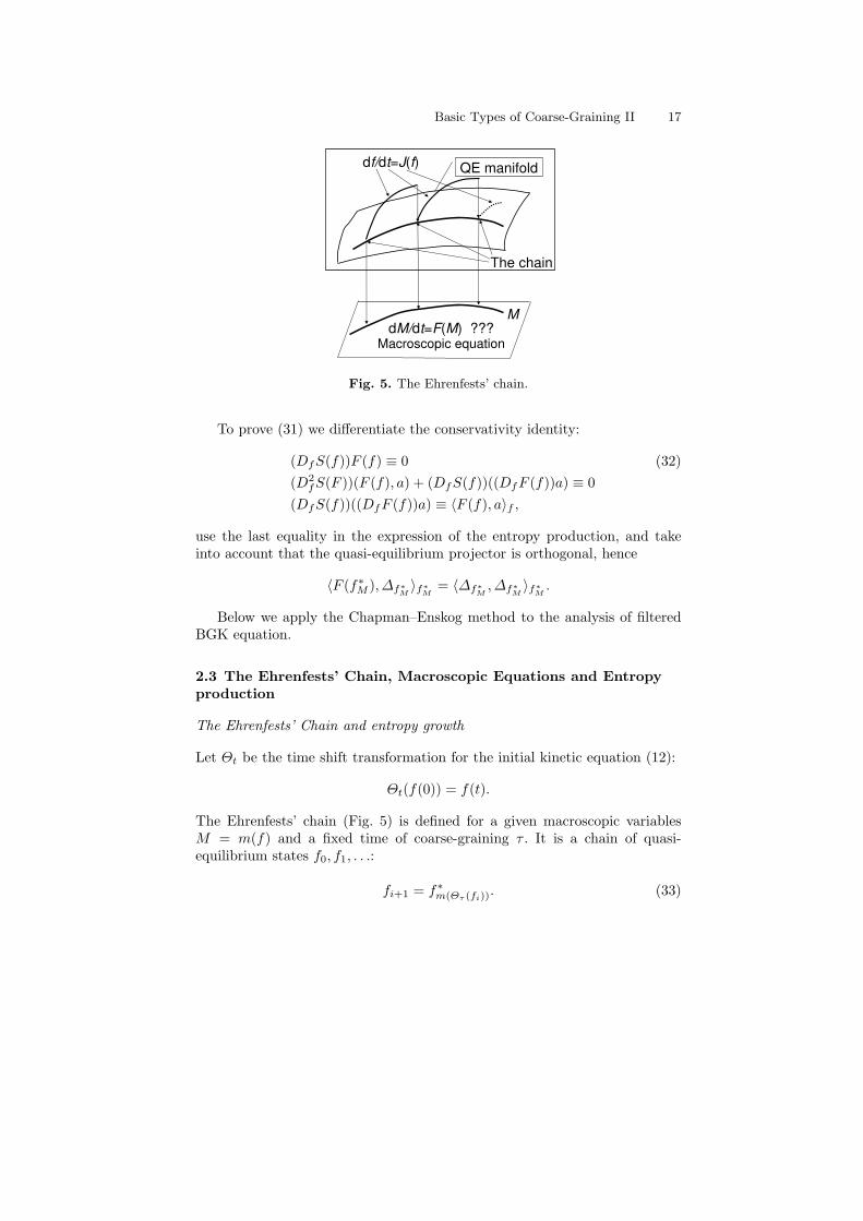
Fig. 5. The Ehrenfests’ chain.
To prove (31) we differentiate the conservativity identity:
(DfS(f))F (f) ≡ 0 (32)
(D2fS(F ))(F (f), a) + (DfS(f))((DfF (f))a) ≡ 0
(DfS(f))((DfF (f))a) ≡ 〈F (f), a〉f ,
use the last equality in the expression of the entropy production, and takeinto account that the quasi-equilibrium projector is orthogonal, hence
〈F (f∗M ),∆f∗
M〉f∗
M= 〈∆f∗
M,∆f∗
M〉f∗
M.
Below we apply the Chapman–Enskog method to the analysis of filteredBGK equation.
2.3 The Ehrenfests’ Chain, Macroscopic Equations and Entropy
production
The Ehrenfests’ Chain and entropy growth
Let Θt be the time shift transformation for the initial kinetic equation (12):
Θt(f(0)) = f(t).
The Ehrenfests’ chain (Fig. 5) is defined for a given macroscopic variablesM = m(f) and a fixed time of coarse-graining τ . It is a chain of quasi-equilibrium states f0, f1, . . .:
fi+1 = f∗m(Θτ (fi))
. (33)
18 Alexander N. Gorban
To get the next point of the chain, fi+1, we take fi, move it by the time shiftΘτ , calculate the corresponding macroscopic state Mi+1 = m(Θτ (fi)), andfind the quasi-equilibrium state f∗
Mi+1= fi+1.
If the point Θτ (fi) is not a quasi-equilibrium state, then S(Θτ (fi)) <S(f∗
m(Θτ (fi))) because of quasi-equilibrium definition (17) and strict concavity
of entropy. Hence, if the motion between fi and Θτ (fi) does not belong tothe quasi-equilibrium manifold, then S(fi+1) > S(fi), entropy in the Ehren-fests’ chain grows. The entropy gain consists of two parts: the gain in themotion (from fi to Θτ (fi)), and the gain in the projection (from Θτ (fi) tofi+1 = f∗
m(Θτ (fi))). Both parts are non-negative. For conservative systems the
first part is zero. The second part is strictly positive if the motion leavesthe quasi-equilibrium manifold. Hence, we observe some sort of duality be-tween entropy production in the Ehrenfests’ chain and invariance of the quasi-equilibrium manifold. The motions that build the Ehrenfests’ chain restart pe-riodically from the quasi-equilibrium manifold and the entropy growth alongthis chain is similar to the Boltzmann entropy growth in the Chapman–Enskogapproximation, and that similarity is very deep, as the exact formulas showbelow.
The natural projector and macroscopic dynamics
How to use the Ehrenfests’ chains? First of all, we can try to define the macro-scopic kinetic equations for M(t) by the requirement that for any initial pointof the chain f0 the solution of these macroscopic equations with initial con-ditions M(0) = m(f0) goes through all the points m(fi): M(nτ) = m(fn)(n = 1, 2, . . .) (Fig. 5) [5] (see also [4]). Another way is an “equation–freeapproach” [9] to the direct computation of the Ehrenfests’ chain with a com-bination of microscopic simulation and macroscopic stepping.
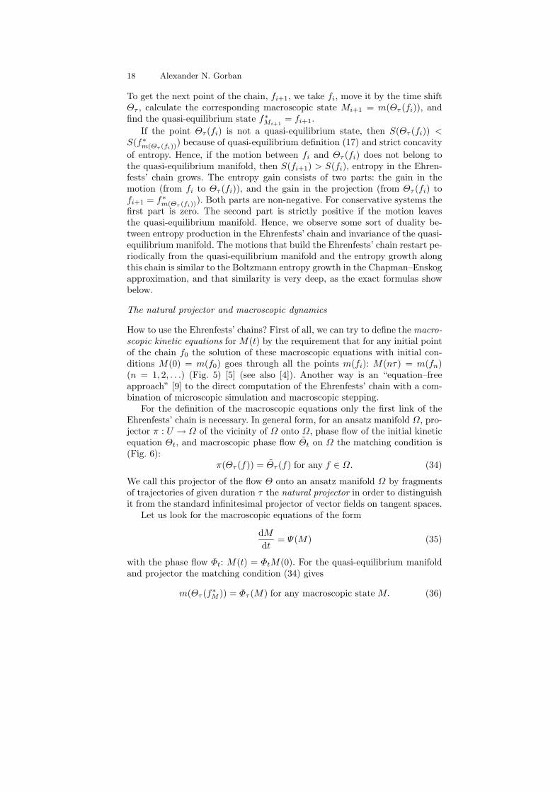
For the definition of the macroscopic equations only the first link of theEhrenfests’ chain is necessary. In general form, for an ansatz manifold Ω, pro-jector π : U → Ω of the vicinity of Ω onto Ω, phase flow of the initial kineticequation Θt, and macroscopic phase flow Θt on Ω the matching condition is(Fig. 6):
π(Θτ (f)) = Θτ (f) for any f ∈ Ω. (34)
We call this projector of the flow Θ onto an ansatz manifold Ω by fragmentsof trajectories of given duration τ the natural projector in order to distinguishit from the standard infinitesimal projector of vector fields on tangent spaces.
Let us look for the macroscopic equations of the form
dM
dt= Ψ(M) (35)
with the phase flow Φt: M(t) = ΦtM(0). For the quasi-equilibrium manifoldand projector the matching condition (34) gives
m(Θτ (f∗M )) = Φτ (M) for any macroscopic state M. (36)
Basic Types of Coarse-Graining II 19
Fig. 6. Projection of segments of trajectories: The microscopic motion above themanifold Ω and the macroscopic motion on this manifold. If these motions beginin the same point on Ω, then, after time τ , projection of the microscopic stateonto Ω should coincide with the result of the macroscopic motion on Ω. For quasi-equilibrium Ω, projector π : E → Ω acts as π(f) = f∗
m(f).
This condition is the equation for the macroscopic vector field Ψ(M). Thesolution of this equation is a function of τ : Ψ = Ψ(M, τ). For sufficientlysmooth microscopic vector field J(f) and entropy S(f) it is easy to find theTaylor expansion of Ψ(M, τ) in powers of τ . It is a straightforward exercisein differential calculus. Let us find the first two terms: Ψ(M, τ) = Ψ0(M) +τΨ1(M) + o(τ). Up to the second order in τ the matching condition (36) is
m(J(f∗M ))τ + m((DfJ(f))f=f∗
M(J(f∗
M )))τ2
2
= Ψ0(M)τ + Ψ1(M)τ2 + (DMΨ0(M))(Ψ0(M))τ2
2. (37)
From this condition immediately follows:
Ψ0(M) = m(J(f∗M )); (38)
Ψ1(M) =1
2m[(DfJ(f))f=f∗
M(J(f∗
M )) − (DMJ(f∗M ))(m(J(f∗
M )))]
= m((DfJ(f))f=f∗M
∆f∗M
)
where ∆f∗M
is the defect of invariance (25). The macroscopic equation in thefirst approximation is:
20 Alexander N. Gorban
dM
dt= m(J(f∗
M )) +τ
2m((DfJ(f))f=f∗
M∆f∗
M). (39)
It is exactly the first Chapman–Enskog approximation (30) for the model ki-netics (26) with ε = τ/2. The first term m(J(f∗
M )) gives the quasi-equilibriumapproximation, the second term increases dissipation. The formula for entropyproduction follows from (39) [11]. If the initial microscopic kinetic (12) is con-servative, then for macroscopic equation (39) we obtain as for the Chapman–Enskog approximation:
dS(M)
dt=
τ
2〈∆f∗
M,∆f∗
M〉f∗
M, (40)
where 〈•, •〉f is the entropic scalar product (14). From this formula we seeagain a duality between the invariance of the quasi-equilibrium manifold andthe dissipativity: entropy production is proportional to the square of the defectof invariance of the quasi-equilibrium manifold.
For linear microscopic equations (J(f) = Lf) the form of the macroscopicequations is
dM
dt= mL
[1 +
τ
2(1 − πf∗
M)L
]f∗
M , (41)
where πf∗M
is the quasi-equilibrium projector (23).
The Navier–Stokes equation from the free flight dynamics
The free flight equation describes dynamics of one-particle distribution func-tion f(x,v) due to free flight:
∂f(x,v, t)
∂t= −
∑
i
vi∂f(x,v, t)
∂xi. (42)
The difference from the continuity equation (2) is that there is no velocityfield v(x), but the velocity vector v is an independent variable. Equation (42)is conservative and has an explicit general solution
f(x,v, t) = f0(x − vt,v). (43)
The coarse-graining procedure for (42) serves for modeling kinetics with anunknown dissipative term I(f)
∂f(x,v, t)
∂t= −
∑
i
vi∂f(x,v, t)
∂xi+ I(f). (44)
The Ehrenfests’ chain realizes a splitting method for (44): first, the free flightstep during time τ , than the complete relaxation to a quasi-equilibrium dis-tribution due to dissipative term I(f), then again the free flight, and so on.In this approximation the specific form of I(f) is not in use, and the only
Basic Types of Coarse-Graining II 21
parameter is time τ . It is important that this hypothetical I(f) preservesall the standard conservation laws (number of particles, momentum, and en-ergy) and has no additional conservation laws: everything else relaxes. Fol-lowing this assumption, the macroscopic variables are: M0 = n(x, t) =
∫fdv,
Mi = nui =∫
vifdv (i = 1, 2, 3), M4 = 3nkBTm + nu2 =
∫v2fdv. The zero-
order (quasi-equilibrium) approximation (21) gives the classical Euler equa-tion for compressible non-isothermal gas. In the first approximation (39) weobtain the Navier–Stokes equations:
∂n
∂t= −
∑
i
∂(nui)
∂xi,
∂(nuk)
∂t= −
∑
i
∂(nukui)
∂xi− 1
m
∂P
∂xk
+τ
2
1
m
∑
i
∂
∂xi
[P
(∂uk
∂xi+
∂ui
∂xk− 2
3δkidivu
)], (45)
∂E∂t
= −∑
i
∂(Eui)
∂xi− 1
m
∑
i
∂(Pui)
∂xi+
τ
2
5kB
2m2
∑
i
∂
∂xi
(P
∂T
∂xi
),
where P = nkBT is the ideal gas pressure, E = 12
∫v2f dv = 3nkBT
2m + n2 u2 is
the energy density per unite mass (P = 2m3 E − mn
3 u2, T = 2m3nkB
E − m3kB
u2),and the underlined terms are results of the coarse-graining additional to thequasi-equilibrium approximation.
The dynamic viscosity in (45) is µ = τ2nkBT . It is useful to compare this
formula to the mean–free–path theory that gives µ = τcolnkBT = τcolP , whereτcol is the collision time (the time for the mean–free–path). According to theseformulas, we get the following interpretation of the coarse-graining time τ forthis example: τ = 2τcol.
The equations obtained (45) coincide with the first–order terms of theChapman–Enskog expansion (30) applied to the BGK equations with τcol =τ/2 and meet the same problem: the Prandtl number (i.e., the dimensionlessratio of viscosity and thermal conductivity) is Pr = 1 instead of the valuePr = 2
3 verified by experiments with perfect gases and by more detailed theory[80] (recent discussion of this problem for the BGK equation with some waysfor its solution is presented in [81]).
In the next order in τ we obtain the stable post–Navier–Stokes equa-tions instead of the unstable Burnett equations that appear in the Chapman–Enskog expansion [11, 76]. Here we can see the difference between two ap-proaches.
Persistence of invariance and mistake of differential pursuit
L.M. Lewis called a generalization of the Ehernfest’s approach a “unifyingprinciple in statistical mechanics,” but he created other macroscopic equa-tions: he produced the differential pursuit (Fig. 7a)
22 Alexander N. Gorban
a)
M
dM/dt=(m(f( ))-M)/ Differential pursuit
df/dt=J(f)QE manifold
m(f( ))M=m(f(0))
b)
M
df/dt=J(f)
Invariant QE manifold
True motion
Differential pursuit
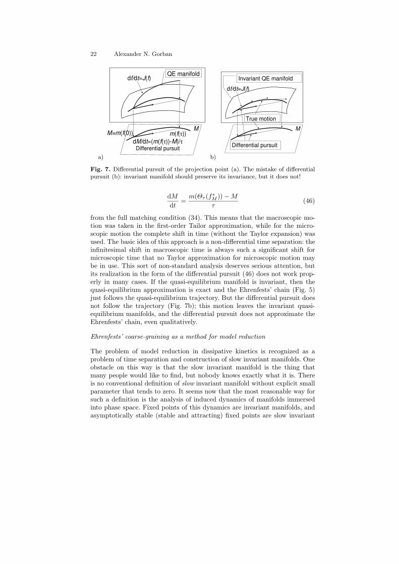
Fig. 7. Differential pursuit of the projection point (a). The mistake of differentialpursuit (b): invariant manifold should preserve its invariance, but it does not!
dM
dt=
m(Θτ (f∗M )) − M
τ(46)
from the full matching condition (34). This means that the macroscopic mo-tion was taken in the first-order Tailor approximation, while for the micro-scopic motion the complete shift in time (without the Taylor expansion) wasused. The basic idea of this approach is a non-differential time separation: theinfinitesimal shift in macroscopic time is always such a significant shift formicroscopic time that no Taylor approximation for microscopic motion maybe in use. This sort of non-standard analysis deserves serious attention, butits realization in the form of the differential pursuit (46) does not work prop-erly in many cases. If the quasi-equilibrium manifold is invariant, then thequasi-equilibrium approximation is exact and the Ehrenfests’ chain (Fig. 5)just follows the quasi-equilibrium trajectory. But the differential pursuit doesnot follow the trajectory (Fig. 7b); this motion leaves the invariant quasi-equilibrium manifolds, and the differential pursuit does not approximate theEhrenfests’ chain, even qualitatively.
Ehrenfests’ coarse-graining as a method for model reduction
The problem of model reduction in dissipative kinetics is recognized as aproblem of time separation and construction of slow invariant manifolds. Oneobstacle on this way is that the slow invariant manifold is the thing thatmany people would like to find, but nobody knows exactly what it is. Thereis no conventional definition of slow invariant manifold without explicit smallparameter that tends to zero. It seems now that the most reasonable way forsuch a definition is the analysis of induced dynamics of manifolds immersedinto phase space. Fixed points of this dynamics are invariant manifolds, andasymptotically stable (stable and attracting) fixed points are slow invariant
Basic Types of Coarse-Graining II 23
Initial ansatz manifold
Hypothetic attractive invariant manifold
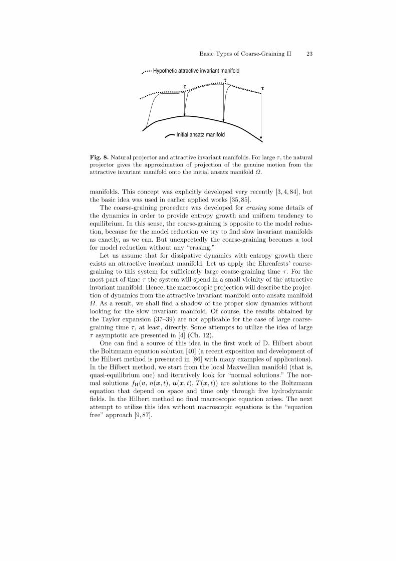
Fig. 8. Natural projector and attractive invariant manifolds. For large τ , the naturalprojector gives the approximation of projection of the genuine motion from theattractive invariant manifold onto the initial ansatz manifold Ω.
manifolds. This concept was explicitly developed very recently [3, 4, 84], butthe basic idea was used in earlier applied works [35,85].
The coarse-graining procedure was developed for erasing some details ofthe dynamics in order to provide entropy growth and uniform tendency toequilibrium. In this sense, the coarse-graining is opposite to the model reduc-tion, because for the model reduction we try to find slow invariant manifoldsas exactly, as we can. But unexpectedly the coarse-graining becomes a toolfor model reduction without any “erasing.”
Let us assume that for dissipative dynamics with entropy growth thereexists an attractive invariant manifold. Let us apply the Ehrenfests’ coarse-graining to this system for sufficiently large coarse-graining time τ . For themost part of time τ the system will spend in a small vicinity of the attractiveinvariant manifold. Hence, the macroscopic projection will describe the projec-tion of dynamics from the attractive invariant manifold onto ansatz manifoldΩ. As a result, we shall find a shadow of the proper slow dynamics withoutlooking for the slow invariant manifold. Of course, the results obtained bythe Taylor expansion (37–39) are not applicable for the case of large coarse-graining time τ , at least, directly. Some attempts to utilize the idea of largeτ asymptotic are presented in [4] (Ch. 12).
One can find a source of this idea in the first work of D. Hilbert aboutthe Boltzmann equation solution [40] (a recent exposition and development ofthe Hilbert method is presented in [86] with many examples of applications).In the Hilbert method, we start from the local Maxwellian manifold (that is,quasi-equilibrium one) and iteratively look for “normal solutions.” The nor-mal solutions fH(v, n(x, t), u(x, t), T (x, t)) are solutions to the Boltzmannequation that depend on space and time only through five hydrodynamicfields. In the Hilbert method no final macroscopic equation arises. The nextattempt to utilize this idea without macroscopic equations is the “equationfree” approach [9, 87].
24 Alexander N. Gorban
The Ehrenfests’ coarse-graining as a tool for extraction of exact macro-scopic dynamics was tested on exactly solvable problems [73]. It gives also anew approach to the fluctuation–dissipation theorems [72].
2.4 Kinetic models, entropic involution, and the second–order
“Euler method”
Time-step – dissipation decoupling problem
Sometimes, the kinetic equation is much simpler than the coarse-grained dy-namics. For example, the free flight kinetics (42) has the obvious exact ana-lytical solution (43), but the Euler or the Navier–Stokes equations (45) seemto be very far from being exactly solvable. In this sense, the Ehrenfests’ chain(33) (Fig. 5) gives a stepwise approximation to a solution of the coarse-grained(macroscopic) equations by the chain of solutions of the kinetic equations.
If we use the second-order approximation in the coarse-graining proce-dure (37), then the Ehrenfests’ chain with step τ is the second–order (intime step τ) approximation to the solution of macroscopic equation (39). Itis very attractive for hydrodynamics: the second–order in time method withapproximation just by broken line built from intervals of simple free–flightsolutions. But if we use the Ehrenfests’ chain for approximate solution, thenthe strong connection between the time step τ and the coefficient in equations(39) (see also the entropy production formula (40)) is strange. Rate of dissipa-tion is proportional to τ , and it seems to be too restrictive for computationalapplications: decoupling of time step and dissipation rate is necessary. Thisdecoupling problem leads us to a question that is strange from the Ehrenfests’coarse-graining point of view: how to construct an analogue to the Ehrenfests’coarse-graining chain, but without dissipation? The entropic involution is atool for this construction.
Entropic involution
The entropic involution was invented for improvement of the lattice–Boltzmannmethod [89]. We need to construct a chain with zero macroscopic entropy pro-duction and second order of accuracy in time step τ . The chain consists ofintervals of solution of kinetic equation (12) that is conservative. The timeshift for this equation is Θt. The macroscopic variables M = m(f) are cho-sen, and the time shift for corresponding quasi-equilibrium equation is (in
this section) Θt. The standard example is: the free flight kinetics (42,43) asa microscopic conservative kinetics, hydrodynamic fields (density–velocity–kinetic temperature) as macroscopic variables, and the Euler equations as amacroscopic quasi-equilibrium equations for conservative case (see (45), notunderlined terms).
Let us start from construction of one link of a chain and take a pointf1/2 on the quasi-equilibrium manifold. (It is not an initial point of the link,
Basic Types of Coarse-Graining II 25
f0, but a “middle” one.) The correspondent value of M is M1/2 = m(f1/2).Let us define M0 = m(Θ−τ/2(f1/2)), M1 = m(Θτ/2(f1/2)). The dissipativeterm in macroscopic equations (39) is linear in τ , hence, there is a symme-try between forward and backward motion from any quasiequilibrium initialcondition with the second-order accuracy in the time of this motion (it be-came clear long ago [35]). Dissipative terms in the shift from M0 to M1/2
(that decrease macroscopic entropy S(M)) annihilate with dissipative termsin the shift from M1/2 to M1 (that increase macroscopic entropy S(M)). As
the result of this symmetry, M1 coincides with Θτ (M0) with the second-orderaccuracy. (It is easy to check this statement by direct calculation too.)
It is necessary to stress that the second-order accuracy is achieved on theends of the time interval only: Θτ (M0) coincides with M1 = m(Θτ (f0)) in thesecond order in τ
m(Θτ (f0)) − Θτ (M0) = o(τ2).
On the way Θt(M0) from M0 to Θτ (M0) for 0 < t < τ we can guarantee thefirst-order accuracy only (even for the middle point). It is essentially the samesituation as we had for the Ehrenfests’ chain: the second order accuracy of thematching condition (36) is postulated for the moment τ , and for 0 < t < τ theprojection of the m(Θt(f0)) follows a solution of the macroscopic equation (39)with the first order accuracy only. In that sense, the method is quite differentfrom the usual second–order methods with intermediate points, for example,from the Crank–Nicolson schemes. By the way, the middle quasi-equilibriumpoint, f1/2 appears for the initiation step only. After that, we work with theend points of links.
The link is constructed. For the initiation step, we used the middlepoint f1/2 on the quasi-equilibrium manifold. The end points of the link,f0 = Θ−τ/2(f1/2) and f1 = Θτ/2(f1/2) don’t belong to the quasi-equilibriummanifold, unless it is invariant. Where are they located? They belong a surfacethat we call a film of non-equilibrium states [4,74,75]. It is a trajectory of thequasi-equilibrium manifold due to initial microscopic kinetics. In [4,74,75] westudied mainly the positive semi-trajectory (for positive time). Here we needshifts in both directions.
A point f on the film of non-equilibrium states is naturally parameterizedby M, τ : f = qM,τ , where M = m(f) is the value of the macroscopic variables,and τ(f) is the time of shift from a quasi-equilibrium state: Θ−τ (f) is a quasi-equilibrium state. In the first order in τ ,
qM,τ = f∗M + τ∆f∗
M, (47)
and the first-order Chapman–Enskog approximation (29) for the model BGKequations is also here with τ = ǫ. (The two–times difference between kineticcoefficients for the Ehrenfests’ chain and the first-order Chapman–Enskog ap-proximation appears because for the Ehrenfests’ chain the distribution walkslinearly between qM,0 and qM,τ , and for the first-order Chapman–Enskog ap-proximation it is exactly qM,τ .)
26 Alexander N. Gorban
For each M and positive s from some interval ]0, ς[ there exist two suchτ±(M, s) (τ+(M, s) > 0, τ−(M, s) < 0) that
S(qM,τ±(M,s)) = S(M) − s. (48)
Up to the second order in τ±
s =τ2±
2〈∆f∗
M,∆f∗
M〉f∗
M+ o(τ2
±) (49)
(compare to (40)), and
τ+ = −τ− + o(τ−); |τ±| =
√s
〈∆f∗M
,∆f∗M〉f∗
M
(1 + o(1)). (50)
Equation (48) describes connection between entropy change s and time co-ordinate τ on the film of non-equilibrium states, and (49) presents the firstnon-trivial term of the Taylor expansion of (48).
The entropic involution IS is the transformation of the film of non-equilibrium states:
IS(qM,τ±) = qM,τ∓ . (51)
This involution transforms τ+ into τ−, and back. For a given macroscopicstate M , the entropic involution IS transforms the curve of non-equilibriumstates qM,τ into itself.
In the first order in τ it is just reflection qM,τ → qM,−τ . A partial lineariza-tion is also in use. For this approximation, we define nonlinear involutions ofstraight lines parameterized by α, not of curves:
I0S(f) = f∗
m(f) − α(f − f∗m(f)), α > 0, (52)
with condition of entropy conservation
S(I0S(f)) = S(f). (53)
The last condition serves as equation for α. The positive solution is unique andexists for f from some vicinity of the quasi-equilibrium manifold. It followsfrom the strong concavity of entropy. The transformation I0
S (53) is definednot only on the film of non-equilibrium states, but on all distributions (mi-croscopic) f that are sufficiently closed to the quasi-equilibrium manifold.
In order to avoid the stepwise accumulation of errors in entropy produc-tion, we can choose a constant step in a conservative chain not in time, but inentropy. Let an initial point in macro-variables M0 be given, and some s > 0be fixed. We start from the point f0 = qM,τ−(M0,s). At this point, for t = 0,S(m(Θ0(f0)))) − s = S((Θ0(f0))) (Θ0 = id). Let the motion Θt(f0) evolveuntil the equality S(m(Θt(f0))) − s = S(Θt(f0)) is satisfied next time. Thistime will be the time step τ , and the next point of the chain is:
Basic Types of Coarse-Graining II 27
a)M0 M1/2 M1
f0
f1
(f1)
f2
ISIS
*M
*M
*M
M2 M
(f0)
b)MM0
f0
f1
(f0)(f1)
f2
IS IS
*M
I
IIIII
IV
M1 M2
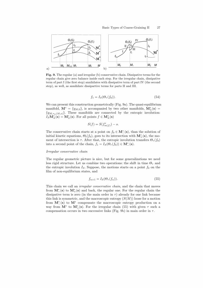
Fig. 9. The regular (a) and irregular (b) conservative chain. Dissipative terms for theregular chain give zero balance inside each step. For the irregular chain, dissipativeterm of part I (the first step) annihilates with dissipative term of part IV (the secondstep), as well, as annihilate dissipartive terms for parts II and III.
f1 = IS(Θτ (f0)). (54)
We can present this construction geometrically (Fig. 9a). The quasi-equilibriummanifold, M∗ = qM,0, is accompanied by two other manifolds, M∗
±(s) =qM,τ±(M,s). These manifolds are connected by the entropic involution:ISM∗
±(s) = M∗∓(s). For all points f ∈ M∗
±(s)
S(f) = S(f∗m(f)) − s.
The conservative chain starts at a point on f0 ∈ M∗−(s), than the solution of
initial kinetic equations, Θt(f0), goes to its intersection with M∗+(s), the mo-
ment of intersection is τ . After that, the entropic involution transfers Θτ (f0)into a second point of the chain, f1 = IS(Θτ (f0)) ∈ M∗
−(s).
Irregular conservative chain
The regular geometric picture is nice, but for some generalizations we needless rigid structure. Let us combine two operations: the shift in time Θτ andthe entropic involution IS . Suppose, the motions starts on a point f0 on thefilm of non-equilibrium states, and
fn+1 = IS(Θτ (fn)). (55)
This chain we call an irregular conservative chain, and the chain that movesfrom M∗
−(s) to M∗+(s) and back, the regular one. For the regular chain the
dissipative term is zero (in the main order in τ) already for one link becausethis link is symmetric, and the macroscopic entropy (S(M)) loose for a motionfrom M∗
−(s) to M∗ compensate the macroscopic entropy production on away from M∗ to M∗
+(s). For the irregular chain (55) with given τ such acompensation occurs in two successive links (Fig. 9b) in main order in τ .
28 Alexander N. Gorban
a)M0 M1/2 M1
f0
+ (f0)
IS
*M
*M
*M
M
(f0)
f1
Dissipation
Involution
b)M0 M1/2 M1
f0 IS( (f0))
*M
M
(f0)
f1Dissipation
Involution
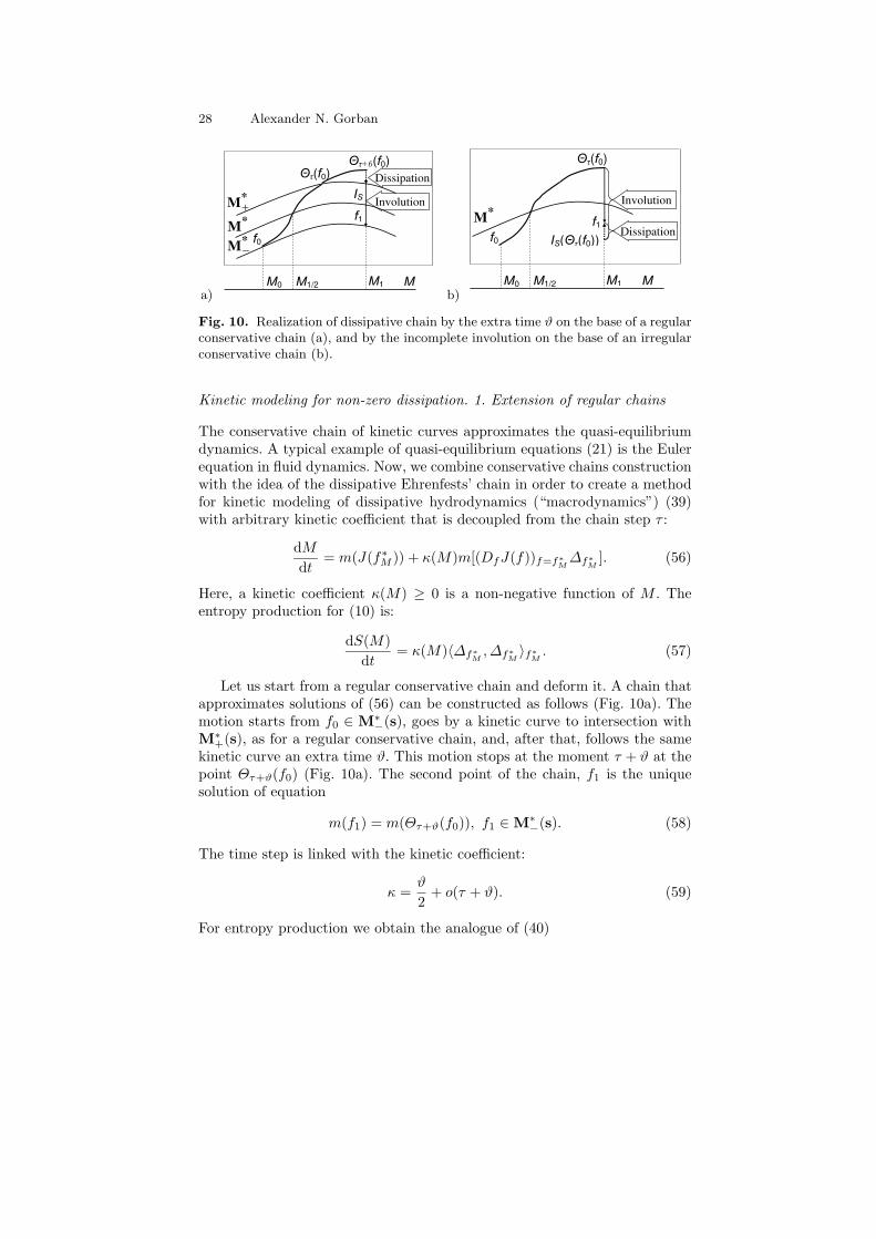
Fig. 10. Realization of dissipative chain by the extra time ϑ on the base of a regularconservative chain (a), and by the incomplete involution on the base of an irregularconservative chain (b).
Kinetic modeling for non-zero dissipation. 1. Extension of regular chains
The conservative chain of kinetic curves approximates the quasi-equilibriumdynamics. A typical example of quasi-equilibrium equations (21) is the Eulerequation in fluid dynamics. Now, we combine conservative chains constructionwith the idea of the dissipative Ehrenfests’ chain in order to create a methodfor kinetic modeling of dissipative hydrodynamics (“macrodynamics”) (39)with arbitrary kinetic coefficient that is decoupled from the chain step τ :
dM
dt= m(J(f∗
M )) + κ(M)m[(DfJ(f))f=f∗M
∆f∗M
]. (56)
Here, a kinetic coefficient κ(M) ≥ 0 is a non-negative function of M . Theentropy production for (10) is:
dS(M)
dt= κ(M)〈∆f∗
M,∆f∗
M〉f∗
M. (57)
Let us start from a regular conservative chain and deform it. A chain thatapproximates solutions of (56) can be constructed as follows (Fig. 10a). Themotion starts from f0 ∈ M∗
−(s), goes by a kinetic curve to intersection withM∗
+(s), as for a regular conservative chain, and, after that, follows the samekinetic curve an extra time ϑ. This motion stops at the moment τ + ϑ at thepoint Θτ+ϑ(f0) (Fig. 10a). The second point of the chain, f1 is the uniquesolution of equation
m(f1) = m(Θτ+ϑ(f0)), f1 ∈ M∗−(s). (58)
The time step is linked with the kinetic coefficient:
κ =ϑ
2+ o(τ + ϑ). (59)
For entropy production we obtain the analogue of (40)
Basic Types of Coarse-Graining II 29
dS(M)
dt=
ϑ
2〈∆f∗
M,∆f∗
M〉f∗
M+ o(τ + ϑ). (60)
All these formulas follow from the first–order picture. In the first order of thetime step,
qM,τ = f∗M + τ∆f∗
M;
IS(f∗M + τ∆f∗
M) = f∗
M − τ∆f∗M
;
f0 = f∗M0
− τ
2∆f∗
M0;
Θt(f0) = f∗M(t) +
(t − τ
2
)∆f∗
M0, (61)
and up to the second order of accuracy (that is, again, the first non-trivialterm)
S(qM,τ ) = S(M) +τ2
2〈∆f∗
M,∆f∗
M〉f∗
M. (62)
For a regular conservative chains, in the first order
f1 = f∗M(τ) −
τ
2∆f∗
M0. (63)
For chains (58), in the first order
f1 = f∗M(τ+ϑ) −
τ
2∆f∗
M0. (64)
Kinetic modeling for non-zero dissipation. 2. Deformed involution inirregular chains
For irregular chains, we introduce dissipation without change of the time stepτ . Let us, after entropic involution, shift the point to the quasi-equilibriumstate (Fig. 10) with some entropy increase σ(M). Because of entropy produc-tion formula (57),
σ(M) = τκ(M)〈∆f∗M
,∆f∗M〉f∗
M. (65)
This formula works, if there is sufficient amount of non-equilibrium entropy,the difference S(Mn)− S(fn) should not be too small. In average, for several(two) successive steps it should not be less than σ(M). The Ehrenfests’ chaingives a limit for possible value of κ(M) that we can realize using irregularchains with overrelaxation:
κ(M) <τ
2. (66)
Let us call the value κ(M) = τ2 the Ehrenfests’ limit. Formally, it is possible
to realize a chain of kinetic curves with time step τ for κ(M) > τ2 on the other
side of the Ehrenfests’ limit, without overrelaxation (Fig. 11).Let us choose the following notation for non-equilibrium entropy: s0 =
S(M0) − S(f0), s1 = S(M1) − S(f1), sτ (M) = τ2
2 〈∆f∗M
,∆f∗M〉f∗
M. For the
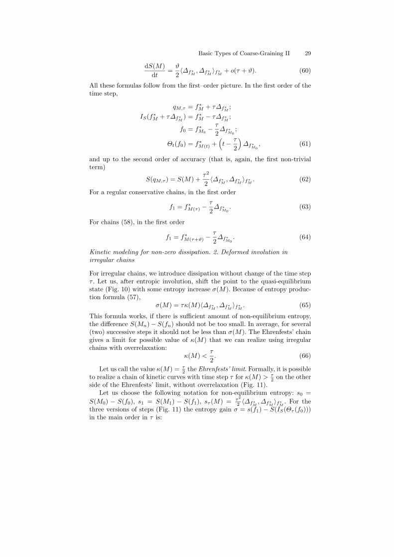
three versions of steps (Fig. 11) the entropy gain σ = s(f1) − S(IS(Θτ (f0)))in the main order in τ is:
30 Alexander N. Gorban
f0
*M
(f0)
f1
< /2
f0
(f0)
f1
= /2
f0
(f0)
f1
> /2
*M
*M
Fig. 11. The Ehrenfests’ limit of dissipation: three possible links of a dissipativechain: overrelaxation, κ(M) < τ
2(〈σ〉 = sτ − 2
√sτ 〈s0〉), Ehrenfests’ chain, κ(M) =
τ2
(σ = sτ ), and underrelaxation, κ(M) > τ2
(〈σ〉 = sτ + 2√
sτ 〈s0〉).
• For overrelaxation (κ(M) < τ2 ) σ = sτ + s0 − s1 − 2
√sτs0;
• For the Ehrenfests’ chain (full relaxation, κ(M) = τ2 ) s0 = s1 = 0 and
σ = sτ ;• For underrelaxation (κ(M) > τ
2 ) σ = sτ + s0 − s1 + 2√
sτs0.
After averaging in successive steps, the term s0 − s1 tends to zero, andwe can write the estimate of the average entropy gain 〈σ〉: for overrelaxation〈σ〉 = sτ − 2
√sτ 〈s0〉 and for underelaxation 〈σ〉 = sτ + 2
√sτ 〈s0〉.
In the really interesting physical problems the kinetic coefficient κ(M)is non-constant in space. Macroscopic variables M are functions of space,κ(M) is also a function, and it is natural to take a space-dependent step ofmacroscopic entropy production σ(M). It is possible to organize the involu-tion (incomplete involution) step at different points with different density ofentropy production step σ.
Which entropy rules the kinetic model?
For linear kinetic equations, for example, for the free flight equation (42) thereexist many concave Lyapunov functionals (for dissipative systems) or integralsof motion (for conservative systems), see, for example, (4).
There are two reasonable conditions for entropy choice: additivity withrespect to joining of independent systems, and trace form (sum or integral ofsome function h(f, f∗)). These conditions select a one-parametric family [43,44], a linear combination of the classical Boltzmann–Gibbs–Shannon entropywith h(f) = −f ln f and the Burg Entropy with h(f) = ln f , both in theKullback form:
Sα = −α
∫f ln
f
f∗dΓ (x) + (1 − α)
∫f∗ ln
f
f∗dΓ (x),
where 1 ≥ α ≥ 0, and f∗dΓ is invariant measure. Singularity of the Burg termfor f → 0 provides the positivity preservation in all entropic involutions.
Basic Types of Coarse-Graining II 31
If we weaken these conditions and require that there exists such a mono-tonic (nonlinear) transformation of entropy scale that in one scale entropy isadditive, and in transformed one it has a trace form, then we get additionallya family of Renyi–Tsallis entropies with h(f) = 1−fq
1−q [44] (these entropies and
their applications are discussed in details in [45]).Both the Renyi–Tsallis entropy and the Burge entropy are in use in the
entropic lattice Boltzmann methods from the very beginning [46, 89]. Theconnection of this entropy choice with Galilei invariance is demonstrated in[46].
Elementary examples
In the most popular and simple example, the conservative formal kineticequations (12) is the free flight equation (42). Macroscopic variables M arethe hydrodynamic fields: n(x) =
∫f(x,v) dv, n(x)u(x) =
∫vf(x,v) dv,
3n(x)kBT/2m = 12
∫v2f(x,v) dv − 1
2n(x)u2(x), where m is particle mass.In 3D at any space point we have five independent variables.
For a given value of five macroscopic variables M = n,u, T (3D), thequasi-equilibrium distribution is the classical local Maxwellian:
f∗M (x,v) = n
(2πkBT
m
)−3/2
exp
(−m(v − u)2
2kBT
), (67)
The standard choice of entropy for this example is the classical Boltzmann–Gibbs–Shannon entropy (5) with entropy density s(x). All the involution op-erations are performed pointwise: at each point x we calculate hydrodynamicmoments M , the correspondent local Maxwellian (67) f∗
M , and find the en-tropic inversion at this point with the standard entropy. For dissipative chains,it is useful to take the dissipation (the entropy density gain in one step) pro-portional to the S(M) − S(f), and not with fixed value.
The special variation of the discussed example is the free flight with finitenumber of velocities: f(x,v) =
∑i fi(x)δ(v−vi). Free flight does not change
the set of velocities v1, . . . . . . vn. If we define entropy, then we can define anequilibrium distribution for this set of velocity too. For the entropy definitionlet us substitute δ-functions in expression for f(x,v) by some “drops” withunite volume, small diameter, and fixed density that may depend on i. Afterthat, the classical entropy formula unambiguously leads to expression:
s(x) = −∑
i
fi(x)
(ln
fi(x)
f0i
− 1
). (68)
This formula is widely known in chemical kinetics (see elsewhere, for exam-ple [34–36]). After classical work of Zeldovich [37] (1938), this function isrecognized as a useful instrument for analysis of chemical kinetic equations.Vector of values f0 = f0
i gives us a “particular equilibrium:” for M = m(f0)the conditional equilibrium (s → max, M = m(f0)) is f0. With entropy (68)
32 Alexander N. Gorban
we can construct all types of conservative and dissipative chains for discreteset of velocities. If we need to approximate the continuous local equilibria andinvolutions by our discrete equilibria and involutions, then we should choosea particular equilibrium distribution
∑i f0
i δ(v − vi) in velocity space as anapproximation to the Maxwellian f∗0(v) with correspondent value of macro-scopic variables M0 calculated for the discrete distribution f0: n =
∑i f0
i ,... This approximation of distributions should be taken in the weak sense. Itmeans that vi are nodes, and f0
i are weights for a cubature formula in 3Dspace with weight f∗0(v):
∫p(v)f∗0(v) dv ≈
∑
i
p(vi)f0i . (69)
There exist a huge population of cubature formulas in 3D with Gaussianweight that are optimal in various senses [95]. Each of them contains a hintfor a choice of nodes vi and weights f0
i for the best discrete approximation ofcontinuous dynamics. Applications of this entropy (68) to the lattice Boltz-mann models are developed in [93].
There is one more opportunity to use entropy (68) and related involutionsfor discrete velocity systems. If for some of components fi = 0, then we canfind the correspondent positive equilibrium, and perform the involution in thewhole space. But there is another way: if for some of velocities fi = 0, then wecan reduce the space, and find an equilibrium for non-zero components only,for the shortened list of velocities. These boundary equilibria play importantrole in the chemical thermodynamic estimations [96].
This approach allows us to construct systems with variable in space setof velocities. There could be “soft particles” with given velocities, and thedensity distribution in these particles changes only when several particlescollide. In 3D for the possibility of a non-trivial equilibrium that does notobligatory coincide with the current distribution we need more than 5 differentvelocity vectors, hence, a non-trivial collision (≈ entropic inversion) is possibleonly for 6 one-velocity particles. If in a collision participate 5 one-velocityparticles or less, then they are just transparent and don’t interact at all. Formore moments, if we add some additional fields (stress tensor, for example),the number of velocity vectors that is necessary for non-trivial involutionincreases.
Lattice Boltzmann models: lattice is not a tool for discretization
In this section, we presented the theoretical backgrounds of kinetic modeling.These problems were discussed previously for development of lattice Boltz-mann methods in computational fluid dynamics. The “overrelaxation” ap-peared in [88]. In papers [90, 91] the overrelaxation based method for theNavier–Stokes equations was further developed, and the entropic involutionwas invented in [89]. Due to historical reasons, we propose to call it the Karlin–Succi involution. The problem of computational stability of entropic lattice
Basic Types of Coarse-Graining II 33
Boltzmann methods was systematically analyzed in [93,94]. H-theorem for lat-tice Boltzmann schemes was presented with details and applications in [92].For further discussion and references we address to [19].
In order to understand links from the Ehrenfests’ chains to the latticeBoltzmann models, let us take the model with finite number of velocity vec-tors and entropy (68). Let the velocities from the set v1, . . . . . . vn be auto-morphisms of some lattice L: L + vi = L. Then the restriction of free flightin time τ on the functions on the lattice τL is exact. It means that the freeflight shift in time τ , f(x, v) 7→ f(x − vτ, v) is defined on functions on thelattice, because viτ are automorphisms of τL. The entropic involution (com-plete or incomplete one) acts pointwise, hence, the restriction of the chainson the lattice τL is exact too. In that sense, the role of lattice here is essen-tially different from the role of grid in numerical methods for PDE. All thediscretization contains in the velocity set v1, . . . . . . vn, and the accuracy ofdiscretization is the accuracy of cubature formulas (69).
The lattice τL is a tool for presentation of velocity set as a subset of L
automorphism group. At the same time, it is a perfect screen for presentationof the chain dynamics, because restriction of that dynamics on this lattice isan autonomous dynamic of lattice distribution. (Here we meet a rather rarecase of exact model reduction.)
The boundary conditions for the lattice Boltzmann models deserve specialattention. There were many trials of non-physical conditions until the proper(and absolutely natural) discretization of well-known classical kinetic bound-ary conditions (see, for example, [80]) were proposed [97]. It is necessary andsufficient just to describe scattering of particles on the boundary with maxi-mal possible respect to the basic physics (and given proportion between elasticcollisions and thermalization).
3 Coarse-graining by filtering
The most popular area for filtering applications in mathematical physics isthe Large Eddy Simulation (LES) in fluid dynamics [17]. Perhaps, the firstattempt to turbulence modeling was done by Boussinesq in 1887. After that,Taylor (1921, 1935, 1938) and Kolmogorov (1941) have provided the bases ofthe statistical theory of turbulence. The Kolmogorov theory of turbulence selfsimilarity inspired many attempts of so-called subgrid-scale modeling (SGSmodel): only the large scale motions of the flow are solved by filtering out thesmall and universal eddies. For the dynamic subgrid-scale models a filteringstep is required to compute the SGS stress tensor. The filtering a hydrody-namic field is defined as convoluting the field functions with a filtering kernel,as it is done in electrical engineering:
n, nu, nT(x) =
∫G(x − y)n, nu, nT(y) dy. (70)
34 Alexander N. Gorban
Various filter kernels are in use. Most popular of them are:
1. The box filter G(x) = H(∆/2 − |x|)/∆;2. The Gaussian filter G(x) = 1
∆
√6/π exp (−6x2/∆2),
where ∆ is the filter width (for the Gaussian filter, ∆/2 =√
3σ, this conven-tion corresponds to 91.6% of probability in the interval [−∆/2,+∆/2] for theGaussian distribution) , H is the Heaviside function, G(x) =
∏i G(xi).
In practical applications, implicit filtering is sometimes done by the griditself. This filtering by grids should be discussed in context of the Whittaker–Nyquist–Kotelnikov–Shannon sampling theory [98,99]. Bandlimited functions(that is, functions which Fourier transform has compact support) can be ex-actly reconstructed from their values on a sufficiently fine grid by the Nyquist-Shannon interpolation formula and its multidimensional analogues. If, in 1D,the Fourier spectrum of f(x) belongs to the interval [−kmax, kmax], and thegrid step h is less than π/kmax (it is, twice less than the minimal wave length),then this formula gives the exact representation of f(x) for all points x:
f(x) =
+∞∑
n=−∞
f(nh)sinc(π
[x
h− n
]), (71)
where sinc(x) = sin xx . That interpolation formula implies an exact differenti-
ation formula in the nodes:
df(x)
dx
∣∣∣∣x=nh
= 2π∞∑
k=1
(−1)k+1 f((n + k)h) − f((n − k)h)
2kh. (72)
Such “long tail” exact differentiation formulas are useful under assumptionabout bounded Fourier spectrum.
As a background for SGS modeling, the Boussinesq hypothesis is widelyused. This hypothesis is that the turbulent terms can be modeled as di-rectly analogues to the molecular viscosity terms using a “turbulent viscosity.”Strictly speaking, no hypothesis are needed for equation filtering, and below asketch of exact filtering theory for kinetic equations is presented. The idea ofreversible regularization without apriory closure assumptions in fluid dynam-ics was proposed by Leray [13]. Now it becomes popular again [100,102,103].
3.1 Filtering as auxiliary kinetics
Idea of filtering in kinetics
The variety of possible filters is too large, and we need some fundamentalconditions that allow to select physically reasonable approach.
Let us start again from the formal kinetic equation (12) df/dt = J(f)with concave entropy functional S(f) that does not increase in time and isdefined in a convex subset U of a vector space E.
The filter transformation Φ∆ : U → U , where ∆ is the filter width, shouldsatisfy the following conditions:
Basic Types of Coarse-Graining II 35
1. Preservation of conservation laws: for any basic conservation law of theform C[f ] = const filtering does not change the value C[f ]: C[Φ∆(f)] =C[f ]. This condition should be satisfied for the whole probability or fornumber of particles (in most of classical situations), momentum, energy,and filtering should not change the center of mass, this is not so widelyknown condition, but physically obvious consequence of Galilei invariance.
2. The Second Law (entropy growth): S(Φ∆(f)) ≥ S(f).
It is easy to check the conservation laws for convoluting filters (70), and herewe find the first benefit from the kinetic equation filtering: for usual kineticequations and all mentioned conservation laws functionals C[f ] are linear,and the conservation preservation conditions are very simple linear restric-tions on the kernel G (at least, far from the boundary). For example, for theBoltzmann ideal gas distribution function f(x,v), the number of particles,momentum, and energy conserve in filtering f(x,v) =
∫G(x − y)f(y,v) dy,
if∫
G(x) dx = 1; for the center of mass conservation we need also a symmetrycondition
∫xG(x) dx = 0. It is necessary to mention that usual filters extend
the support of distribution, hence, near the boundary the filters should bemodified, and boundary can violate the Galilei invariance, as well, as momen-tum conservation. We return to these problems in this paper later.
For continuum mechanics equations, energy is not a linear functional, andoperations with filters require some accuracy and additional efforts, for ex-ample, introduction of spatially variable filters [101]. Perhaps, the best wayis to lift the continuum mechanics to kinetics, to filter the kinetic equation,and then to return back to filtered continuum mechanics. On kinetic level,it becomes obvious how filtering causes the redistribution of energy betweeninternal energy and mechanical energy: energy of small eddies and of othersmall-scale inhomogeneities partially migrates into internal energy.
Filtering semigroup
If we apply the filtering twice, it should lead just just to increase of the filterwidth. This natural semigroup condition reduces the set of allowed filterssignificantly. The approach based on filters superposition was analyzed byGermano [15] and developed by many successors. Let us formalize it in a form
Φ∆′(Φ∆(f)) = Φ∆′′(f), (73)
where ∆′′(∆′,∆) is a monotonic function, ∆′′ ≥ ∆′ and ∆′′ ≥ ∆.The semigroup condition (73) holds for the Gaussian filter with ∆′′2 =
∆′2 +∆2, and does not hold for the box filter. It is convenient to parameterizethe semigroup Φ∆|∆ ≥ 0 by an additive parameter η ≥ 0 (“auxiliary time”):∆ = ∆(η), Φη Φη′ = Φη+η′ , Φ0 = id. Further we use this parameterization.
Auxiliary kinetic equation
The filtered distribution f(η) = Φη(f0) satisfies differential equation
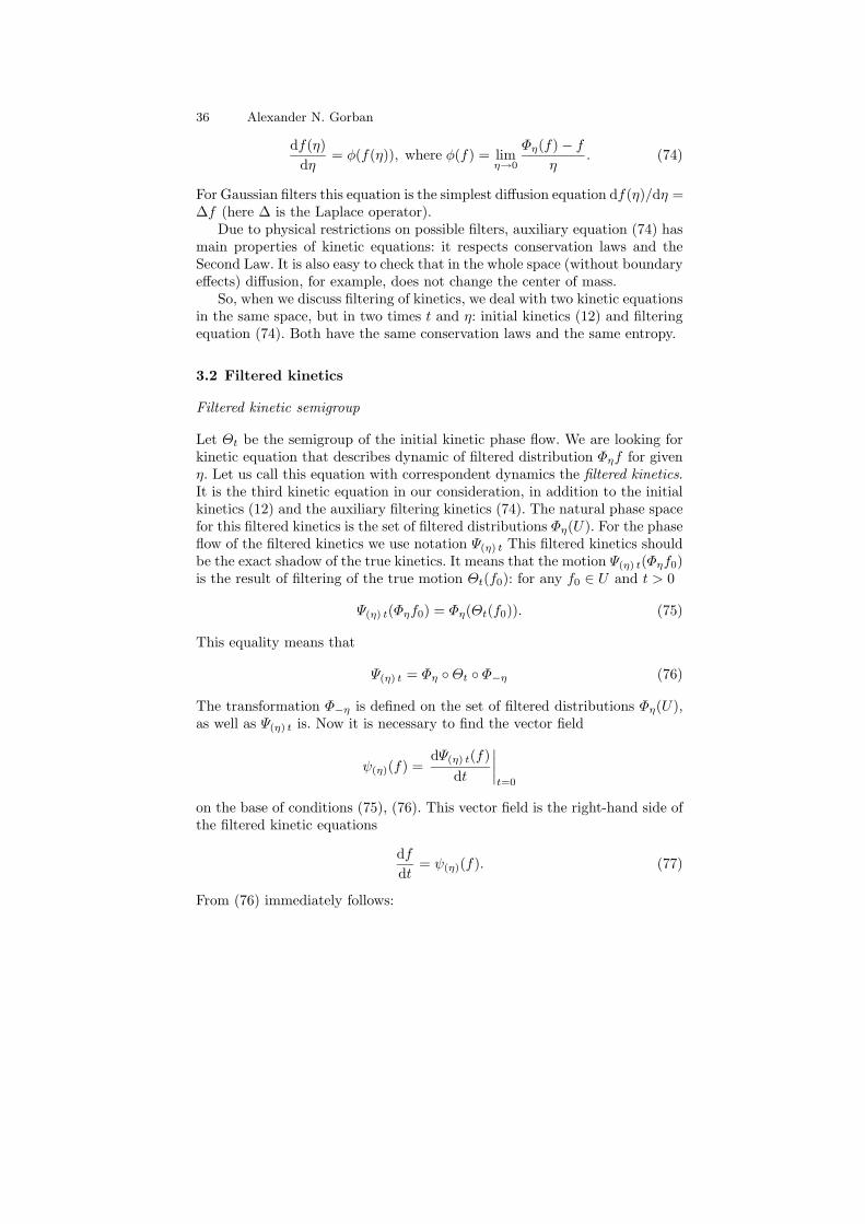
36 Alexander N. Gorban
df(η)
dη= φ(f(η)), where φ(f) = lim
η→0
Φη(f) − f
η. (74)
For Gaussian filters this equation is the simplest diffusion equation df(η)/dη =∆f (here ∆ is the Laplace operator).
Due to physical restrictions on possible filters, auxiliary equation (74) hasmain properties of kinetic equations: it respects conservation laws and theSecond Law. It is also easy to check that in the whole space (without boundaryeffects) diffusion, for example, does not change the center of mass.
So, when we discuss filtering of kinetics, we deal with two kinetic equationsin the same space, but in two times t and η: initial kinetics (12) and filteringequation (74). Both have the same conservation laws and the same entropy.
3.2 Filtered kinetics
Filtered kinetic semigroup
Let Θt be the semigroup of the initial kinetic phase flow. We are looking forkinetic equation that describes dynamic of filtered distribution Φηf for givenη. Let us call this equation with correspondent dynamics the filtered kinetics.It is the third kinetic equation in our consideration, in addition to the initialkinetics (12) and the auxiliary filtering kinetics (74). The natural phase spacefor this filtered kinetics is the set of filtered distributions Φη(U). For the phaseflow of the filtered kinetics we use notation Ψ(η) t This filtered kinetics shouldbe the exact shadow of the true kinetics. It means that the motion Ψ(η) t(Φηf0)is the result of filtering of the true motion Θt(f0): for any f0 ∈ U and t > 0
Ψ(η) t(Φηf0) = Φη(Θt(f0)). (75)
This equality means that
Ψ(η) t = Φη Θt Φ−η (76)
The transformation Φ−η is defined on the set of filtered distributions Φη(U),as well as Ψ(η) t is. Now it is necessary to find the vector field
ψ(η)(f) =dΨ(η) t(f)
dt
∣∣∣∣t=0
on the base of conditions (75), (76). This vector field is the right-hand side ofthe filtered kinetic equations
df
dt= ψ(η)(f). (77)
From (76) immediately follows:
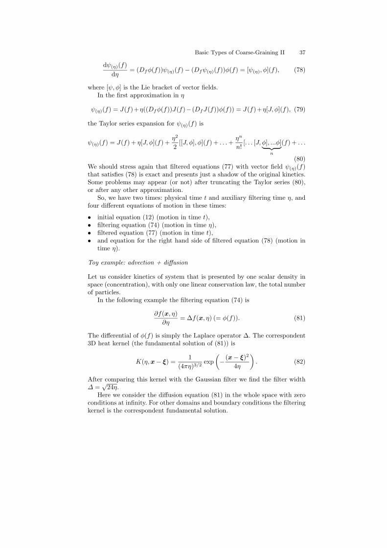
Basic Types of Coarse-Graining II 37
dψ(η)(f)
dη= (Dfφ(f))ψ(η)(f) − (Dfψ(η)(f))φ(f) = [ψ(η), φ](f), (78)
where [ψ, φ] is the Lie bracket of vector fields.In the first approximation in η
ψ(η)(f) = J(f)+η((Dfφ(f))J(f)− (DfJ(f))φ(f)) = J(f)+η[J, φ](f), (79)
the Taylor series expansion for ψ(η)(f) is
ψ(η)(f) = J(f) + η[J, φ](f) +η2
2[[J, φ], φ](f) + . . . +
ηn
n![. . . [J, φ], ...φ]︸ ︷︷ ︸
n
(f) + . . .
(80)We should stress again that filtered equations (77) with vector field ψ(η)(f)that satisfies (78) is exact and presents just a shadow of the original kinetics.Some problems may appear (or not) after truncating the Taylor series (80),or after any other approximation.
So, we have two times: physical time t and auxiliary filtering time η, andfour different equations of motion in these times:
• initial equation (12) (motion in time t),• filtering equation (74) (motion in time η),• filtered equation (77) (motion in time t),• and equation for the right hand side of filtered equation (78) (motion in
time η).
Toy example: advection + diffusion
Let us consider kinetics of system that is presented by one scalar density inspace (concentration), with only one linear conservation law, the total numberof particles.
In the following example the filtering equation (74) is
∂f(x, η)
∂η= ∆f(x, η) (= φ(f)). (81)
The differential of φ(f) is simply the Laplace operator ∆. The correspondent3D heat kernel (the fundamental solution of (81)) is
K(η,x − ξ) =1
(4πη)3/2exp
(− (x − ξ)2
4η
). (82)
After comparing this kernel with the Gaussian filter we find the filter width∆ =
√24η.
Here we consider the diffusion equation (81) in the whole space with zeroconditions at infinity. For other domains and boundary conditions the filteringkernel is the correspondent fundamental solution.
38 Alexander N. Gorban
The equation for the right hand side of filtered equation (78) is
dψ(η)(f)
dη= ∆(ψ(η)(f)) − (Dfψ(η)(f))(∆f) (= [ψ, φ](f)). (83)
For the toy example we select the advection + diffusion equation
∂f(x, t)
∂t= κ∆f(x, t) − div(v(x)f(x, t)) (= J(f)). (84)
where κ > 0 is a given diffusion coefficient, v(x) is a given velocity field. Thedifferential DfJ(f) is simply the differential operator from the right handside of (84), because this vector field is linear. After simple straightforwardcalculation we obtain the first approximation (79) to the filtered equation:
[J, φ](f) = ∆(J(f)) − (DfJ(f))(∆f) = −∆[div(vf)] + div(v∆f) (85)
= div[v∆f − ∆(vf)] = −div
[f∆v + 2
∑
r
∂v
∂xr
∂f
∂xr
]
= −div(f∆v) −∑
i
∂
∂xi
[∑
r
(∂vi
∂xr+
∂vr
∂xi
)∂f
∂xr
−∑
r
∂f
∂xr
(∂vi
∂xr− ∂vr
∂xi
)]
= −∑
i
∂
∂xi
[∑
r
(∂vi
∂xr+
∂vr
∂xi
)∂f
∂xr
]−
∑
r
∂
∂xr
(f
∂divv
∂xr
).
The resulting equations in divergence form are
∂f(x, t)
∂t= J(f) + η[J, φ](f) (86)
= −div
(−κ∇f + (v + η∆v)f + 2η
∑
r
∂v
∂xr
∂f
∂xr
)
= div((κ − 2ηS(x))∇f(x, t)) − div((v(x) + η∇divv(x))f(x, t)),
where S(x) = (Sij) = 12
(∂vi
∂xj+
∂vj
∂xi
)is the strain tensor. In filtered equations
(86) the additional diffusivity tensor −2ηS(x) and the additional velocityη∇divv(x) are present. The additional diffusivity tensor −2ηS(x) may benot positive definite. The positive definiteness of the diffusivity tensor κ −2ηS(x) may be also violated. For arbitrary initial condition f0(x) it maycause some instability problems, but we should take into account that thefiltered equations (86) are defined on the space of filtered functions for givenfiltering time η. On this space the negative diffusion (∂tf = −∆f) is possibleduring time η. Nevertheless, the approximation of exponent (80) by the linear
Basic Types of Coarse-Graining II 39
term (79) can violate the balance between smoothed initial conditions andpossible negative diffusion and can cause some instabilities.
Some numerical experiments with this model (86) for incompressible flows(divv = 0) are presented in [103].
Let us discuss equation (83) in more details. We shall represent it as thedynamics of the filtered advection flux vector Π. The filtered equation forany η should have the form: ∂f/∂t = −div(−κ∇f + Π(f)), where
Π(f) =
∑
j1,j2,j3≥0
aj1j2j3(x, η)∂j1j2j3x
f(x), (87)
where
∂j1j2j3x =
(∂
∂x1
)j1 (∂
∂x2
)j2 (∂
∂x3
)j3
(88)
For coefficients aj1j2j3(x, η) equation (83) is
∂aj1j2j3(x, η)
∂η= ∆aj1j2j3(x, η) (89)
+ 2∂aj1−1 j2j3(x, η)
∂x1+ 2
∂aj1j2−1 j3(x, η)
∂x2+ 2
∂aj1j2j3−1(x, η)
∂x3.
The initial conditions are: a000(x, 0) = v(x), aj1j2j3(x, 0) = 0 if at least oneof jk > 0. Let us define formally aj1j2j3(x, η) ≡ 0 if at least one of jk isnegative.
We shall consider (89) in the whole space with appropriate conditions atinfinity. There are many representation of solution to this system. Let us usethe Fourier transformation:
∂aj1j2j3(k, η)
∂η= −k2aj1j2j3(k, η) (90)
+2i(k1aj1−1 j2j3(k, η) + k2aj1j2−1 j3(k, η) + k3aj1j2j3−1(k, η)).
Elementary straightforward calculations give us:
aj1j2j3(k, η) = (2iη)|j|e−k2η kj11 kj2
2 kj33
j1!j2!j3!v(k), (91)
where |j| = j1 + j2 + j3. To find this answer, we consider all monotonicpaths on the integer lattice from the point (0, 0, 0) to the point (j1, j2, j3). Inconcordance with (90), every such a path adds a term
(2iη)|j|
|j|! e−k2ηkj11 kj2
2 kj33 v(k)
to aj1j2j3(k, η). The number of these paths is |j|!/(j1!j2!j3!).
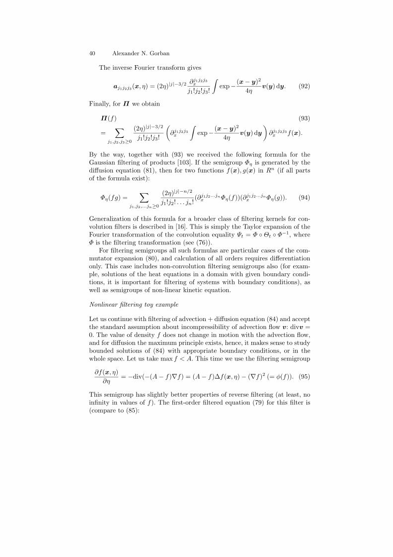
40 Alexander N. Gorban
The inverse Fourier transform gives
aj1j2j3(x, η) = (2η)|j|−3/2 ∂j1j2j3x
j1!j2!j3!
∫exp− (x − y)2
4ηv(y) dy. (92)
Finally, for Π we obtain
Π(f) (93)
=∑
j1,j2,j3≥0
(2η)|j|−3/2
j1!j2!j3!
(∂j1j2j3
x
∫exp− (x − y)2
4ηv(y) dy
)∂j1j2j3
x f(x).
By the way, together with (93) we received the following formula for theGaussian filtering of products [103]. If the semigroup Φη is generated by thediffusion equation (81), then for two functions f(x), g(x) in Rn (if all partsof the formula exist):
Φη(fg) =∑
j1,j2,...jn≥0
(2η)|j|−n/2
j1!j2! . . . jn!(∂j1j2...jn
x Φη(f))(∂j1j2...jnx Φη(g)). (94)
Generalization of this formula for a broader class of filtering kernels for con-volution filters is described in [16]. This is simply the Taylor expansion of theFourier transformation of the convolution equality Ψt = Φ Θt Φ−1, whereΦ is the filtering transformation (see (76)).
For filtering semigroups all such formulas are particular cases of the com-mutator expansion (80), and calculation of all orders requires differentiationonly. This case includes non-convolution filtering semigroups also (for exam-ple, solutions of the heat equations in a domain with given boundary condi-tions, it is important for filtering of systems with boundary conditions), aswell as semigroups of non-linear kinetic equation.
Nonlinear filtering toy example
Let us continue with filtering of advection + diffusion equation (84) and acceptthe standard assumption about incompressibility of advection flow v: divv =0. The value of density f does not change in motion with the advection flow,and for diffusion the maximum principle exists, hence, it makes sense to studybounded solutions of (84) with appropriate boundary conditions, or in thewhole space. Let us take max f < A. This time we use the filtering semigroup
∂f(x, η)
∂η= −div(−(A − f)∇f) = (A − f)∆f(x, η) − (∇f)2 (= φ(f)). (95)
This semigroup has slightly better properties of reverse filtering (at least, noinfinity in values of f). The first-order filtered equation (79) for this filter is(compare to (85):
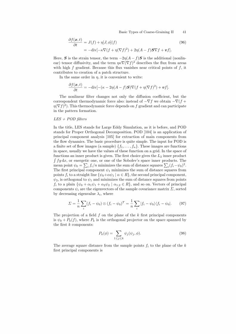
Basic Types of Coarse-Graining II 41
∂f(x, t)
∂t= J(f) + η[J, φ](f) (96)
= −div[−κ∇(f + η(∇f)2) + 2η(A − f)S∇f + vf ].
Here, S is the strain tensor, the term −2η(A− f)S is the additional (nonlin-ear) tensor diffusivity, and the term ηκ∇(∇f)2 describes the flux from areaswith high f gradient. Because this flux vanishes near critical points of f , itcontributes to creation of a patch structure.
In the same order in η, it is convenient to write:
∂f(x, t)
∂t= −div[−(κ − 2η(A − f)S)∇(f + η(∇f)2) + vf ].
The nonlinear filter changes not only the diffusion coefficient, but thecorrespondent thermodynamic force also: instead of −∇f we obtain −∇(f +η(∇f)2). This thermodynamic force depends on f gradient and can participatein the pattern formation.
LES + POD filters
In the title, LES stands for Large Eddy Simulation, as it is before, and PODstands for Proper Orthogonal Decomposition. POD [104] is an application ofprincipal component analysis [105] for extraction of main components fromthe flow dynamics. The basic procedure is quite simple. The input for POD isa finite set of flow images (a sample) f1, . . . , fn. These images are functionsin space, usually we have the values of these function on a grid. In the space offunctions an inner product is given. The first choice gives the L2 inner product∫
fg dx, or energetic one, or one of the Sobolev’s space inner products. Themean point ψ0 =
∑i fi/n minimizes the sum of distance squares
∑i(fi−ψ0)
2.The first principal component ψ1 minimizes the sum of distance squares frompoints fi to a straight line ψ0+αψ1 | α ∈ R, the second principal component,ψ2, is orthogonal to ψ1 and minimizes the sum of distance squares from pointsfi to a plain ψ0 + α1ψ1 + α2ψ2 | α1,2 ∈ R, and so on. Vectors of principalcomponents ψi are the eigenvectors of the sample covariance matrix Σ, sortedby decreasing eigenvalue λi, where
Σ =1
n
∑
i
(fi − ψ0) ⊗ (fi − ψ0)T =
1
n
∑
i
|fi − ψ0〉〈fi − ψ0|. (97)
The projection of a field f on the plane of the k first principal componentsis ψ0 + Pk(f), where Pk is the orthogonal projector on the space spanned bythe first k components:
Pk(φ) =∑
1≤j≤k
ψj(ψj , φ). (98)
The average square distance from the sample points fi to the plane of the kfirst principal components is
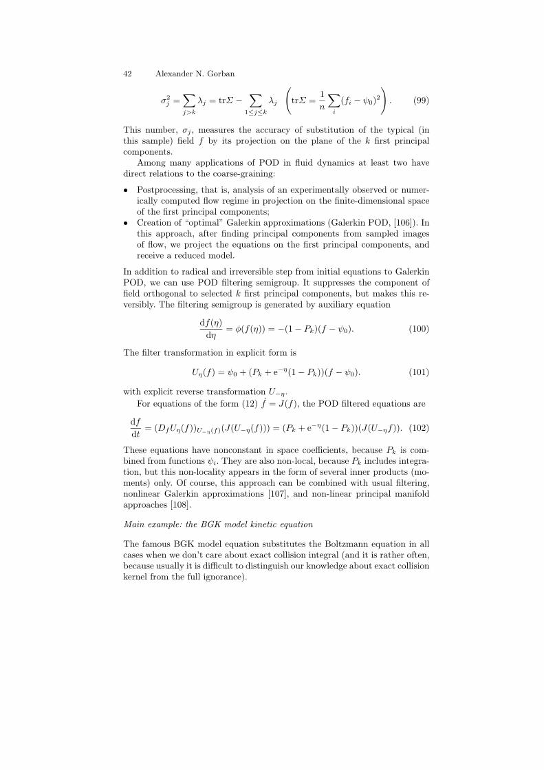
42 Alexander N. Gorban
σ2j =
∑
j>k
λj = trΣ −∑
1≤j≤k
λj
(trΣ =
1
n
∑
i
(fi − ψ0)2
). (99)
This number, σj , measures the accuracy of substitution of the typical (inthis sample) field f by its projection on the plane of the k first principalcomponents.
Among many applications of POD in fluid dynamics at least two havedirect relations to the coarse-graining:
• Postprocessing, that is, analysis of an experimentally observed or numer-ically computed flow regime in projection on the finite-dimensional spaceof the first principal components;
• Creation of “optimal” Galerkin approximations (Galerkin POD, [106]). Inthis approach, after finding principal components from sampled imagesof flow, we project the equations on the first principal components, andreceive a reduced model.
In addition to radical and irreversible step from initial equations to GalerkinPOD, we can use POD filtering semigroup. It suppresses the component offield orthogonal to selected k first principal components, but makes this re-versibly. The filtering semigroup is generated by auxiliary equation
df(η)
dη= φ(f(η)) = −(1 − Pk)(f − ψ0). (100)
The filter transformation in explicit form is
Uη(f) = ψ0 + (Pk + e−η(1 − Pk))(f − ψ0). (101)
with explicit reverse transformation U−η.
For equations of the form (12) f = J(f), the POD filtered equations are
df
dt= (DfUη(f))U−η(f)(J(U−η(f))) = (Pk + e−η(1 − Pk))(J(U−ηf)). (102)
These equations have nonconstant in space coefficients, because Pk is com-bined from functions ψi. They are also non-local, because Pk includes integra-tion, but this non-locality appears in the form of several inner products (mo-ments) only. Of course, this approach can be combined with usual filtering,nonlinear Galerkin approximations [107], and non-linear principal manifoldapproaches [108].
Main example: the BGK model kinetic equation
The famous BGK model equation substitutes the Boltzmann equation in allcases when we don’t care about exact collision integral (and it is rather often,because usually it is difficult to distinguish our knowledge about exact collisionkernel from the full ignorance).
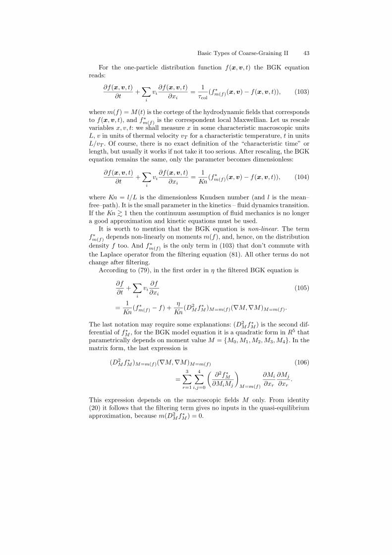
Basic Types of Coarse-Graining II 43
For the one-particle distribution function f(x,v, t) the BGK equationreads:
∂f(x,v, t)
∂t+
∑
i
vi∂f(x,v, t)
∂xi=
1
τcol(f∗
m(f)(x,v) − f(x,v, t)), (103)
where m(f) = M(t) is the cortege of the hydrodynamic fields that correspondsto f(x,v, t), and f∗
m(f) is the correspondent local Maxwellian. Let us rescalevariables x, v, t: we shall measure x in some characteristic macroscopic unitsL, v in units of thermal velocity vT for a characteristic temperature, t in unitsL/vT . Of course, there is no exact definition of the “characteristic time” orlength, but usually it works if not take it too serious. After rescaling, the BGKequation remains the same, only the parameter becomes dimensionless:
∂f(x,v, t)
∂t+
∑
i
vi∂f(x,v, t)
∂xi=
1
Kn(f∗
m(f)(x,v) − f(x,v, t)), (104)
where Kn = l/L is the dimensionless Knudsen number (and l is the mean–free–path). It is the small parameter in the kinetics – fluid dynamics transition.If the Kn & 1 then the continuum assumption of fluid mechanics is no longera good approximation and kinetic equations must be used.
It is worth to mention that the BGK equation is non-linear. The termf∗
m(f) depends non-linearly on moments m(f), and, hence, on the distribution
density f too. And f∗m(f) is the only term in (103) that don’t commute with
the Laplace operator from the filtering equation (81). All other terms do notchange after filtering.
According to (79), in the first order in η the filtered BGK equation is
∂f
∂t+
∑
i
vi∂f
∂xi(105)
=1
Kn(f∗
m(f) − f) +η
Kn(D2
Mf∗M )M=m(f)(∇M,∇M)M=m(f).
The last notation may require some explanations: (D2Mf∗
M ) is the second dif-ferential of f∗
M , for the BGK model equation it is a quadratic form in R5 thatparametrically depends on moment value M = M0,M1,M2,M3,M4. In thematrix form, the last expression is
(D2Mf∗
M )M=m(f)(∇M,∇M)M=m(f) (106)
=
3∑
r=1
4∑
i,j=0
(∂2f∗
M
∂MiMj
)
M=m(f)
∂Mi
∂xr
∂Mj
∂xr.
This expression depends on the macroscopic fields M only. From identity(20) it follows that the filtering term gives no inputs in the quasi-equilibriumapproximation, because m(D2
Mf∗M ) = 0.
44 Alexander N. Gorban
This fact is a particular case of the general commutation relations forgeneral quasi-equilibrium distributions. Let a linear operator B acts in thespace of distributions f , and there exists such a linear operator b which actsin the space of macroscopic states M that mB = bm. Then
m(Bf∗m(f) − (Dff∗
m(f))(Bf)) = 0. (107)
This means that the macroscopic projection of the Lie bracket for the vectorfields of equations ∂ηf = Bf (a field φ) and ∂tf = f∗
m(f) − f (a field θ) is
zero: m([θ, φ]) = 0.5 These commutation relations follow immediately fromthe self-consistency identities (18), (19), if we use relations mB = bm tocarry m through B. In the case of BGK equation, relations (107) hold forany linear differential or pseudodifferential operator B = Q(x, ∂/∂x) thatacts on functions of x. In this case, b = B, if we use the same notation fordifferentiation of functions and of vector-functions.
Relations (107) imply a result that deserves special efforts for physicalunderstanding: the filtered kinetic equations in zero order in the Knudsennumber produce the classical Euler equations for filtered hydrodynamic fieldswithout any trace of the filter terms. At the same time, direct filtering of theEuler equation adds new terms.
To obtain the next approximation we need the Chapman–Enskog methodfor equation (105). We developed a general method for all equations of thistype (29), and now apply this method to the filtered BGK equation. Let ustake in (26) ǫ = Kn, F (f) = F0(f) + Ffilt(f), where F0 = −v∂/∂x is the freeflight operator and
Ffilt(f) =η
Kn(D2
Mf∗M )M=m(f)(∇M,∇M)M=m(f). (108)
In these notations, for the zero term in the Chapman–Enskog expansion we
have f(0)M = f∗
M , and for the first term
f(1)M = fNS
M + ffiltM = ∆NS
f∗M
+ ∆filtf∗
M, (109)
fNSM = ∆NS
f∗M
= F0(f∗M ) − (DMf∗
M )(m(F0(f∗M )))
ffiltM = ∆filt
f∗M
= Ffilt(f) (because m(Ffilt(f)) = 0),
where NS stands for Navier–Stokes. The correspondent continuum equations(30) are
dM
dt= m(F0(f
∗M )) + Kn m(F0(∆
NSf∗
M+ ∆filt
f∗M
)). (110)
Here, the first term includes non-dissipative terms (the Euler ones) of theNavier–Stokes equations, and the second term includes both the dissipativeterms of the Navier–Stokes equations and the filtering terms. Let us collectall the classical hydrodynamic terms together:
5 The term −f gives zero input in these Lie brackets for any linear operator B.
Basic Types of Coarse-Graining II 45
∂M(x, t)
∂t= . . . . . . . . . . . .︸ ︷︷ ︸
NS terms
+Kn m
(v
∂
∂xFfilt(f)
)(111)
= . . . . . . . . . . . .︸ ︷︷ ︸NS terms
+ηm
v
∂
∂x
3∑
r=1
4∑
i,j=0
∂2f∗M
∂MiMj
∂Mi
∂xr
∂Mj
∂xr
,
The NS terms here are the right hand sides of the Navier–Stokes equationsfor the BGK kinetics (45) (with τ = 2τcol = 2Kn). Of course, (111) is one ofthe tensor viscosity – tensor diffusivity models. Its explicit form for the BGKequation and various similar model equations requires several quadratures:
Cij = m
v
∂
∂x
3∑
r=1
4∑
i,j=0
∂2f∗M
∂MiMj
(112)
(for the Maxwell distributions f∗M that are just Gaussian integrals).
Entropic stability condition for the filtered kinetic equations
Instability of filtered equations is a well-known problem. It arises becausethe reverse filtering is an ill-posed operation, the balance between filter andreverse filter in (76) may be destroyed by any approximation, as well as aperturbation may move the hydrodynamic field out of space of pre-filteredfields. (And the general filtered equations are applicable for sure in that spaceonly.)
Analysis of entropy production is the first tool for stability check. This is amain thermodynamic realization of the Lyapunov functions method (inventedin physics before Lyapunov).
The filtration term Ffilt(f) (108) in the filtered BGK equation (105) doesnot produce the Boltzmann (i.e. macroscopic) entropy S(f∗
m(f)), but is notconservative. In more details:
1. (DMS(f∗M ))(m(Ffilt(f
∗m(f)))) ≡ 0, because m(Ffilt(f)) ≡ 0;
2. (DfS(f))f∗m(f)
(Ffilt(f∗m(f))) = (DMS(f∗
M ))(m(Ffilt(f∗m(f)))) ≡ 0;
3. (DfS(f))f∗m(f)
(Ffilt(f)) = (DfS(f))f∗m(f)
(Ffilt(f∗m(f))) ≡ 0, because Ffilt(f)
depends on f∗m(f) only;
4. But for any field Ffilt(f) that depends on f∗m(f) only, if the conservativ-
ity identity (32) (DfS(f))f (Ffilt(f)) ≡ 0 is true even in a small vicinityof quasi-equilibria, then Ffilt(f) ≡ 0. Hence, the non-trivial filter termFfilt(f) cannot be conservative, the whole field F (f) = F0(f) + Ffilt(f) isnot conservative, and we cannot use the entropy production formula (31).
Instead of (31) we obtain
dS(M)
dt= Kn〈∆NS
f∗M
,∆NSf∗
M〉f∗
M+ η〈∆NS
f∗M
,∆filtf∗
M〉f∗
M. (113)
46 Alexander N. Gorban
The entropic stability condition for the filtered kinetic equations is:
dS(M)/dt ≥ 0, i.e. Kn〈∆NSf∗
M,∆NS
f∗M〉f∗
M+ η〈∆NS
f∗M
,∆filtf∗
M〉f∗
M≥ 0. (114)
There exists a plenty of convenient sufficient conditions, for example,
η ≤ Kn|〈∆NS
f∗M
,∆filtf∗
M〉f∗
M|
〈∆NSf∗
M,∆NS
f∗M〉f∗
M
; or η ≤ Kn
√√√√ 〈∆filtf∗
M,∆filt
f∗M〉f∗
M
〈∆NSf∗
M,∆NS
f∗M〉f∗
M
. (115)
The upper boundary for η that guaranties stability of the filtered equa-tions is proportional to Kn. For the Gaussian filter width ∆ this means∆ = L
√24η ∼
√Kn (where L is the characteristic macroscopic length). This
scaling, ∆/L ∼√
Kn, was discussed in [18] for moment kinetic equations be-cause different reasons: if ∆/L ≫
√Kn then the Chapman–Enskog procedure
is not applicable, and, moreover, the continuum description is probably notvalid, because the filtering term with large coefficient η violates the conditionsof hydrodynamic limit. This important remark gives the frame for η scaling,and (114), (115) give the stability boundaries inside this scale.
4 Errors of Models, ε-trajectories and Stable Properties
of Structurally Unstable Systems
4.1 Phase flow, attractors and repellers
Phase flow
In this section, we return from kinetic systems to general dynamical systems,and lose such specific tools as entropy and quasi-equilibrium. Topological dy-namics gives us a natural language for general discussion of limit behavior andrelaxation of general dynamical systems [109]. We discuss a general dynami-cal system as a semigroup of homeomorphisms (phase flow transformations):Θ(t, x) is the result of shifting point x in time t.
Let the phase space X be a compact metric space with the metrics ρ,
Θ : [0,∞[×X → X (116)
be a continuous mapping for any t ≥ 0; let mapping Θ(t, ·) : X → X behomeomorphism of X into subset of X and let these homeomorphisms formmonoparametric semigroup:
Θ(0, ·) = id, Θ(t, Θ(t′, x)) = Θ(t + t′, x) (117)
for any t, t′ ≥ 0, x ∈ X.Below we call the semigroup of mappings Θ(t, ·) a semiflow of homeomor-
phisms (or, for short, semiflow), or simply system (116). We assume that the
Basic Types of Coarse-Graining II 47
continuous map Θ(t, x) is continued to negative time t as far as it is possiblewith preservation of the semigroup property (117). For phase flow we use alsonotations Θt and Θt(x). For any given x ∈ X, x-motion is a function of timeΘ(t, x), x-motion is the whole motion if the function is defined on the wholeaxis t ∈] −∞,∞[. The image of x-motion is the x-trajectory.
Attractors and repellers
First of all, for the description of limit behaviour we need a notion of anω-limit set.
A point p ∈ X is called ω- (α-)-limit point of the x-motion (correspondinglyof the whole x-motion), if there is such a sequence tn → ∞ (tn → −∞) thatΘ(tn, x) → p as n → ∞. The totality of all ω- (α-)-limit points of x-motion iscalled its ω- (α-)-limit set and is denoted by ω(x) (α(x)).
A set W ⊂ X is called invariant set, if, for any x ∈ W , the x-motion iswhole and the whole x-trajectory belongs to W .
The sets ω(x), α(x) (the last in the case when x-motion is whole) arenonempty, closed, connected, and invariant.
The set of all ω-limit points of the system ωΘ =⋃
x∈X ω(x) is nonemptyand invariant, but may be disconnected and not closed. The sets ω(x) mightbe considered as attractors, and the sets α(x) as repellers (attractors for t →−∞). The system of these sets represents all limit behaviours of the phaseflow.
Perhaps, the most constructive idea of attractor definition combines puretopological (metric) and measure points of view. A weak attractor [113] is aclosed (invariant) set A such that the set B(A) = x | ω(x) ⊂ A (a basinof attraction) has strictly positive measure. A Milnor attractor [112] is sucha weak attractor that there is no strictly smaller closed A′ $ A so that B(A)coincides with B(A′) up to a set of measure zero. If A is a Milnor attractorand for any closed invariant proper subset A′ $ A the set B(A′) has zeromeasure, then we say that A is a minimal Milnor attractor.
Below in this section we follow a purely topological (metric) point of view,but keep in mind that its combination with measure–based ideas create aricher theory.
The dream of applied dynamics
Now we can formulate the “dream of applied dynamics.” There is such a finitenumber of invariant sets A1, . . . An that:
• Any attractor or repeller is one of the Ai;• The following relation between sets A1, . . . An is acyclic: Ai º Aj if there
exists such x that α(x) = Ai and ω(x) = Aj ;• The system A1, . . . An with the preorder Ai º Aj does not change qual-
itatively under sufficiently small perturbations of the dynamical system:all the picture can be restored by a map that is close to id.
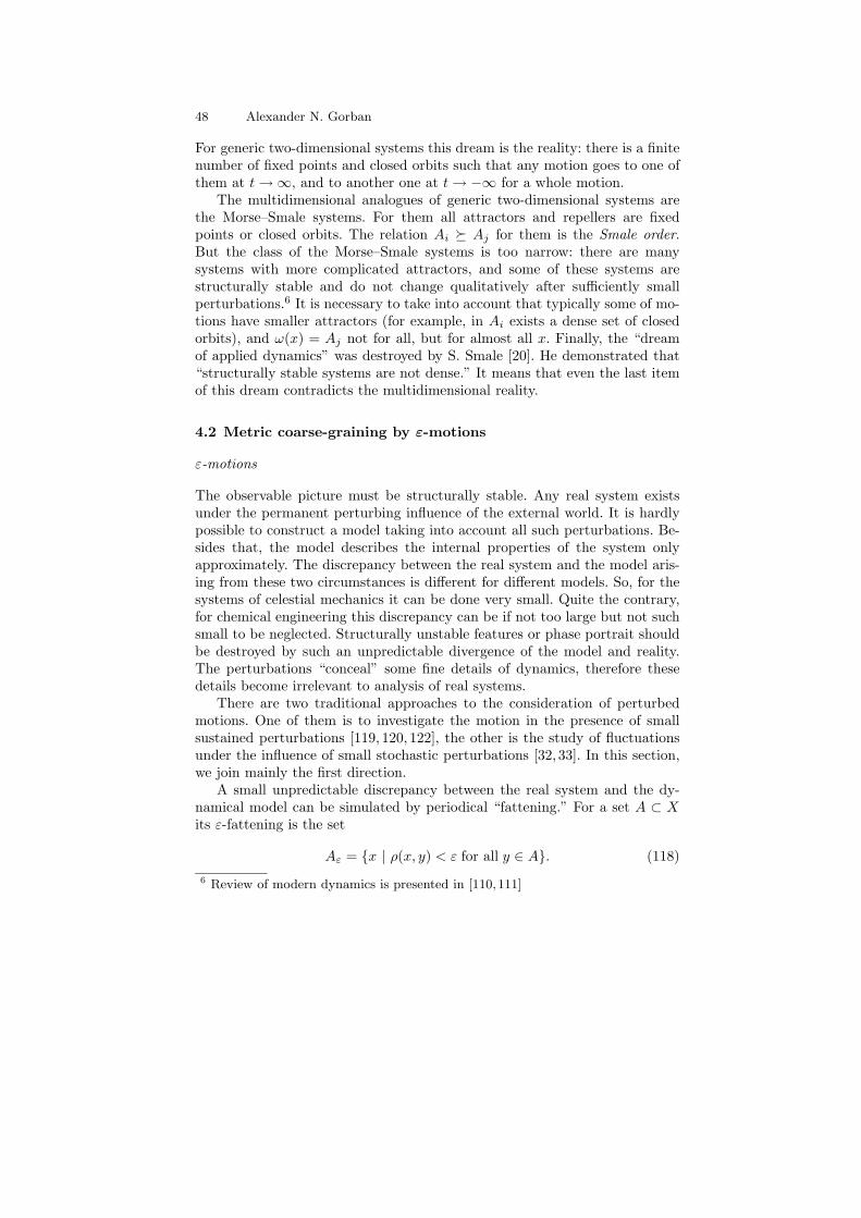
48 Alexander N. Gorban
For generic two-dimensional systems this dream is the reality: there is a finitenumber of fixed points and closed orbits such that any motion goes to one ofthem at t → ∞, and to another one at t → −∞ for a whole motion.
The multidimensional analogues of generic two-dimensional systems arethe Morse–Smale systems. For them all attractors and repellers are fixedpoints or closed orbits. The relation Ai º Aj for them is the Smale order.But the class of the Morse–Smale systems is too narrow: there are manysystems with more complicated attractors, and some of these systems arestructurally stable and do not change qualitatively after sufficiently smallperturbations.6 It is necessary to take into account that typically some of mo-tions have smaller attractors (for example, in Ai exists a dense set of closedorbits), and ω(x) = Aj not for all, but for almost all x. Finally, the “dreamof applied dynamics” was destroyed by S. Smale [20]. He demonstrated that“structurally stable systems are not dense.” It means that even the last itemof this dream contradicts the multidimensional reality.
4.2 Metric coarse-graining by ε-motions
ε-motions
The observable picture must be structurally stable. Any real system existsunder the permanent perturbing influence of the external world. It is hardlypossible to construct a model taking into account all such perturbations. Be-sides that, the model describes the internal properties of the system onlyapproximately. The discrepancy between the real system and the model aris-ing from these two circumstances is different for different models. So, for thesystems of celestial mechanics it can be done very small. Quite the contrary,for chemical engineering this discrepancy can be if not too large but not suchsmall to be neglected. Structurally unstable features or phase portrait shouldbe destroyed by such an unpredictable divergence of the model and reality.The perturbations “conceal” some fine details of dynamics, therefore thesedetails become irrelevant to analysis of real systems.
There are two traditional approaches to the consideration of perturbedmotions. One of them is to investigate the motion in the presence of smallsustained perturbations [119, 120, 122], the other is the study of fluctuationsunder the influence of small stochastic perturbations [32, 33]. In this section,we join mainly the first direction.
A small unpredictable discrepancy between the real system and the dy-namical model can be simulated by periodical “fattening.” For a set A ⊂ Xits ε-fattening is the set
Aε = x | ρ(x, y) < ε for all y ∈ A. (118)
6 Review of modern dynamics is presented in [110,111]
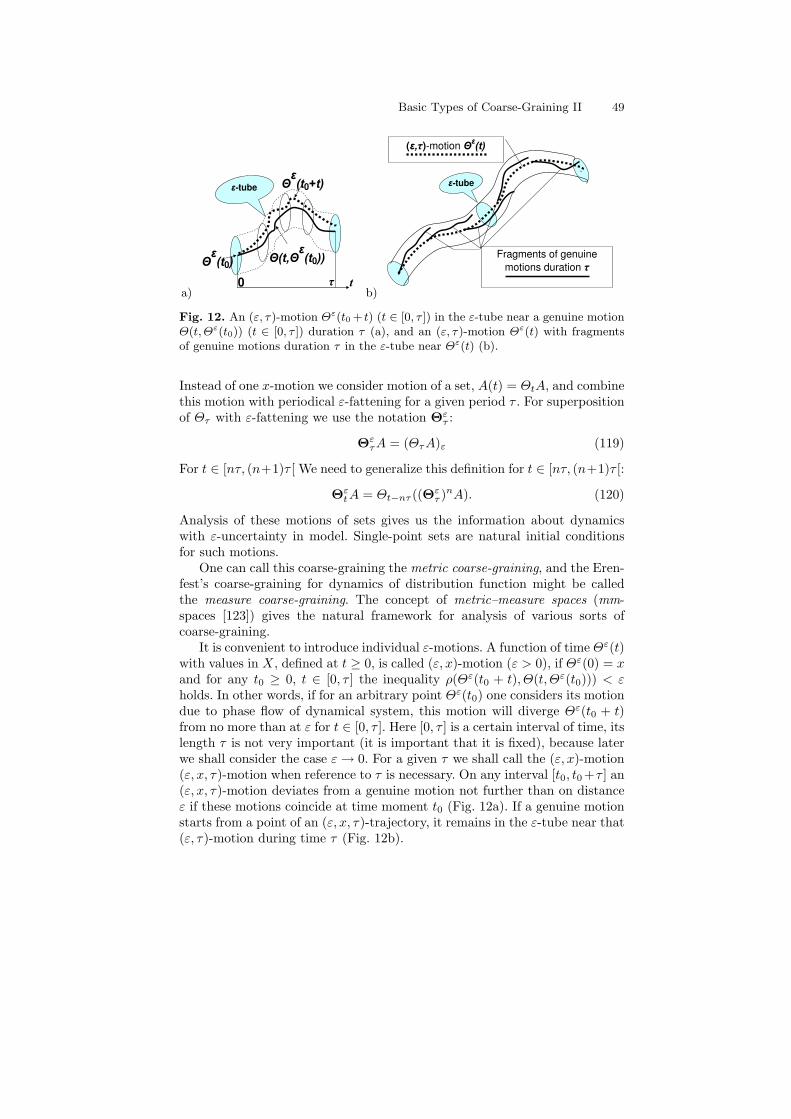
Basic Types of Coarse-Graining II 49
a)
(t0)
-tube
(t, (t0))
(t0+t)
0 t
b)
-tube
( , )-motion (t)
Fragments of genuine
motions duration
Fig. 12. An (ε, τ)-motion Θε(t0 + t) (t ∈ [0, τ ]) in the ε-tube near a genuine motionΘ(t, Θε(t0)) (t ∈ [0, τ ]) duration τ (a), and an (ε, τ)-motion Θε(t) with fragmentsof genuine motions duration τ in the ε-tube near Θε(t) (b).
Instead of one x-motion we consider motion of a set, A(t) = ΘtA, and combinethis motion with periodical ε-fattening for a given period τ . For superpositionof Θτ with ε-fattening we use the notation Θε
τ :
ΘετA = (ΘτA)ε (119)
For t ∈ [nτ, (n+1)τ [ We need to generalize this definition for t ∈ [nτ, (n+1)τ [:
ΘεtA = Θt−nτ ((Θε
τ )nA). (120)
Analysis of these motions of sets gives us the information about dynamicswith ε-uncertainty in model. Single-point sets are natural initial conditionsfor such motions.
One can call this coarse-graining the metric coarse-graining, and the Eren-fest’s coarse-graining for dynamics of distribution function might be calledthe measure coarse-graining. The concept of metric–measure spaces (mm-spaces [123]) gives the natural framework for analysis of various sorts ofcoarse-graining.
It is convenient to introduce individual ε-motions. A function of time Θε(t)with values in X, defined at t ≥ 0, is called (ε, x)-motion (ε > 0), if Θε(0) = xand for any t0 ≥ 0, t ∈ [0, τ ] the inequality ρ(Θε(t0 + t), Θ(t, Θε(t0))) < εholds. In other words, if for an arbitrary point Θε(t0) one considers its motiondue to phase flow of dynamical system, this motion will diverge Θε(t0 + t)from no more than at ε for t ∈ [0, τ ]. Here [0, τ ] is a certain interval of time, itslength τ is not very important (it is important that it is fixed), because laterwe shall consider the case ε → 0. For a given τ we shall call the (ε, x)-motion(ε, x, τ)-motion when reference to τ is necessary. On any interval [t0, t0 +τ ] an(ε, x, τ)-motion deviates from a genuine motion not further than on distanceε if these motions coincide at time moment t0 (Fig. 12a). If a genuine motionstarts from a point of an (ε, x, τ)-trajectory, it remains in the ε-tube near that(ε, τ)-motion during time τ (Fig. 12b).
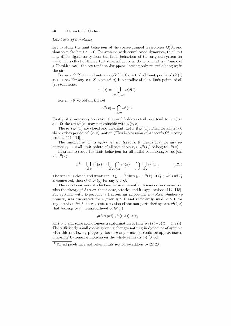
50 Alexander N. Gorban
Limit sets of ε-motions
Let us study the limit behaviour of the coarse-grained trajectories ΘεtA, and
than take the limit ε → 0. For systems with complicated dynamics, this limitmay differ significantly from the limit behaviour of the original system forε = 0. This effect of the perturbation influence in the zero limit is a “smile ofa Cheshire cat:” the cat tends to disappear, leaving only its smile hanging inthe air.
For any Θε(t) the ω-limit set ω(Θε) is the set of all limit points of Θε(t)at t → ∞. For any x ∈ X a set ωε(x) is a totality of all ω-limit points of all(ε, x)-motions:
ωε(x) =⋃
Θε(0)=x
ω(Θε).
For ε → 0 we obtain the set
ω0(x) =⋂
ε>0
ωε(x).
Firstly, it is necessary to notice that ωε(x) does not always tend to ω(x) asε → 0: the set ω0(x) may not coincide with ω(x, k).
The sets ω0(x) are closed and invariant. Let x ∈ ω0(x). Then for any ε > 0there exists periodical (ε, x)-motion (This is a version of Anosov’s C0-closinglemma [111,114]).
The function ω0(x) is upper semicontinuous. It means that for any se-quence xi → x all limit points of all sequences yi ∈ ω0(xi) belong to ω0(x).
In order to study the limit behaviour for all initial conditions, let us joinall ω0(x):
ω0 =⋃
x∈X
ω0(x) =⋃
x∈X
⋂
ε>0
ωε(x) =⋂
ε>0
⋃
x∈X
ωε(x). (121)
The set ω0 is closed and invariant. If y ∈ ω0 then y ∈ ω0(y). If Q ⊂ ω0 and Qis connected, then Q ⊂ ω0(y) for any y ∈ Q.7
The ε-motions were studied earlier in differential dynamics, in connectionwith the theory of Anosov about ε-trajectories and its applications [114–118].For systems with hyperbolic attractors an important ε-motion shadowingproperty was discovered: for a given η > 0 and sufficiently small ε > 0 forany ε-motion Θε(t) there exists a motion of the non-perturbed system Θ(t, x)that belongs to η - neighborhood of Θε(t):
ρ(Θε(φ(t)), Θ(t, x)) < η,
for t > 0 and some monotonous transformation of time φ(t) (t−φ(t) = O(εt)).The sufficiently small coarse-graining changes nothing in dynamics of systemswith this shadowing property, because any ε-motion could be approximateduniformly by genuine motions on the whole semiaxis t ∈ [0,∞[.
7 For all proofs here and below in this section we address to [22,23].
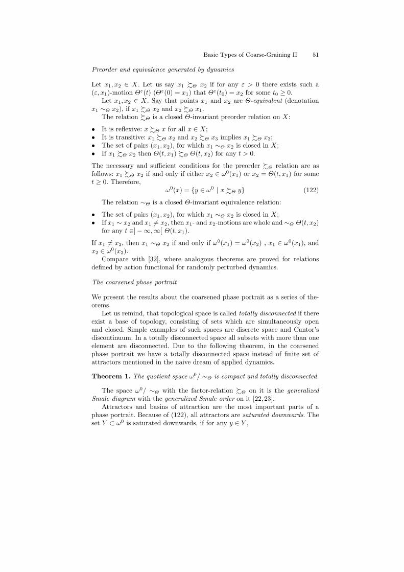
Basic Types of Coarse-Graining II 51
Preorder and equivalence generated by dynamics
Let x1, x2 ∈ X. Let us say x1 %Θ x2 if for any ε > 0 there exists such a(ε, x1)-motion Θε(t) (Θε(0) = x1) that Θε(t0) = x2 for some t0 ≥ 0.
Let x1, x2 ∈ X. Say that points x1 and x2 are Θ-equivalent (denotationx1 ∼Θ x2), if x1 %Θ x2 and x2 %Θ x1.
The relation %Θ is a closed Θ-invariant preorder relation on X:
• It is reflexive: x %Θ x for all x ∈ X;• It is transitive: x1 %Θ x2 and x2 %Θ x3 implies x1 %Θ x3;• The set of pairs (x1, x2), for which x1 ∼Θ x2 is closed in X;• If x1 %Θ x2 then Θ(t, x1) %Θ Θ(t, x2) for any t > 0.
The necessary and sufficient conditions for the preorder %Θ relation are asfollows: x1 %Θ x2 if and only if either x2 ∈ ω0(x1) or x2 = Θ(t, x1) for somet ≥ 0. Therefore,
ω0(x) = y ∈ ω0 | x %Θ y (122)
The relation ∼Θ is a closed Θ-invariant equivalence relation:
• The set of pairs (x1, x2), for which x1 ∼Θ x2 is closed in X;• If x1 ∼ x2 and x1 6= x2, then x1- and x2-motions are whole and ∼Θ Θ(t, x2)
for any t ∈] −∞,∞[ Θ(t, x1).
If x1 6= x2, then x1 ∼Θ x2 if and only if ω0(x1) = ω0(x2) , x1 ∈ ω0(x1), andx2 ∈ ω0(x2).
Compare with [32], where analogous theorems are proved for relationsdefined by action functional for randomly perturbed dynamics.
The coarsened phase portrait
We present the results about the coarsened phase portrait as a series of the-orems.
Let us remind, that topological space is called totally disconnected if thereexist a base of topology, consisting of sets which are simultaneously openand closed. Simple examples of such spaces are discrete space and Cantor’sdiscontinuum. In a totally disconnected space all subsets with more than oneelement are disconnected. Due to the following theorem, in the coarsenedphase portrait we have a totally disconnected space instead of finite set ofattractors mentioned in the naive dream of applied dynamics.
Theorem 1. The quotient space ω0/ ∼Θ is compact and totally disconnected.
The space ω0/ ∼Θ with the factor-relation %Θ on it is the generalizedSmale diagram with the generalized Smale order on it [22,23].
Attractors and basins of attraction are the most important parts of aphase portrait. Because of (122), all attractors are saturated downwards. Theset Y ⊂ ω0 is saturated downwards, if for any y ∈ Y ,
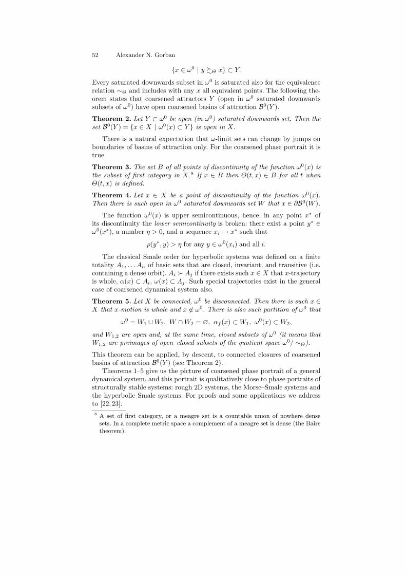
52 Alexander N. Gorban
x ∈ ω0 | y %Θ x ⊂ Y.
Every saturated downwards subset in ω0 is saturated also for the equivalencerelation ∼Θ and includes with any x all equivalent points. The following the-orem states that coarsened attractors Y (open in ω0 saturated downwardssubsets of ω0) have open coarsened basins of attraction B0(Y ).
Theorem 2. Let Y ⊂ ω0 be open (in ω0) saturated downwards set. Then theset B0(Y ) = x ∈ X | ω0(x) ⊂ Y is open in X.
There is a natural expectation that ω-limit sets can change by jumps onboundaries of basins of attraction only. For the coarsened phase portrait it istrue.
Theorem 3. The set B of all points of discontinuity of the function ω0(x) isthe subset of first category in X.8 If x ∈ B then Θ(t, x) ∈ B for all t whenΘ(t, x) is defined.
Theorem 4. Let x ∈ X be a point of discontinuity of the function ω0(x).Then there is such open in ω0 saturated downwards set W that x ∈ ∂B0(W ).
The function ω0(x) is upper semicontinuous, hence, in any point x∗ ofits discontinuity the lower semicontinuity is broken: there exist a point y∗ ∈ω0(x∗), a number η > 0, and a sequence xi → x∗ such that
ρ(y∗, y) > η for any y ∈ ω0(xi) and all i.
The classical Smale order for hyperbolic systems was defined on a finitetotality A1, . . . An of basic sets that are closed, invariant, and transitive (i.e.containing a dense orbit). Ai ≻ Aj if there exists such x ∈ X that x-trajectoryis whole, α(x) ⊂ Ai, ω(x) ⊂ Aj . Such special trajectories exist in the generalcase of coarsened dynamical system also.
Theorem 5. Let X be connected, ω0 be disconnected. Then there is such x ∈X that x-motion is whole and x 6∈ ω0. There is also such partition of ω0 that
ω0 = W1 ∪ W2, W ∩ W2 = ∅, αf (x) ⊂ W1, ω0(x) ⊂ W2,
and W1,2 are open and, at the same time, closed subsets of ω0 (it means thatW1,2 are preimages of open–closed subsets of the quotient space ω0/ ∼Θ).
This theorem can be applied, by descent, to connected closures of coarsenedbasins of attraction B0(Y ) (see Theorem 2).
Theorems 1–5 give us the picture of coarsened phase portrait of a generaldynamical system, and this portrait is qualitatively close to phase portraits ofstructurally stable systems: rough 2D systems, the Morse–Smale systems andthe hyperbolic Smale systems. For proofs and some applications we addressto [22,23].
8 A set of first category, or a meagre set is a countable union of nowhere densesets. In a complete metric space a complement of a meagre set is dense (the Bairetheorem).
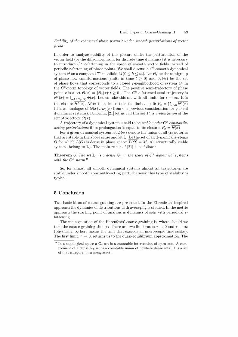
Basic Types of Coarse-Graining II 53
Stability of the coarsened phase portrait under smooth perturbations of vectorfields
In order to analyze stability of this picture under the perturbation of thevector field (or the diffeomorphism, for discrete time dynamics) it is necessaryto introduce Ck ε-fattening in the space of smooth vector fields instead ofperiodic ε-fattening of phase points. We shall discuss a Ck-smooth dynamicalsystem Θ on a compact Cm-manifold M(0 ≤ k ≤ m). Let Θt be the semigroupof phase flow transformations (shifts in time t ≥ 0) and Uε(Θ) be the setof phase flows that corresponds to a closed ε-neighborhood of system Θt inthe Ck-norm topology of vector fields. The positive semi-trajectory of phasepoint x is a set Θ(x) = Θt(x): t ≥ 0. The Ck ε-fattened semi-trajectory isΘε(x) =
⋃Φ∈Uε(Θ) Φ(x). Let us take this set with all limits for t → ∞. It is
the closure Θε(x). After that, let us take the limit ε → 0: Px =⋂
ε>0 Θε(x)(it is an analogue of Θ(x)∪ω0(x) from our previous consideration for generaldynamical systems). Following [21] let us call this set Px a prolongation of thesemi-trajectory Θ(x).
A trajectory of a dynamical system is said to be stable under Ck constantly-acting perturbations if its prolongation is equal to its closure: Px = Θ(x)
For a given dynamical system let L(Θ) denote the union of all trajectoriesthat are stable in the above sense and let L1 be the set of all dynamical systemsΘ for which L(Θ) is dense in phase space: L(Θ) = M . All structurally stablesystems belong to L1. The main result of [21] is as follows:
Theorem 6. The set L1 is a dense Gδ in the space of Ck dynamical systemswith the Ck norm.9
So, for almost all smooth dynamical systems almost all trajectories arestable under smooth constantly-acting perturbations: this type of stability istypical.
5 Conclusion
Two basic ideas of coarse-graining are presented. In the Ehrenfests’ inspiredapproach the dynamics of distributions with averaging is studied. In the metricapproach the starting point of analysis is dynamics of sets with periodical ε-fattening.
The main question of the Ehrenfests’ coarse-graining is: where should wetake the coarse-graining time τ? There are two limit cases: τ → 0 and τ → ∞(physically, ∞ here means the time that exceeds all microscopic time scales).The first limit, τ → 0, returns us to the quasi-equilibrium approximation. The
9 In a topological space a Gδ set is a countable intersection of open sets. A com-plement of a dense Gδ set is a countable union of nowhere dense sets. It is a setof first category, or a meagre set.
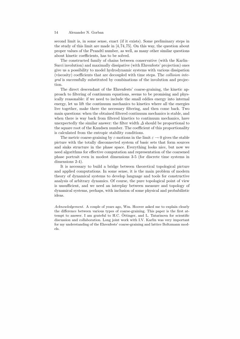
54 Alexander N. Gorban
second limit is, in some sense, exact (if it exists). Some preliminary steps inthe study of this limit are made in [4,74,75]. On this way, the question aboutproper values of the Prandtl number, as well, as many other similar questionsabout kinetic coefficients, has to be solved.
The constructed family of chains between conservative (with the Karlin–Succi involution) and maximally dissipative (with Ehrenfests’ projection) onesgive us a possibility to model hydrodynamic systems with various dissipation(viscosity) coefficients that are decoupled with time steps. The collision inte-gral is successfully substituted by combinations of the involution and projec-tion.
The direct descendant of the Ehrenfests’ coarse-graining, the kinetic ap-proach to filtering of continuum equations, seems to be promising and phys-ically reasonable: if we need to include the small eddies energy into internalenergy, let us lift the continuum mechanics to kinetics where all the energieslive together, make there the necessary filtering, and then come back. Twomain questions: when the obtained filtered continuum mechanics is stable, andwhen there is way back from filtered kinetics to continuum mechanics, haveunexpectedly the similar answer: the filter width ∆ should be proportional tothe square root of the Knudsen number. The coefficient of this proportionalityis calculated from the entropic stability conditions.
The metric coarse-graining by ε-motions in the limit ε → 0 gives the stablepicture with the totally disconnected system of basic sets that form sourcesand sinks structure in the phase space. Everything looks nice, but now weneed algorithms for effective computation and representation of the coarsenedphase portrait even in modest dimensions 3-5 (for discrete time systems indimensions 2-4).
It is necessary to build a bridge between theoretical topological pictureand applied computations. In some sense, it is the main problem of moderntheory of dynamical systems to develop language and tools for constructiveanalysis of arbitrary dynamics. Of course, the pure topological point of viewis unsufficient, and we need an interplay between measure and topology ofdynamical systems, perhaps, with inclusion of some physical and probabilisticideas.
Acknowledgement. A couple of years ago, Wm. Hoover asked me to explain clearlythe difference between various types of coarse-graining. This paper is the first at-tempt to answer. I am grateful to H.C. Ottinger, and L. Tatarinova for scientificdiscussion and collaboration. Long joint work with I.V. Karlin was very importantfor my understanding of the Ehrenfests’ coarse-graining and lattice Boltzmann mod-els.
Basic Types of Coarse-Graining II 55
References
1. P. Ehrenfest, T. Ehrenfest-Afanasyeva, The Conceptual Foundations of theStatistical Approach in Mechanics, In: Mechanics Enziklopadie der Mathe-
matischen Wissenschaften, Vol. 4., Leipzig, 1911. (Reprinted: P. Ehrenfest,T. Ehrenfest-Afanasyeva, The Conceptual Foundations of the Statistical Ap-proach in Mechanics, Dover Phoneix, 2002.)
2. H. Grabert, Projection operator techniques in nonequilibrium statistical me-chanics, Springer Verlag, Berlin, 1982.
3. A.N. Gorban, I.V. Karlin, A.Yu. Zinovyev, Constructive methods of invari-ant manifolds for kinetic problems, Phys. Reports 396, 4-6 (2004), 197–403.Preprint online: http://arxiv.org/abs/cond-mat/0311017.
4. A.N. Gorban, I.V. Karlin, Invariant manifolds for physical and chemical ki-netics, Lect. Notes Phys., Vol. 660, Springer, Berlin, Heidelberg, New York,2005.
5. A.N. Gorban, I.V. Karlin, P. Ilg, and H.C. Ottinger, Corrections and enhance-ments of quasi–equilibrium states, J. Non–Newtonian Fluid Mech. 96 (2001),203–219.
6. K.G. Wilson, and J. Kogut. The renormalization group and the ǫ-expansion,Phys. Reports 12C (1974), 75-200.
7. O. Pashko, Y. Oono, The Boltzmann equation is a renormalization group equa-tion, Int. J. Mod. Phys. B 14 (2000), 555–561.
8. Y. Hatta, T. Kunihiro, Renormalization group method applied to kinetic equa-tions: roles of initial values and time, Annals Phys. 298 (2002), 24–57.
9. I.G. Kevrekidis, C.W. Gear, J.M. Hyman, P.G. Kevrekidis, O. Runborg, C.Theodoropoulos, Equation-free, coarse-grained multiscale computation: en-abling microscopic simulators to perform system-level analysis, Comm. Math.
Sci. 1 4 (2003), 715–762.10. A.J. Chorin, O.H. Hald, R. Kupferman, Optimal prediction with memory,
Physica D 166 (2002), 239–257.11. A.N. Gorban, I.V. Karlin, H.C. Ottinger, and L.L. Tatarinova, Ehren-
fests’ argument extended to a formalism of nonequilibrium thermodynamics,Phys.Rev.E 63 (2001), 066124.
12. A.N. Gorban, I.V. Karlin, Uniqueness of thermodynamic projector and kineticbasis of molecular individualism, Physica A 336, 3-4 (2004), 391–432.
13. J. Leray, Sur les movements dun fluide visqueux remplaissant lespace, Acta
Mathematica, 63 (1934), 193-248.14. J. Smagorinsky, General Circulation Experiments with the Primitive Equa-
tions: I. The Basic Equations, Mon. Weather Rev. 91 (1963), 99–164.15. M. Germano, Turbulence: the filtering approach, J. Fluid Mech. 238 (1992),
325–336.16. D. Carati, G.S. Winckelmans, H. Jeanmart, On the modelling of the subgrid-
scale and filtered-scale stress tensors in large-eddy simulation, J. Fluid Mech.,441 (2001), 119–138.
17. M. Lesieur, O. Metais, P. Comte, Large-Eddy Simulations of Turbulence, Cam-bridge University Press, 2005.
18. S. Ansumali, I.V. Karlin, S. Succi, Kinetic Theory of Turbulence Model-ing: Smallness Parameter, Scaling and Microscopic Derivation of SmagorinskyModel, Physica A, 338 (2004), 379–394.
56 Alexander N. Gorban
19. S. Succi, The lattice Boltzmann equation for fluid dynamics and beyond,Clarendon Press, Oxford, 2001.
20. S. Smale, Structurally stable systems are not dense, Amer. J. Math. 88 (1966),491–496.
21. V.A. Dobrynskiı, A.N. Sharkovskiı, Genericity of the dynamical systems almostall orbits of which are stable under sustained perturbations, Soviet Math. Dokl.
14 (1973), 997–1000.22. A.N. Gorban, Slow relaxations and bifurcations of omega-limit sets of dy-
namical systems, PhD Thesis in Physics & Math. (Differential Equations &Math.Phys), Kuibyshev, Russia, 1980.
23. A.N. Gorban, Singularities of Transition Processes in Dy-namical Systems: Qualitative Theory of Critical Delays, Elec-
tronic Journal of Differential Equations, Monograph 05, 2004.http://ejde.math.txstate.edu/Monographs/05/abstr.html (Includes Englishtranslation of [22].)
24. B.A. Huberman, W.F. Wolff, Finite precision and transient behavior, Phys.
Rev. A 32, 6 (1985), 3768–3770.25. C. Beck, G. Roepsorff, Effects of phase space discretization on the long–time
behavior of dynamical systems, Physica D 25 (1987), 173–180.26. C. Grebogi, E. Ott, J.A. Yorke, Roundoff–induced periodicity and the correla-
tion dimension of chaotic attractors, Phys. Rev. A 38, 7 (1988), 3688–3692.27. P. Diamond, P. Kloeden, A. Pokrovskii, A. Vladimirov, Collapsing effect in
numerical simulation of a class of chaotic dynamical systems and random map-pings with a single attracting centre, Physica D 86 (1995), 559–571.
28. L. Longa, E.M.F. Curado, A. Oliveira, Rounoff–induced coalescence of chaotictrajectories, Phys. Rev. E 54, 3 (1996), R2201–R2204.
29. P.-M. Binder, J.C. Idrobo, Invertibility of dynamical systems in granular phasespace, Phys. Rev. E 58, 6 (1998), 7987–7989.
30. C. Dellago, Wm. G. Hoover, Finite–precision stationary states at and awayfrom equilibrium, Phys. Rev. E 62, 5 (2000), 6275–6281.
31. B. Bollobas, Random Graphs (Cambridge Studies in Advanced Mathematics),Cambridge University Press, 2001.
32. M.I. Freidlin, A.D. Wentzell, Random Perturbations of Dynamical Systems(Grundlehren der mathematischen Wissenschaften, V.260), Springer-VerlagNew York, Berlin, Heidelberg, 1998.
33. L. Arnold, Random Dynamical Systems, Springer Monographs in Mathematics,16, Springer, Berlin, Heidelberg, New York, 2002.
34. A.N. Gorban, Equilibrium encircling. Equations of chemical kinetics and theirthermodynamic analysis, Nauka, Novosibirsk, 1984.
35. A.N. Gorban, V.I. Bykov, G.S. Yablonskii, Essays on chemical relaxation,Nauka, Novosibirsk, 1986.
36. G.S.Yablonskii, V.I.Bykov, A.N. Gorban, and V.I.Elokhin, Kinetic Models ofCatalytic Reactions (Series “Comprehensive Chemical Kinetics,” V.32, ed. byR.G. Compton), Elsevier, Amsterdam, 1991,
37. Y.B. Zeldovich, Proof of the Uniqueness of the Solution of the Equations ofthe Law of Mass Action, In: Selected Works of Yakov Borisovich Zeldovich,
Vol. 1, J.P. Ostriker (Ed.), Princeton University Press, Princeton, USA, 1996,144-148.
Basic Types of Coarse-Graining II 57
38. Bhatnagar, P.L., Gross, E.P., Krook, M., A model for collision processes ingases. I. Small amplitude processes in charged and neutral one–componentsystems, Phys. Rev., 94, 3 (1954), 511–525.
39. Gorban, A.N., Karlin, I.V., General approach to constructing models of theBoltzmann equation, Physica A, 206 (1994), 401–420.
40. D. Hilbert, Begrundung der kinetischen Gastheorie, Math. Annalen 72 (1912),562–577.
41. D. Ruelle, Smooth Dynamics and New Theoretical Ideas in NonequilibriumStatistical Mechanics, J. Stat. Phys. 95 (1-2) (1999), 393-468.
42. S. Kullback, Information theory and statistics, Wiley, New York, 1959.43. A.N. Gorban, I.V. Karlin, Family of additive entropy functions out of thermo-
dynamic limit, Phys. Rev. E 67 (2003), 016104.44. P. Gorban, Monotonically equivalent entropies and solution of additivity equa-
tion, Physica A 328 (2003), 380-390.45. S. Abe, Y. Okamoto (Eds.), Nonextensive statistical mechanics and its appli-
cations, Springer, Heidelberg, 2001.46. B.M. Boghosian, P.J. Love, P.V. Coveney, I.V. Karlin, S. Succi, J. Yepez,
Galilean-invariant lattice-Boltzmann models with H theorem, Phys. Rev. E
68, 2 (2003), 025103(R)47. G.W. Gibbs, Elementary Principles of Statistical Mechanics, Dover, 1960.48. E.T. Jaynes, Information theory and statistical mechanics, in: Statistical
Physics. Brandeis Lectures, V.3, K. W. Ford, ed., New York: Benjamin, 1963,pp. 160–185.
49. D. Zubarev, V. Morozov, G. Ropke, Statistical mechanics of nonequilibriumprocesses, Akademie Verlag, Berlin, V.1, 1996, V.2, 1997.
50. H. Grad, On the kinetic theory of rarefied gases, Comm. Pure and Appl. Math.
2 4, (1949), 331–407.51. J.T. Alvarez-Romero, L.S. Garcıa-Colın, The foundations of informational sta-
tistical thermodynamics revisited, Physica A 232, 1-2 (1996), 207–22852. R.E. Nettleton, E.S. Freidkin, Nonlinear reciprocity and the maximum entropy
formalism, Physica A 158, 2 (1989), 672–690.53. N.N. Orlov, L.I. Rozonoer, The macrodynamics of open systems and the vari-
ational principle of the local potential, J. Franklin Inst. 318 (1984), 283–314and 315–347.
54. A.M. Kogan, L.I. Rozonoer, On the macroscopic description of kinetic pro-cesses, Dokl. AN SSSR 158, 3 (1964), 566–569.
55. A.M. Kogan, Derivation of Grad–type equations and study of their propertiesby the method of entropy maximization, Prikl. Matem. Mech. 29 (1) (1965),122–133.
56. L.I. Rozonoer, Thermodynamics of nonequilibrium processes far from equi-librium, in: Thermodynamics and Kinetics of Biological Processes (Nauka,Moscow, 1980), 169–186.
57. J. Karkheck, G. Stell, Maximization of entropy, kinetic equations, and irre-versible thermodynamics Phys. Rev. A 25, 6 (1984), 3302–3327.
58. N.N. Bugaenko, A.N. Gorban, I.V. Karlin, Universal Expansion of the TripletDistribution Function, Teoret. i Matem. Fisika 88, 3 (1991), 430–441 (Transl.:Theoret. Math. Phys. (1992), 977–985).
59. A.N. Gorban, I.V. Karlin, Quasi–equilibrium approximation and non–standardexpansions in the theory of the Boltzmann kinetic equation, in: ”Mathematical
58 Alexander N. Gorban
Modelling in Biology and Chemistry. New Approaches”, ed. R. G. Khlebopros,Nauka, Novosibirsk, P. 69–117 (1991).[in Russian]
60. A.N. Gorban, I.V. Karlin, Quasi–equilibrium closure hierarchies for the Boltz-mann equation, Physica A 360, 2 (2006), 325–364. (Includes translation of thefirst part of [59]).
61. C.D. Levermore, Moment Closure Hierarchies for Kinetic Theories, J. Stat.
Phys. 83 (1996), 1021–1065.62. R. Balian, Y. Alhassid, H. Reinhardt, Dissipation in many–body systems: A
geometric approach based on information theory, Phys. Reports 131, 1 (1986),1–146.
63. P. Degond, C. Ringhofer, Quantum moment hydrodynamics and the entropyprinciple, J. Stat. Phys. 112 (2003), 587–627.
64. P. Ilg, I.V. Karlin, H.C. Ottinger, Canonical distribution functions in polymerdynamics: I. Dilute solutions of flexible polymers, Physica A 315 (2002), 367–385.
65. P. Ilg, I.V. Karlin, M. Kroger, H.C. Ottinger, Canonical distribution functionsin polymer dynamics: II Liquid–crystalline polymers, Physica A 319 (2003),134–150.
66. P. Ilg, M. Kroger, Magnetization dynamics, rheology, and an effective descrip-tion of ferromagnetic units in dilute suspension, Phys. Rev. E 66 (2002) 021501.Erratum, Phys. Rev. E 67 (2003), 049901(E).
67. P. Ilg, I.V. Karlin, Combined micro–macro integration scheme from an invari-ance principle: application to ferrofluid dynamics, J. Non–Newtonian Fluid
Mech. 120, 1-3 (2004), 33–40 2004. Ppeprint online: http://arxiv.org/abs/cond-mat/0401383.
68. B. Robertson, Equations of motion in nonequilibrium statistical mechanics,Phys. Rev. 144 (1966), 151–161.
69. P.J. Morrison, Hamiltonian description of the ideal fluid, Rev. Mod. Phys. 70(1998), 467-521.
70. E. Wigner, On the quantum correction for thermodynamic equilibrium, Phys.
Rev. 40 (1932), 749–759.71. A.O. Caldeira, A.J. Leggett, Influence of damping on quantum interference:
An exactly soluble model, Phys. Rev. A 31 (1985), 1059–1066.72. A.N. Gorban, I.V. Karlin, Reconstruction lemma and fluctuation–dissipation
theorem, Revista Mexicana de Fisica 48, Supl. 1 (2002), 238–242.73. A.N. Gorban, I.V. Karlin, Macroscopic dynamics through coarse–graining: A
solvable example, Phys. Rev. E 56 (2002), 026116.74. A.N. Gorban, I.V. Karlin, Geometry of irreversibility, in: Recent Developments
in Mathematical and Experimental Physics, Vol. C, Ed. F. Uribe, Kluwer,Dordrecht, 2002, 19–43.
75. A.N. Gorban, I.V. Karlin, Geometry of irreversibility: The film of nonequi-librium states, Preprint IHES/P/03/57, Institut des Hautes tudes Sci-entifiques in Bures-sur-Yvette (France), 2003. 69 p. Preprint on-line:http://arXiv.org/abs/cond-mat/0308331.
76. I.V. Karlin, L.L. Tatarinova, A.N. Gorban, H.C. Ottinger, Irreversibility in theshort memory approximation, Physica A 327, 3-4 (2003), 399–424.
77. J.L. Lebowitz, Statistical Mechanics: A Selective Review of Two Central Issues,Rev. Mod. Phys. 71 (1999), S346.
78. S. Goldstein, J.L. Lebowitz, On the (Boltzmann) Entropy of NonequilibriumSystems, Physica D 193 (2004), 53–66.
Basic Types of Coarse-Graining II 59
79. Chapman, S., Cowling, T., Mathematical theory of non-uniform gases, Thirdedition, Cambridge University Press, Cambridge, 1970.
80. C. Cercignani, The Boltzmann equation and its applications, Springer, NewYork, 1988.
81. L. Mieussens, H. Struchtrup, Numerical Comparison of Bhatnagar–Gross–Krook models with proper Prandtl number, Phys. Fluids 16, 4 (2004), 2797–2813.
82. R.M. Lewis, A unifying principle in statistical mechanics, J. Math. Phys. 8(1967), 1448–1460.
83. Lyapunov A.M., The general problem of the stability of motion, Taylor &Francis, London, 1992.
84. L.B. Ryashko, E.E. Shnol, On exponentially attracting invariant manifolds ofODEs, Nonlinearity 16 (2003), 147–160.
85. C. Foias, M.S. Jolly, I.G. Kevrekidis, G.R. Sell, E.S. Titi, On the computationof inertial manifolds, Phys. Lett. A 131, 7–8 (1988), 433–436.
86. Y. Sone, Kinetic theory and fluid dynamics, Birkhauser, Boston, 2002.87. C.W. Gear, T.J. Kaper, I.G. Kevrekidis, A. Zagaris, Projecting to a slow mani-
fold: singularly perturbed systems and legacy codes, SIAM J. Appl. Dynamical
Systems 4, 3 (2005), 711–732.88. F. Higuera, S. Succi, R. Benzi, Lattice gas-dynamics with enhanced collisions,
Europhys. Lett. 9 (1989), 345–349.89. I.V. Karlin, A.N. Gorban, S. Succi, V. Boffi, V. Maximum entropy principle
for lattice kinetic equations, Phys. Rev. Lett. 81 (1998), 6–9.90. H. Chen, S. Chen, W. Matthaeus, Recovery of the Navier–Stokes equation
using a lattice–gas Boltzmann Method Phys. Rev. A 45 (1992), R5339–R5342.91. Y.H. Qian, D. d’Humieres, P. Lallemand, Lattice BGK models for Navier–
Stokes equation, Europhys. Lett. 17, (1992), 479–484.92. S. Succi, I.V. Karlin, H. Chen, Role of the H theorem in lattice Boltzmann
hydrodynamic simulations, Rev. Mod. Phys. 74 (2002), 1203–1220.93. I.V. Karlin, A. Ferrante, H.C. Ottinger, Perfect entropy functions of the Lattice
Boltzmann method, Europhys. Lett. 47, 182–188 (1999).94. S. Ansumali, I.V. Karlin, Entropy function approach to the lattice Boltzmann
method, J. Stat. Phys. 107 291–308 (2002).95. R. Cools, An encyclopaedia of cubature formulas, J. of Complexity, Volume
19, Issue 3, June 2003, Pages 445-453.96. A. Gorban, B. Kaganovich, S. Filippov, A. Keiko, V. Shamansky, I. Shirkalin,
Thermodynamic Equilibria and Extrema: Analysis of Attainability Regionsand Partial Equilibrium, Springer, Berlin, Heidelberg, New York, 2006 (inpress).
97. Ansumali, S., Karlin, I.V., Kinetic Boundary condition for the lattice Boltz-mann method, Phys. Rev. E, 66 (2002), 026311.
98. J.R. Higgins, Sampling Theory in Fourier and Signal Analysis: Foundations,Clarendon, Oxford, 1996.
99. J.R. Higgins, R.L. Stens, Sampling Theory in Fourier and Signal Analysis:Advanced Topics, Clarendon, Oxford, 1999.
100. J.G.M. Kuerten, B.J. Geurts, A.W. Vreman, M. Germano. Dynamic inversemodeling and its testing in large-eddy simulations of the mixing layer. Phys.
Fluids, 11: 3778-3785, 1999.101. A.W. Vreman, The adjoint filter operator in large-eddy simulation of turbulent
flow, Phys. Fluids, 16 (2004), 2012–2022
60 Alexander N. Gorban
102. B.J. Geurts, D.D. Holm, Nonlinear regularization for large-eddy simulation,Phys. Fluids, 15, 1 (2003), L13–L16.
103. P. Moeleker, A. Leonard, Lagrangian methods for the tensor-diffusivity subgridmodel, J. Comp. Phys., 167 (2001), 1–21.
104. G. Berkooz, P. Holmes, J.L. Lumley, The proper orthogonal decomposition inthe analysis of turbulent flows, Annual Rev. Fluid Mech., 25 (1993), 539–575.
105. I.T. Jolliffe, Principal component analysis, Springer–Verlag, 1986.106. K. Kunisch, S. Volkwein, Galerkin Proper Orthogonal Decomposition Methods
for a General Equation in Fluid Dynamics, SIAM J Numer. Anal. 40, 2 (2002),492-515.
107. M. Marion, R. Temam, Nonlinear Galerkin methods, SIAM J. Numer. Anal.,26 (1989), 1139–1157.
108. A. Gorban, A. Zinovyev, Elastic Principal Graphs and Manifolds and theirPractical Applications, Computing 75, 359379 (2005),
109. G.D. Birkhoff, Dynamical systems, AMS Colloquium Publications, Providence,1927. Online: http://www.ams.org/online bks/coll9/
110. B. Hasselblatt, A. Katok, (Eds.), Handbook of Dynamical Systems, Elsevier,2002.
111. A. Katok, B. Hasselblat, Introduction to the Modern Theory of DynamicalSystems, Encyclopedia of Math. and its Applications, Vol. 54, Cambridge Uni-versity Press, 1995.
112. J. Milnor, On the concept of attractor, Comm. Math. Phys. 99, (1985), 177–195113. P. Ashwin and J.R. Terry. On riddling and weak attractors. Physica D 142
(2000), 87–100.114. D.V. Anosov, About one class of invariant sets of smooth dynamical systems,
Proceedings of International conference on non-linear oscillation, V.2. Kiev,1970, 39–45.
115. P. Walters, On the pseudoorbit tracing property and its relationship to stabil-ity, Lect. Notes Math. V. 668 (1978), 231–244.
116. J.E. Franke, J.F. Selgrade, Hyperbolicity and chain recurrence, J. Different.
Equat. 26, 1 (1977), 27–36.117. H. Easton, Chain transitivity and the domain of influence of an invariant set,
Lect. Notes Math., V.668 (1978), p.95–102.118. Y. Sinai, Gibbs measures in ergodic theory, Russ. Math. Surveys 166 (1972),
pp. 21–69.119. I.G. Malkin, On the stability under uniformly influencing perturbations, Prikl.
Matem. Mech. 8, 3 (1944), 241–245.120. V.E. Germaidze, N.N. Krasovskii, On the stability under sustained perturba-
tions, Prikl. Matem. Mech. 21, 6 (1957), 769–775.121. I.G. Malkin, The motion stability theory. Moscow: Nauka, 1966.122. A. Strauss, A.J. Yorke, Identifying perturbations which preserved asymptotic
stability, Proc. Amer. Math. Soc. 22, 2 (1969), 513–518.123. M. Gromov, Metric structures for Riemannian and non-Riemannian spaces.
Progress in Mathematics, 152. Birkhauser Boston, Inc., Boston, MA, 1999.
![p pacemaker ό ɔ padde ɔ ά Χɔ padder Χɔ padde- Χɔ padle ɔ ... · : pakk deg godt inn før du går ut ί ά έ [tiliks ɔ kala prin vjis ks ɔ ] / pakke ut/opp ά [ks pak](https://static.fdocument.org/doc/165x107/5e0f9f236c4ebd44711e5b28/p-pacemaker-oe-padde-padder-padde-padle-pakk-deg.jpg)