Barycentric coordinates and transfiniteinterpolation

Michael Floater

Centre of Mathematics for Applications,Department of Informatics,

University of Oslo

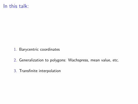
In this talk:

1. Barycentric coordinates

2. Generalization to polygons: Wachspress, mean value, etc.

3. Transfinite interpolation

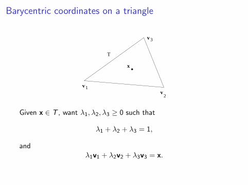
Barycentric coordinates on a triangle

v 3

v 1v

2

T

x

Given x ∈ T , want λ1, λ2, λ3 ≥ 0 such that

λ1 + λ2 + λ3 = 1,

andλ1v1 + λ2v2 + λ3v3 = x.

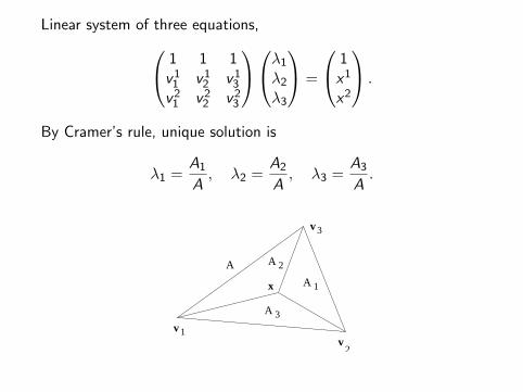
Linear system of three equations, 1 1 1v11 v1

2 v13

v21 v2

2 v23

λ1

λ2

λ3

=

1x1

x2

.

By Cramer’s rule, unique solution is

λ1 =A1

A, λ2 =

A2

A, λ3 =

A3

A.

v 3

v 1v

2

A

A

A

1

2

3

x

A

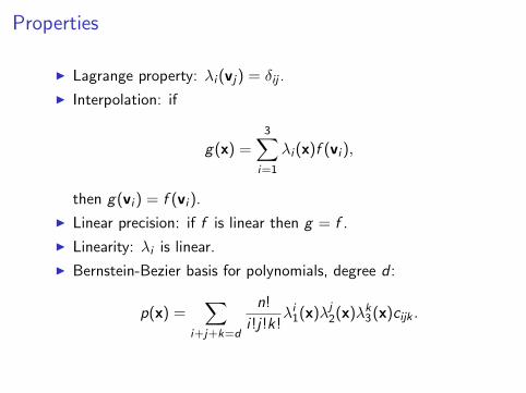
Properties

I Lagrange property: λi (vj) = δij .

I Interpolation: if

g(x) =3∑

i=1

λi (x)f (vi ),

then g(vi ) = f (vi ).

I Linear precision: if f is linear then g = f .

I Linearity: λi is linear.

I Bernstein-Bezier basis for polynomials, degree d :

p(x) =∑

i+j+k=d

n!

i !j!k!λi

1(x)λj2(x)λ

k3(x)cijk .

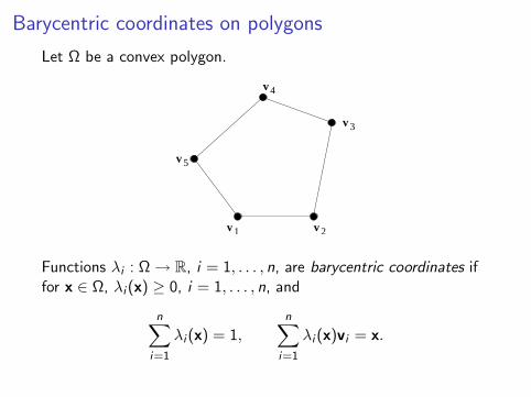
Barycentric coordinates on polygons

Let Ω be a convex polygon.

v v

v

v

v

1 2

3

4

5

Functions λi : Ω → R, i = 1, . . . , n, are barycentric coordinates iffor x ∈ Ω, λi (x) ≥ 0, i = 1, . . . , n, and

n∑i=1

λi (x) = 1,n∑

i=1

λi (x)vi = x.

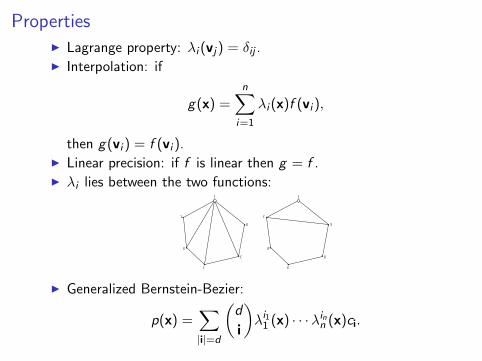
PropertiesI Lagrange property: λi (vj) = δij .I Interpolation: if

g(x) =n∑

i=1

λi (x)f (vi ),

then g(vi ) = f (vi ).I Linear precision: if f is linear then g = f .I λi lies between the two functions:

0

1

0

0

0

00

1

0

0

0

0

I Generalized Bernstein-Bezier:

p(x) =∑|i|=d

(d

i

)λi1

1 (x) · · ·λinn (x)ci.

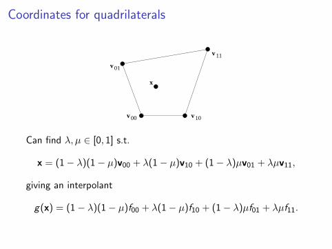
Coordinates for quadrilaterals

v 10v 00

v 01

v 11

x

Can find λ, µ ∈ [0, 1] s.t.

x = (1− λ)(1− µ)v00 + λ(1− µ)v10 + (1− λ)µv01 + λµv11,

giving an interpolant

g(x) = (1− λ)(1− µ)f00 + λ(1− µ)f10 + (1− λ)µf01 + λµf11.

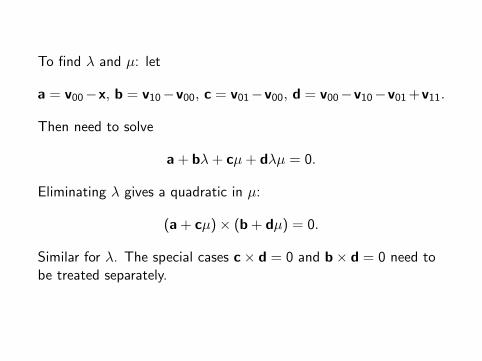
To find λ and µ: let

a = v00−x, b = v10−v00, c = v01−v00, d = v00−v10−v01 +v11.

Then need to solve

a + bλ+ cµ+ dλµ = 0.

Eliminating λ gives a quadratic in µ:

(a + cµ)× (b + dµ) = 0.

Similar for λ. The special cases c× d = 0 and b× d = 0 need tobe treated separately.

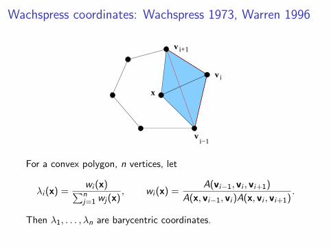
Wachspress coordinates: Wachspress 1973, Warren 1996

vi−1

x

iv

v i+1

For a convex polygon, n vertices, let

λi (x) =wi (x)∑nj=1 wj(x)

, wi (x) =A(vi−1, vi , vi+1)

A(x, vi−1, vi )A(x, vi , vi+1).

Then λ1, . . . , λn are barycentric coordinates.

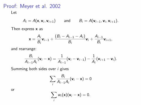
Proof: Meyer et al. 2002Let

Ai = A(x, vi , vi+1) and Bi = A(vi−1, vi , vi+1).

Then express x as

x =Ai

Bivi−1 +

(Bi − Ai−1 − Ai )

Bivi +

Ai−1

Bivi+1,

and rearrange:

Bi

Ai−1Ai(vi − x) =

1

Ai−1(vi − vi−1)−

1

Ai(vi+1 − vi ).

Summing both sides over i gives∑i

Bi

Ai−1Ai(vi − x) = 0

or ∑i

wi (x)(vi − x) = 0.

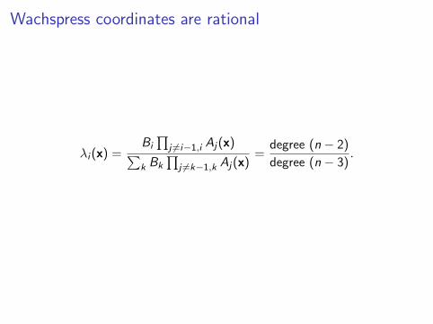
Wachspress coordinates are rational

λi (x) =Bi

∏j 6=i−1,i Aj(x)∑

k Bk∏

j 6=k−1,k Aj(x)=

degree (n − 2)

degree (n − 3).

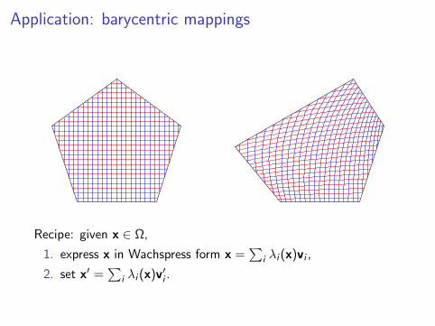
Application: barycentric mappings

Recipe: given x ∈ Ω,

1. express x in Wachspress form x =∑

i λi (x)vi ,

2. set x′ =∑

i λi (x)v′i .

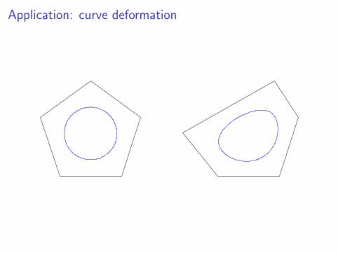
Application: curve deformation

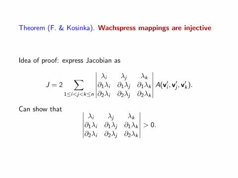
Theorem (F. & Kosinka). Wachspress mappings are injective

Idea of proof: express Jacobian as

J = 2∑

1≤i<j<k≤n

∣∣∣∣∣∣λi λj λk

∂1λi ∂1λj ∂1λk

∂2λi ∂2λj ∂2λk

∣∣∣∣∣∣ A(v′i , v′j , v

′k).

Can show that ∣∣∣∣∣∣λi λj λk

∂1λi ∂1λj ∂1λk

∂2λi ∂2λj ∂2λk

∣∣∣∣∣∣ > 0.

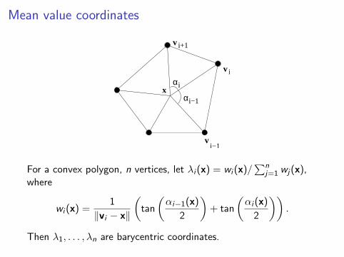
Mean value coordinates

vi−1

x

v i

αi−1

αi

v i+1

For a convex polygon, n vertices, let λi (x) = wi (x)/∑n

j=1 wj(x),where

wi (x) =1

‖vi − x‖

(tan

(αi−1(x)

2

)+ tan

(αi (x)

2

)).

Then λ1, . . . , λn are barycentric coordinates.

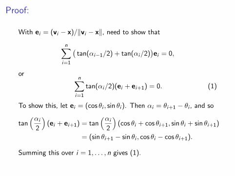
Proof:

With ei = (vi − x)/‖vi − x‖, need to show that

n∑i=1

(tan(αi−1/2) + tan(αi/2)

)ei = 0,

orn∑

i=1

tan(αi/2)(ei + ei+1) = 0. (1)

To show this, let ei = (cos θi , sin θi ). Then αi = θi+1 − θi , and so

tan(αi

2

)(ei + ei+1) = tan

(αi

2

)(cos θi + cos θi+1, sin θi + sin θi+1)

= (sin θi+1 − sin θi , cos θi − cos θi+1).

Summing this over i = 1, . . . , n gives (1).

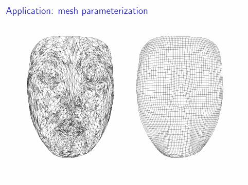
Application: mesh parameterization

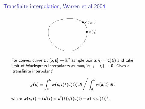
Transfinite interpolation, Warren et al 2004

c ( )t

c t( )i

i+1

For convex curve c : [a, b] → R2 sample points vi = c(ti ) and takelimit of Wachspress interpolants as maxi (ti+1 − ti ) → 0. Gives a‘transfinite interpolant’

g(x) =

∫ b

aw(x, t)f (c(t)) dt

/∫ b

aw(x, t) dt,

where w(x, t) = (c′(t)× c′′(t))/((c(t)− x)× c′(t))2.

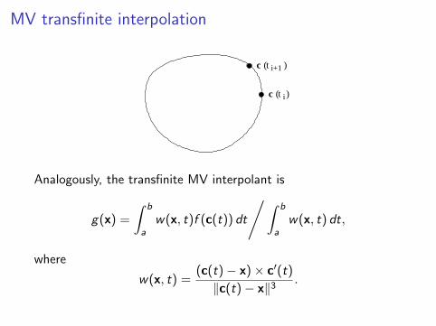
MV transfinite interpolation

c ( )t

c t( )i

i+1

Analogously, the transfinite MV interpolant is

g(x) =

∫ b

aw(x, t)f (c(t)) dt

/∫ b

aw(x, t) dt,

where

w(x, t) =(c(t)− x)× c′(t)

‖c(t)− x‖3.

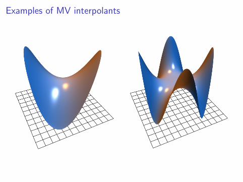
Examples of MV interpolants

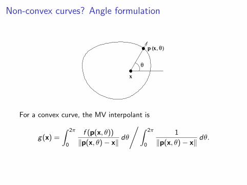
Non-convex curves? Angle formulation

x

( , )x

θ

θp

For a convex curve, the MV interpolant is

g(x) =

∫ 2π

0

f (p(x, θ))

‖p(x, θ)− x‖dθ

/∫ 2π

0

1

‖p(x, θ)− x‖dθ.

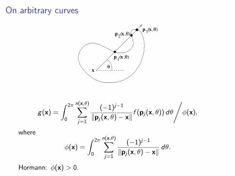
On arbitrary curves

x θ

( , )θx2pp3( , )x θ

p1 x θ( , )

g(x) =

∫ 2π

0

n(x,θ)∑j=1

(−1)j−1

‖pj(x, θ)− x‖f (pj(x, θ)) dθ

/φ(x),

where

φ(x) =

∫ 2π

0

n(x,θ)∑j=1

(−1)j−1

‖pj(x, θ)− x‖dθ.

Hormann: φ(x) > 0.

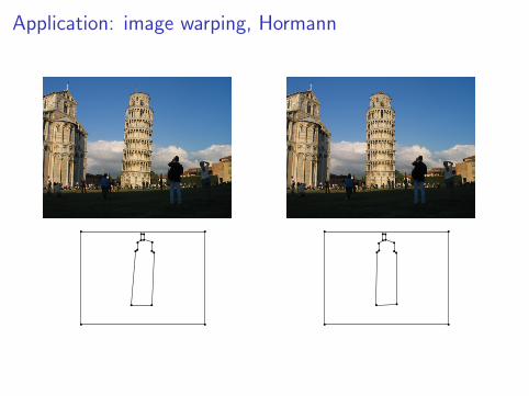
Application: image warping, Hormann

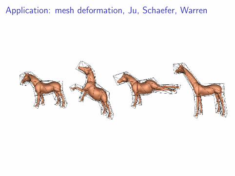
Application: mesh deformation, Ju, Schaefer, Warren

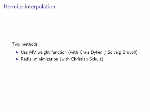
Hermite interpolation

Two methods:

I Use MV weight function (with Chris Dyken / Solveig Bruvoll)

I Radial minimization (with Christian Schulz)

Method 1: weight function

The cubic interpolant p to the data f (0), f ′(0), f (1), f ′(1), can beexpressed as

p(x) = g0(x) + ψ(x)g1(x),

where

g0(x) = (1− x)f (0) + xf (1),

ψ(x) = x(1− x),

g1(x) = (1− x)m0 + xm1,

and

m0 = f ′(0)− f (1) + f (0), m1 = −f ′(1) + f (1)− f (0).

In Rn we interpolate the data f and ∂f∂n on ∂Ω by the function

p(x) = g0(x) + ψ(x)g1(x), x ∈ Ω,

where

g0(x) =

∫S

f (p(x, v))

‖p(x, v)− x‖dv

/φ(x),

ψ(x) = 1

/φ(x),

g1(x) =

∫S

m(p(x, v))

‖p(x, v)− x‖dv

/φ(x),

φ(x) =

∫S

1

‖p(x, v)− x‖dv.

and

m(y) =

(∂f

∂n(y)− ∂g0

∂n(y)

) /∂ψ

∂n(y), y ∈ ∂Ω.

To use this construction we need to find ∂ψ∂n (y) and ∂g0

∂n (y).

TheoremIf d(ME , ∂Ω) > 0 and d(MI , ∂Ω) > 0 and y ∈ ∂Ω then

∂ψ

∂n(y) =

1

Vn−1,

∂g0

∂n(y) =

1

Vn−1

∫H(n)

f (p(y, v))− f (y)

‖p(y, v)− y‖dv,

where Vn−1 is the volume of the unit sphere in Rn−1: V1 = 2,V2 = π, V3 = 4π/3, V4 = π2/2,...

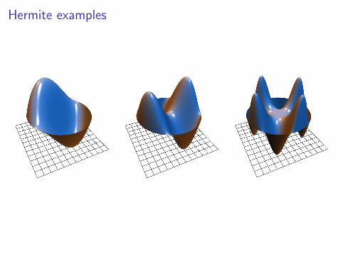
Hermite examples

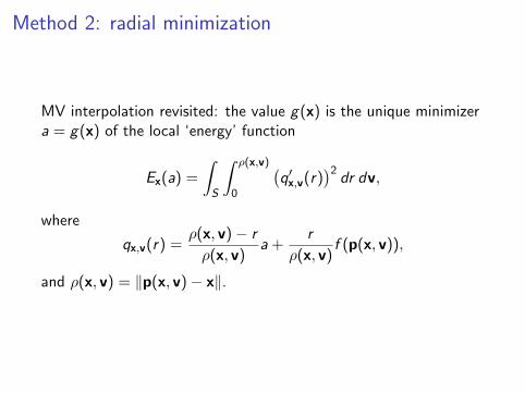
Method 2: radial minimization

MV interpolation revisited: the value g(x) is the unique minimizera = g(x) of the local ‘energy’ function

Ex(a) =

∫S

∫ ρ(x,v)

0

(q′x,v(r)

)2dr dv,

where

qx,v(r) =ρ(x, v)− r

ρ(x, v)a +

r

ρ(x, v)f (p(x, v)),

and ρ(x, v) = ‖p(x, v)− x‖.

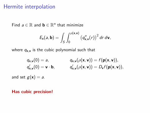
Hermite interpolation

Find a ∈ R and b ∈ Rn that minimize

Ex(a,b) =

∫S

∫ ρ(x,v)

0

(q′′x,v(r)

)2dr dv,

where qx,v is the cubic polynomial such that

qx,v(0) = a, qx,v(ρ(x, v)) = f (p(x, v)),

q′x,v(0) = v · b, q′x,v(ρ(x, v)) = Dvf (p(x, v)),

and set g(x) = a.

Has cubic precision!

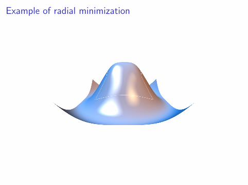
Example of radial minimization

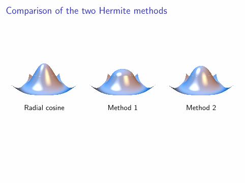
Comparison of the two Hermite methods

Radial cosine Method 1 Method 2