AUTOMATED PROCESS DEPLOYMENT FOR NASTRAN · PDF fileAUTOMATED PROCESS DEPLOYMENT FOR NASTRAN...

2nd ANSA & μETA International Congress June 14-15, 2007 Olympic Convention Center, Porto Carras Grand Resort Hotel, Halkidiki Greece

97

AUTOMATED PROCESS DEPLOYMENT FOR NASTRAN SOL 200 OPTIMIZATION ANALYSIS, USING ANSA/ μETA PACKAGE Georgios Korbetis*, Konstantinos Marmaras BETA CAE Systems S.A., Greece KEYWORDS - optimization, NASTRAN, morphing, task management ABSTRACT - The use of optimization techniques becomes increasingly popular both in the early design stages of the product and during the final testing using the Finite Element Analysis. Furthermore, the computational power now available is sufficient for using optimization on realistic product simulation models. As a result, the increasing complexity of the optimization problem and the subsequent complexity of the optimization software, render essential the use of a tool that organizes the definition of such processes and evaluates the results. Pre-processing for the NASTRAN optimizer is possible through the Task Management functionality of ANSA which provides flexibility, reusability and knowledge transfer. At the same time ANSA’s Morphing Tool provides all the necessary functionality for shape optimization definition and easy coupling with the NASTRAN optimizer, while μETA PostProcessor offers an efficient way to evaluate the results. TECHNICAL PAPER - 1. INTRODUCTION The latest versions of ANSA and μETA support the pre- and post-processing of the optimization problem according to NASTRAN SOL 200. Property and Shape Optimization set up is possible. NASTRAN offers four different methods to define a Shape Optimization problem. These are the Manual Grid Variation Method, the Direct Input of Shapes, the Geometric Boundary Shapes and the Analytic Boundary Shapes. Currently, ANSA supports the Manual Grid Variation method. Following this method, for every grid of the design space, the displacement vectors must be defined. These vectors prescribe the movement of every grid through the optimization loops for a given change in the relative design variable. So for each grid of the design space a DVGRID keyword must be defined which contains the information of the displacement vector and the design variable which drives the grid movement. Even if this is a manual method, the use of ANSA Morphing Tool can automate the definition of DVGRID keywords in a way that all needed data are produced in a single step process. Furthermore, the Morphing Tool ensures that the deformed model’s shape, at any stage of the optimization process, will be smooth. Finally the user can investigate, before running the solver, if an error is possible to come up in the optimization process due to elements quality failure, penetration, etc.. Property optimization is also supported. Currently, ANSA covers all the needed functionality for optimization according to element, material and connectivity properties. Although all keywords concerning NASTRAN SOL 200 are supported in ANSA by functions and cards, the use of the ANSA Task Manager offers a flexible and user-friendly way to define the optimization problem. A case study of finding the optimal shape of a piston rod demonstrates the process set up.


98

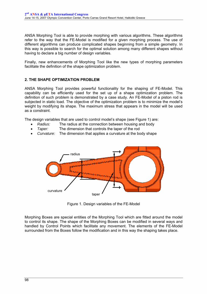
ANSA Morphing Tool is able to provide morphing with various algorithms. These algorithms refer to the way that the FE-Model is modified for a given morphing process. The use of different algorithms can produce complicated shapes beginning from a simple geometry. In this way is possible to search for the optimal solution among many different shapes without having to declare a big number of design variables. Finally, new enhancements of Morphing Tool like the new types of morphing parameters facilitate the definition of the shape optimization problem. 2. THE SHAPE OPTIMIZATION PROBLEM ANSA Morphing Tool provides powerful functionality for the shaping of FE-Model. This capability can be efficiently used for the set up of a shape optimization problem. The definition of such problem is demonstrated by a case study. An FE-Model of a piston rod is subjected in static load. The objective of the optimization problem is to minimize the model’s weight by modifying its shape. The maximum stress that appears in the model will be used as a constraint. The design variables that are used to control model’s shape (see Figure 1) are:

• Radius: The radius at the connection between housing and body • Taper: The dimension that controls the taper of the rod • Curvature: The dimension that applies a curvature at the body shape

Figure 1. Design variables of the FE-Model

Morphing Boxes are special entities of the Morphing Tool which are fitted around the model to control its shape. The shape of the Morphing Boxes can be modified in several ways and handled by Control Points which facilitate any movement. The elements of the FE-Model surrounded from the Boxes follow the modification and in this way the shaping takes place.

taper

radius

curvature


99

Target curve

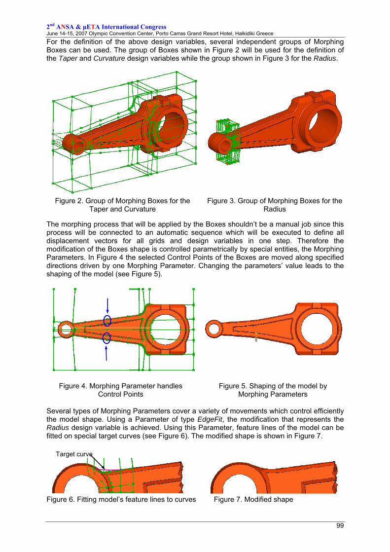
For the definition of the above design variables, several independent groups of Morphing Boxes can be used. The group of Boxes shown in Figure 2 will be used for the definition of the Taper and Curvature design variables while the group shown in Figure 3 for the Radius.

Figure 2. Group of Morphing Boxes for the Taper and Curvature

Figure 3. Group of Morphing Boxes for the Radius

The morphing process that will be applied by the Boxes shouldn’t be a manual job since this process will be connected to an automatic sequence which will be executed to define all displacement vectors for all grids and design variables in one step. Therefore the modification of the Boxes shape is controlled parametrically by special entities, the Morphing Parameters. In Figure 4 the selected Control Points of the Boxes are moved along specified directions driven by one Morphing Parameter. Changing the parameters’ value leads to the shaping of the model (see Figure 5).

Figure 4. Morphing Parameter handles Control Points

Figure 5. Shaping of the model by Morphing Parameters

Several types of Morphing Parameters cover a variety of movements which control efficiently the model shape. Using a Parameter of type EdgeFit, the modification that represents the Radius design variable is achieved. Using this Parameter, feature lines of the model can be fitted on special target curves (see Figure 6). The modified shape is shown in Figure 7.

Figure 6. Fitting model’s feature lines to curves Figure 7. Modified shape


100

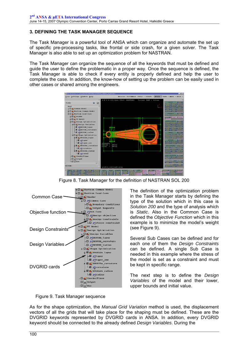
3. DEFINING THE TASK MANAGER SEQUENCE The Task Manager is a powerful tool of ANSA which can organize and automate the set up of specific pre-processing tasks, like frontal or side crash, for a given solver. The Task Manager is also able to set up an optimization problem for NASTRAN. The Task Manager can organize the sequence of all the keywords that must be defined and guide the user to define the problematic in a proper way. Once the sequence is defined, the Task Manager is able to check if every entity is properly defined and help the user to complete the case. In addition, the know-how of setting up the problem can be easily used in other cases or shared among the engineers.

Figure 8. Task Manager for the definition of NASTRAN SOL 200

The definition of the optimization problem in the Task Manager starts by defining the type of the solution which in this case is Solution 200 and the type of analysis which is Static. Also in the Common Case is defined the Objective Function which in this example is to minimize the model’s weight (see Figure 9). Several Sub Cases can be defined and for each one of them the Design Constraints can be defined. A single Sub Case is needed in this example where the stress of the model is set as a constraint and must be kept in specific range. The next step is to define the Design Variables of the model and their lower, upper bounds and initial value.

Figure 9. Task Manager sequence As for the shape optimization, the Manual Grid Variation method is used, the displacement vectors of all the grids that will take place for the shaping must be defined. These are the DVGRID keywords represented by DVGRID cards in ANSA. In addition, every DVGRID keyword should be connected to the already defined Design Variables. During the

Common Case

Objective function

Design Constraints

Design Variables

DVGRID cards


101

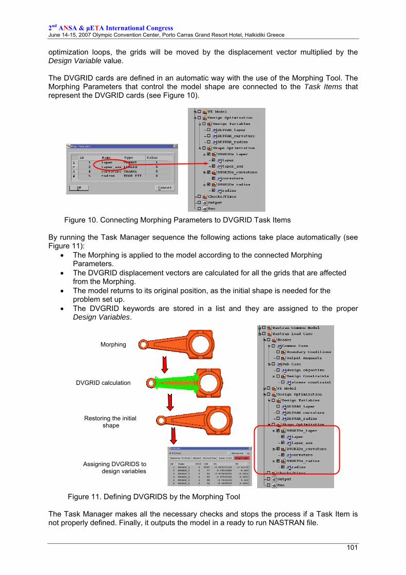
optimization loops, the grids will be moved by the displacement vector multiplied by the Design Variable value. The DVGRID cards are defined in an automatic way with the use of the Morphing Tool. The Morphing Parameters that control the model shape are connected to the Task Items that represent the DVGRID cards (see Figure 10).

Figure 10. Connecting Morphing Parameters to DVGRID Task Items

By running the Task Manager sequence the following actions take place automatically (see Figure 11):

• The Morphing is applied to the model according to the connected Morphing Parameters.

• The DVGRID displacement vectors are calculated for all the grids that are affected from the Morphing.

• The model returns to its original position, as the initial shape is needed for the problem set up.

• The DVGRID keywords are stored in a list and they are assigned to the proper Design Variables.

Figure 11. Defining DVGRIDS by the Morphing Tool

The Task Manager makes all the necessary checks and stops the process if a Task Item is not properly defined. Finally, it outputs the model in a ready to run NASTRAN file.

Morphing

DVGRID calculation

Restoring the initial shape

Assigning DVGRIDS to design variables


102

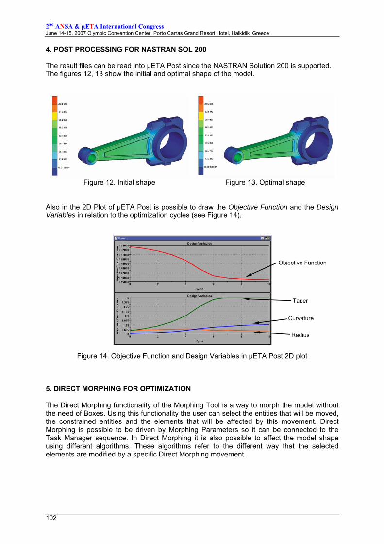
4. POST PROCESSING FOR NASTRAN SOL 200 The result files can be read into μETA Post since the NASTRAN Solution 200 is supported. The figures 12, 13 show the initial and optimal shape of the model.

Figure 12. Initial shape Figure 13. Optimal shape Also in the 2D Plot of μETA Post is possible to draw the Objective Function and the Design Variables in relation to the optimization cycles (see Figure 14).

Figure 14. Objective Function and Design Variables in μETA Post 2D plot 5. DIRECT MORPHING FOR OPTIMIZATION The Direct Morphing functionality of the Morphing Tool is a way to morph the model without the need of Boxes. Using this functionality the user can select the entities that will be moved, the constrained entities and the elements that will be affected by this movement. Direct Morphing is possible to be driven by Morphing Parameters so it can be connected to the Task Manager sequence. In Direct Morphing it is also possible to affect the model shape using different algorithms. These algorithms refer to the different way that the selected elements are modified by a specific Direct Morphing movement.

Taper

Objective Function

Curvature

Radius


103

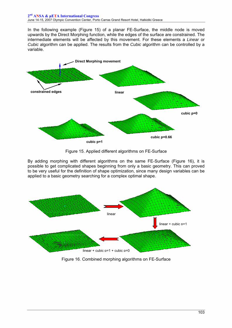
In the following example (Figure 15) of a planar FE-Surface, the middle node is moved upwards by the Direct Morphing function, while the edges of the surface are constrained. The intermediate elements will be affected by this movement. For these elements a Linear or Cubic algorithm can be applied. The results from the Cubic algorithm can be controlled by a variable.

Figure 15. Applied different algorithms on FE-Surface By adding morphing with different algorithms on the same FE-Surface (Figure 16), it is possible to get complicated shapes beginning from only a basic geometry. This can proved to be very useful for the definition of shape optimization, since many design variables can be applied to a basic geometry searching for a complex optimal shape.

Figure 16. Combined morphing algorithms on FE-Surface

linear

Direct Morphing movement

constrained edges

cubic p=0

cubic p=1 cubic p=0.66

linear

linear + cubic p=1

linear + cubic p=1 + cubic p=0


104

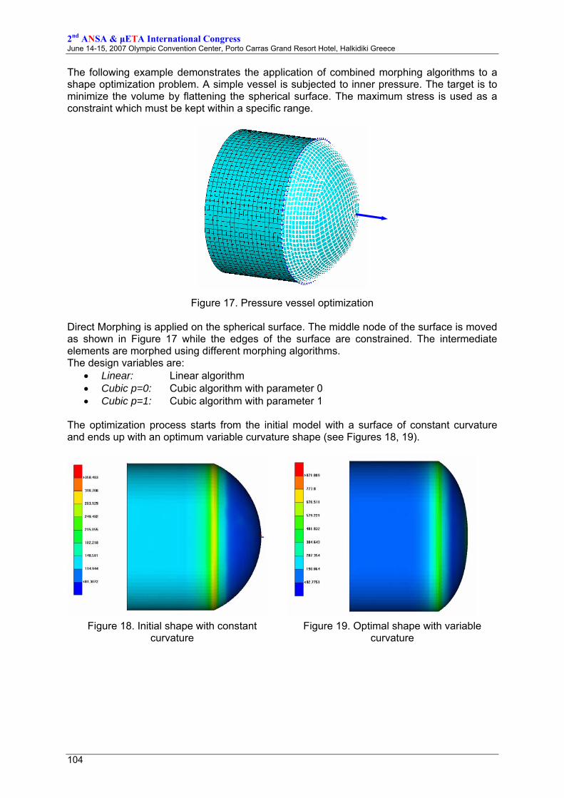
The following example demonstrates the application of combined morphing algorithms to a shape optimization problem. A simple vessel is subjected to inner pressure. The target is to minimize the volume by flattening the spherical surface. The maximum stress is used as a constraint which must be kept within a specific range.

Figure 17. Pressure vessel optimization Direct Morphing is applied on the spherical surface. The middle node of the surface is moved as shown in Figure 17 while the edges of the surface are constrained. The intermediate elements are morphed using different morphing algorithms. The design variables are:

• Linear: Linear algorithm • Cubic p=0: Cubic algorithm with parameter 0 • Cubic p=1: Cubic algorithm with parameter 1

The optimization process starts from the initial model with a surface of constant curvature and ends up with an optimum variable curvature shape (see Figures 18, 19).

Figure 18. Initial shape with constant

curvature Figure 19. Optimal shape with variable

curvature


105

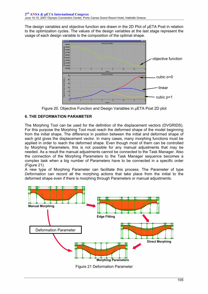
The design variables and objective function are drawn in the 2D Plot of μETA Post in relation to the optimization cycles. The values of the design variables at the last stage represent the usage of each design variable to the composition of the optimal shape.

Figure 20. Objective Function and Design Variables in μETA Post 2D plot

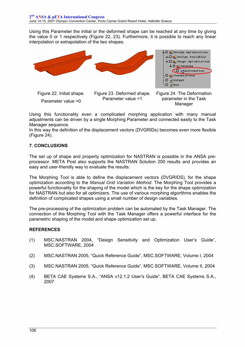
6. THE DEFORMATION PARAMETER The Morphing Tool can be used for the definition of the displacement vectors (DVGRIDS). For this purpose the Morphing Tool must reach the deformed shape of the model beginning from the initial shape. The difference in position between the initial and deformed shape of each grid gives the displacement vector. In many cases, many morphing functions must be applied in order to reach the deformed shape. Even though most of them can be controlled by Morphing Parameters, this is not possible for any manual adjustments that may be needed. As a result the manual adjustments cannot be connected to the Task Manager. Also the connection of the Morphing Parameters to the Task Manager sequence becomes a complex task when a big number of Parameters have to be connected in a specific order (Figure 21). A new type of Morphing Parameter can facilitate this process. The Parameter of type Deformation can record all the morphing actions that take place from the initial to the deformed shape even if there is morphing through Parameters or manual adjustments.

Figure 21 Deformation Parameter

objective function

cubic p=0

cubic p=1

linear

Manual Morphing

Edge Fitting

Morphing Parameters

Deformation Parameter

Direct Morphing


106

Using this Parameter the initial or the deformed shape can be reached at any time by giving the value 0 or 1 respectively (Figure 22, 23). Furthermore, it is possible to reach any linear interpolation or extrapolation of the two shapes.

Figure 22. Initial shape.

Parameter value =0

Figure 23. Deformed shape. Parameter value =1

Figure 24. The Deformation parameter in the Task

Manager Using this functionality even a complicated morphing application with many manual adjustments can be driven by a single Morphing Parameter and connected easily to the Task Manager sequence. In this way the definition of the displacement vectors (DVGRIDs) becomes even more flexible (Figure 24). 7. CONCLUSIONS The set up of shape and property optimization for NASTRAN is possible in the ANSA pre-processor. ΜETA Post also supports the NASTRAN Solution 200 results and provides an easy and user-friendly way to evaluate the results. The Morphing Tool is able to define the displacement vectors (DVGRIDS), for the shape optimization according to the Manual Grid Variation Method. The Morphing Tool provides a powerful functionality for the shaping of the model which is the key for the shape optimization for NASTRAN but also for all optimizers. The use of various morphing algorithms enables the definition of complicated shapes using a small number of design variables. The pre-processing of the optimization problem can be automated by the Task Manager. The connection of the Morphing Tool with the Task Manager offers a powerful interface for the parametric shaping of the model and shape optimization set up. REFERENCES (1) MSC.NASTRAN 2004, “Design Sensitivity and Optimization User’s Guide”,

MSC.SOFTWARE, 2004 (2) MSC.NASTRAN 2005, “Quick Reference Guide”, MSC.SOFTWARE, Volume I, 2004 (3) MSC.NASTRAN 2005, “Quick Reference Guide”, MSC.SOFTWARE, Volume II, 2004 (4) BETA CAE Systems S.A., “ANSA v12.1.2 User’s Guide”, BETA CAE Systems S.A.,

2007

AUTOMATED PROCESS DEPLOYMENT FOR NASTRAN · PDF fileAUTOMATED PROCESS DEPLOYMENT FOR NASTRAN...

Documents

Transcript of AUTOMATED PROCESS DEPLOYMENT FOR NASTRAN · PDF fileAUTOMATED PROCESS DEPLOYMENT FOR NASTRAN...