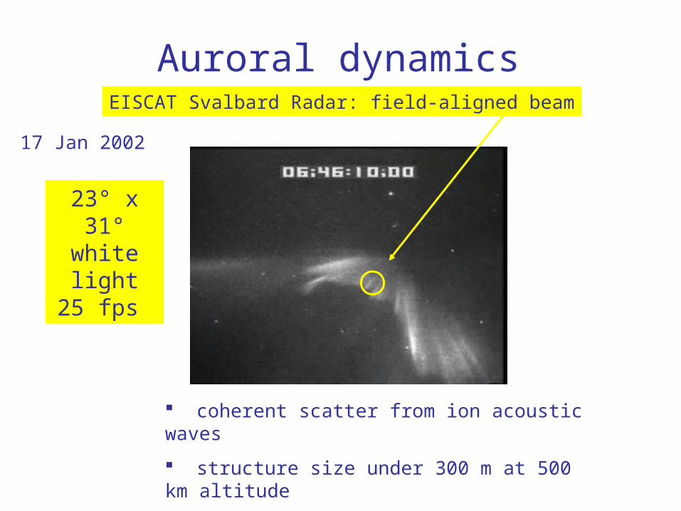
Auroral dynamicsEISCAT Svalbard Radar: field-aligned beam

complicated spatial structure (<1 km)

fast temporal variations (<1 second)

17 Jan 2002

23° x 31°white light

25 fps

coherent scatter from ion acoustic waves

structure size under 300 m at 500 km altitude

varying on 0.2 second time scale

North

West

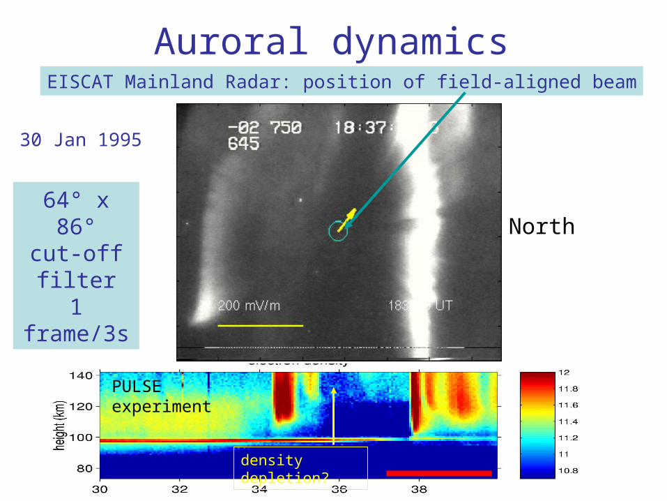
Auroral dynamicsEISCAT Mainland Radar: position of field-aligned beam

64° x 86°cut-off filter1 frame/3s

30 Jan 1995

dynamic range problems

geometry of 3 D multiple structures seen in 2 D

white light or cut-off filterdensity depletion?

PULSE experiment

Auroral fine structure

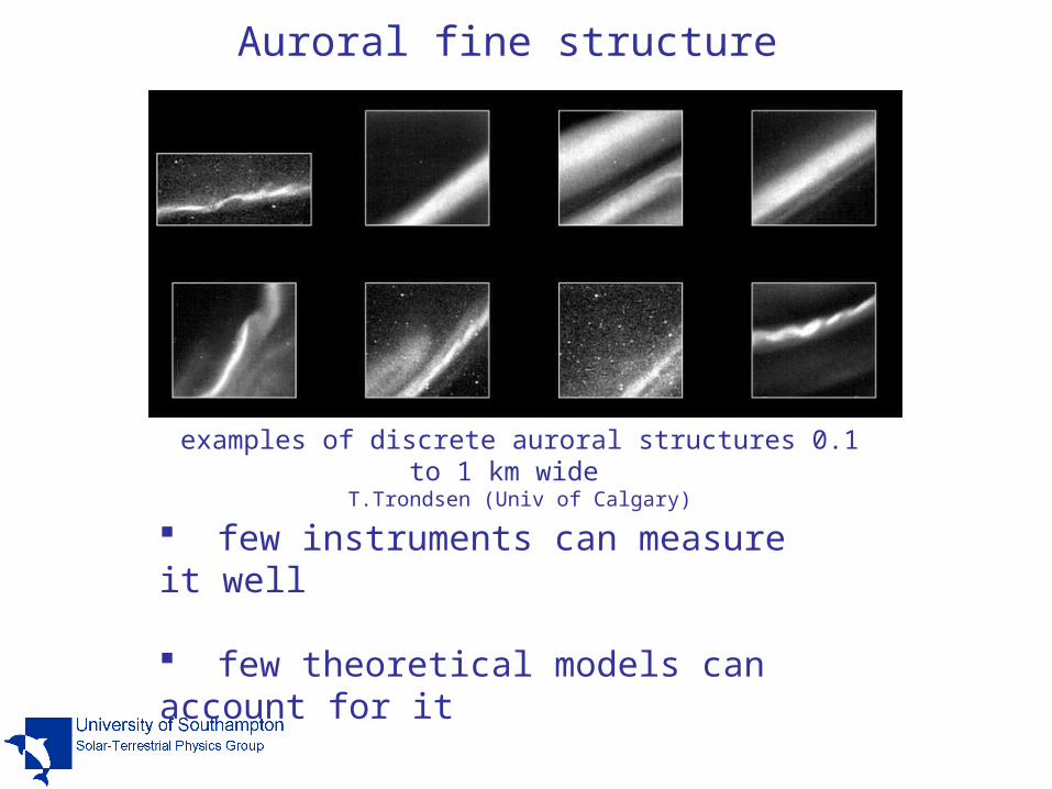
examples of discrete auroral structures 0.1 to 1 km wide T.Trondsen (Univ of Calgary)

few instruments can measure it well

few theoretical models can account for it

What are the unsolved problems?

The big one: how are particles accelerated?

Is the filamentary structure important, especially for field-aligned currents?

How well do theories account for the dynamics observed?

Are rays just curls seen from the side?

etc.

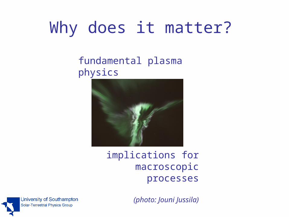
Why does it matter?

fundamental plasma physics

implications for macroscopic processes

(photo: Jouni Jussila)

Observationssome properties of discrete aurora

• multiple (parallel) curtains or filaments (< 1km)

• dynamic rayed aurora

• large amplitude spiky electric fields in the acceleration region

• time scales between fractions of seconds and minutes

• strong velocity shear near discrete aurora

• major portion of current carried by low energy electrons

Our approach to the problem- fit measurements to theory

1. Optical and radar observations

2. Modelling (1D, 2D and 3D)

3. New ASK instrument to measure

plasma flows at high resolution,

and low energy precipitation

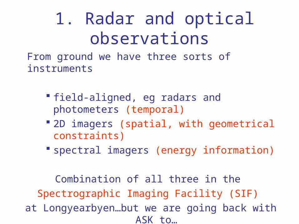
1. Radar and optical observations

From ground we have three sorts of instruments

field-aligned, eg radars and photometers (temporal) 2D imagers (spatial, with geometrical constraints) spectral imagers (energy information)

Combination of all three in the

Spectrographic Imaging Facility (SIF)

at Longyearbyen…but we are going back with ASK to…

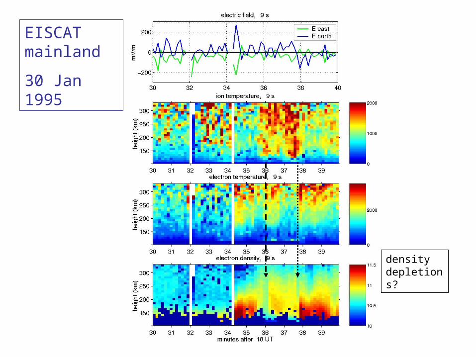
EISCAT mainland

30 Jan 1995

density depletions?

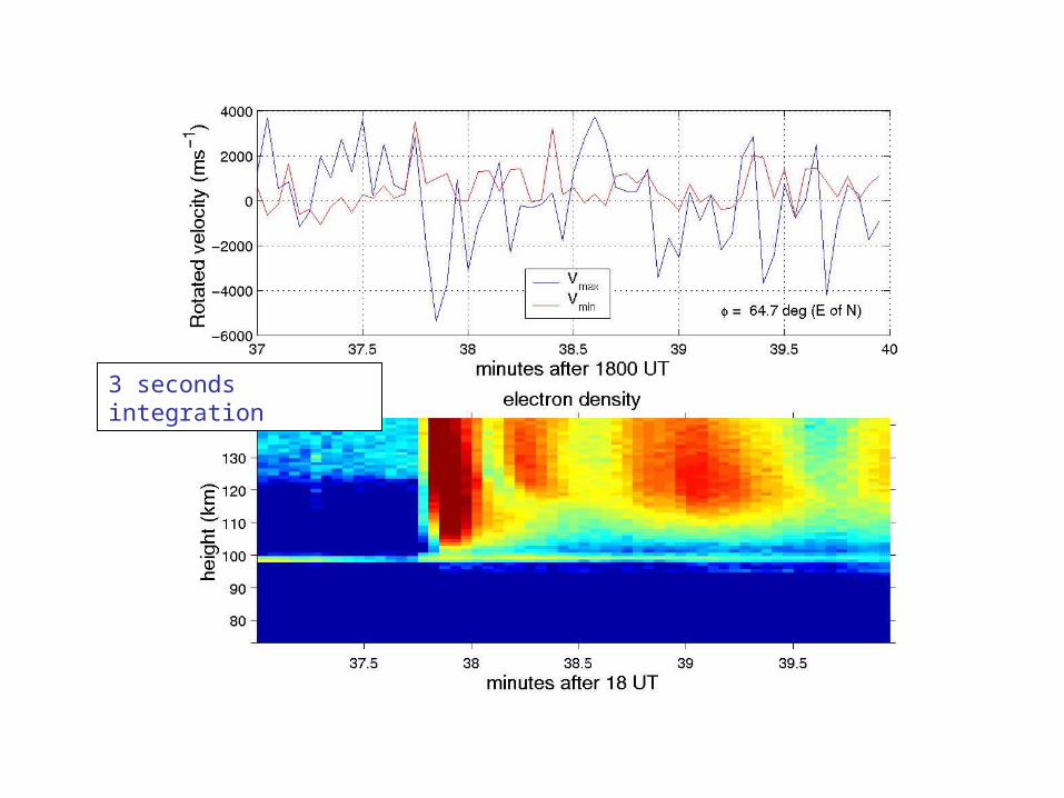
3 seconds integration

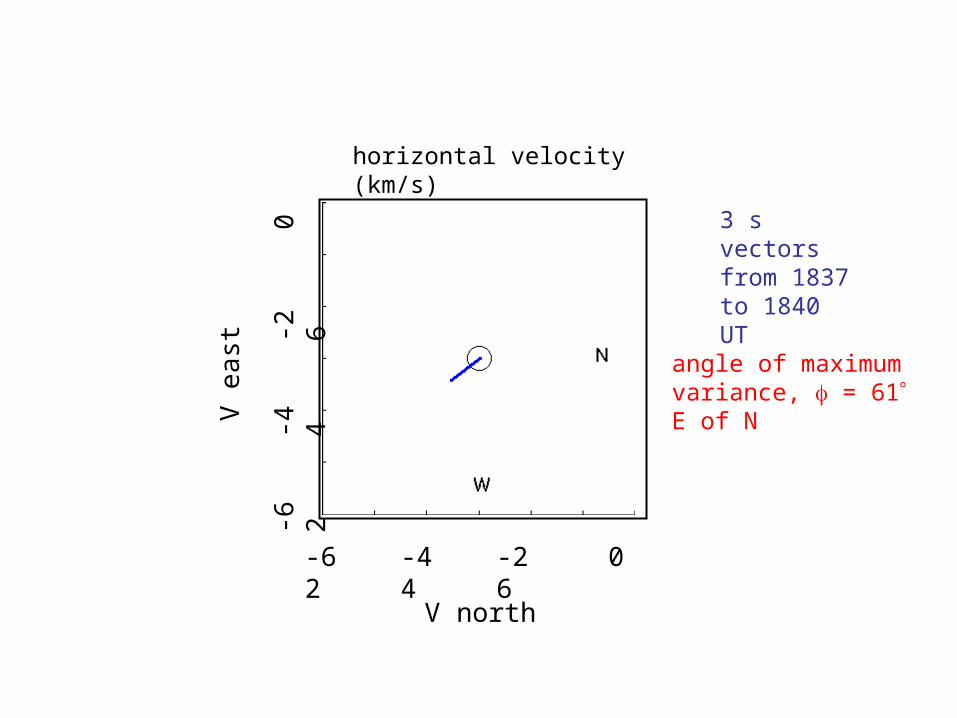
horizontal velocity (km/s)

-6 -4 -2 0 2 4 6

-6

-4

-2

0

2

4

6

V north

V e

ast

3 s vectors from 1837 to 1840 UT

angle of maximum variance, = 61 E of N

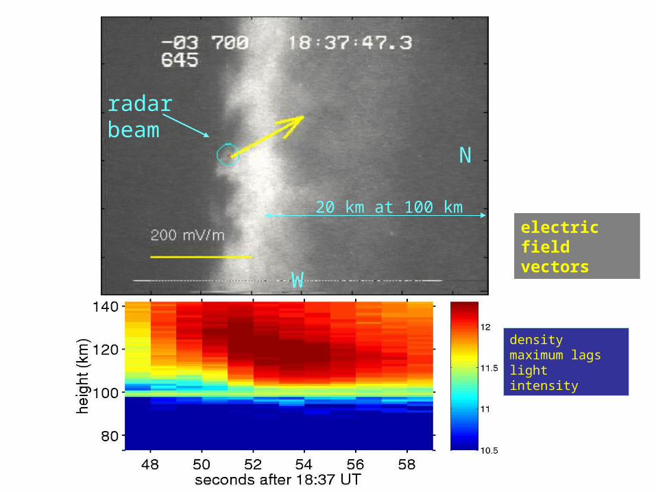
density maximum lags light intensity

N

W

radar beam

20 km at 100 kmelectric field vectors

25 km

10 km

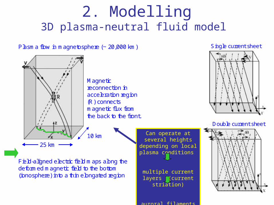
Plasma flow in magnetosphere (~ 20,000 km)

Magneticreconnection inacceleration region(R) connectsmagnetic flux fromthe back to the front.

Field-aligned electric field maps along thedeformed magnetic field to the bottom(ionosphere) into a thin elongated region

3-D plasma-neutral fluid model2. Modelling

3D plasma-neutral fluid model

Single current sheet

Double current sheet

Can operate at several heights depending on

local plasma conditions

multiple current layers (current striation)

auroral filaments

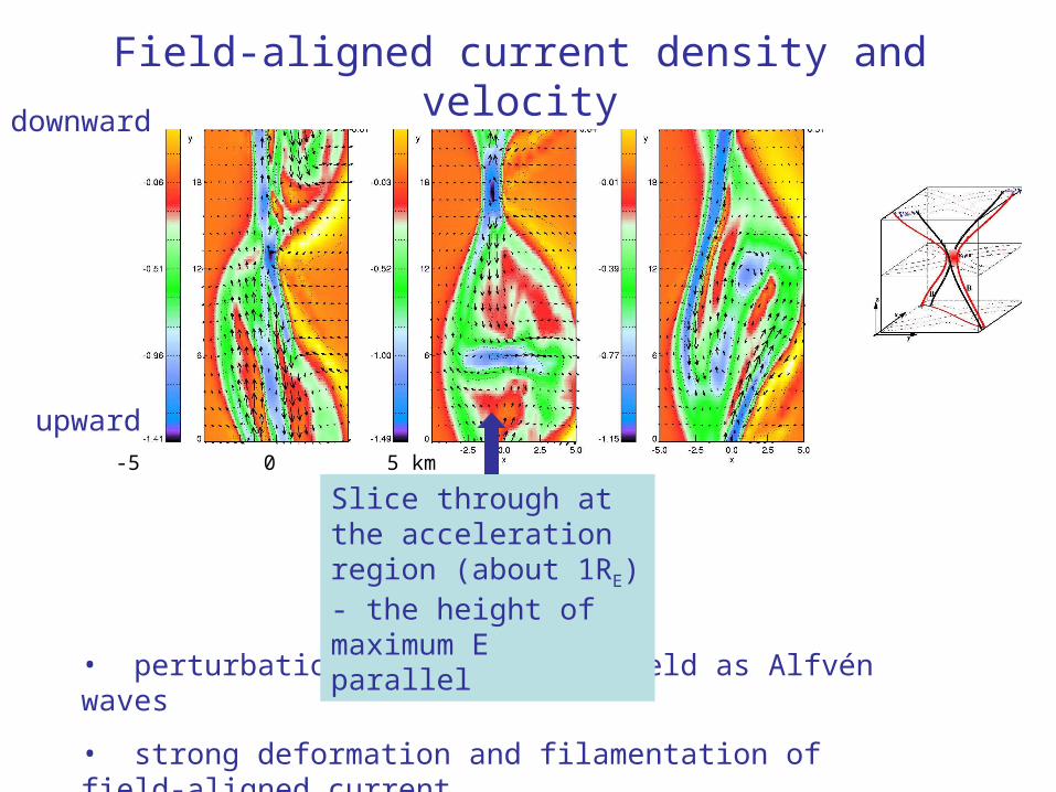
• perturbation travels along field as Alfvén waves

• strong deformation and filamentation of field-aligned current

-5 0 5 km

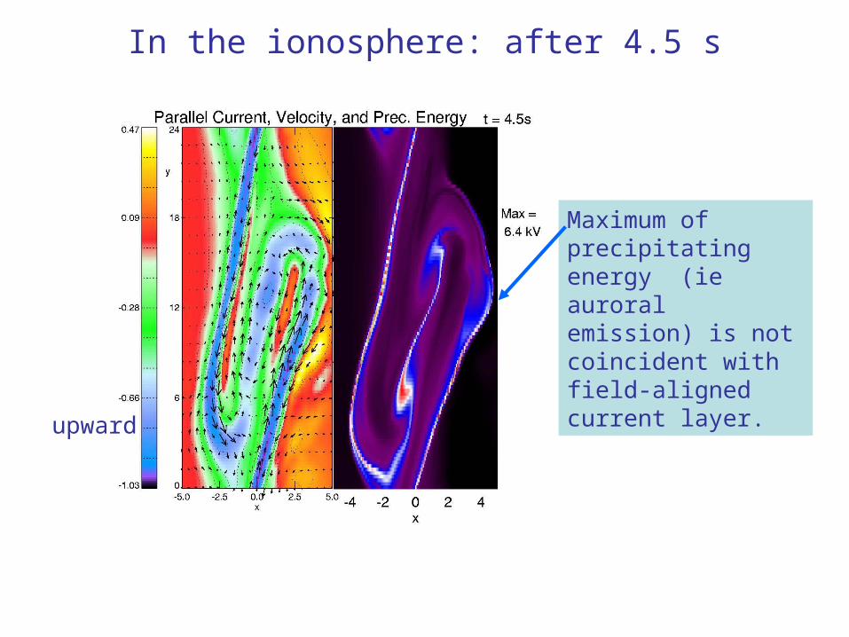
Slice through at the acceleration region (about 1RE) - the height of maximum E parallel

Field-aligned current density and velocity

upward

downward

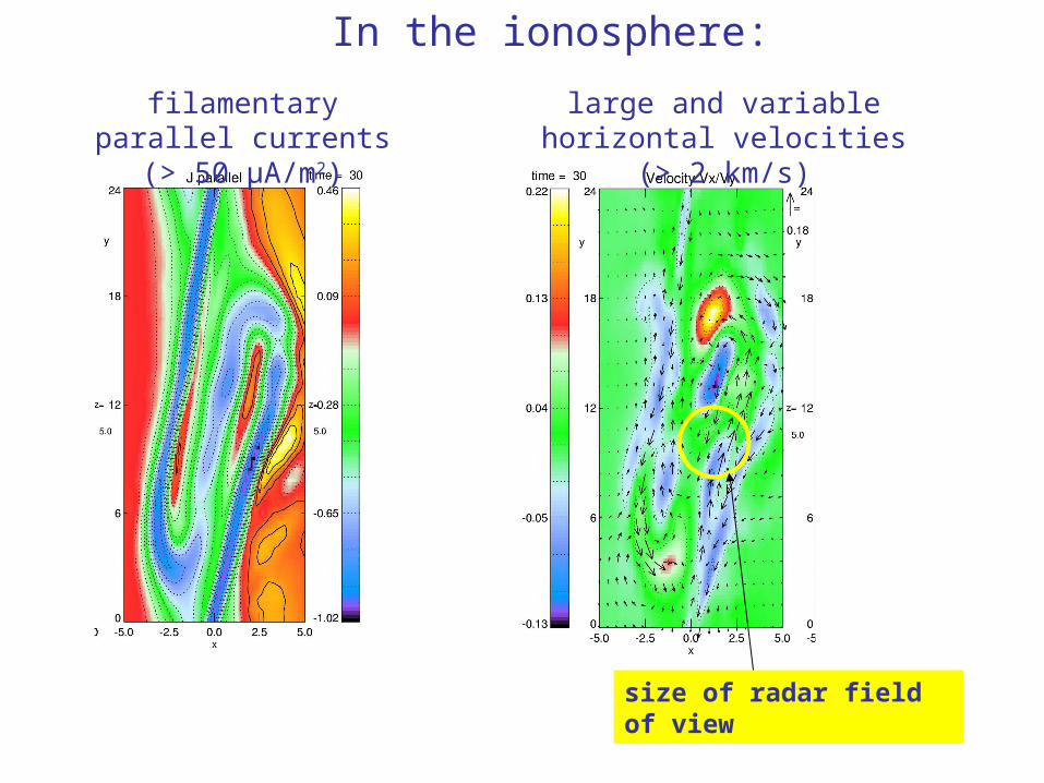
In the ionosphere:

size of radar field of view

large and variable horizontal velocities (> 2 km/s)

filamentary parallel currents (> 50 μA/m2)

upward

In the ionosphere: after 4.5 s

Maximum of precipitating energy (ie auroral emission) is not coincident with field-aligned current layer.

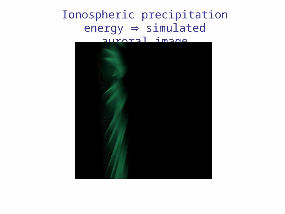
Ionospheric precipitation energy simulated auroral image

How to generate large velocities

100 nT + average plasma density (1-2 km/s)

400 nT or low density plasma (4-8 km/s)

only very fast time variation can generate high speed flows

To image aurora in the magnetic zenith in forbidden ion line and directly observe plasma drifts, with sub-km and sub-sec resolution. Concurrent imaging in other lines characterises the production of the

metastable ions.

3. The ASK concept

ASK stands for the ”Auroral Structure and Kinetics”

So....

Physics summary how to generate auroral structure- top to bottom

structure and processes at magnetospheric boundariessolar wind dynamic pressure changes, magnetic reconnection, Kelvin Helmholtz instabilities,

diffusion by micro turbulence

physical mechanism for transport of informationfield-aligned currents and Alfvén waves, fast waves or beams of particles

field-aligned currents – magnetic field geometry alteredIf processes lead to a violation of frozen-in condition magnetic field lines have no identity

transport of information not linear physical processes in the inner magnetosphere could alter the magnetic topology, violate the

frozen-in condition and generate structures in addition to those of the source at the magnetospheric boundary

effect of ionosphere changes in ionospheric conductivity from particle precipitation will have a significant influence on

magnetosphere-ionosphere coupling