Atomic Structure and the Fine structure constant α
30
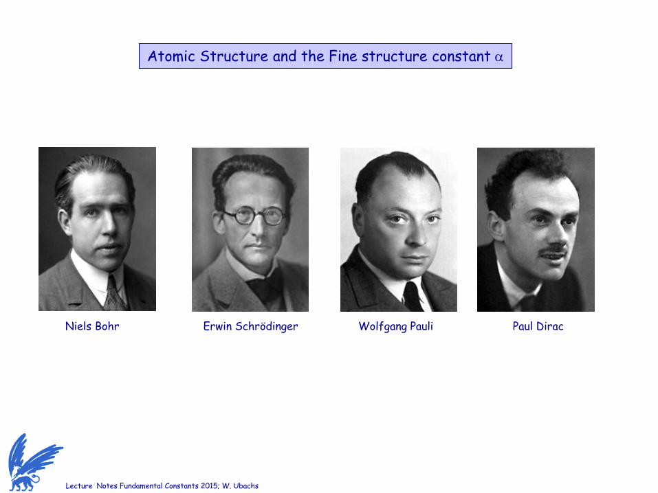
Lecture Notes Fundamental Constants 2015; W. Ubachs Atomic Structure and the Fine structure constant α Niels Bohr Erwin Schrödinger Wolfgang Pauli Paul Dirac
Transcript of Atomic Structure and the Fine structure constant α
Lecture Notes Fundamental Constants 2015; W. Ubachs
Atomic Structure and the Fine structure constant α
Niels Bohr Erwin Schrödinger Wolfgang Pauli Paul Dirac
Lecture Notes Fundamental Constants 2015; W. Ubachs
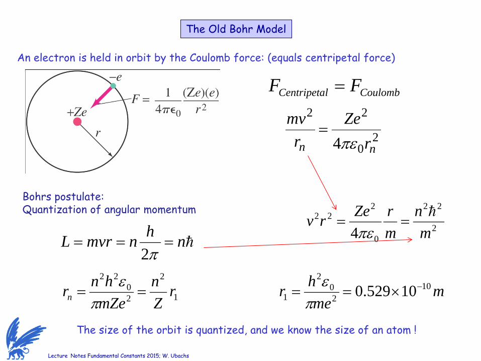
The Old Bohr Model
An electron is held in orbit by the Coulomb force: (equals centripetal force)
20
22
4 nn rZe
rmv
πε=
The size of the orbit is quantized, and we know the size of an atom !
CoulomblCentripeta FF =
nhnmvrL ===π2
Bohrs postulate: Quantization of angular momentum
2
22
0
222
4 mn
mrZerv
==πε
1
2
20
22
rZn
mZehnrn ==
πε m
mehr 10
20
2
1 10529.0 −×==π
ε
Lecture Notes Fundamental Constants 2015; W. Ubachs
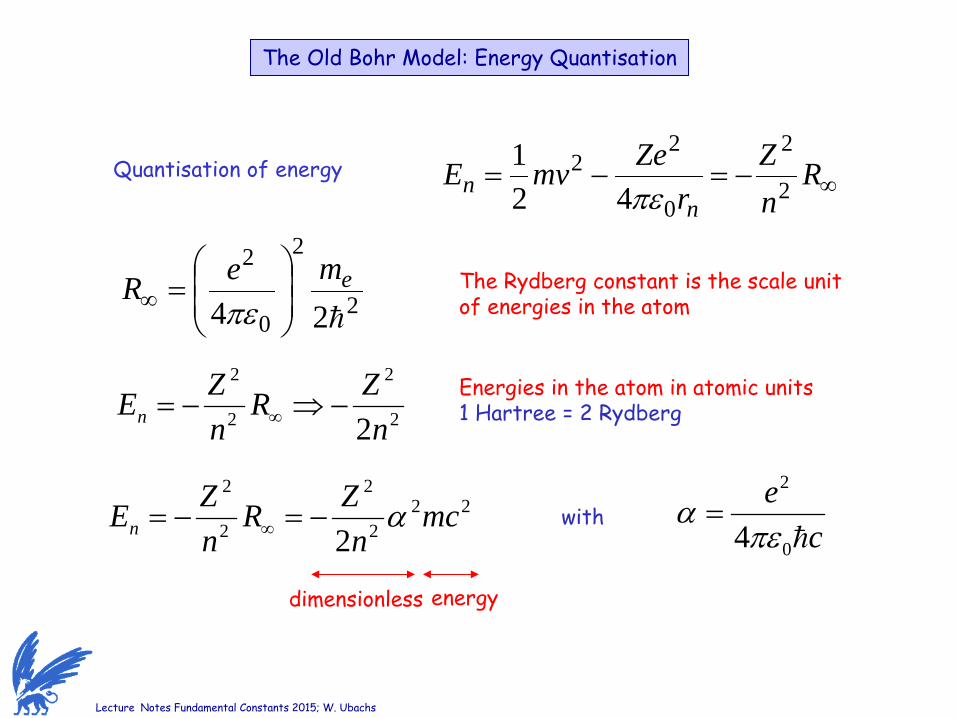
The Old Bohr Model: Energy Quantisation
∞−=−= RnZ
rZemvE
nn 2
2
0
22
421
πεQuantisation of energy
2
2
0
2
24
emeR
=∞ πε
The Rydberg constant is the scale unit of energies in the atom
2
2
2
2
2nZR
nZEn −⇒−= ∞
Energies in the atom in atomic units 1 Hartree = 2 Rydberg
222
2
2
2
2mc
nZR
nZEn α−=−= ∞ c
e0
2
4πεα =with
dimensionless energy
Lecture Notes Fundamental Constants 2015; W. Ubachs
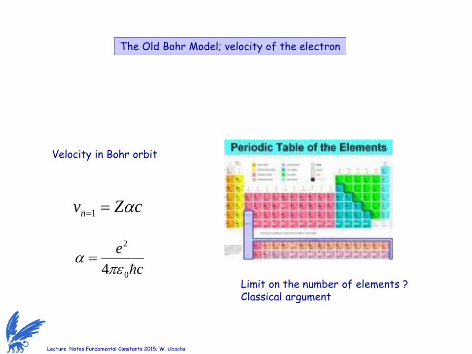
The Old Bohr Model; velocity of the electron
ce0
2
4πεα =
cZvn α==1
Limit on the number of elements ? Classical argument
Velocity in Bohr orbit
Lecture Notes Fundamental Constants 2015; W. Ubachs
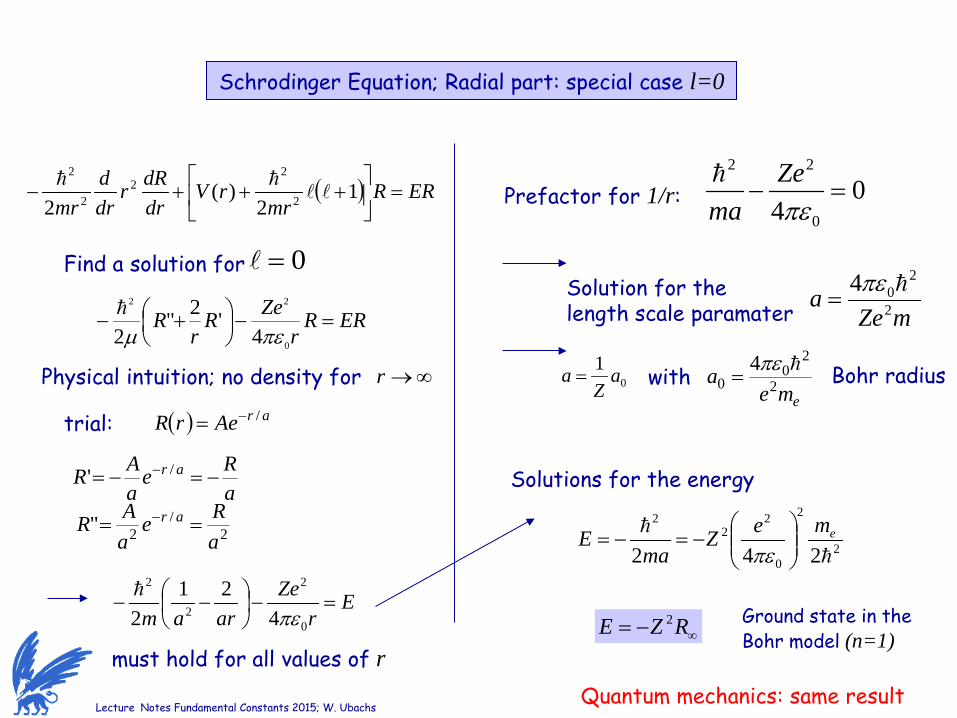
Schrodinger Equation; Radial part: special case l=0
( ) ERRmr
rVdrdRr
drd
mr=
+++− 1
2)(
2 2
22
2
2
Find a solution for 0=
ERRr
ZeRr
R =−
+−
0
22
4'2"
2 πεµ
Physical intuition; no density for ∞→r
trial: ( ) arAerR /−=
aRe
aAR ar −=−= − /'
2/
2"aRe
aAR ar == −
Er
Zearam
=−
−−
0
2
2
2
421
2 πε
must hold for all values of r
04 0
22
=−πεZe
ma
Prefactor for 1/r:
mZea 2
204 πε
=Solution for the length scale paramater
01 aZ
a = with eme
a 2
20
04 πε
= Bohr radius
Solutions for the energy
2
2
0
22
2
242
emeZma
E
−=−=
πε
∞−= RZE 2 Ground state in the Bohr model (n=1)
Quantum mechanics: same result
Lecture Notes Fundamental Constants 2015; W. Ubachs
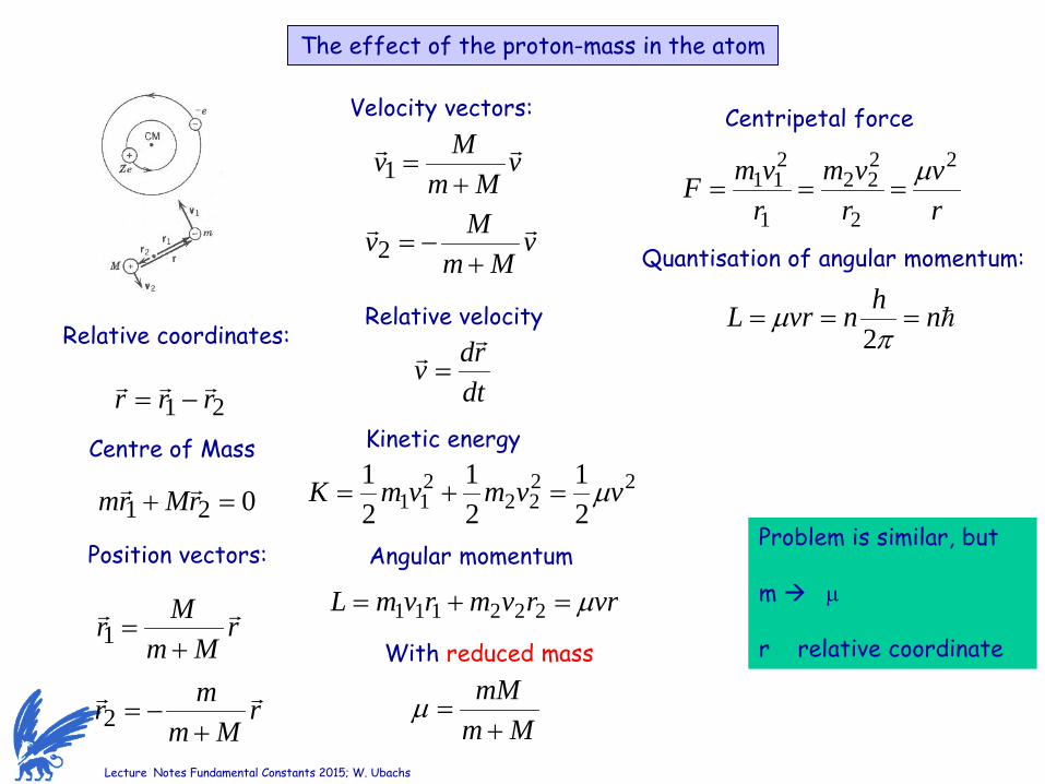
The effect of the proton-mass in the atom
Relative coordinates:
21 rrr −=
Centre of Mass
021 =+ rMrm
Position vectors:
rMm
Mr
+=1
rMm
mr
+−=2
Velocity vectors:
vMm
Mv
+=1
vMm
Mv
+−=2
Relative velocity
dtrdv
=
Kinetic energy
2222
211 2
121
21 vvmvmK µ=+=
With reduced mass
MmmM+
=µ
Angular momentum
vrrvmrvmL µ=+= 222111
Centripetal force
rv
rvm
rvmF
2
2
222
1
211 µ
===
Quantisation of angular momentum:
nhnvrL ===π
µ2
Problem is similar, but m µ r relative coordinate
Lecture Notes Fundamental Constants 2015; W. Ubachs
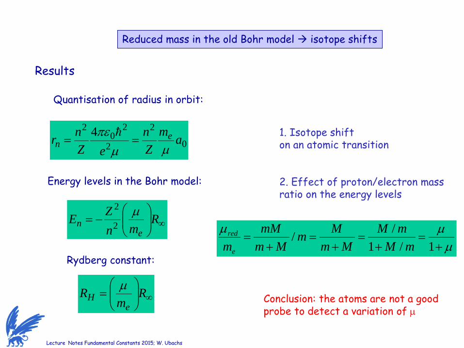
Reduced mass in the old Bohr model isotope shifts
Quantisation of radius in orbit:
0
2
2
20
2 4 amZn
eZnr e
n µµπε
==
Energy levels in the Bohr model:
∞
−= R
mnZE
en
µ2
2
Results
Rydberg constant:
∞
= R
mR
eH
µ
1. Isotope shift on an atomic transition 2. Effect of proton/electron mass ratio on the energy levels
µµµ+
=+
=+
=+
=1/1
//mM
mMMm
MmMm
mMme
red
Conclusion: the atoms are not a good probe to detect a variation of µ
Lecture Notes Fundamental Constants 2015; W. Ubachs
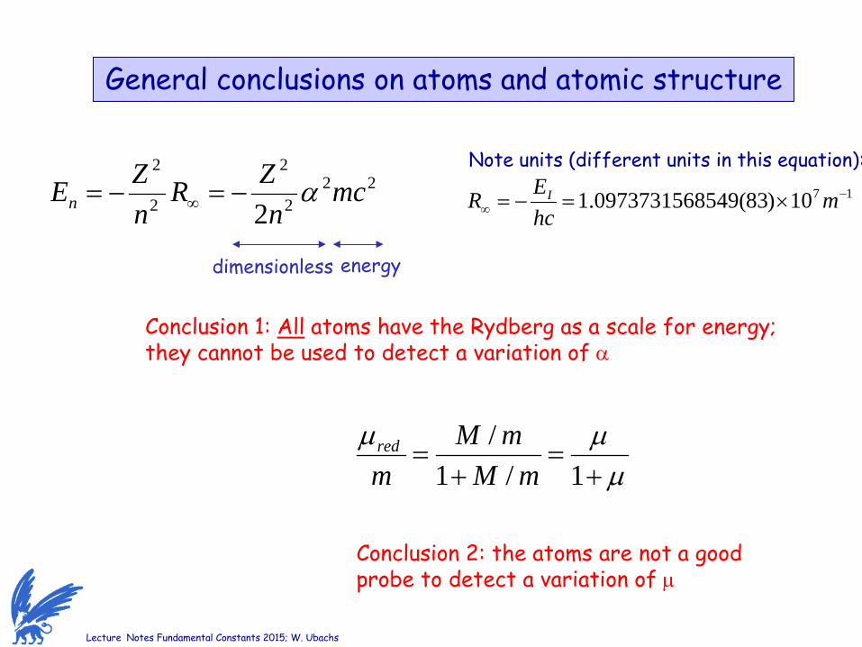
General conclusions on atoms and atomic structure
Conclusion 2: the atoms are not a good probe to detect a variation of µ
222
2
2
2
2mc
nZR
nZEn α−=−= ∞
dimensionless energy
Conclusion 1: All atoms have the Rydberg as a scale for energy; they cannot be used to detect a variation of α
µµµ+
=+
=1/1
/mM
mMmred
Note units (different units in this equation): 1710)83(5490973731568.1 −
∞ ×=−= mhcER I
Lecture Notes Fundamental Constants 2015; W. Ubachs
Relativistic effects in atoms
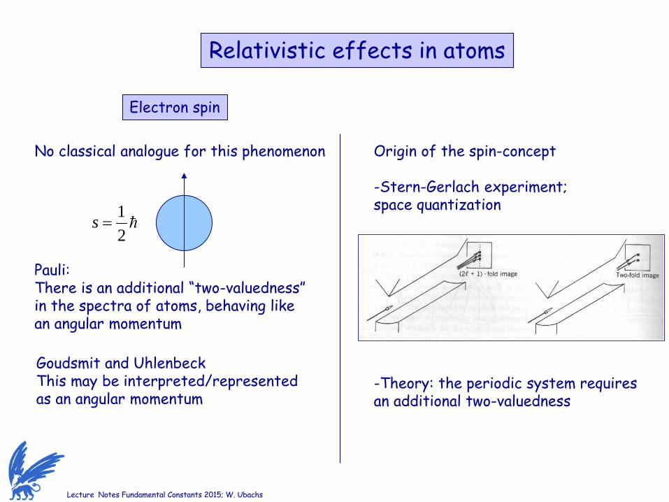
No classical analogue for this phenomenon
Pauli: There is an additional “two-valuedness” in the spectra of atoms, behaving like an angular momentum
21
=s
Goudsmit and Uhlenbeck This may be interpreted/represented as an angular momentum
Origin of the spin-concept -Stern-Gerlach experiment; space quantization -Theory: the periodic system requires an additional two-valuedness
Electron spin
Lecture Notes Fundamental Constants 2015; W. Ubachs
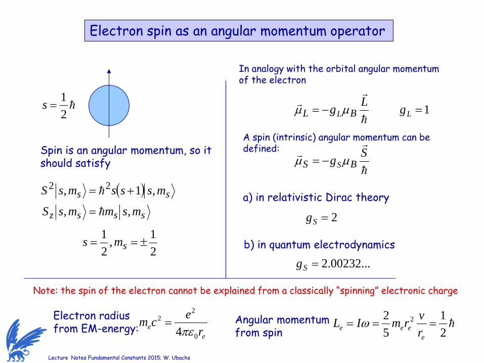
Electron spin as an angular momentum operator
21
=s
Spin is an angular momentum, so it should satisfy
( ) ss msssmsS ,1, 22 +=
sssz msmmsS ,, =
21,
21
±== sms
Lg BL Lµµ −=
In analogy with the orbital angular momentum of the electron
A spin (intrinsic) angular momentum can be defined:
Sg BS S µµ −=
2=Sg
1=Lg
a) in relativistic Dirac theory
b) in quantum electrodynamics
...00232.2=Sg
Note: the spin of the electron cannot be explained from a classically “spinning” electronic charge
Electron radius from EM-energy:
ee r
ecm0
22
4πε= Angular momentum
from spin
21
52 2 ===
eeee r
vrmIL ω
Lecture Notes Fundamental Constants 2015; W. Ubachs
Spin-orbit interaction
Frame of nucleus:
+Ze
-e
v
+Ze
-e
v−
Frame of electron:
The moving charged nucleus induces a magnetic field at the location of the electron, via Biot-Savart’s law
( )3
04 r
rvZeB ×−
=π
µ
Use vrmL ×= 200
1c
=εµ;
Then 320int 4 rcm
LZeBe
πε=
Spin of electron is a magnet with dipole
Sg BeS
µµ −=
The dipole orients in the B-field with energy
LSrcm
ZeBVe
SLS
⋅=⋅−= 3220
2
4πεµ
A fully relativistic derivation (Thomas Precession) yields with
( ) LSrVLS
⋅= ζ
( )nle rcm
Zer 3220
2 18πε
ζ =
Use:
( )( )
( )( )12/12
12/121
3
3
333
++
=++
=
nnmcZ
nar
α
Lecture Notes Fundamental Constants 2015; W. Ubachs
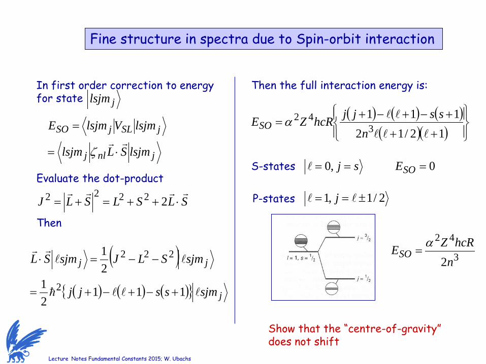
Fine structure in spectra due to Spin-orbit interaction
jnlj
jSLjSO
lsjmSLlsjm
lsjmVlsjmE
⋅=
=
ζ
In first order correction to energy for state
Evaluate the dot-product
SLSLSLJ
⋅++=+= 22222
Then
( )( ) ( ) ( ){ } j
jj
sjmssjj
sjmSLJsjmSL
11121
21
2
222
+−+−+=
−−=⋅
Then the full interaction energy is:
( ) ( ) ( )( )( )
++
+−+−+=
12/12111
342
nssjjhcRZESO α
S-states 0=SOEsj == ,0
P-states
3
42
2nhcRZESO
α=
2/1,1 ±== j
jlsjm
Show that the “centre-of-gravity” does not shift
Lecture Notes Fundamental Constants 2015; W. Ubachs
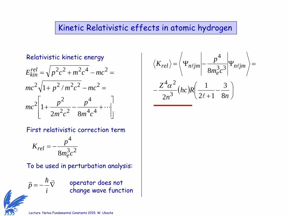
Kinetic Relativistic effects in atomic hydrogen
Relativistic kinetic energy
+−+
=−+
=−+=
44
4
22
22
22222
24222
821
/1
cmp
cmpmc
mccmpmc
mccmcpErelkin
First relativistic correction term
23
4
8 cmpKe
rel −=
To be used in perturbation analysis:
( )
−
+−
=Ψ−Ψ=
nRhc
nZ
cmpK jmne
jmnrel
83
121
2
8
3
24
33
4
α
∇−=
ip operator does not
change wave function
Lecture Notes Fundamental Constants 2015; W. Ubachs
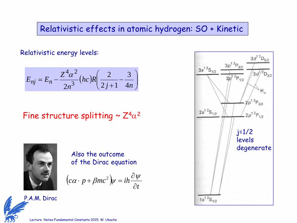
Relativistic effects in atomic hydrogen: SO + Kinetic
Relativistic energy levels:
( )
−
+−=
njRhc
nZEE nnj 4
312
22 3
24α
j=1/2 levels degenerate
P.A.M. Dirac
Also the outcome of the Dirac equation
( )t
ihmcpc∂
∂=+⋅
ψψβα 2
Fine structure splitting ~ Z4α2
Lecture Notes Fundamental Constants 2015; W. Ubachs
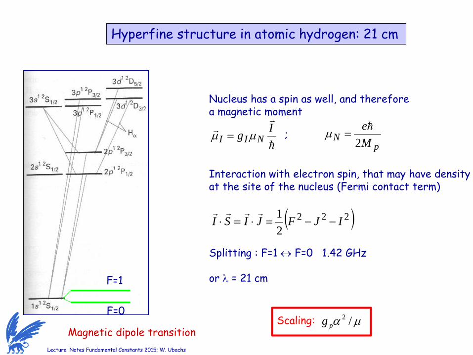
Hyperfine structure in atomic hydrogen: 21 cm
F=1
F=0
Nucleus has a spin as well, and therefore a magnetic moment
Ig NII µµ = ;
pN M
e2
=µ
Interaction with electron spin, that may have density at the site of the nucleus (Fermi contact term)
( )22221 IJFJISI −−=⋅=⋅
Splitting : F=1 ↔ F=0 1.42 GHz or λ = 21 cm
Magnetic dipole transition Scaling: µα /2
pg
Lecture Notes Fundamental Constants 2015; W. Ubachs
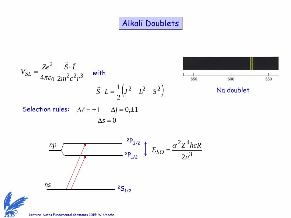
Alkali Doublets
3220
2
24 rcmLSZeVSL
⋅
=πε with
( )22221 SLJLS −−=⋅
Selection rules: 1±=∆ 1,0 ±=∆j0=∆s
ns
np 2P3/2
2P1/2
2S1/2
3
42
2nhcRZESO
α=
Na doublet
Lecture Notes Fundamental Constants 2015; W. Ubachs
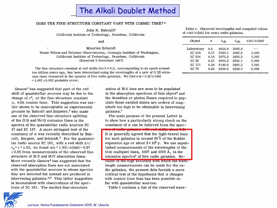
The Alkali Doublet Method
Lecture Notes Fundamental Constants 2015; W. Ubachs
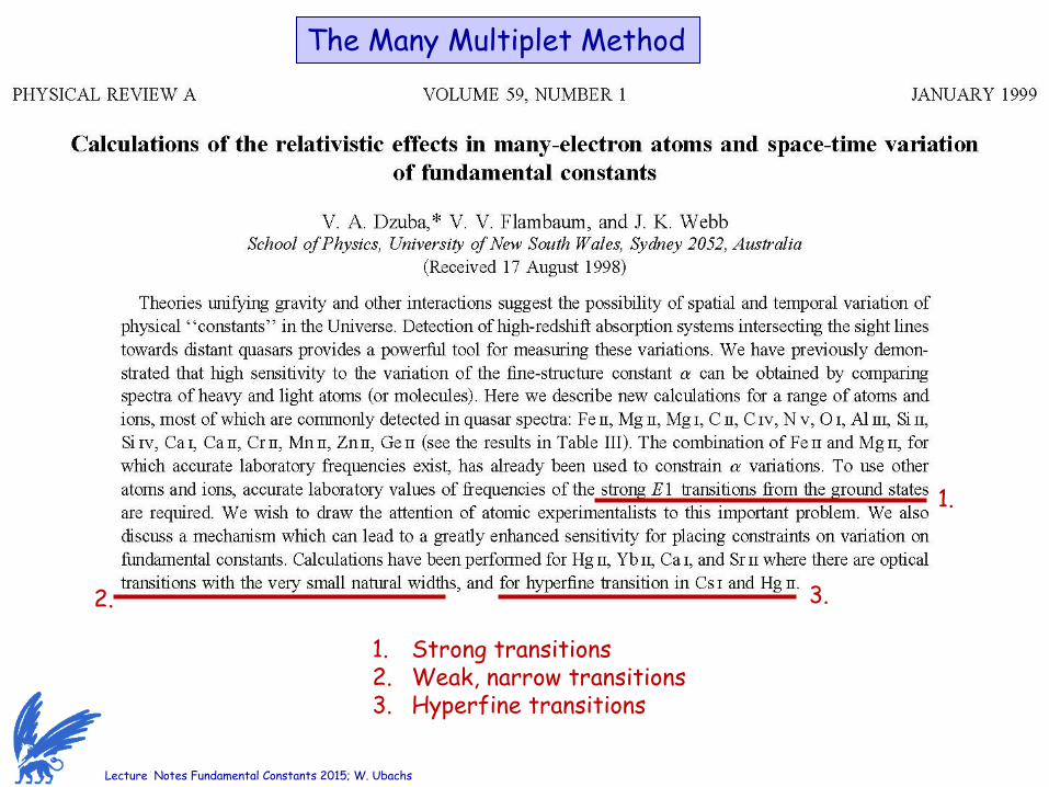
The Many Multiplet Method
1.
2. 3.
1. Strong transitions 2. Weak, narrow transitions 3. Hyperfine transitions
Lecture Notes Fundamental Constants 2015; W. Ubachs
The Many Multiplet Method
∞−= RnZEn 2
2
2
2
0
2
24
emeR
=∞ πε
Lecture Notes Fundamental Constants 2015; W. Ubachs
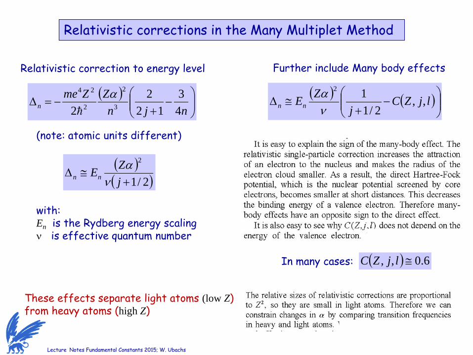
Relativistic corrections in the Many Multiplet Method
( )
−
+−=∆
njnZZme
n 43
122
2 3
2
2
24 α
Relativistic correction to energy level
(note: atomic units different)
( )( )2/1
2
+≅∆
jZEnn ν
α
with: En is the Rydberg energy scaling ν is effective quantum number
Further include Many body effects
( ) ( )
−
+≅∆ ljZC
jZEnn ,,
2/112
να
These effects separate light atoms (low Z) from heavy atoms (high Z)
( ) 6.0,, ≅ljZCIn many cases:
Lecture Notes Fundamental Constants 2015; W. Ubachs
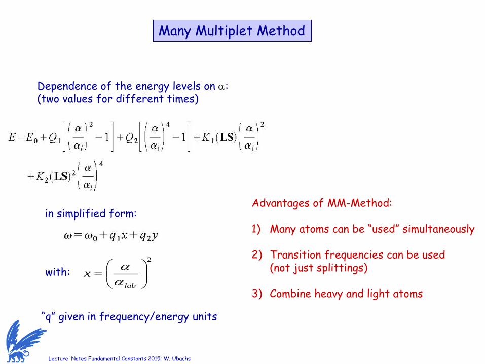
Many Multiplet Method
Dependence of the energy levels on α: (two values for different times)
in simplified form:
with:
Advantages of MM-Method: 1) Many atoms can be “used” simultaneously
2) Transition frequencies can be used (not just splittings) 3) Combine heavy and light atoms
“q” given in frequency/energy units
2
=
lab
xαα
Lecture Notes Fundamental Constants 2015; W. Ubachs
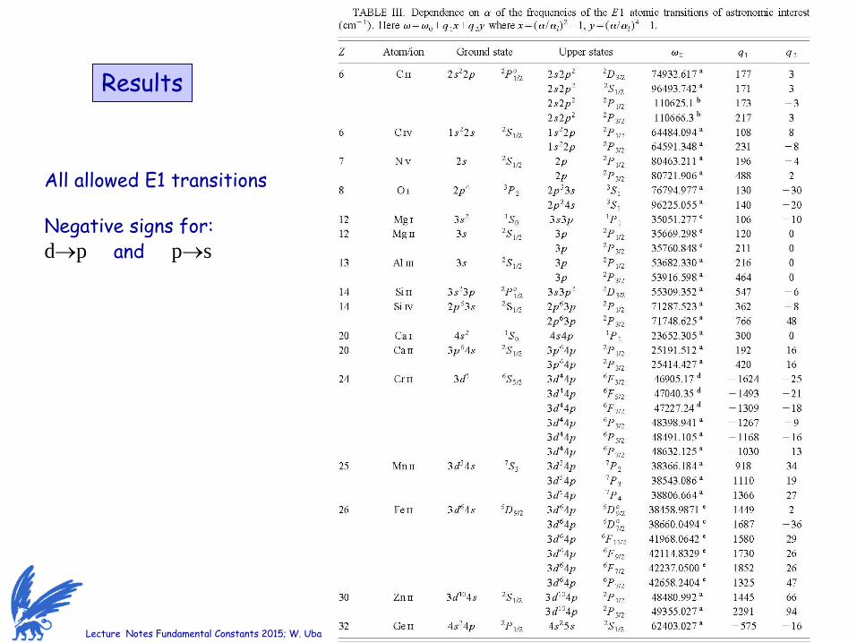
Results
All allowed E1 transitions Negative signs for: d→p and p→s
Lecture Notes Fundamental Constants 2015; W. Ubachs
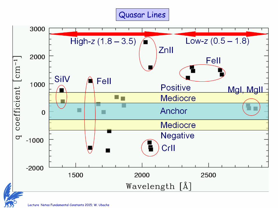
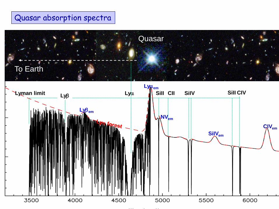
Quasar Lines
Lecture Notes Fundamental Constants 2015; W. Ubachs
( )
+−= 2/30 1
11z
TT
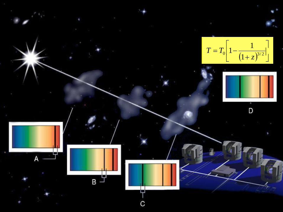
Lecture Notes Fundamental Constants 2015; W. Ubachs
“Quasar Absorptie Spectra”
To Earth
Quasar
CIV SiIV CII SiII Lyαem
Lyman limit Lyα
NVem
SiIVem
Lyβem
Lyβ SiII
CIVem
Quasar absorption spectra
Lecture Notes Fundamental Constants 2015; W. Ubachs
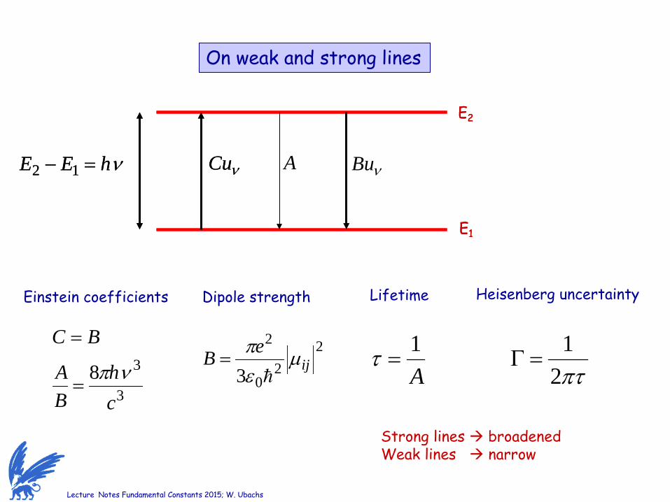
On weak and strong lines
E2
E1
νhEE =− 12 νCu
E2
E1
νhEE =− 12 νCu A νBu
BC =
3
38ch
BA νπ
= A1
=τ
Einstein coefficients
22
0
2
3 ijeB µ
επ
=
Dipole strength Lifetime Heisenberg uncertainty
πτ21
=Γ
Strong lines broadened Weak lines narrow
Lecture Notes Fundamental Constants 2015; W. Ubachs
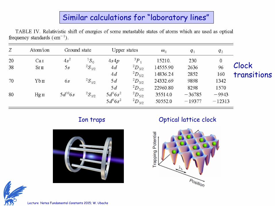
Similar calculations for “laboratory lines”
Clock transitions
Ion traps Optical lattice clock
Lecture Notes Fundamental Constants 2015; W. Ubachs
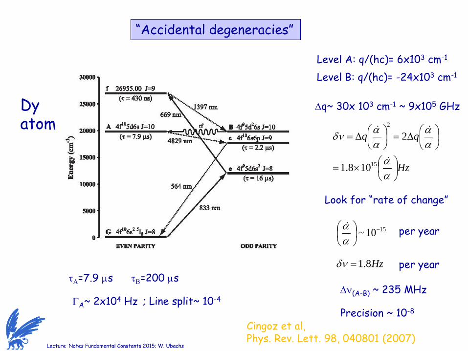
“Accidental degeneracies”
Dy atom
Cingoz et al, Phys. Rev. Lett. 98, 040801 (2007)
Level A: q/(hc)= 6x103 cm-1
Level B: q/(hc)= -24x103 cm-1
∆ν(A-B) ~ 235 MHz
∆q~ 30x 103 cm-1 ~ 9x10⁵ GHz
Hz
×=
∆=
∆=
αα
αα
ααδν
15
2
108.1
2
Look for “rate of change”
1510~ −
αα per year
Hz8.1=δν per year
Precision ~ 10-8
τΒ=200 µs τΑ=7.9 µs
ΓA~ 2x10⁴ Hz ; Line split~ 10-4
Lecture Notes Fundamental Constants 2015; W. Ubachs
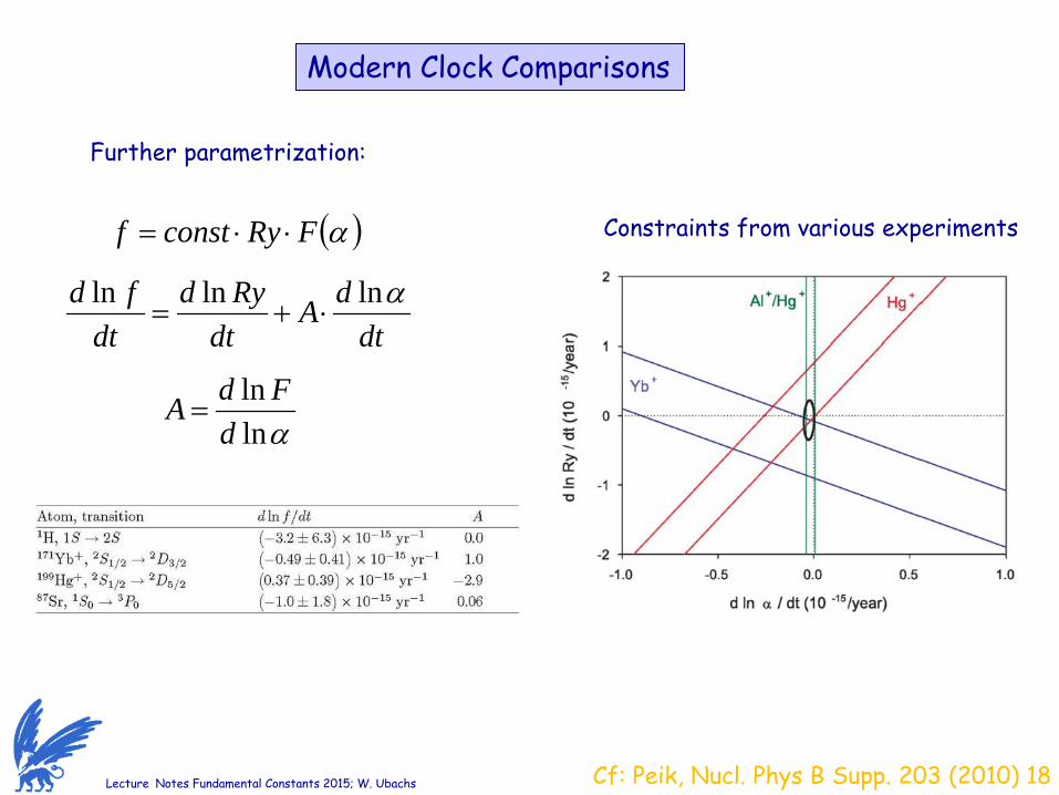
Modern Clock Comparisons
Further parametrization:
( )αFRyconstf ⋅⋅=
dtdA
dtRyd
dtfd αlnlnln
⋅+=
αlnln
dFdA =
Constraints from various experiments
Cf: Peik, Nucl. Phys B Supp. 203 (2010) 18
Lecture Notes Fundamental Constants 2015; W. Ubachs
Functional dependence on fundamental constants