At Aththena Visual Studio A Mo l Tutorial Equations Tutorial.pdf · AtAth. hen. a Visual Studio...
17
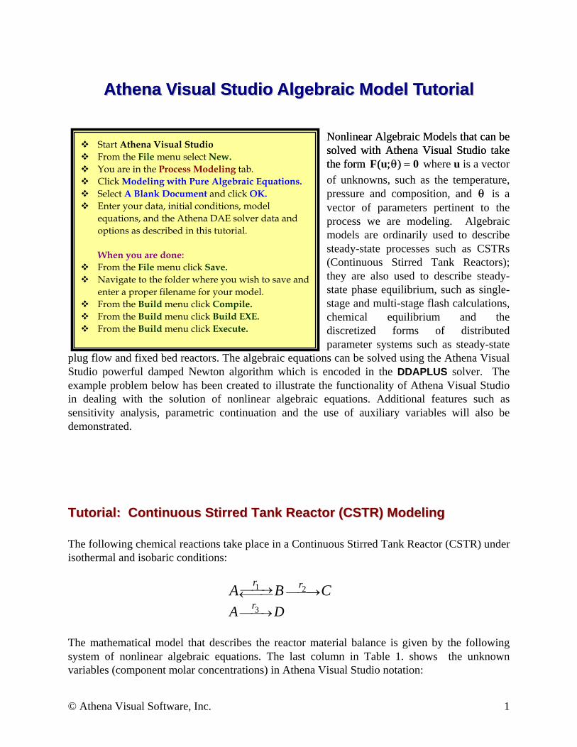
A t hena Visual Studio Algebraic Model Tutorial A Nonlinear Algebraic Models that can be solved with Athena Visual Studio take the form Nonlinear Algebraic Models that can be solved with Athena Visual Studio take the form (;) (;) thena Visual Studio Algebraic Model Tutorial θ = Fu 0 where u is a vector of unknowns, such as the temperature, pressure and composition, and θ is a vector of parameters pertinent to the process we are modeling. Algebraic models are ordinarily used to describe steady-state processes such as CSTRs (Continuous Stirred Tank Reactors); they are also used to describe steady- state phase equilibrium, such as single- stage and multi-stage flash calculations, chemical equilibrium and the discretized forms of distributed parameter systems such as steady-state plug flow and fixed bed reactors. The algebraic equations can be solved using the Athena Visual Studio powerful damped Newton algorithm which is encoded in the DDAPLUS solver. The example problem below has been created to illustrate the functionality of Athena Visual Studio in dealing with the solution of nonlinear algebraic equations. Additional features such as sensitivity analysis, parametric continuation and the use of auxiliary variables will also be demonstrated. Start Athena Visual Studio From the File menu select New. You are in the Process Modeling tab. Click Modeling with Pure Algebraic Equations. Select A Blank Document and click OK. Enter your data, initial conditions, model equations, and the Athena DAE solver data and options as described in this tutorial. When you are done: From the File menu click Save. Navigate to the folder where you wish to save and enter a proper filename for your model. From the Build menu click Compile. From the Build menu click Build EXE. From the Build menu click Execute. Tutorial: Continuous Stirred Tank Reactor (CSTR) Modeling The following chemical reactions take place in a Continuous Stirred Tank Reactor (CSTR) under isothermal and isobaric conditions: 1 2 3 r r r A D A B C ⎯⎯→ ⎯⎯⎯→ ←⎯⎯ ⎯⎯→ The mathematical model that describes the reactor material balance is given by the following system of nonlinear algebraic equations. The last column in Table 1. shows the unknown variables (component molar concentrations) in Athena Visual Studio notation: © Athena Visual Software, Inc. 1
Transcript of At Aththena Visual Studio A Mo l Tutorial Equations Tutorial.pdf · AtAth. hen. a Visual Studio...
AAtthheennaa VViissuuaall SSttuuddiioo AAllggeebbrraaiicc MMooddeell TTuuttoorriiaall AA
Nonlinear Algebraic Models that can be solved with Athena Visual Studio take the form
Nonlinear Algebraic Models that can be solved with Athena Visual Studio take the form ( ; )( ; )
tthheennaa VViissuuaall SSttuuddiioo AAllggeebbrraaiicc MMooddeell TTuuttoorriiaall
θ =F u 0 where u is a vector of unknowns, such as the temperature, pressure and composition, and θ is a vector of parameters pertinent to the process we are modeling. Algebraic models are ordinarily used to describe steady-state processes such as CSTRs (Continuous Stirred Tank Reactors); they are also used to describe steady-state phase equilibrium, such as single-stage and multi-stage flash calculations, chemical equilibrium and the discretized forms of distributed parameter systems such as steady-state
plug flow and fixed bed reactors. The algebraic equations can be solved using the Athena Visual Studio powerful damped Newton algorithm which is encoded in the DDAPLUS solver. The example problem below has been created to illustrate the functionality of Athena Visual Studio in dealing with the solution of nonlinear algebraic equations. Additional features such as sensitivity analysis, parametric continuation and the use of auxiliary variables will also be demonstrated.
Start Athena Visual Studio From the File menu select New. You are in the Process Modeling tab. Click Modeling with Pure Algebraic Equations. Select A Blank Document and click OK. Enter your data, initial conditions, model
equations, and the Athena DAE solver data and options as described in this tutorial.
When you are done: From the File menu click Save. Navigate to the folder where you wish to save and
enter a proper filename for your model. From the Build menu click Compile. From the Build menu click Build EXE. From the Build menu click Execute.
TTuuttoorriiaall:: CCoonnttiinnuuoouuss SSttiirrrreedd TTaannkk RReeaaccttoorr ((CCSSTTRR)) MMooddeelliinngg The following chemical reactions take place in a Continuous Stirred Tank Reactor (CSTR) under isothermal and isobaric conditions:
1 2
3
r r
rA DA B C⎯⎯→ ⎯⎯⎯→←⎯⎯
⎯⎯→
The mathematical model that describes the reactor material balance is given by the following system of nonlinear algebraic equations. The last column in Table 1. shows the unknown variables (component molar concentrations) in Athena Visual Studio notation:
© Athena Visual Software, Inc. 1
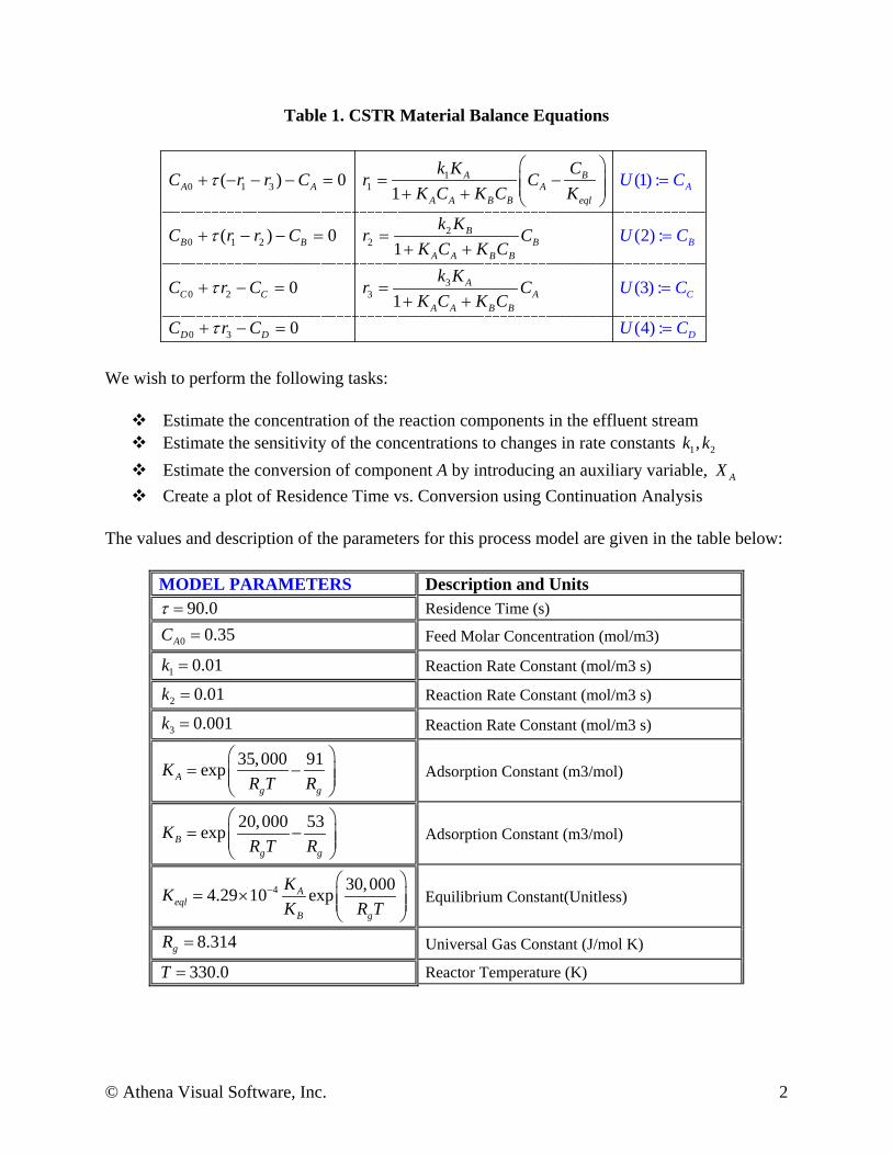
Table 1. CSTR Material Balance Equations
10 1 3 1
20 1 2 2
30 2 3
0 3
(1) :
(2) :
(3) :
( ) 01
( ) 01
0
(4 :1
0 )
AA B
A A AA A B B eql
BB B B
A A B B
AC C A
A A B B
D
C
D
B
D
k K CC r r C r C
K C K C K
k KC r r C r C
K C K Ck K
C r C r CK C
U C
U C
U C
U CK C
C r C
τ
τ
τ
τ
⎛ ⎞+ − − − = = −⎜ ⎟⎜ ⎟+ + ⎝ ⎠
+ − − = =
=
=
=
+ +
+ − = =+ +
+ − ==
We wish to perform the following tasks:
Estimate the concentration of the reaction components in the effluent stream Estimate the sensitivity of the concentrations to changes in rate constants 1 2 ,k k Estimate the conversion of component A by introducing an auxiliary variable, AX Create a plot of Residence Time vs. Conversion using Continuation Analysis
The values and description of the parameters for this process model are given in the table below:
MODEL PARAMETERS Description and Units 90.0τ = Residence Time (s)
0 0.35AC = Feed Molar Concentration (mol/m3)
1 0.01k = Reaction Rate Constant (mol/m3 s)
2 0.01k = Reaction Rate Constant (mol/m3 s)
3 0.001k = Reaction Rate Constant (mol/m3 s)
35,000 91expAg g
KR T R
⎛ ⎞= −⎜ ⎟⎜ ⎟
⎝ ⎠ Adsorption Constant (m3/mol)
20,000 53expBg g
KR T R
⎛ ⎞= −⎜⎜
⎝ ⎠⎟⎟ Adsorption Constant (m3/mol)
4 30,0004.29 10 expAeql
B g
KKK R T
−⎛ ⎞
= × ⎜⎜⎝ ⎠
⎟⎟ Equilibrium Constant(Unitless)
8.314gR = Universal Gas Constant (J/mol K)
330.0T = Reactor Temperature (K)
© Athena Visual Software, Inc. 2
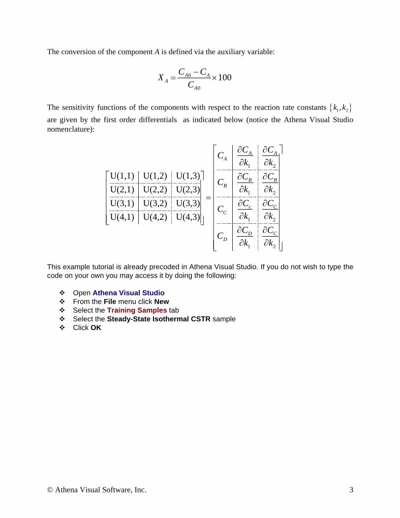
The conversion of the component A is defined via the auxiliary variable:
0
0
100A AA
A
C CXC−
= ×
The sensitivity functions of the components with respect to the reaction rate constants { }1 2,k k are given by the first order differentials as indicated below (notice the Athena Visual Studio nomenclature):
1 2
1 2
1 2
1 2
U(1,1) U(1,2) U(1,3)U(2,1) U(2,2) U(2,3)U(3,1) U(3,2) U(3,3)U(4,1) U(4,2) U(4,3)
A AA
B BB
c CC
D CD
C CCk kC CCk kC CCk kC CCk k
∂ ∂⎡ ⎤⎢ ⎥∂ ∂⎢ ⎥
∂ ∂⎡ ⎤ ⎢ ⎥⎢ ⎥ ⎢ ⎥∂ ∂⎢ ⎥ ⎢ ⎥=⎢ ⎥ ∂ ∂⎢ ⎥⎢ ⎥ ⎢ ⎥∂ ∂⎢ ⎥ ⎢ ⎥⎣ ⎦
⎢ ⎥∂ ∂⎢ ⎥∂ ∂⎢ ⎥⎣ ⎦
This example tutorial is already precoded in Athena Visual Studio. If you do not wish to type the code on your own you may access it by doing the following:
Open Athena Visual Studio From the File menu click New Select the Training Samples tab Select the Steady-State Isothermal CSTR sample Click OK
© Athena Visual Software, Inc. 3
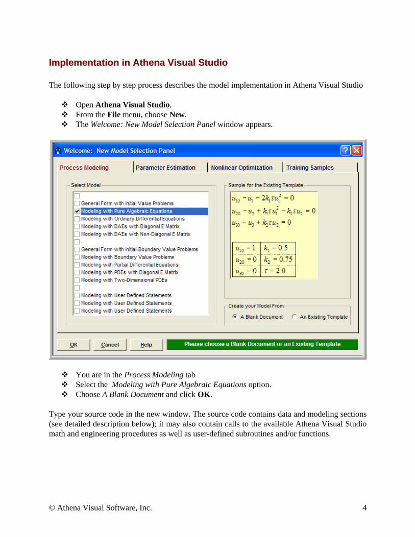
IImmpplleemmeennttaattiioonn iinn AAtthheennaa VViissuuaall SSttuuddiioo The following step by step process describes the model implementation in Athena Visual Studio
Open Athena Visual Studio. From the File menu, choose New. The Welcome: New Model Selection Panel window appears.
You are in the Process Modeling tab Select the Modeling with Pure Algebraic Equations option. Choose A Blank Document and click OK.
Type your source code in the new window. The source code contains data and modeling sections (see detailed description below); it may also contain calls to the available Athena Visual Studio math and engineering procedures as well as user-defined subroutines and/or functions.
© Athena Visual Software, Inc. 4

WWrriittiinngg tthhee SSoouurrccee CCooddee The user must enter a minimum of two sections in order to create the algebraic model. The first section labeled @Initial Conditions is used to insert initial guesses for the unknown vector. These initial guesses are used by the Newton method to start the iterative algorithm. The second section labeled @Model Equations is used to enter the model equations. A data section not labeled by Athena Visual Studio is used to enter all the data pertinent to the model. The data section also contains the declaration statements for all model variables, parameters and constants. This section, if used, must be the first one. The declaration of the model variables, parameters and constants must be done in accordance the Athena Visual Studio syntax rules detailed below:
DDaattaa SSeeccttiioonn In the data section the user simply enters the problem data and various constants. In this example the user enters values for residence time, reactor temperature, initial feed concentration and miscellaneous other reaction parameters. The Athena interpreter treats any line that begins with the exclamation mark ! as a comment. It is mandatory and strongly recommended that the users declare all the problem variables, parameters and constants. All variables in Athena are either real double or single precision or integer long. Character and Logical variables are also allowed. The following source code may be entered for this example (If you use the Windows Copy and Paste commands to enter this code into your Athena Visual Studio project, please beware that invisible format symbols may also be copied and cause the compilation of your code to fail): ! Declarations and Model Constants !================================= Global k1,k2,k3,Keql,Ka,Kb As Real Global Temp,Rg,Tau As Real Global CAo,CBo,CCo,CDo As Real Global CA,CB,CC,CD As Real Rg=8.314 ! Universal Gas Constant (J/mole K) Tau=90.0 ! Residence Time (s) Temp=330.0 ! Temperature (K) CAo=0.35 ! Initial Concentration of A (mol/m3) CBo=0.0 ! Initial Concentration of B (mol/m3) CCo=0.0 ! Initial Concentration of C (mol/m3) CDo=0.0 ! Initial Concentration of D (mol/m3) k1=0.01 ! Reaction rate coefficient (mol/m3 s) k2=0.01 ! Reaction rate coefficient (mol/m3 s) k3=0.001 ! Reaction rate coefficient (mol/m3 s) Ka=exp(35000.0/Rg/Temp-91.0/Rg) ! Adsorption constant (m3/mol) Kb=exp(20000.0/Rg/Temp-53.0/Rg) ! Adsorption constant (m3/mol) Keql=4.29E-4*Ka/Kb*exp(30000.0/Rg/Temp) ! Equilibrium constant
© Athena Visual Software, Inc. 5
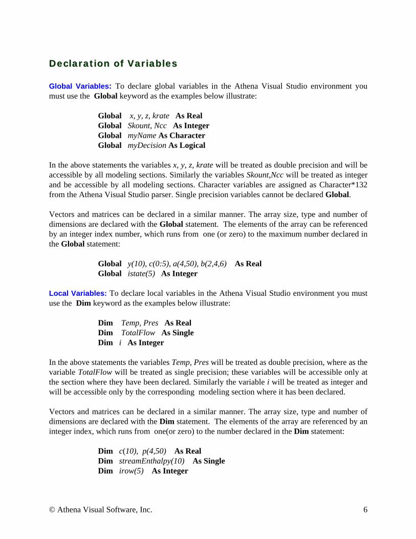
DDeeccllaarraattiioonn ooff VVaarriiaabblleess Global Variables: To declare global variables in the Athena Visual Studio environment you must use the Global keyword as the examples below illustrate:
Global x, y, z, krate As Real Global Skount, Ncc As Integer Global myName As Character Global myDecision As Logical
In the above statements the variables x, y, z, krate will be treated as double precision and will be accessible by all modeling sections. Similarly the variables Skount,Ncc will be treated as integer and be accessible by all modeling sections. Character variables are assigned as Character*132 from the Athena Visual Studio parser. Single precision variables cannot be declared Global. Vectors and matrices can be declared in a similar manner. The array size, type and number of dimensions are declared with the Global statement. The elements of the array can be referenced by an integer index number, which runs from one (or zero) to the maximum number declared in the Global statement:
Global y(10), c(0:5), a(4,50), b(2,4,6) As Real Global istate(5) As Integer
Local Variables: To declare local variables in the Athena Visual Studio environment you must use the Dim keyword as the examples below illustrate:
Dim Temp, Pres As Real Dim TotalFlow As Single Dim i As Integer
In the above statements the variables Temp, Pres will be treated as double precision, where as the variable TotalFlow will be treated as single precision; these variables will be accessible only at the section where they have been declared. Similarly the variable i will be treated as integer and will be accessible only by the corresponding modeling section where it has been declared. Vectors and matrices can be declared in a similar manner. The array size, type and number of dimensions are declared with the Dim statement. The elements of the array are referenced by an integer index, which runs from one(or zero) to the number declared in the Dim statement:
Dim c(10), p(4,50) As Real Dim streamEnthalpy(10) As Single Dim irow(5) As Integer
© Athena Visual Software, Inc. 6
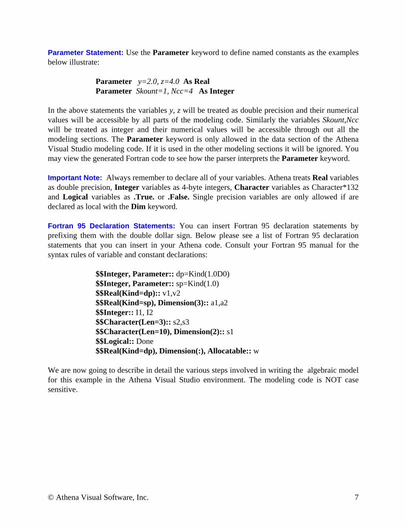
Parameter Statement: Use the Parameter keyword to define named constants as the examples below illustrate:
Parameter y=2.0, z=4.0 As Real Parameter Skount=1, Ncc=4 As Integer
In the above statements the variables y, z will be treated as double precision and their numerical values will be accessible by all parts of the modeling code. Similarly the variables Skount,Ncc will be treated as integer and their numerical values will be accessible through out all the modeling sections. The Parameter keyword is only allowed in the data section of the Athena Visual Studio modeling code. If it is used in the other modeling sections it will be ignored. You may view the generated Fortran code to see how the parser interprets the Parameter keyword. Important Note: Always remember to declare all of your variables. Athena treats Real variables as double precision, Integer variables as 4-byte integers, Character variables as Character*132 and Logical variables as .True. or .False. Single precision variables are only allowed if are declared as local with the Dim keyword. Fortran 95 Declaration Statements: You can insert Fortran 95 declaration statements by prefixing them with the double dollar sign. Below please see a list of Fortran 95 declaration statements that you can insert in your Athena code. Consult your Fortran 95 manual for the syntax rules of variable and constant declarations:
$$Integer, Parameter:: dp=Kind(1.0D0) $$Integer, Parameter:: sp=Kind(1.0) $$Real(Kind=dp):: v1,v2 $$Real(Kind=sp), Dimension(3):: a1,a2 $$Integer:: I1, I2 $$Character(Len=3):: s2,s3 $$Character(Len=10), Dimension(2):: s1 $$Logical:: Done $$Real(Kind=dp), Dimension(:), Allocatable:: w
We are now going to describe in detail the various steps involved in writing the algebraic model for this example in the Athena Visual Studio environment. The modeling code is NOT case sensitive.
© Athena Visual Software, Inc. 7
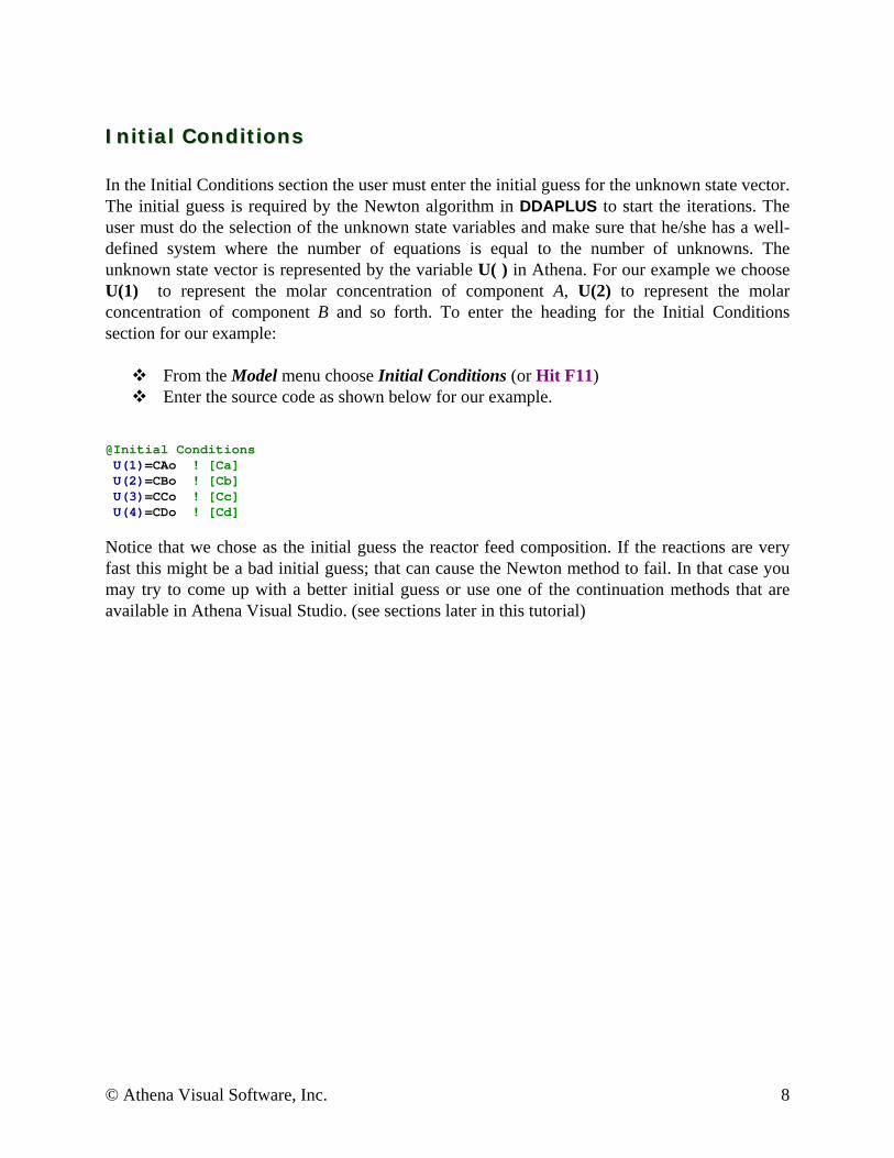
IInniittiiaall CCoonnddiittiioonnss In the Initial Conditions section the user must enter the initial guess for the unknown state vector. The initial guess is required by the Newton algorithm in DDAPLUS to start the iterations. The user must do the selection of the unknown state variables and make sure that he/she has a well-defined system where the number of equations is equal to the number of unknowns. The unknown state vector is represented by the variable U( ) in Athena. For our example we choose U(1) to represent the molar concentration of component A, U(2) to represent the molar concentration of component B and so forth. To enter the heading for the Initial Conditions section for our example:
From the Model menu choose Initial Conditions (or Hit F11) Enter the source code as shown below for our example.
@Initial Conditions U(1)=CAo ! [Ca] U(2)=CBo ! [Cb] U(3)=CCo ! [Cc] U(4)=CDo ! [Cd]
Notice that we chose as the initial guess the reactor feed composition. If the reactions are very fast this might be a bad initial guess; that can cause the Newton method to fail. In that case you may try to come up with a better initial guess or use one of the continuation methods that are available in Athena Visual Studio. (see sections later in this tutorial)
© Athena Visual Software, Inc. 8
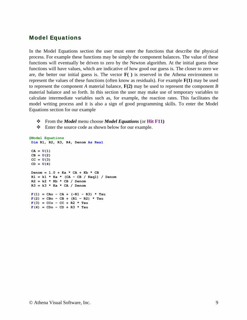
MMooddeell EEqquuaattiioonnss In the Model Equations section the user must enter the functions that describe the physical process. For example these functions may be simply the component balances. The value of these functions will eventually be driven to zero by the Newton algorithm. At the initial guess these functions will have values, which are indicative of how good our guess is. The closer to zero we are, the better our initial guess is. The vector F( ) is reserved in the Athena environment to represent the values of these functions (often know as residuals). For example F(1) may be used to represent the component A material balance, F(2) may be used to represent the component B material balance and so forth. In this section the user may make use of temporary variables to calculate intermediate variables such as, for example, the reaction rates. This facilitates the model writing process and it is also a sign of good programming skills. To enter the Model Equations section for our example
From the Model menu choose Model Equations (or Hit F11) Enter the source code as shown below for our example.
@Model Equations Dim R1, R2, R3, R4, Denom As Real CA = U(1) CB = U(2) CC = U(3) CD = U(4) Denom = 1.0 + Ka * CA + Kb * CB R1 = k1 * Ka * (CA - CB / Keql) / Denom R2 = k2 * Kb * CB / Denom R3 = k3 * Ka * CA / Denom F(1) = CAo - CA + (-R1 - R3) * Tau F(2) = CBo - CB + (R1 - R2) * Tau F(3) = CCo - CC + R2 * Tau F(4) = CDo - CD + R3 * Tau
© Athena Visual Software, Inc. 9
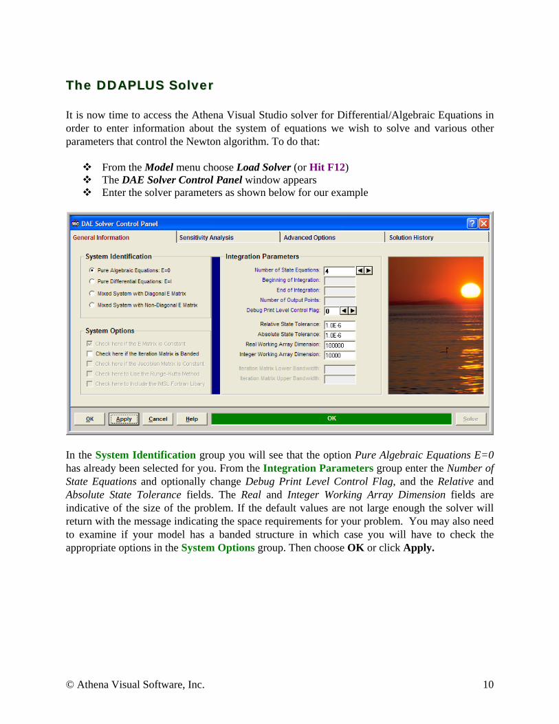
TThhee DDDDAAPPLLUUSS SSoollvveerr It is now time to access the Athena Visual Studio solver for Differential/Algebraic Equations in order to enter information about the system of equations we wish to solve and various other parameters that control the Newton algorithm. To do that:
From the Model menu choose Load Solver (or Hit F12) The DAE Solver Control Panel window appears Enter the solver parameters as shown below for our example
In the System Identification group you will see that the option Pure Algebraic Equations E=0 has already been selected for you. From the Integration Parameters group enter the Number of State Equations and optionally change Debug Print Level Control Flag, and the Relative and Absolute State Tolerance fields. The Real and Integer Working Array Dimension fields are indicative of the size of the problem. If the default values are not large enough the solver will return with the message indicating the space requirements for your problem. You may also need to examine if your model has a banded structure in which case you will have to check the appropriate options in the System Options group. Then choose OK or click Apply.
© Athena Visual Software, Inc. 10
SSaavviinngg aanndd RRuunnnniinngg You are now ready to save your model and run it. New files are labeled UNTITLED until they are saved. Keep in mind that the maximum number of characters in a line is 132; the maximum number of lines in a file is infinity. In order to save your project:
From the File menu, choose Save. The Save As dialog box appears. This action saves your model and creates the Fortran code. In the Directories box, double-click a directory where you want to store the source file. Type a filename (a filename cannot contain the following characters: \ / : * ? “ < > |) in
the File Name box, then choose OK. The default extension is avw To view the Fortran code that you have just created from the View menu choose Fortran
Code. You may now choose to compile, build and execute your project; to do that:
From the Build menu choose Compile (or Hit F2) From the Build menu choose Build EXE (or Hit F4) From the Build menu choose Execute (or Hit F5)
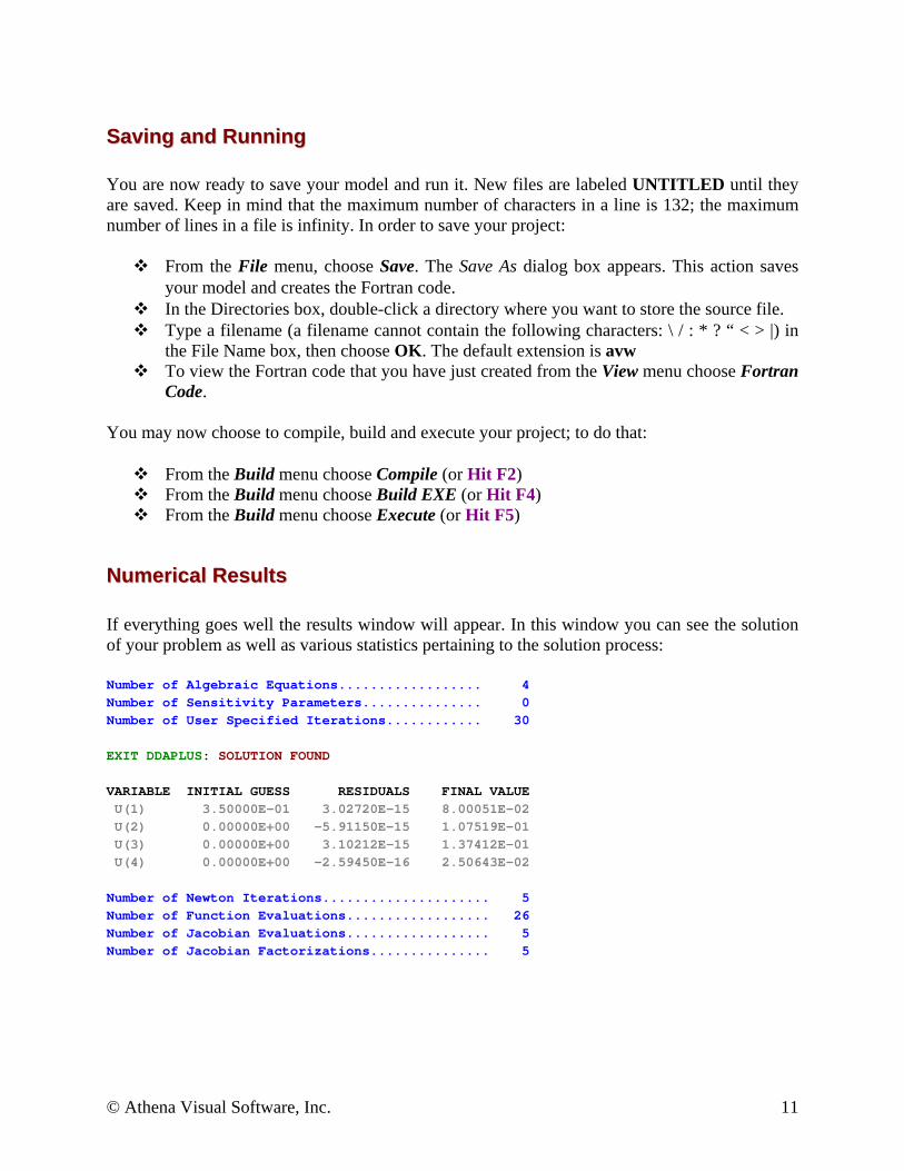
NNuummeerriiccaall RReessuullttss If everything goes well the results window will appear. In this window you can see the solution of your problem as well as various statistics pertaining to the solution process: Number of Algebraic Equations.................. 4 Number of Sensitivity Parameters............... 0 Number of User Specified Iterations............ 30 EXIT DDAPLUS: SOLUTION FOUND VARIABLE INITIAL GUESS RESIDUALS FINAL VALUE U(1) 3.50000E-01 3.02720E-15 8.00051E-02 U(2) 0.00000E+00 -5.91150E-15 1.07519E-01 U(3) 0.00000E+00 3.10212E-15 1.37412E-01 U(4) 0.00000E+00 -2.59450E-16 2.50643E-02 Number of Newton Iterations..................... 5 Number of Function Evaluations.................. 26 Number of Jacobian Evaluations.................. 5 Number of Jacobian Factorizations............... 5
© Athena Visual Software, Inc. 11
SSensitivity Analysis ensitivity Analysis Athena Visual Studio allows for convenient and efficient calculation of the first order sensitivity functions given by:
( ) ∂=∂uW θθ
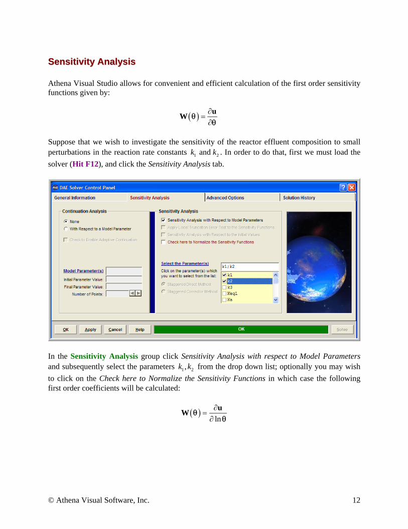
Suppose that we wish to investigate the sensitivity of the reactor effluent composition to small perturbations in the reaction rate constants . In order to do that, first we must load the solver (Hit F12), and click the Sensitivity Analysis tab.
1 and k 2k
In the Sensitivity Analysis group click Sensitivity Analysis with respect to Model Parameters and subsequently select the parameters from the drop down list; optionally you may wish to click on the Check here to Normalize the Sensitivity Functions in which case the following first order coefficients will be calculated:
1 2,k k
( )ln∂
=∂
uW θθ
© Athena Visual Software, Inc. 12
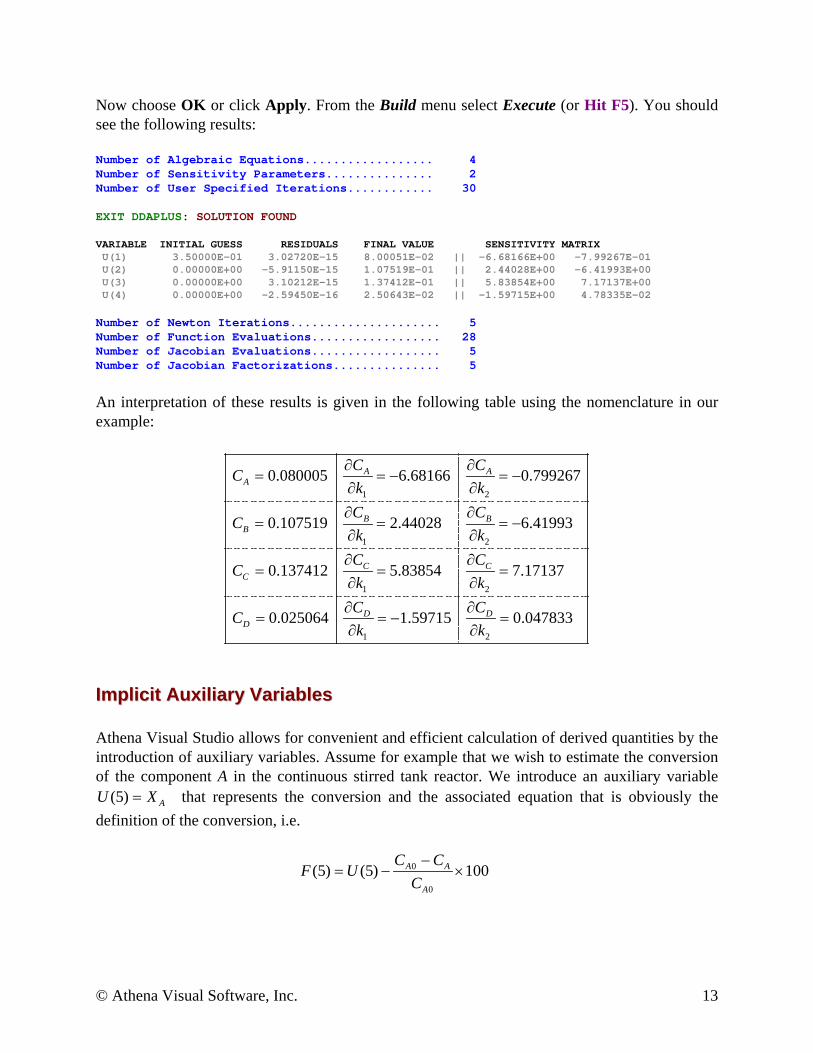
Now choose OK or click Apply. From the Build menu select Execute (or Hit F5). You should see the following results: Number of Algebraic Equations.................. 4 Number of Sensitivity Parameters............... 2 Number of User Specified Iterations............ 30 EXIT DDAPLUS: SOLUTION FOUND VARIABLE INITIAL GUESS RESIDUALS FINAL VALUE SENSITIVITY MATRIX U(1) 3.50000E-01 3.02720E-15 8.00051E-02 || -6.68166E+00 -7.99267E-01 U(2) 0.00000E+00 -5.91150E-15 1.07519E-01 || 2.44028E+00 -6.41993E+00 U(3) 0.00000E+00 3.10212E-15 1.37412E-01 || 5.83854E+00 7.17137E+00 U(4) 0.00000E+00 -2.59450E-16 2.50643E-02 || -1.59715E+00 4.78335E-02 Number of Newton Iterations..................... 5 Number of Function Evaluations.................. 28 Number of Jacobian Evaluations.................. 5 Number of Jacobian Factorizations............... 5
An interpretation of these results is given in the following table using the nomenclature in our example:
1 2
1 2
1 2
1 2
0.080005 6.68166 0.799267
0.107519 2.44028 6.41993
0.137412 5.83854 7.17137
0.025064 1.59715 0.047833
A AA
B BB
C CC
D DD
C CC
k kC C
Ck kC C
Ck kC C
Ck k
∂ ∂= = − = −
∂ ∂∂ ∂
= = = −∂ ∂∂ ∂
= = =∂ ∂∂ ∂
= = − =∂ ∂
IImmpplliicciitt AAuuxxiilliiaarryy VVaarriiaabblleess Athena Visual Studio allows for convenient and efficient calculation of derived quantities by the introduction of auxiliary variables. Assume for example that we wish to estimate the conversion of the component A in the continuous stirred tank reactor. We introduce an auxiliary variable
that represents the conversion and the associated equation that is obviously the definition of the conversion, i.e.
(5) AU X=
0
0
(5) (5) 100A A
A
C CF U
C−
= − ×
© Athena Visual Software, Inc. 13
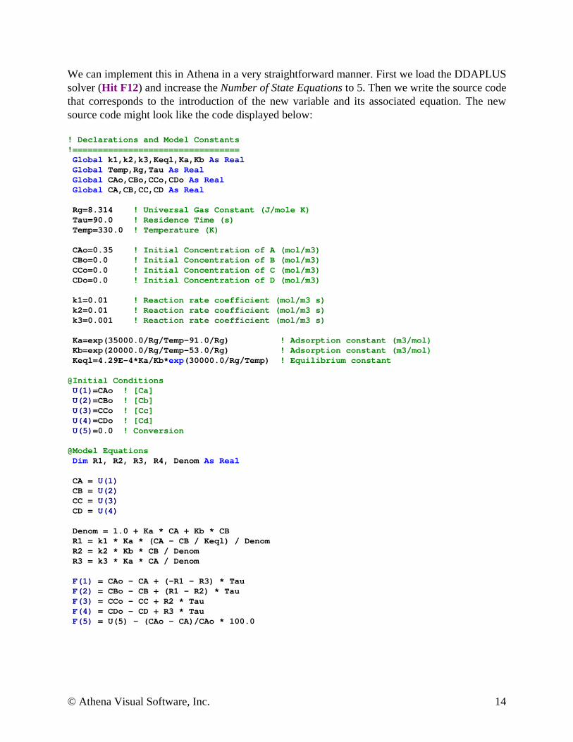
We can implement this in Athena in a very straightforward manner. First we load the DDAPLUS solver (Hit F12) and increase the Number of State Equations to 5. Then we write the source code that corresponds to the introduction of the new variable and its associated equation. The new source code might look like the code displayed below: ! Declarations and Model Constants !================================= Global k1,k2,k3,Keql,Ka,Kb As Real Global Temp,Rg,Tau As Real Global CAo,CBo,CCo,CDo As Real Global CA,CB,CC,CD As Real Rg=8.314 ! Universal Gas Constant (J/mole K) Tau=90.0 ! Residence Time (s) Temp=330.0 ! Temperature (K) CAo=0.35 ! Initial Concentration of A (mol/m3) CBo=0.0 ! Initial Concentration of B (mol/m3) CCo=0.0 ! Initial Concentration of C (mol/m3) CDo=0.0 ! Initial Concentration of D (mol/m3) k1=0.01 ! Reaction rate coefficient (mol/m3 s) k2=0.01 ! Reaction rate coefficient (mol/m3 s) k3=0.001 ! Reaction rate coefficient (mol/m3 s) Ka=exp(35000.0/Rg/Temp-91.0/Rg) ! Adsorption constant (m3/mol) Kb=exp(20000.0/Rg/Temp-53.0/Rg) ! Adsorption constant (m3/mol) Keql=4.29E-4*Ka/Kb*exp(30000.0/Rg/Temp) ! Equilibrium constant @Initial Conditions U(1)=CAo ! [Ca] U(2)=CBo ! [Cb] U(3)=CCo ! [Cc] U(4)=CDo ! [Cd] U(5)=0.0 ! Conversion @Model Equations Dim R1, R2, R3, R4, Denom As Real CA = U(1) CB = U(2) CC = U(3) CD = U(4) Denom = 1.0 + Ka * CA + Kb * CB R1 = k1 * Ka * (CA - CB / Keql) / Denom R2 = k2 * Kb * CB / Denom R3 = k3 * Ka * CA / Denom F(1) = CAo - CA + (-R1 - R3) * Tau F(2) = CBo - CB + (R1 - R2) * Tau F(3) = CCo - CC + R2 * Tau F(4) = CDo - CD + R3 * Tau F(5) = U(5) – (CAo – CA)/CAo * 100.0
© Athena Visual Software, Inc. 14
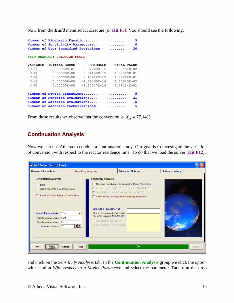
Now from the Build menu select Execute (or Hit F5). You should see the following: Number of Algebraic Equations.................. 5 Number of Sensitivity Parameters............... 0 Number of User Specified Iterations............ 30 EXIT DDAPLUS: SOLUTION FOUND VARIABLE INITIAL GUESS RESIDUALS FINAL VALUE U(1) 3.50000E-01 3.02720E-15 8.00051E-02 U(2) 0.00000E+00 -5.91150E-15 1.07519E-01 U(3) 0.00000E+00 3.10212E-15 1.37412E-01 U(4) 0.00000E+00 -2.59450E-16 2.50643E-02 U(5) 0.00000E+00 -8.27047E-14 7.71414E+01 Number of Newton Iterations..................... 5 Number of Function Evaluations.................. 31 Number of Jacobian Evaluations.................. 5 Number of Jacobian Factorizations............... 5
From these results we observe that the conversion is 77.14%AX =
CCoonnttiinnuuaattiioonn AAnnaallyyssiiss Now we can use Athena to conduct a continuation study. Our goal is to investigate the variation of conversion with respect to the reactor residence time. To do that we load the solver (Hit F12),
and click on the Sensitivity Analysis tab. In the Continuation Analysis group we click the option with caption With respect to a Model Parameter and select the parameter Tau from the drop
© Athena Visual Software, Inc. 15
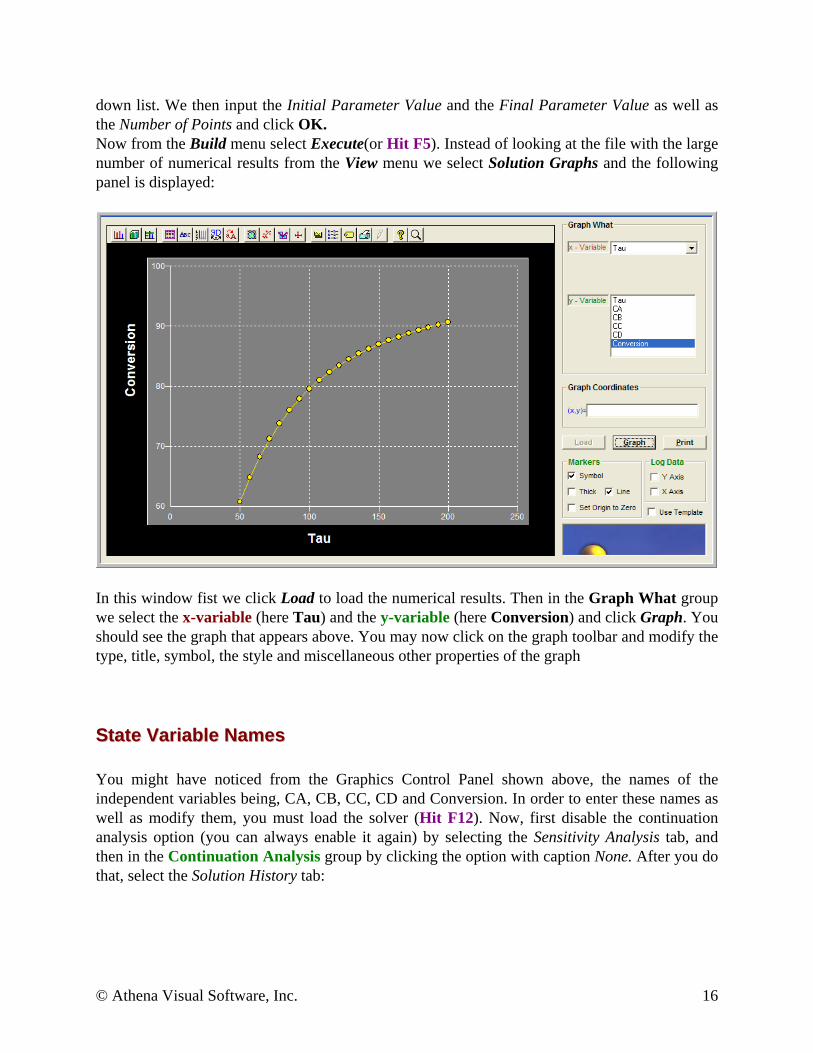
down list. We then input the Initial Parameter Value and the Final Parameter Value as well as the Number of Points and click OK. Now from the Build menu select Execute(or Hit F5). Instead of looking at the file with the large number of numerical results from the View menu we select Solution Graphs and the following panel is displayed:
In this window fist we click Load to load the numerical results. Then in the Graph What group we select the x-variable (here Tau) and the y-variable (here Conversion) and click Graph. You should see the graph that appears above. You may now click on the graph toolbar and modify the type, title, symbol, the style and miscellaneous other properties of the graph
SSttaattee VVaarriiaabbllee NNaammeess You might have noticed from the Graphics Control Panel shown above, the names of the independent variables being, CA, CB, CC, CD and Conversion. In order to enter these names as well as modify them, you must load the solver (Hit F12). Now, first disable the continuation analysis option (you can always enable it again) by selecting the Sensitivity Analysis tab, and then in the Continuation Analysis group by clicking the option with caption None. After you do that, select the Solution History tab:
© Athena Visual Software, Inc. 16
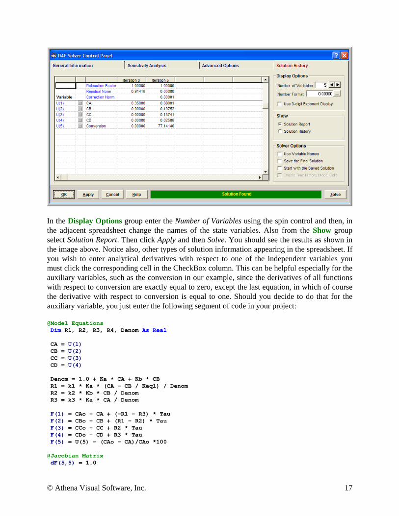
In the Display Options group enter the Number of Variables using the spin control and then, in the adjacent spreadsheet change the names of the state variables. Also from the Show group select Solution Report. Then click Apply and then Solve. You should see the results as shown in the image above. Notice also, other types of solution information appearing in the spreadsheet. If you wish to enter analytical derivatives with respect to one of the independent variables you must click the corresponding cell in the CheckBox column. This can be helpful especially for the auxiliary variables, such as the conversion in our example, since the derivatives of all functions with respect to conversion are exactly equal to zero, except the last equation, in which of course the derivative with respect to conversion is equal to one. Should you decide to do that for the auxiliary variable, you just enter the following segment of code in your project: @Model Equations Dim R1, R2, R3, R4, Denom As Real CA = U(1) CB = U(2) CC = U(3) CD = U(4) Denom = 1.0 + Ka * CA + Kb * CB R1 = k1 * Ka * (CA - CB / Keql) / Denom R2 = k2 * Kb * CB / Denom R3 = k3 * Ka * CA / Denom F(1) = CAo - CA + (-R1 - R3) * Tau F(2) = CBo - CB + (R1 - R2) * Tau F(3) = CCo - CC + R2 * Tau F(4) = CDo - CD + R3 * Tau F(5) = U(5) – (CAo – CA)/CAo *100 @Jacobian Matrix dF(5,5) = 1.0
© Athena Visual Software, Inc. 17