Asynchronous Evolution for Fully-Implicit and Semi...

Volume xx (200y), Number z, pp. 1–11

Asynchronous Evolution for Fully-Implicit and Semi-ImplicitTime Integration

Craig Schroeder1, Nipun Kwatra1, Wen Zheng1, Ron Fedkiw1,2

1Stanford University2Industrial Light+Magic

Figure 1: Twenty-four deformable objects fall into a bowl. Each body is evolved asynchronously with ε = .5.

AbstractWe propose a series of techniques for hybridizing implicit and semi-implicit time integration methods in a mannerthat retains much of the speed of the implicit method without sacrificing all of the higher quality vibrations oneobtains with methods that handle elastic forces explicitly. We propose our scheme in the context of asynchronousmethods, where different parts of the mesh are evolved at different time steps. Whereas traditional asynchronousmethods evolve each element independently, we partition all of our elements into two groups: one group evolved atthe frame rate using a fully implicit scheme, and another group which takes a number of substeps per frame usinga scheme that is implicit on damping forces and explicit on the elastic forces. This allows for a straightforwardcoupling between the implicit and semi-implicit methods at frame boundaries for added stability. As has beenstressed by various authors, asynchronous schemes take some of the pressure off of mesh generation, allowing timeevolution to remain efficient even in the face of sliver elements. Finally, we propose a force distributing projectionmethod which allows one to redistribute the forces felt on boundaries between implicit and semi-implicit regionsof the mesh in a manner that yields improved visual fidelity.

Categories and Subject Descriptors (according to ACM CCS): I.6.8 [Simulation and Modeling]: Types of Simulation—Animation

1. Introduction

Physically based simulation of deformable bodies has a longhistory in computer graphics. Since its early days, physical

submitted to COMPUTER GRAPHICS Forum (7/2011).

2 Shroeder et al. / Implicit Asynchronous Evolution

simulation has generally been limited by the small time stepsizes required for stability and the resulting computationalintensity of achieving realistic simulation. The early workof [BW98] changed this by popularizing implicit integra-tion and the conjugate gradient method within the commu-nity. This made it possible to take much larger time steps,making cloth simulation on reasonable mesh sizes practi-cal. With implicit integration techniques, stringent stabilityrestrictions were largely eliminated, and time steps of arbi-trary sizes could, in principle, be taken. In fact, one couldenvision taking time steps at the frame rate, which providesthe greatest opportunity for efficiency. This approach has al-ready received some attention, such as its recent successfulapplication to rigid bodies [SSF09].

Taking large time steps, however, has some significantshortcomings. Large time steps tend to introduce largeamounts of artificial damping into the simulation, and theycomplicate the problem of providing a robust collision re-sponse. The problem of artificial damping from large timesteps could in principle be overcome with with the useof symplectic integrators [], which can limit energy lossthrough the preservation of invariants. In practice, however,symplectic integrators require the solution of a nonlinearsystem. Unfortunately, this system might not converge iflarge time steps are taken, thus limiting its suitability to theproblem at hand.

The other complication, collision between bodies, tendsto be localized within a simulation. The rest of the simu-lation mesh is not limited by the small time steps requiredto provide a robust collision response. This suggests that atechnique based on asynchronous integration, where differ-ent parts of the mesh are permitted to take different time stepsizes, may be a promising compromise.

Asynchronous time integration has traditionally proven tobe most useful when the underlying method is fully explicit,where the size of the time step is stability limited (as opposedto accuracy limited) by both physical properties and meshquality. Although some attention has been paid to asyn-chronous schemes with implicit regions in other domains[GC01,GC03], previous asynchronous time integration tech-niques have tended to focus on explicit schemes, since ithas mainly been seen as a way of alleviating time step re-strictions due to numerical stability. We refer the reader to afew standard papers on the topic [Dan03,LMOW04,FDL08,HVS∗09]. The main idea of asynchronous integration is toevolve time forward, calculating forces in isolation on anelement-by-element basis, where each element is evaluatedat some future time based on its stability time step restric-tion. To make the determination of which element should beevaluated next more efficient, one typically uses a priorityqueue. Fully explicit methods and even semi-implicit meth-ods, where elastic forces are treated explicitly, such as thatof [BFA02, BMF03], which requires a time step restrictionfor elastic but not damping forces, both benefit from this sort

of time evolution model, since not all elements are subject totaking time steps at the frequency of the worst element in themesh. Larger, well-conditioned elements are allowed to takefewer time steps per frame.

When using a fully implicit method such as that of[BW98], one may take as big of a time step as visual fidelitywill allow (accuracy limited), without worrying about nu-merical stability. Therefore, an asynchronous priority queuebased on stability criteria no longer applies. However, thisnotion of visual fidelity does essentially bound the size ofthe time step. Although one might shrink the time step toincrease the accuracy, in turn increasing visual fidelity, thisleads to diminishing gains, because the implicit time stepsare more expensive than explicit ones. Therefore, makingthe implicit scheme computationally efficient usually meanslosing some accuracy. In a typical cloth simulation, loss ofaccuracy would lead to a loss of folds and wrinkles, see forexample [CK02] for a discussion of how buckling instabil-ities can be overdamped by numerical inaccuracies in im-plicit methods. We also refer the interested reader to [TPS08]for discussion of asynchronous integration in the context ofcloth simulation. Note that the amount at which one needto reduce the time step size to get sufficient accuracy de-pends a lot on the possible nonlinearity of the system. In thissense, cloth usually requires smaller time steps than solidobjects. Whereas the buckling instability makes things a bitmore complicated, we focus on the more direct problem ofthe loss of high frequency motion due to large time steps.We propose using asynchronous time integration in orderto alleviate this difficulty, evolving a portion of the meshat higher frequency in order to capture elastic vibrationalmodes while still treating the bulk of the mesh implicitlyfor the sake of computational efficiency. We also note thatcomputation efficiency of physics based simulations is ofgeneral interest to the graphics community, as can be seenby the interest that the problem of efficiency has receivedrecently [MTS07, Dru08, WST09].

Although [Dan03] does not address implicit asynchronoustime integration, they do advocate its use (as we do) for thesake of capturing high-frequency detail, even though it isnot needed for stability concerns. We further stress a sec-ond and very important application of asynchronous timeintegration for any method, which is collisions. Large timesteps can be problematic for any collision method and evenworse for self-collisions as in [BFA02], whereas smallertime steps ameliorate a large number of difficulties. Thus,regardless of whether time integration is treated explicitly,fully-implicitly, or semi-implicitly (where elastic forces aretreated explicitly and damping forces are treated implicitly),it can be quite important to treat elements undergoing colli-sions with smaller time steps.

Fully explicit schemes suffer from extremely small timestep restrictions from damping forces. These can be allevi-ated in a straightforward and efficient manner with a semi-


Shroeder et al. / Implicit Asynchronous Evolution 3

Semi-implicit Fully-implicit AsynchronousEfficiency Small time steps Large time steps Small time steps only where neededAccuracy Preserves high-frequency details Large damping, loss of details Preserves important details

Table 1: Comparison of the semi-implicit method, the fully implicit method and the asynchronous method.

implicit method which is explicit for nonlinear elastic forcesand implicit for linear and damping forces. We choose themethod of [SSIF09] (a small perturbation of [BMF03]) asour method of higher quality but smaller time step integra-tion scheme. This method produces high quality results atthe cost of adding computation time. We note that any othersemi-implicit or implicit scheme which treats the dampingforces implicitly could also be used. We use the method of[SLF08] for our fully-implicit scheme, as it is very similar toour semi-implicit scheme. As one would expect, greater nu-merical stability can be obtained by synchronizing the linearsystems for the damping in the semi-implicit scheme withthe linear system for the fully-implicit scheme. Therefore,we propose a bi-synchronous integration strategy, where thefully implicit scheme takes large time steps, while the semi-implicit scheme takes many smaller time steps which exactlyequal one time step of the fully implicit scheme. To stressefficiency and also to address problems that arise more gen-erally when transitioning to simulating with larger time stepsizes, we have decided to do our numerical experimentationand to present our examples with our implicit scheme takingtime steps at the frame rate. By doing this we are using theimplicit method in a way that uses the least computationalresources but also suffers greatly in in visual fidelity. Thishighlights the need for an method integrated with smallertime steps, which can capture the high frequency missing de-tails, making our proposed line of research more challengingbut also more effective. To help readers understand the con-tribution, a brief comparison between different methods hasbeen shown in Table 1.

We show examples that highlight basic collisions andself-collisions, complex geometry, and poor mesh quality.For each of these, we report on the results using the semi-implicit method along with its higher computational costsbut improved accuracy, the implicit method highlighting itsefficiency at the sake of extreme damping, and our newly-proposed bi-synchronous integration strategy. We highlightone of the drawbacks of asynchronous integration, which isthat larger elements have to wait longer for their forces to befelt, while smaller elements can push the mesh around freelywhile ignoring the forces from larger elements. There areways of ameliorating this to some extent using extrapolationof forces and other techniques, and we propose a scheme thatuses a projection method in the conjugate gradient solver inorder to distribute the forces from the nodes being evolvedat higher frequency to the nodes being evolved at lower fre-quency. Whereas this method does touch all particles at thefrequency of the explicit or semi-implicitly evolved parts of

the mesh, most particles are only touched with a simple pro-jection, saving on force evaluations and making the methodmore efficient. In the limit, (which we do not use) this is atype of rigidification of the fully-implicitly evolved nodesinto a kinematically deforming body - its frame is still fullytwo-way coupled and free to move unlike a traditional kine-matic body. We use this method away from the limit whereit helps to increase visual fidelity without adverse rigidifica-tion artifacts.

2. Related Work

Explicit asynchronous time integration has interested re-searchers for over three decades, beginning with [BM76,BYM79, Bel81], and continues to draw interest from thecommunity (see e.g. [CH08, Dan03] and the referencestherein). Asynchronous integrators have also been the sub-ject of stability and accuracy analysis (see e.g. [BS93,LMOW04, FDL08]). Asynchronous integration in the pres-ence of collisions has also received recent attention (see e.g.[TPS08, HVS∗09]).

There has also been work on explicit-implicit asyn-chronous evolution (see e.g. [GC01,GC03]). Unlike the con-text of explicit asynchronous integration, where stabilityconsiderations permit performance improvements for asyn-chronous evolution, the benefits sought from mixed explicit-implicit approaches are different. In the context of explicit-implicit integration, localized, highly nonlinear forces en-able efficiency gains to be achieved, since heavily nonlinearforces can be quite expensive to treat implicitly.

3. Synchronous Methods

3.1. Semi-Implicit Scheme

Our semi-implicit time integration scheme is based on thatof [SSIF09], which uses separate position and velocity up-dates to evolve bodies forward in time and takes the follow-ing basic form.

• vn+ 12 = vn + ∆t

2 a(tn+ 12 ,xn,vn+ 1

2 )

• xn+1 = xn +∆tvn+ 12

• vn+1 = vn +∆t a(tn+1,xn+1,vn+1)

The first step uses explicit evaluation of the elastic forcesgiven the current positions xn along with an implicit back-ward Euler update of the velocity component of the damp-ing forces. The second step uses this temporary velocity to



evolve the positions forward in time before the final step re-computes the velocity update, this time using the new posi-tions xn+1.

3.2. Fully-Implicit Scheme

Our fully-implicit scheme is based on that proposed in[SLF08], which is given by the scheme

• vn+ 12 = vn + ∆t

2 a(tn+ 12 ,xn + ∆t

2 vn+ 12 ,vn+ 1

2 )

• xn+1 = xn +∆tvn+ 12

• vn+1 = vn +∆t a(tn+1,xn+1,vn+1)

The only difference between this and our semi-implicitscheme is that xn is replaced by xn + ∆t

2 vn+ 12 , making that

update fully implicit. While this scheme is appealing sinceit is only a small modification to the semi-implicit schemeabove, it differs from that proposed in [SLF08] in that the fi-nal solution for velocity uses a backward Euler step insteadof a trapezoidal rule step. We note that using trapezoidal rulefor the second solution is not a good option for simulationswith large time step sizes, since it tends to cause period-twooscillations. Ironically, replacing their trapezoid rule with abackward Euler solution, a modification that would normallybe expected to enhance stability, makes the scheme only con-ditionally stable. This can be corrected by modifying the sec-ond solution to contain a predictive set of positions given byxn+2 = xn+1 +∆tvn+1, making it unconditionally stable. Theprecise scheme we use is

• vn+ 12 = vn + ∆t

2 a(tn+ 12 ,xn + ∆t

2 vn+ 12 ,vn+ 1

2 )

• xn+1 = xn +∆tvn+ 12

• vn+1 = vn +∆t a(tn+1,xn+1 +∆tvn+1,vn+1)

4. Asynchronous Methods

We derived and experimented with many implicit asyn-chronous schemes, and we present the best one along withsome of the more promising alternative approaches we con-sidered along the way. We also discuss advantages, limita-tions, and useful properties of each approach.

We divide our forces into two sets. The first set is evolvedsemi-implicitly at a smaller time step using the semi-implicitevolution described above. The second set is evolved fully-implicitly at the frame rate. In each case, the last semi-implicit step of each frame is fully coupled to the fully-implicit time step for that frame. (see Figure 2). The asyn-chronous scheme, as well as the the semi-implicit and fully-implicit schemes it is uses, has time time steps that take thegeneral form

• Compute v?

• Use v? to update positions to xn+1

• Compute vn+1

We consider the first two steps to be the position update andthe third step to be the velocity update.

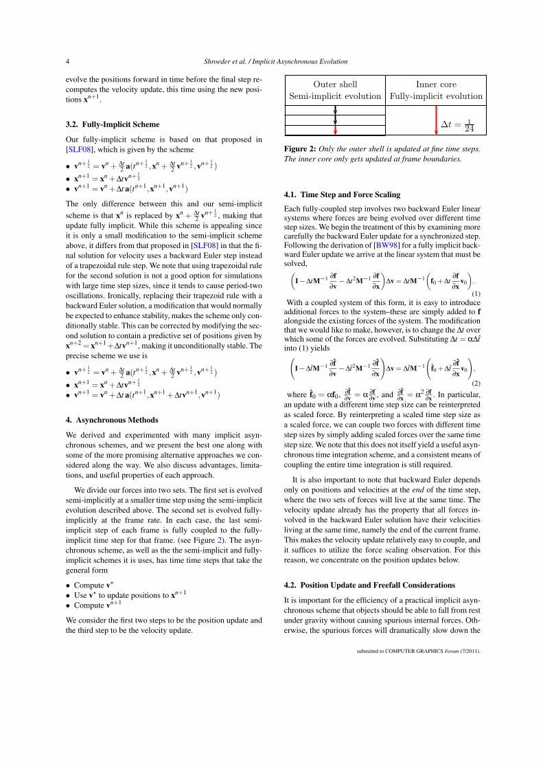
Outer shell Inner core

Semi-implicit evolution Fully-implicit evolution

∆t = 1

24

Figure 2: Only the outer shell is updated at fine time steps.The inner core only gets updated at frame boundaries.

4.1. Time Step and Force Scaling

Each fully-coupled step involves two backward Euler linearsystems where forces are being evolved over different timestep sizes. We begin the treatment of this by examining morecarefully the backward Euler update for a synchronized step.Following the derivation of [BW98] for a fully implicit back-ward Euler update we arrive at the linear system that must besolved,(

I−∆tM−1 ∂f∂v−∆t2M−1 ∂f

∂x

)∆v = ∆tM−1

(f0 + ∆t

∂f∂x

v0

).

(1)With a coupled system of this form, it is easy to introduce

additional forces to the system–these are simply added to falongside the existing forces of the system. The modificationthat we would like to make, however, is to change the ∆t overwhich some of the forces are evolved. Substituting ∆t = α∆tinto (1) yields(

I−∆tM−1 ∂f∂v−∆t2M−1 ∂f

∂x

)∆v = ∆tM−1

(f0 + ∆t

∂f∂x

v0

),

(2)

where f0 = αf0, ∂f∂v = α

∂f∂v , and ∂f

∂x = α2 ∂f

∂x . In particular,an update with a different time step size can be reinterpretedas scaled force. By reinterpreting a scaled time step size asa scaled force, we can couple two forces with different timestep sizes by simply adding scaled forces over the same timestep size. We note that this does not itself yield a useful asyn-chronous time integration scheme, and a consistent means ofcoupling the entire time integration is still required.

It is also important to note that backward Euler dependsonly on positions and velocities at the end of the time step,where the two sets of forces will live at the same time. Thevelocity update already has the property that all forces in-volved in the backward Euler solution have their velocitiesliving at the same time, namely the end of the current frame.This makes the velocity update relatively easy to couple, andit suffices to utilize the force scaling observation. For thisreason, we concentrate on the position updates below.

4.2. Position Update and Freefall Considerations

It is important for the efficiency of a practical implicit asyn-chronous scheme that objects should be able to fall from restunder gravity without causing spurious internal forces. Oth-erwise, the spurious forces will dramatically slow down the



solver and cause servere instability. One way for spuriousforces to occur is for particles to fall at slightly differentrates under gravity and experience elastic restorative forces,and the second is for particles to achieve different velocitiesin freefall and experience internal damping. Each of thesewould result in a significant slow down due to extra con-jugate gradient iterations during freefall. The force scalingapplies the correct amount of gravity in the velocity update,so that spurious damping forces are avoided. The positionupdate, however, requires more consideration.

We consider two approaches for avoiding positional er-rors in evolving gravity asynchronously. The first approachwe discuss involves making sure that the position update issecond order accurate, so that gravity is always evolved cor-rectly to floating point precision. We would tend to consideran approach following these general lines to be the most de-sirable. In practice, we were unable to overcome the poorerconditioning that our attempts at this approach produced.Instead, we present this approach as an example of how asuitable second order asynchronous position update can beachieved. That is, this approach works, but we were unableto make it efficient enough.

The second general approach we discuss is to abandon theidea of applying gravity asynchronously. This is clearly not asatisfying route for asynchronous evolution to follow goingforward. Rather, we note that applying gravity does not takea significant amount of time, and this compromise makes theresulting time integration scheme more efficient. We leave amore satisfying resolution of this problem to future work.

4.2.1. Second Order Positions

The first approach to a second order position update beginswith the observation that the position update

xn+1 = xn +∆t

(vn +vn+1

2

)(3)

is second order accurate. Let fE and fI be forces evaluatedat the time step size of semi-implicit and fully-implicit inte-grators, respectively. If we assume both sets of forces lackposition and velocity dependence and p semi-implicit stepsare taken for each fully-implicit step, then vn+1 can be writ-ten as

vn+1 = vn +M−1p

∑i=1

∆t ifE i +∆tM−1fI . (4)

Combining (3) and (4) we obtain

xn+1 = xn +∆tvn +∆t2

M−1p

∑i=1

∆t ifE i +∆t2

2M−1fI . (5)

To determine approximately how much a force that is ap-plied only every few time steps needs to be scaled for posi-tions to be evolved correctly, we make the assumption that

fI = 0, fE i = fE , and p∆t i = ∆t, then (see Appendix for de-tailed derivation)

xn+1 = xn+1− 1p +

∆tp

vn−1+ 1p +

∆t2

2p2 M−1fE

That is, in the last (pth) time step, one would apply the forcefE to the current x = xn+1− 1

p and v = vn−1+ 1p using the

current substep size. If fE i is not constant or fI 6= 0, taking asingle large step and taking many smaller steps are no longerequivalent. At this point, we make an approximation and ap-ply the explicit forces to the evolved state x and v. Addingback our implicit forces and dropping the assumption thatthe fE i is constant we obtain

xn+1 =x+∆t pv+∆t2

p

2M−1fE p +

∆t2

2M−1fI

=x+∆t pv+∆t2

p

2M−1(fE p +α

2fI) (6)

where α = (∆t/∆t p)2 is the correct scale for position update.

Note that (6) leads to a scaling factor of α2 for the implicit

elastic term rather than α as predicted by (2). That these twodo not match is the primary difficulty in choosing a positionupdate. Earlier in Section 4.1, we determined that a scalingfactor of α on forces is required to apply the correct amountof force during the velocity update, but it does not give ussecond order accurate positions.

A scheme produced using this position update has twodrawbacks. The first is that this α

2 scaling of the forces willproduce erroneous velocities when used in the first veloc-ity solution to calculate the velocities used in the positionupdate (as pointed out in Section 4.1). These erroneous ve-locities will be subject to other forces such as damping andthus not yield a correct steady state. The second drawback isthat the backward Euler evaluation is for the full ∆t, result-ing in a worse-conditioned and thus slower linear solution(we found the first linear system to require about twice thenumber of iterations as it would have had one used ∆t

2 as inthe semi-implicit scheme).

4.2.2. Avoiding Spurious Forces

The position update described above can be modified toavoid the mismatch in scales. In [BW98, SSIF09, SSF08],forces are recomputed after the conjugate gradients solution.In these papers, the results of the conjugate gradients solu-tion are used to explicitly recompute the forces that wereused in that solution. We utilize the same technique so thatthe proper scaling of α can be used inside the conjugate gra-dients solution while a scaling of α

2 can still be used in thesubsequent position update. The conjugate gradient solverproduces a solution v? to the following equation

v? =vn +∆tM−1 fE(xn,v?)+α∆tM−1 fI(xn +α∆tv?,v?).(7)



Instead of using this velocity in the position update, we usev? to explicitly re-evaluate fE and fI and then scale fI by α

2

to obtain the following velocity

vn+1 =vn+∆tM−1 fE(xn,v?)+α2∆tM−1 fI(xn+α∆tv?,v?).

(8)The full position update is (7), (8), and (3). This avoids theproblem of spurious forces in the solution in a straightfor-ward way. It does not address the extra computational costof solving the linear system across the full time step.

4.3. Asynchronous Integration Scheme

We can derive a more efficient scheme based on the idea ofevolving the velocity half way through the current time stepas in the semi-implicit case and then using it to update po-sitions. All positions and velocities are evolved forward intime even in the absence of forces on them so that positionscan all be updated with the step size ∆t. This amounts to ex-trapolating the behavior of the nodes that are evolved implic-itly forward through the time step. In the coupled time stepsthat synchronize the two methods, semi-implicit forces needto be evolved for time ∆t

2 so that the positions can be evolvedin a leap-frog fashion for a time step ∆t. The fully-implicitforces are evolved to the same point in time, which sincethey have been ignored for the entire frame means updatingthem for a time equal to ∆t f rame− ∆t

2 . This synchronizes thevelocities at a time that is ∆t

2 before the end of the frame.

This gives us the scaling factor α = 2∆t f rame−∆t∆t for use in

scaling forces. The computation of the half time velocitiesused in the position update becomes

vn+ 12 = vn +

∆t2

(aE(xn,vn+ 12 )+αaI(xn +α∆tvn+ 1

2 ,vn+ 12 ))

The main drawback of this scheme is that gravity must beapplied to all particles at each step to avoid spurious elasticforces during freefall. This scheme is what we used in ourexamples section. The coupled time steps for this schemeare

• vn+ 12 = vn + ∆t

2 (aE (xn,vn+ 12 )+ αaI(xn + α∆tvn+ 1

2 ,vn+ 12 ))

• xn+1 = xn +∆tvn+ 12

• vn+1 = vn +∆ta(xn+1 +∆tvn+1,vn+1)

where a indicates that the force scaling from Section 4.1 isapplied to fully implicit forces.

5. Force Distribution

The asynchronous scheme ignores the fully-implicit forcesduring most of the simulation and attempts to compensatefor them at frame boundaries. Consider a setup where theouter layer of tetrahedra have semi-implicit forces to resolvecollisions, and the interior has fully-implicit forces for ef-ficiency. During the semi-implicit steps, the sphere appearsto be hollow, held up only by the strength of the thin outerlayer of forces. Collisions cause the tetrahedra in contact

with the ground to be pushed into the interior, and the topof the sphere collapses into the sphere. To overcome thislimitation of asynchronous integration, we propose a novelmeans of distributing forces across regions of objects whoseforces are not being applied in the current time step. Notethat the force distribution operator only distributes the semi-implicit forces through the fully implicit regions when thefully implicit forces are not being applied. The rigid com-ponents within the semi-implicit regions are not affected.During coupled steps, the fully implicit forces are appliedas usual, and the fully-implicit and semi-implicit forces in-teract normally. Thus, while this approach modifies the ef-fective constitutive model, it does not override it entirely.

We begin by assuming that some subset of the particles arepart of a rigid body with mass m = ∑i mi and center of massc = m−1

∑i mixi. The particles can be described relative tothe center of mass by ri = xi−c, and the rigid body’s inertiatensor can be written as I = ∑i mir∗i r∗T

i , where r∗ representsthe cross product matrix of r. The total force on the rigidbody is f = ∑i fi, and the net torque is τ = ∑i r∗i fi, where firepresent forces in individual particles. The force and torquecause velocity changes per unit time of ∆v = m−1 f and∆ω = I−1

τ, and the corresponding velocity changes per unittime at a particular particle is ∆vi = ∆v+r∗T

∆ω. Finally, wecan compute forces that would need to have been applied atthese particles in the absence of the rigid body to producethe same result, which is fi = mi∆vi. The operator that takesfi and returns fi (obtained by combining all of these equa-tions) is a linear operator with very nice properties. It is arank-six mass-symmetric projection operator that preservesnet force and net torque, which is required for linear and an-gular momentum conservation. The six degrees of freedomnot projected out correspond to the three translational andthree rotational degrees of freedom of the rigid body.

This operator satisfies all of the properties necessary to beused as a projection in a conjugate gradient solver. As shownin the far right image in Figure 3 where the sphere has 21,528tetrahedra, this method constrains the particles subject tofully implicit forces to behave as a rigid body, except for thetemporary drift afforded by the fully coupled steps. This pro-vides an alternative method for simulating deformable bod-ies with rigid cores as proposed in [GOM∗06]. However,our aim is to simulate fully deformable bodies, not thosewith rigid cores, and thus we modify this method as follows.The first modification is that we apply the projections to theforces only, and not the velocities, which allows the particlesto retain relative motion. The second modification is that wedo not fully project the forces, as that would remove all ofthe non-bulk force and instead only partially project. Thiscan be accomplished by interpolating between the originalforces and the projected forces using a scalar ε, where ε = 0corresponds to doing nothing at all, and ε = 1 correspondsto using only the projected forces. Note that a more formalapproach to force distribution would be to model the wholeinterior of the body by a single coarse element of by a small



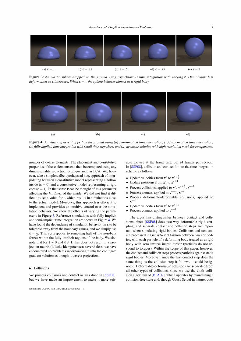
(a) ε = 0 (b) ε = .25 (c) ε = .5 (d) ε = .75 (e) ε = 1

Figure 3: An elastic sphere dropped on the ground using asynchronous time integration with varying ε. One obtains lessdeformation as ε increases. When ε = 1 the sphere behaves almost as a rigid body.

(a) (b) (c) (d)

Figure 4: An elastic sphere dropped on the ground using (a) semi-implicit time integration, (b) fully implicit time integration,(c) fully implicit time integration with small time step sizes, and (d) accurate solution with high resolution mesh for comparison.

number of coarse elements. The placement and constitutiveproperties of these elements can then be computed using anydimensionality reduction technique such as PCA. We, how-ever, take a simpler, albeit perhaps ad hoc, approach of inter-polating between a constitutive model representing a hollowinside (ε = 0) and a constitutive model representing a rigidcore (ε = 1). In that sense ε can be thought of as a parameteraffecting the hardness of the inside. We did not find it dif-ficult to set a value for ε which results in simulations closeto the actual model. Moreover, this approach is efficient toimplement and provides an intuitive control over the simu-lation behavior. We show the effects of varying the param-eter ε in Figure 3. Reference simulations with fully implicitand semi-implicit time integration are shown in Figure 4. Wehave found the dependence of simulation behavior on ε to betolerable away from the boundary values, and we simply useε = 1

2 . This corresponds to removing half of the non-bulkforces within the fully-implicit regions of the body. We alsonote that for ε 6= 0 and ε 6= 1, this does not result in a pro-jection matrix (it lacks idempotence); nevertheless, we haveencountered no problems incorporating it into the conjugategradient solution as though it were a projection.

6. Collisions

We process collisions and contact as was done in [SSF08],but we have made an improvement to make it more suit-

able for use at the frame rate, i.e. 24 frames per second.In [SSF08], collision and contact fit into the time integrationscheme as follows:

• Update velocities from vn to vn+ 12

• Update positions from xn to xn+1

• Process collisions, applied to vn, vn+ 12 , xn+1

• Process contact, applied to vn+ 12 , xn+1

• Process deformable-deformable collisions, applied toxn+1

• Update velocities from vn to vn+1

• Process contact, applied to vn+1

The algorithm distinguishes between contact and colli-sions, since [SSF08] does two-way deformable rigid cou-pling, and separate contact and collision steps are impor-tant when simulating rigid bodies. Collisions and contactsare processed in Gauss Seidel fashion between pairs of bod-ies, with each particle of a deforming body treated as a rigidbody with zero inverse inertia tensor (particles do not re-spond to torques). Within the scope of this paper, however,the contact and collision steps process particles against staticrigid bodies. Moreover, since the first contact step does thesame thing as the collision step it follows, it could be ig-nored. Deformable-deformable collisions are separated fromall other types of collisions, since we use the cloth colli-sion algorithm of [BFA02], which operates by maintaining acollision-free state and, though Gauss Seidel in nature, does



not lend itself easily to Gauss Seidel processing with othertypes of collisions.

The first six steps can be thought of as choosing the newpositions, and the last two steps can be thought of as choos-ing the new velocities. Because the collision algorithm of[SSF08] is designed to function properly in the context oftwo-way coupling, they are not able to take the much sim-pler collision approach used in [SSIF09] to handle collisionswith static rigid bodies. The time integration of [SSIF09] isable to directly fix both positions and velocities in a singlestep, and within the relatively narrow scope of this paper wecould have chosen to do the same. Instead, we stay within theconfines of the more general collision algorithm and addressits limitations.

Collisions with rigid bodies are processed by removingthe normal velocity from the particle and applying friction.The collision processing will force the normal relative veloc-ity between the particle and static bodies to be zero, so thatthe relative normal separation between them will not changeduring the time step. This results in a gap between objectsthat are otherwise in contact. That is, a particle falling to theground will stop just above the ground, separated from it by adistance of up to ∆tvrel , where vrel is the relative normal ve-locity. Since the particle is now at rest and above the ground(and thus not in contact with it), it will begin to fall undergravity until it hits the ground a second time and is stoppedcloser to the surface but still above it. This process allowsthe particle to approach the ground closer, until it is withina distance of 1

2 g∆t2 from the ground. Within this distance, itwill fall into the ground from rest in a single time step andbehave as though it were in contact. With time steps as largeas a frame, this initial collision gap can produce noticeableartifacts, since objects travel a noticeable distance in a singletime step.

We therefore propose a modification to the way collisionsare processed. The idea is to instead reduce the normal ve-locity so that positions will lie at the surface of the rigidbody after the time step and apply friction based on this im-pulse. This will produce a velocity whose normal compo-nent is still approaching. That is, the particle will still appearto be colliding after the position update, but the particle’sposition will be on the surface as desired. After the colli-sion step, three more steps will directly involve these mod-ified velocities and must each be considered. First, the ve-locities will be processed for contact immediately after thecollision step, and the modification to the collision responsemust be repeated here so that it is not undone. The secondstep that sees the modified velocity is the implicit velocityupdate. The third step to see the modified velocities is the fi-nal contact step, which must be handled carefully. This con-tact step must process the same pairs as collisions processedand should zero out relative normal velocity rather than tar-geting a position. After the time step has ended, the particleswill lie on the collision body surface with zero relative ve-

locity as desired. While this approach is rather subtle, it hasthe advantage of being applicable to the two-way coupledcontext of the original algorithm rather than being limited tothe narrower context of this paper.

For collisions between two deformable objects, we usethe collision algorithm of [BFA02]. Although this algorithmguarantees no interpenetration, it does not work well whentaking time steps as large as the frame rate. Since, our adap-tive asynchronous time integration takes small times stepson surface where collision occurs, it is quite useful for accu-rate resolution of self collisions. See Figures 5 (middle) and6 (left middle) for examples of failed collision resolution atlarge time steps. Note that one can also resolve this issue bycarefully designing their collision response methods like theimplicit contact handling method in [?].

7. Examples

In all our examples the surface elements are evolved semi-implicitly, while the internal elements are evolved fully im-plicitly. Figures 6 shows that we are able to handle morecomplicated geometry, even with self collisions. Observethat the fully implicit simulation in Figure 6 has collisionartifacts due to the frame rate collisions resolution, whereasthe asynchronous and semi-implicit simulations lack suchartifacts. We also show the extreme case ε = 1, which causesthe armadillo to behave almost like a rigid body wrapped in athin deformable mesh. It is still able to bend because we donot project velocities and because the coupled steps allowrelative motion of the interior particles. The effects of spa-tial refinement can be seen in Figure 7. Timings are shownin Table 2. In addition, the semi-implicit iteration is approx-imately half cheaper than the fully-implicit one.

We use the meshing algorithm of [MBTF03], which gen-erates well-conditioned elements in the interior of the mesh.The time step size in an explicit method is determinedby the time required for information to travel the lengthof the smallest feature in the mesh at the speed of soundin the material. This restriction is relaxed significantly forsemi-implicit methods and avoided entirely for fully-implicitmethods. Because of the quality and adaptivity of the mesh,the smallest elements, and therefore the shortest edges, oc-cur on the mesh’s surface. Since in all of our asynchronousexamples we evolve the surface elements semi-implicitly,

Figure 7: One sphere falling using meshes of various res-olutions: (left) 600 tetrahedra, (middle) 6,120 tetrahedra,(right) 21,528 tetrahedra.



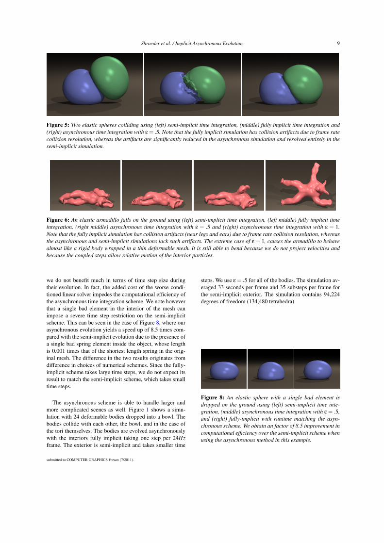
Figure 5: Two elastic spheres colliding using (left) semi-implicit time integration, (middle) fully implicit time integration and(right) asynchronous time integration with ε = .5. Note that the fully implicit simulation has collision artifacts due to frame ratecollision resolution, whereas the artifacts are significantly reduced in the asynchronous simulation and resolved entirely in thesemi-implicit simulation.

Figure 6: An elastic armadillo falls on the ground using (left) semi-implicit time integration, (left middle) fully implicit timeintegration, (right middle) asynchronous time integration with ε = .5 and (right) asynchronous time integration with ε = 1.Note that the fully implicit simulation has collision artifacts (near legs and ears) due to frame rate collision resolution, whereasthe asynchronous and semi-implicit simulations lack such artifacts. The extreme case of ε = 1, causes the armadillo to behavealmost like a rigid body wrapped in a thin deformable mesh. It is still able to bend because we do not project velocities andbecause the coupled steps allow relative motion of the interior particles.

we do not benefit much in terms of time step size duringtheir evolution. In fact, the added cost of the worse condi-tioned linear solver impedes the computational efficiency ofthe asynchronous time integration scheme. We note howeverthat a single bad element in the interior of the mesh canimpose a severe time step restriction on the semi-implicitscheme. This can be seen in the case of Figure 8, where ourasynchronous evolution yields a speed up of 8.5 times com-pared with the semi-implicit evolution due to the presence ofa single bad spring element inside the object, whose lengthis 0.001 times that of the shortest length spring in the orig-inal mesh. The difference in the two results originates fromdifference in choices of numerical schemes. Since the fully-implicit scheme takes large time steps, we do not expect itsresult to match the semi-implicit scheme, which takes smalltime steps.

The asynchronous scheme is able to handle larger andmore complicated scenes as well. Figure 1 shows a simu-lation with 24 deformable bodies dropped into a bowl. Thebodies collide with each other, the bowl, and in the case ofthe tori themselves. The bodies are evolved asynchronouslywith the interiors fully implicit taking one step per 24Hzframe. The exterior is semi-implicit and takes smaller time

steps. We use ε = .5 for all of the bodies. The simulation av-eraged 33 seconds per frame and 35 substeps per frame forthe semi-implicit exterior. The simulation contains 94,224degrees of freedom (134,480 tetrahedra).

Figure 8: An elastic sphere with a single bad element isdropped on the ground using (left) semi-implicit time inte-gration, (middle) asynchronous time integration with ε = .5,and (right) fully-implicit with runtime matching the asyn-chronous scheme. We obtain an factor of 8.5 improvement incomputational efficiency over the semi-implicit scheme whenusing the asynchronous method in this example.



Test namesemi-implicit fully-implicit asynchronous (seconds/frame)(seconds/frame) (seconds/frame) ε = 0 ε = .25 ε = .5 ε = .75 ε = 1

1 sphere 0.87 0.47 1.2 1.18 1.16 1.08 0.842 spheres 3.31 1.47 4.29 4.38 4.31 4.05 3.09Armadillo 3.55 1.03 3.58 3.69 3.51 3.45 3.371 sphere with

13.24 0.8 1.61 1.91 1.54 1.26 1.26a single bad element

Table 2: Wall clock times comparing the semi-implicit method, the fully implicit method and the asynchronous method.

8. Conclusion and Future Work

We present an implicit asynchronous time integrationscheme that evolves one set of forces semi-implicitly at asmall time step size and another set of forces fully implicitlywith a larger time step size to allow better collision reso-lution and visual fidelity. We use a novel force distributionmethod to avoid interior collapse due to asynchronous evolu-tion. Our time integration scheme works well with collisionsand self collisions, and it can achieve an order of magnitudespeed improvement for meshes that contain bad elements.

Although we only consider two regions, a semi-implicitregion and a fully-implicit, one is not limited to only tworegions. In fact, there could be many semi-implicit regions,each one categorized to flow at some finer time step, or onemight also consider using an explicit, fully asynchronousmethod within the semi-implicit region so that each elementis applied in the most efficient fashion. Another area we havenot adequately explored is different means of choosing re-gions for different time steps.

We note that we did not achieve the efficiency gains thatwe were expecting. One of the main reasons for this is thattaking time steps of twice the size does not accelerate theruntime by a factor of two. Although the time steps arelarger, the cost of each time step increases. This is becausethe matrix upon which conjugate gradient is acting has theform A = I−∆tM−1 ∂f

∂v −∆t2M−1 ∂f∂x . As ∆t → 0, A → I,

which greatly improves the conditioning of the problem andaccelerates the rate of convergence of the conjugate gradientalgorithm. In particular, the effect on conditioning becomesa very significant factor when ∆t is on the order of the framerate. This is why the fully implicit simulations, running atthe frame rate, are only a small factor more efficient thanthe semi-implicit simulations, which run with over ten timesas many time steps. This in turn severely limits the gainsthat asynchronous evolution is able to provide. One avenuefor improving upon our asynchronous scheme is to addressthe conditioning problems caused by the fully implicit forcesapplied over the large ∆t.

The force distribution scheme was necessary because themesh tends to collapse or experience other undesirable be-haviors when being evolved with the interior forces dis-abled. It seems likely that the asynchronous time integrationscheme itself could be modified in a way that avoids this

limitation without the need for adding additional forces. Weleave this for future work.

While our results leave room for improvement, we feelthat this is a promising avenue for future research. We alsofeel that many of the ideas and observations we have madealong the way may be helpful to others that are interested inpursuing asynchronous integration.

Acknowledgement

Research supported in part by a Packard Foundation Fellow-ship, an Okawa Foundation Research Grant, ONR N0014-06-1-0393, ONR N00014-05-1-0479 for a computing clus-ter, NIH U54-GM072970, and NSF CCF-0541148. C.S. wassupported in part by a Stanford Graduate Fellowship.

References[Bel81] BELYTSCHKO T.: Partitioned and adaptive algorithms

for explicit time integration. Nonlinear Finite Element Anal. inStruct. Mech. (1981), 572–584.

[BFA02] BRIDSON R., FEDKIW R., ANDERSON J.: Robust treat-ment of collisions, contact and friction for cloth animation. ACMTrans. Graph. 21, 3 (2002), 594–603.

[BM76] BELYTSCHKO T., MULLEN R.: Mesh partitions ofexplicit-implicit time integration. Formulations and Computa-tional Algorithms in Finite Element Analysis, K. Bathe, J. Odenand W. Wunderlich, eds., MIT Press, Cambridge, Mass (1976),673–690.

[BMF03] BRIDSON R., MARINO S., FEDKIW R.: Simulation ofclothing with folds and wrinkles. In Proc. of the 2003 ACM SIG-GRAPH/Eurographics Symp. on Comput. Anim. (2003), pp. 28–36.

[BS93] BIESIADECKI J., SKEEL R.: Dangers of multiple timestep methods. J. of Comp. Phys. 109 (1993), 318–328.

[BW98] BARAFF D., WITKIN A.: Large steps in cloth simula-tion. In ACM SIGGRAPH 98 (1998), ACM Press/ACM SIG-GRAPH, pp. 43–54.

[BYM79] BELYTSCHKO T., YEN H., MULLEN R.: Mixed meth-ods for time integration. Comp. Meth. in Appl. Mech. and Engng.17, 18 (1979), 259–275.

[CH08] CASADEI F., HALLEUX J.: Binary spatial partitioningof the central-difference time integration scheme for explicit fasttransient dynamics. International Journal Numerical Methods inEngineering (2008).

[CK02] CHOI K.-J., KO H.-S.: Stable but responsive cloth. ACMTrans. Graph. (SIGGRAPH Proc.) 21 (2002), 604–611.



[Dan03] DANIEL W.: A partial velocity approach to subcyclingstructural dynamics. Comp. Meth. Appl. Mech. Engng. 192(2003), 375–94.

[Dru08] DRUMWRIGHT E.: A fast and stable penalty method forrigid body simulation. IEEE Trans. Viz. Comput. Graph. 14, 1(2008), 231–240.

[FDL08] FONG W., DARVE E., LEW A.: Stability of asyn-chronous variational integrators. J. Comput. Phys. 227 (2008),8367–94.

[GC01] GRAVOUIL A., COMBESCURE A.: Multi-time-stepexplicit-implicit method for non-linear structural dynamics. Intl.J. for Numer. Meth. in Engng. 50, 1 (2001), 199–225.

[GC03] GRAVOUIL A., COMBESCURE A.: Multi-time-step andtwo-scale domain decomposition method for non-linear struc-tural dynamics. Intl. J. for Numer. Meth. in Engng. 58, 10 (2003),1545–1569.

[GOM∗06] GALOPPO N., OTADUY M. A., MECKLENBURG P.,GROSS M., LIN M. C.: Fast simulation of deformable mod-els in contact using dynamic deformation textures. In Proc.of the ACM SIGGRAPH/Eurographics Symp. on Comput. Anim.(2006), pp. 73–82.

[HVS∗09] HARMON D., VOUGA E., SMITH B., TAMSTORF R.,GRINSPUN E.: Asynchronous contact mechanics. In ACM SIG-GRAPH 2009 (2009), ACM Press/ACM SIGGRAPH, pp. 1–12.

[LMOW04] LEW A., MARSDEN J., ORTIZ M., WEST M.: Vari-ational time integrators. Int. J. Num. Meth. Eng. 60 (2004), 153–212.

[MBTF03] MOLINO N., BRIDSON R., TERAN J., FEDKIW R.:A crystalline, red green strategy for meshing highly deformableobjects with tetrahedra. In 12th Int. Meshing Roundtable (2003),pp. 103–114.

[MTS07] MOUSTAKAS K., TZOVARAS D., STRINTZIS M.: SQ-Map: Efficient layered collision detection and haptic rendering.IEEE Trans. Viz. Comput. Graph. 13, 1 (2007), 80–93.

[SLF08] SELLE A., LENTINE M., FEDKIW R.: A mass springmodel for hair simulation. ACM Transactions on Graphics 27, 3(Aug. 2008), 64.1–64.11.

[SSF08] SHINAR T., SCHROEDER C., FEDKIW R.: Two-waycoupling of rigid and deformable bodies. In SCA ’08: Proceed-ings of the 2008 ACM SIGGRAPH/Eurographics symposium onComputer animation (2008), pp. 95–103.

[SSF09] SU J., SCHROEDER C., FEDKIW R.: Energy stabilityand fracture for frame rate rigid body simulations. In Proceedingsof the 2009 ACM SIGGRAPH/Eurographics Symp. on Comput.Anim. (2009), pp. 155–164.

[SSIF09] SELLE A., SU J., IRVING G., FEDKIW R.: Robusthigh-resolution cloth using parallelism, history-based collisions,and accurate friction. IEEE Trans. on Vis. and Comput. Graph.(2009), 339–350.

[TPS08] THOMASZEWSKI B., PABST S., STRASSER W.: Asyn-chronous cloth simulation. In CGI Proc. 2008 (2008).

[WST09] WICKE M., STANTON M., TREUILLE A.: Modularbases for fluid dynamics. ACM Trans. Graph. 28, 3 (2009), 1–8.

Appendix

Derivation of Second Order Positions

Recall that the second order position update looks like (5).

If we let fI = 0, fE i = fE , and p∆t i = ∆t, then

vn+ kp =vn+ k−1

p +∆tp

M−1fE

=vn +k∆tp

M−1fE

xn+ kp =xn+ k−1

p +∆t2p

(vn+ k−1

p +vn+ kp

)=xn+ k−1

p +∆tp

vn +∆t2

p2

(k− 1

2

)M−1fE

=xn +k∆tp

vn +k2

∆t2

2p2 M−1fE

xn+1 =xn +∆tvn +∆t2

M−1p

∑i=1

∆t ifE i

=xn +∆tvn +∆t2

2M−1fE

=xn+1− 1p +

∆tp

vn +(2p−1)∆t2

2p2 M−1fE

=xn+1− 1p +

∆tp

vn−1+ 1p +

∆t2

2p2 M−1fE


Asynchronous Evolution for Fully-Implicit and Semi...

Documents

Transcript of Asynchronous Evolution for Fully-Implicit and Semi...