Asymmetric Information and Adverse Selection.

Based on Akerlof (1970).

A Simple Labor Market Model.

Many identical firms.

Firms risk neutral (Maximize expected profit).

Firms price taking.

Price of output =1.

Production uses only labor.

Constant marginal productivity of labor: θ

Productivity θ differs across workers.

θ ∈ [θ, θ].

0 ≤ θ < θ <∞

Distribution of workers’ productivity: distribution func-tion F (θ).

F (θ) = proportion of workers with productivity of at most θ.

Assume: F is non-degenerate (at least two types of pro-ductivity in the population of workers).

Finite number (measure) of workers.

A worker can work at home or at a firm.

If a worker of type (i.e., productivity) θ works at homeshe earns r(θ).

[We refer to r(θ) as "reservation wage" or opportunitycost of accepting employment of a worker of type θ].

A worker of type θ accepts employment if and only if herwage ≥ r(θ).

Benchmark: Full information (productivity of each workeris publicly observable).

Competitive equilibrium.

A distinct equilibrium wage w∗(θ) for each θ.

Price taking agents in the labor market.

wage = marginal product of labor.

w∗(θ) = θ

Firms earn zero profit (constant returns technology).

Set of workers that are employed in the firms in equilib-rium are those with productivity in the set:

{θ : r(θ) ≤ θ}.

This equilibrium is Pareto optimal: every worker who ismore productive at home then in the firms is employedat home and the rest work in the firms.

No other allocation can increase total surplus generated.

Asymmetric Information.

Workers’ productivity not observed by firms.

Competitive equilibrium:

One wage w for all worker types.

Set of worker types willing to work in the firms at wagerate w :

Θ(w) = {θ : r(θ) ≤ w}.so that the realized average productivity of workers em-ployed at wage w is:

E[θ | θ ∈ Θ(w)].

If a firm believes that the expected productivity of workersis μ, then its demand for labor at wage w is

0, if w > μ

[0,∞), if w = μ

∞, if w < μ.

For market clearing with positive employment in firms weneed:

w = μ

Rational expectations: expectations are fulfilled (expectedproductivity = average productivity of workers that workin firms):

μ = E[θ | θ ∈ Θ(w)].

So, equilibrium wage w∗ satisfies the equation :

w∗ = E{θ | r(θ) ≤ w∗}.In this equilibrium, the set of workers finding employment:

Θ∗(w∗) = {θ : r(θ) ≤ w∗}.

Note:

If no worker accepts employment the average productivityE[θ | θ ∈ Θ(w)] is not well defined as Θ(w) is a setof measure zero. In this case we take μ = E[θ], theunconditional expectation.

* Competitive equilibrium may be Pareto inefficient.

Suppose r(θ) = r, ∀θ ∈ [θ, θ].

In that case, the set of workers willing to work in in firms

Θ(w) = [θ, θ], if w ≥ r

= φ, if w < r.

So, the expected productivity of workers in a competi-tive equilibrium is E(θ), the unconditional expectationof random variable θ.

This does not depend on the wage.

If E(θ) ≥ r, then in equilibrium

w∗ = E(θ)

and all workers are employed in firms.

If E(θ) < r,no worker is employed in firms.

There is possibility of Pareto inefficiency in both situa-tions.

For example, if

θ < r < E(θ)

then workers whose productivity θ ∈ [θ, r) are employedin firms (attracted by the high wage that exceeds theirproductivity) but actually would be more socially produc-tive at home.

On the other hand, if

E(θ) < r < θ

then workers of type θ ∈ (r, θ] are employed at homethough they would be more productive at work.

Both problems arise because employers cannot distinguishtypes of workers and price discriminate; they pay accord-ing to the population average.

This inefficiency is a consequence of asymmetric informa-tion.

Note: if it is socially optimal for all workers to work inthe firms i.e., r < θ or for all workers to work at homeθ < r, then competitive equilibrium is Pareto optimal.

But a potentially more serious problem for the marketarises when r(θ) varies with θ.

In that case, the type of workers willing to work at acertain wage and their average productivity can vary withthe wage.

Adverse Selection:

Adverse selection occurs when an informed individual’strading decision depends on her unobservable character-istics (type) in such a way that it adversely affects theuninformed agents in the market.

Here: relatively less productive workers are willing to ac-cept employment in firms at any wage.

This can lead to unraveling of the market.

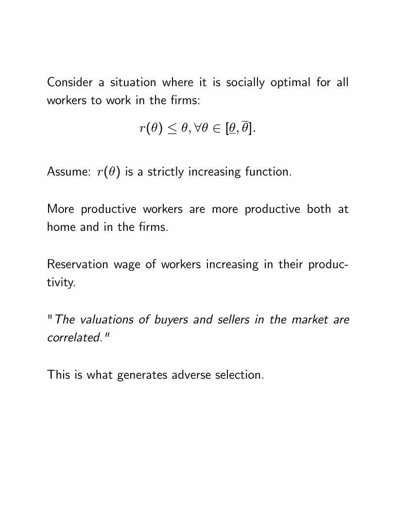
Consider a situation where it is socially optimal for allworkers to work in the firms:

r(θ) ≤ θ,∀θ ∈ [θ, θ].

Assume: r(θ) is a strictly increasing function.

More productive workers are more productive both athome and in the firms.

Reservation wage of workers increasing in their produc-tivity.

"The valuations of buyers and sellers in the market arecorrelated."

This is what generates adverse selection.

Assume: F (.) has a density function f(θ) > 0 on [θ, θ].

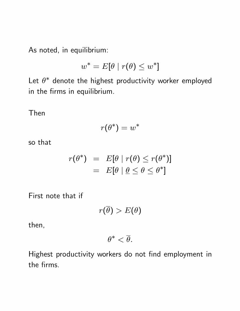
As noted, in equilibrium:

w∗ = E[θ | r(θ) ≤ w∗]

Let θ∗ denote the highest productivity worker employedin the firms in equilibrium.

Then

r(θ∗) = w∗

so that

r(θ∗) = E[θ | r(θ) ≤ r(θ∗)]= E[θ | θ ≤ θ ≤ θ∗]

First note that if

r(θ) > E(θ)

then,

θ∗ < θ.

Highest productivity workers do not find employment inthe firms.

For best quality workers to employment in firms, the wagewould have to be high enough - but in that case all work-ers of lower productivity would also find it optimal to beemployed.

The average productivity of all workers is not good enoughfor firms to offer a wage that attracts the best workers.

So, in equilibrium, only lower productivity workers (θ ≤θ∗) are employed by firms.

Bad workers drive good workers out of the market. (Gre-sham’s Law).

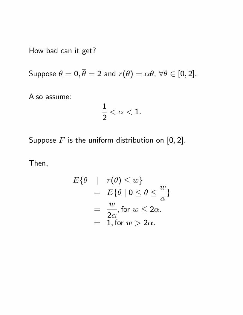
How bad can it get?

Suppose θ = 0, θ = 2 and r(θ) = αθ, ∀θ ∈ [0, 2].

Also assume:1

2< α < 1.

Suppose F is the uniform distribution on [0, 2].

Then,

E{θ | r(θ) ≤ w}= E{θ | 0 ≤ θ ≤ w

α}

=w

2α, for w ≤ 2α.

= 1, for w > 2α.

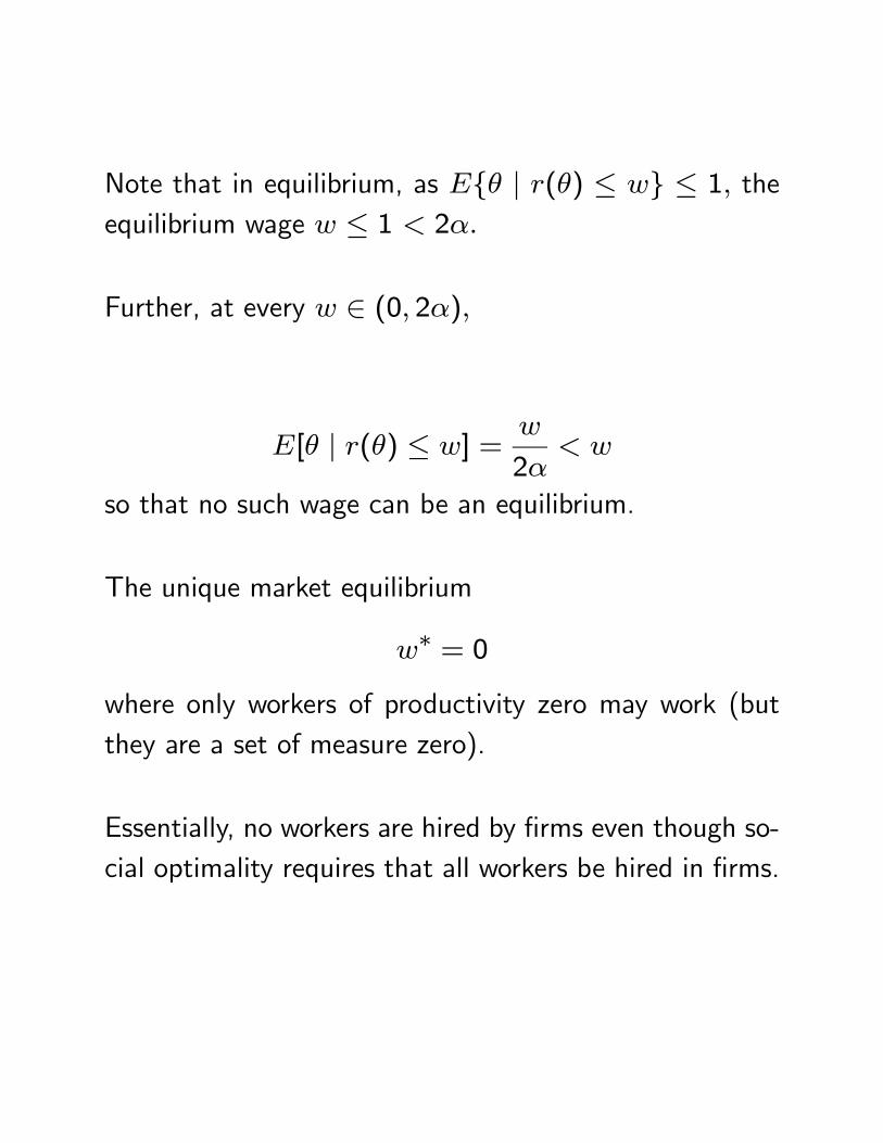
Note that in equilibrium, as E{θ | r(θ) ≤ w} ≤ 1, theequilibrium wage w ≤ 1 < 2α.

Further, at every w ∈ (0, 2α),

E[θ | r(θ) ≤ w] =w

2α< w

so that no such wage can be an equilibrium.

The unique market equilibrium

w∗ = 0

where only workers of productivity zero may work (butthey are a set of measure zero).

Essentially, no workers are hired by firms even though so-cial optimality requires that all workers be hired in firms.

Other possibilities:

Multiple equilibria that are Pareto ranked.

Equilibria with higher wage - bigger range of θ employed,workers earn greater surplus.

(Firms always earn zero profit).

Signaling.

Spence (1973,1974).

What mechanisms can allow firms to distinguish betweenworkers?

Agents with private information can choose actions thatenrich the information structure of uninformed agents -more particularly, allow the latter to make rational infer-ence about the "types" of informed agents.

Direct revelation of types through a "test" or certificationby experts may not always be feasible.

Need for sophisticated signaling mechanisms.

Modify the labor market model to a strategic model.

2 firms

1 worker

Worker of two possible types with constant marginal pro-ductivity: θH, θL

θH > θL > 0

Priors:

Pr[θ = θH] = λ ∈ (0, 1)Pr[θ = θL] = 1− λ ∈ (0, 1)

Before entering job market a worker can get some edu-cation.

Amount of education received is publicly observable.

Assume: Education does not affect a worker’s productiv-ity.

Education here is a pure information signaling device.

Cost of obtaining education level e for a type θ worker:c(e, θ).

Assume:c(e, θ) is a twice continuously differentiable func-tion with

c(0, θ) = 0,

ce(e, θ) > 0, cee(e, θ) > 0, cθ(e, θ) < 0,∀e > 0

ceθ(e, θ) < 0.

This implies: Both total and marginal cost of educationare lower for high productivity workers.

Let u(w, e | θ) denote utility of type θ worker whochooses education level e and receives wage w.

Let

u(w, e | θ) = w − c(e, θ).

Note: Single Crossing Condition. The indifference curvesof type θH and type θL workers in the (w, e) space crossonly once and at the point of intersection the indifferencecurve of the θL type worker is steeper.

[Indifference curve

w − c(e, θ) = K

with slope:

dw

de= ce(e, θ)

and this is decreasing in θ as ceθ < 0.]

As before, a worker of type θ can earn r(θ) by workingat home.

Assume:

r(θH) = r(θL) = 0

Note: if there is no signaling, firms first make wage offersand then the worker chooses whether to accept and whichone, then the unique equilibrium in that case is that bothfirms offer wage (Bertrand competition)

w∗ = E(θ).

The market equilibrium is Pareto efficient.

We use this to illustrate the peculiar inefficiencies thatsignaling generates.

Signaling Game:

1. Nature determines type of worker using a probabilitydistribution that assumes value θH with probability λ andθL with probability 1− λ. This move is not observed byfirms.

2. Worker chooses education level (signal) conditional onher realized type: e(θH), e(θL).

3. Both firms observe the chosen education level e of theworker and then choose wages.

4. Worker decides whether to accept one of the two offers& if so, which one.

Strategy of firm i: wi(e).

Perfect Bayesian Equilibrium: A set of strategies and abelief function μ(e) ∈ [0, 1] giving the firms’ commonprobability assessment that the worker is of type θH afterobserving education level e where:

(i) The worker’s strategy is optimal given the firms’ strate-gies

(ii) The belief function μ(e) is derived from the worker’sstategy using Bayes’ rule wherever possible

(iii) The firms’ wage offers following each e constitutea Nash equilibrium of the simultaneous move wage offergame in which the probability that the worker is of typeθH is μ(e).

[This PBE is equivalent to a Sequential Eqm].

Work backwards.

The last stage of worker’s decision is easy - worker willaccept the higher wage offer and will randomize acrossthe two firms (say, with equal probability) if they bothmake the same wage offer.

Now we go to third stage.

Firms have observed e and attached posterior probabilityμ(e) to the event that the worker is of type θH.

So for both firms, the (conditional) expected productivityof worker (conditional on e):

μ(e)θH + (1− μ(e))θL.

Therefore, Bertrand like competition leads to a uniqueNE in this simultaneous move wage offer game:

w1(e) = w2(e) = w(e) = μ(e)θH + (1− μ(e))θL.

Note w(e) ∈ [θL, θH].

Separating Equilibria:

Let e∗(θ) denote equilibrium strategy of worker andw∗(e)the firms’equilibrium wage schedule.

* In any separating PBE, each worker type receives awage equal to her productivity level i.e.,

w∗(e∗(θL)) = θL

w∗(e∗(θH)) = θH.

Why? Because beliefs of firms’ must be consistent withequilibrium strategies.

* In any separating PBE, a low-ability worker chooseszero education i.e., e∗(θL) = 0.

Why? Low ability worker can never lose on the wage bychoosing zero education, the worst he can be thought ofis that he is low ability and that still gets him the samewage as he could get in any separating equilibrium; inaddition he saves on the cost of education.

Constructing a separating PBE:

Set

e∗(θL) = 0, w∗(0) = w∗(e∗(θL)) = θL.

A low ability worker then earns utility θL.

Now, consider the wage θH that must be received by thehigh ability worker.

As θH > θL, the low ability worker would love to pretendto be a high ability worker.

To take away this incentive, we need to set the educationlevel required to signal high ability type sufficiently high.

Let ee > 0 be defined by

θL = θH − c(ee, θL).As long as e∗(θH) ≥ ee, the low ability worker has noincentive imitate the high ability worker.

As c(ee, θL) > c(ee, θH),θH − c(ee, θH) > θL

so that a high ability worker has no incentive to imitate alow ability worker if e∗(θH) = ee or even slightly higher.

Set

e∗(θH) = ee, w∗(ee) = w∗(e∗(θH)) = θH.

We now need to ensure that the way w∗(e) function be-haves outside the points {0, ee}, makes it optimal for bothtypes of workers to not deviate from their assigned edu-cation levels.

Of course, at each e, w∗(e) must equal the expectedproductivity of worker with that education level given thebeliefs μ(e) of the firms.

PBE: no restriction on how beliefs can be assigned offthe equilibrium path in the signaling game.

So, we have a wide degree of freedom in choosing w∗(e)on (0, ee).

For example, consider beliefs:

μ∗(e) = 0, if e < ee.μ∗(e) = 1, if e ≥ ee.

and the wage schedule:

w∗(e) = θL, if e < ee.w∗(e) = θH, if e ≥ ee.

Easy to check that neither type worker wants to deviate.

Can sustain same PBE with a variety of off-equilibriumbeliefs.

Other separating PBE where e∗(θH) > ee.Separating PBE with lower value of e∗(θH) Pareto dom-inates separating PBE with higher value of e∗(θH).

Same wages, same output, more education cost.

Separating PBE with e∗(θH) = ee Pareto dominates allother separating PBE.

Compare separating PBE with signaling to outcome whenthere is no possibility of signaling (and no education costeither).

In latter case, both types of worker employed at wageE(θ) = λθH + (1− λ)θL.

If we allow for signaling, in the separating PBE, workerof type t employed at wage θt.

Low type worker worse off.

High type worker may or may not be better off dependingon whether:

E(θ) S θH − c(e∗(θH), H)

Observe: as λ changes, the set of separating PBE is un-affected.

As λ → 1,the cost of education (signaling cost) in anyseparating PBE remains high, and nearly all workers aregetting educated to signal type even though there arevery few low types.

Pooling Equilibria:

e∗(θH) = e∗(θL) = e∗.

Belief on the equilibrium path must be:

μ∗(e∗) = λ

so that

w∗(e∗) = λθH + (1− λ)θL = E(θ).

Let e0 be defined by:

θL = E(θ)− c(e0, L)

* Any e ∈ [0, e0] can be sustained as w∗(e) = θL,ife < e0 in a pooling PBE.

Beliefs:

μ∗(e) = 0, if e < e0.μ∗(e) = λ, if e = e0.μ∗(e) = 1, if e > e0.

and the wage schedule:

w∗(e) = θL, if e < e0.w∗(e) = E(θ), if e = e0

w∗(e) = θH, if e > e0.

Pooling equilibria with higher e∗ Pareto dominated byone with lower e∗.

Pooling equilibrium with e∗ = 0 generates same outcomeas a competitive outcome with no possibility of signaling.

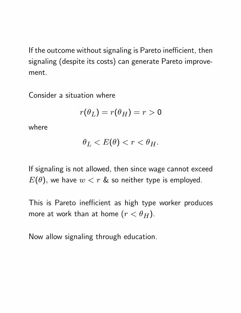
If the outcome without signaling is Pareto inefficient, thensignaling (despite its costs) can generate Pareto improve-ment.

Consider a situation where

r(θL) = r(θH) = r > 0

where

θL < E(θ) < r < θH.

If signaling is not allowed, then since wage cannot exceedE(θ), we have w < r & so neither type is employed.

This is Pareto inefficient as high type worker producesmore at work than at home (r < θH).

Now allow signaling through education.

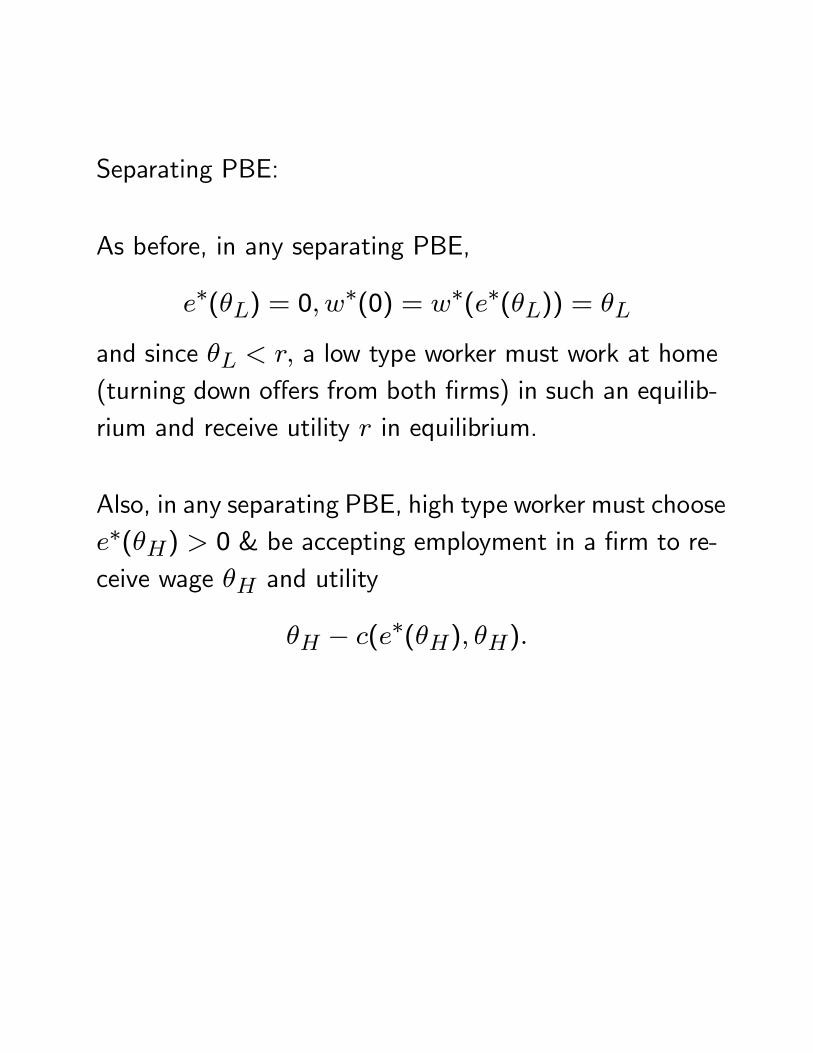
Separating PBE:

As before, in any separating PBE,

e∗(θL) = 0, w∗(0) = w∗(e∗(θL)) = θL

and since θL < r, a low type worker must work at home(turning down offers from both firms) in such an equilib-rium and receive utility r in equilibrium.

Also, in any separating PBE, high type worker must choosee∗(θH) > 0 & be accepting employment in a firm to re-ceive wage θH and utility

θH − c(e∗(θH), θH).

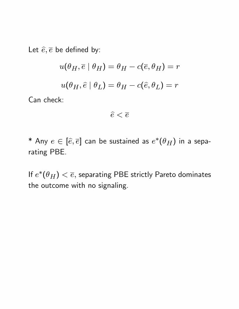
Let be, e be defined by:u(θH, e | θH) = θH − c(e, θH) = r

u(θH, be | θL) = θH − c(be, θL) = r

Can check:

be < e

* Any e ∈ [be, e] can be sustained as e∗(θH) in a sepa-rating PBE.

If e∗(θH) < e, separating PBE strictly Pareto dominatesthe outcome with no signaling.

Asymmetric information develops between parties aftercontracting.

Contract has to be designed anticipating the difficultiescaused by this.

Important class of such problems:

Principal- Agent Problems:

One individual (principal) hires another individual (agent)to take some actions for him.

Two kinds of informational problems can arise post-contract:

(i) Those arising from actions of agent being hidden fromor unobservable by principal (moral hazard)

(ii) Those arising from some information possessed oracquired by the agent being hidden the principal.

A Model of Moral Hazard.

Principal: Owner of a firm.

Agent: Manager.

Owner hires manager for a single project.

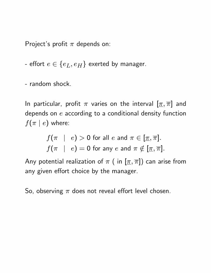
Project’s profit π depends on:

- effort e ∈ {eL, eH} exerted by manager.

- random shock.

In particular, profit π varies on the interval [π, π] anddepends on e according to a conditional density functionf(π | e) where:

f(π | e) > 0 for all e and π ∈ [π, π].f(π | e) = 0 for any e and π /∈ [π, π].

Any potential realization of π ( in [π, π]) can arise fromany given effort choice by the manager.

So, observing π does not reveal effort level chosen.

Let F (π | e) be the conditional distribution functionassociated with f.

Assume: The conditional distribution of profit given efforteH has a strict first order stochastic dominance over thatcorresponding to effort level eL.

F (π | eH) ≤ F (π | eL), ∀π ∈ [π, π]F (π | eH) < F (π | eL), ∀π ∈ Π ⊂ [π, π]

where Π is an open subset of [π, π].

Thus:

E[π | eH] > E[π | eL].

Manager: expected utility maximizer with Bernoulli util-ity function:

u(w, e) = v(w)− g(e)

where v is twice continuously differentiable in w on R+with

v0 > 0, v” ≤ 0and

g(eH) > g(eL).

- prefers more income to less

- weakly risk-averse over income lotteries

- dislikes high effort.

Reservation utility of agent: u > 0.

Manager accepts a contract if and only if it gives him anexpected utility of at least u.

Owner: risk neutral and maximizes expected profit net ofpayment made to manager.

Assume: If manager does not accept offer, then ownergets zero

Assume: owner finds it profitable to make the manger anoffer that he will accept

(i.e., its not the case that the owner makes an offer know-ing that it will be rejected).

First Best (Full information):

Effort is Observable.

Contract specifies the manager’s effort e ∈ {eH, eL} andwage payment as a function of observed profits w(π).

The first best optimal contract:

maxe∈{eH,eL},w(π)

πZπ

(π −w(π))f(π | e)dπ

s.t.

πZπ

v(w(π))f(π | e)dπ − g(e) ≥ u

Solve it in two stages:

1. For any e, what is the optimal w(π) so that themanager still accepts the contract?

2. What is the optimal e?

First, consider (1).

Given e, the problem

maxw(π)

πZπ

(π −w(π))f(π | e)dπ

s.t.

πZπ

v(w(π))f(π | e)dπ − g(e) ≥ u

reduces to

minw(π(

πZπ

w(π)f(π | e)dπ

s.t.

πZπ

v(w(π))f(π | e)dπ − g(e) ≥ u

The constraint is always binding (otherwise the manager’swages can always be lowered while giving him his reser-vation utility).

L =

πZπ

w(π)f(π | e)dπ

+γ[

πZπ

v(w(π))f(π | e)dπ − g(e)− u]

=

πZπ

(w(π) + γv(w(π))]f(π | e)dπ

−g(e)− u

Taking the first order condition with respect to the man-ager’s wage at each level of π :

[−1 + γv0(w(π))]f(π | e) = 0which implies:

v0(w(π)) = 1

γ

If v” < 0, then this implies that for all π ∈ [π, π],

w(π) = v0−1(1γ), a constant

so that the unique optimal compensation scheme is onethat is constant valued for all π i.e., a fixed wage scheme.

The risk neutral owner should fully insure the risk aversemanager against any risk in his income stream.

The fixed wage w∗(e) satisfies:

v(w∗(e))− g(e) = u.

As g(eH) > g(eL), the manager’ wage is higher if thecontract gets him to choose eH rather than eL.

If manager is risk neutral:

Suppose v(w) = w.

Any compensation scheme w(π) that gives the manageran expected wage payment equal to u+ g(e) is optimal.

This includes the fixed wage scheme w∗(e) describedabove.

As for optimal choice of e :

maxe∈{eH,eL}

πZπ

πf(π | e)dπ − v−1(u+ g(e)).

The optimal fixed wage scheme follows.

The above is the unique first best scheme if v” < 0.

It is a first best scheme if v” = 0 i.e., manager is riskneutral.

Second Best: Optimal Contract When Effort is NotObservable.

Contract cannot specify an effort level.

Use w(π) to indirectly induce the right kind of effort.

Case of Risk-Neutral Manager.

Assume v(w) = w.

If effort was observable, firm owner would want the man-ager to exert effort e∗ that solves:

maxe∈{eH,eL}

πZπ

πf(π | e)dπ − (u+ g(e))

and owner’s net profit in this first best world is:

πZπ

πf(π | e∗)dπ − (u+ g(e∗))

while the manager receives an utility of u.

We now claim that even when effort is not observable,the owner can offer a contract that gives the owner thesame payoff (and the manager the same utility) as underfull information.

This is the optimal contract.

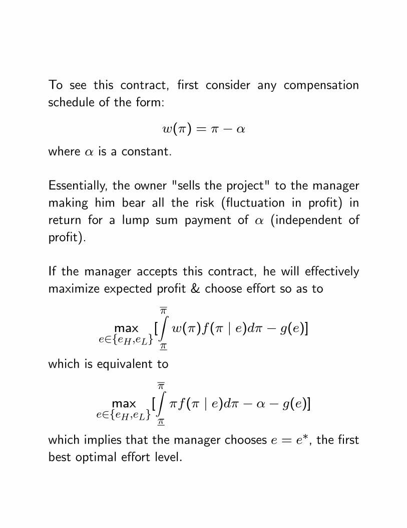
To see this contract, first consider any compensationschedule of the form:

w(π) = π − α

where α is a constant.

Essentially, the owner "sells the project" to the managermaking him bear all the risk (fluctuation in profit) inreturn for a lump sum payment of α (independent ofprofit).

If the manager accepts this contract, he will effectivelymaximize expected profit & choose effort so as to

maxe∈{eH,eL}

[

πZπ

w(π)f(π | e)dπ − g(e)]

which is equivalent to

maxe∈{eH,eL}

[

πZπ

πf(π | e)dπ − α− g(e)]

which implies that the manager chooses e = e∗, the firstbest optimal effort level.

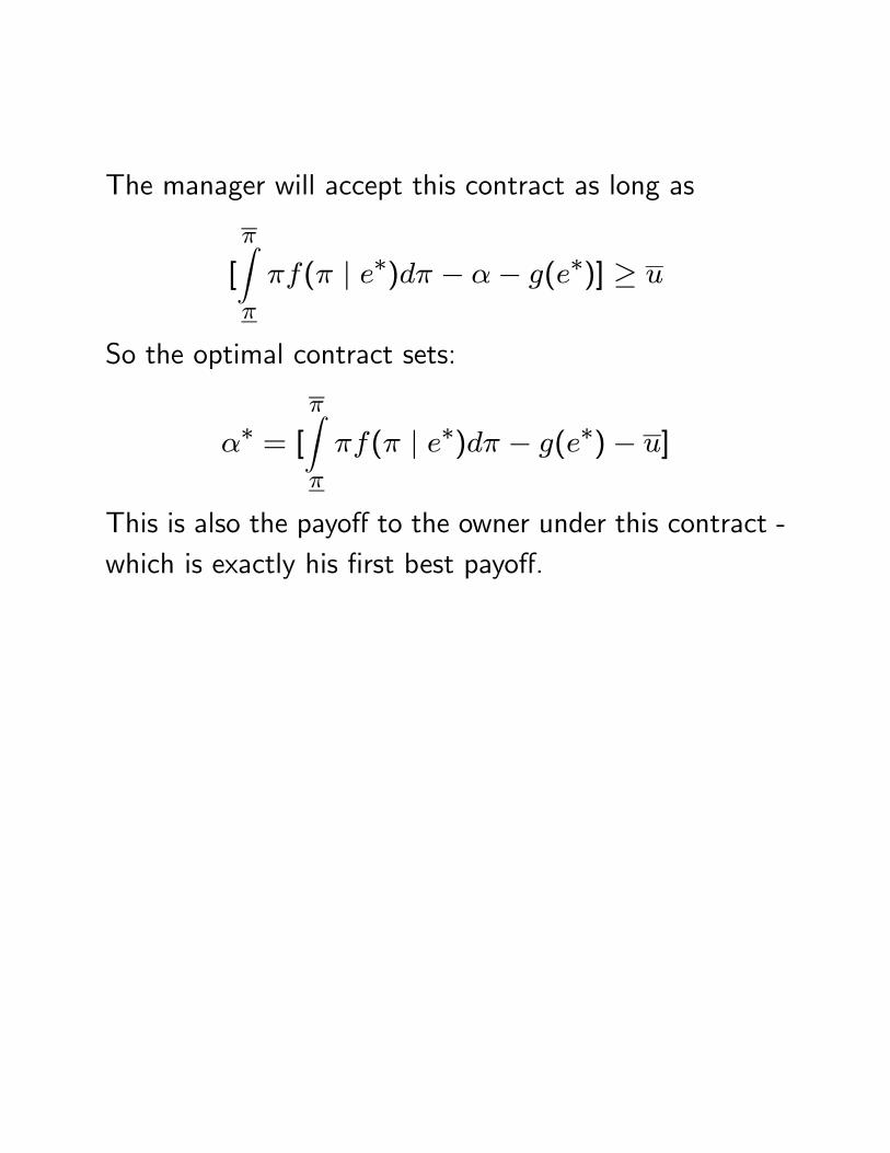
The manager will accept this contract as long as

[

πZπ

πf(π | e∗)dπ − α− g(e∗)] ≥ u

So the optimal contract sets:

α∗ = [πZπ

πf(π | e∗)dπ − g(e∗)− u]

This is also the payoff to the owner under this contract -which is exactly his first best payoff.

When both principal and agent are risk neutral, the prob-lem of risk sharing disappears.

Manager can be given incentive to bear the full marginalreturn from his effort.

Efficient.

This kind of a scheme becomes problematic if :

(1) Agent is Risk averse: manager requires additionalrisk premium to take the entire fluctuation in profit onhimself.

(2) Agent has limited liability: does not have assets tobear hugely negative profit realizations.

Risk-averse Manager.

To provide incentive for high effort, we need the man-ager’s compensation to vary with profit - we need themanager to bear some risk.

But then, compensating him for the risk is costly.

So, there is a trade-off.

Leads to inefficiency.

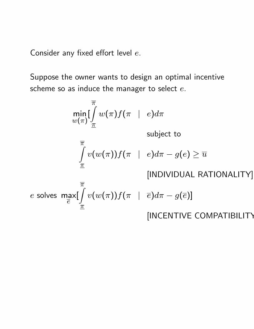
Consider any fixed effort level e.

Suppose the owner wants to design an optimal incentivescheme so as induce the manager to select e.

minw(π)

[

πZπ

w(π)f(π | e)dπ

subject toπZπ

v(w(π))f(π | e)dπ − g(e) ≥ u

[INDIVIDUAL RATIONALITY]

e solves maxe[

πZπ

v(w(π))f(π | e)dπ − g(e)]

[INCENTIVE COMPATIBILITY

If e = eL, then the optimal scheme for the owner isto offer the same fixed wage it would offer if he wantedagent to choose eL in the first best case viz., w∗e =

v−1(u+ g(eL)).

With this scheme, agent chooses eL even if effort is notobservable as it has lower disutility.

This is an optimal way of getting the agent to exert thiseffort, as the owner can never do better than in the firstbest world.

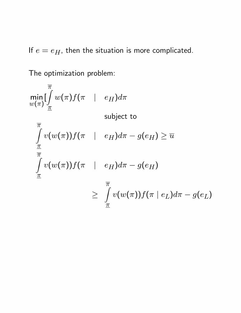
If e = eH, then the situation is more complicated.

The optimization problem:

minw(π)

[

πZπ

w(π)f(π | eH)dπ

subject toπZπ

v(w(π))f(π | eH)dπ − g(eH) ≥ u

πZπ

v(w(π))f(π | eH)dπ − g(eH)

≥πZπ

v(w(π))f(π | eL)dπ − g(eL)

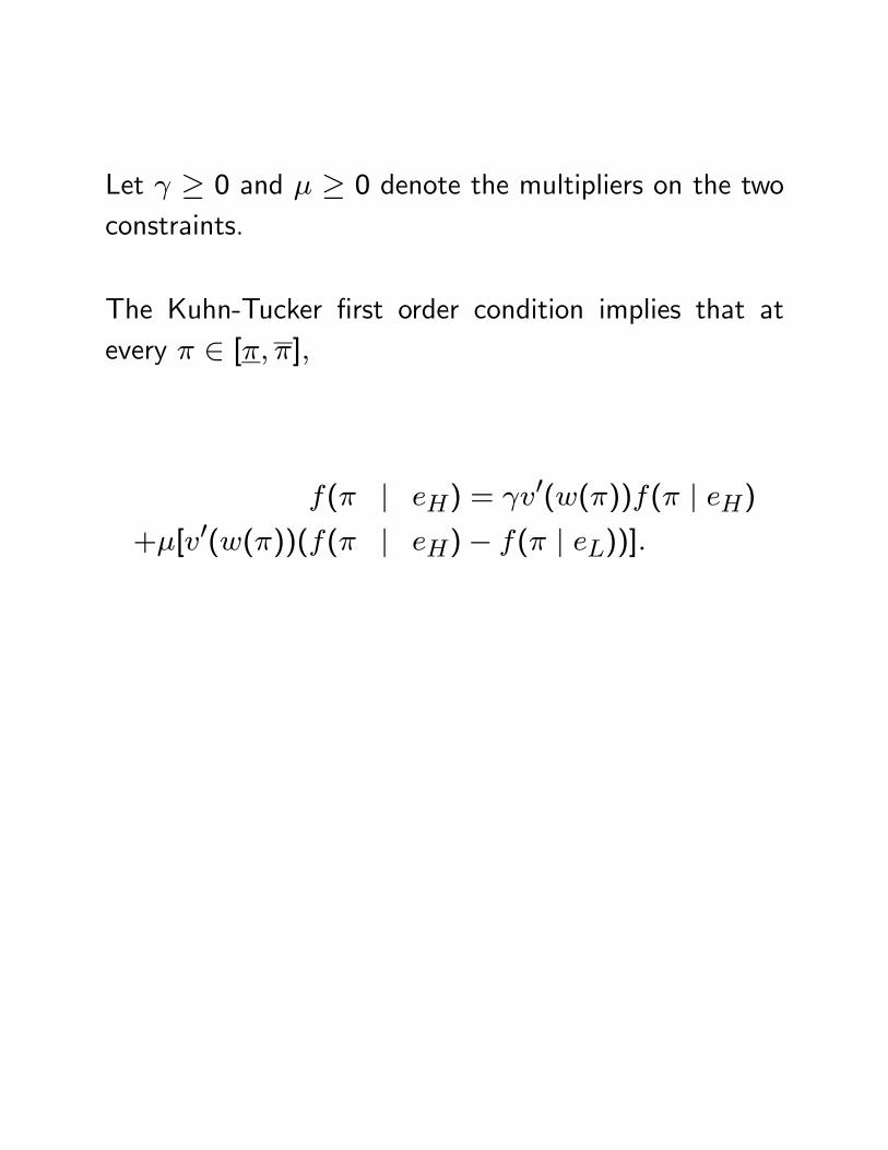
Let γ ≥ 0 and μ ≥ 0 denote the multipliers on the twoconstraints.

The Kuhn-Tucker first order condition implies that atevery π ∈ [π, π],

f(π | eH) = γv0(w(π))f(π | eH)+μ[v0(w(π))(f(π | eH)− f(π | eL))].

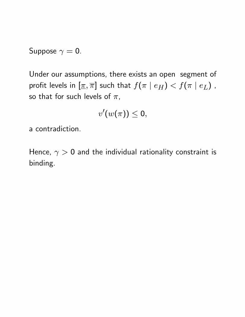
Suppose γ = 0.

Under our assumptions, there exists an open segment ofprofit levels in [π, π] such that f(π | eH) < f(π | eL) ,so that for such levels of π,

v0(w(π)) ≤ 0,a contradiction.

Hence, γ > 0 and the individual rationality constraint isbinding.

Suppose μ = 0. Then:

γv0(w(π)) = 1,∀π ∈ [π, π]so that the optimal scheme would be a fixed wage scheme.

However, under any fixed wage scheme, the managerwould always choose eL as it yields lower disutilty andso it contradicts the hypothesis that the scheme imple-ments eH.

Hence, μ > 0 and the incentive compatibility constraintis binding.

The FOC can be re-written as:

1

v0(w(π))= γ + μ[1− f(π | eL)

f(π | eH)].

[ f(π|eL)f(π|eH)] is the ratio of the "likelihood" of getting profitlevel π when effort level is eL to that when effort level iseH.

The condition says that the wages should vary with profitaccording to changes in the likelihood ratio.

Monotone Likelihood Ratio Property: f(π|eL)f(π|eH) is decreas-

ing in π.

This is not implied by first order stochastic dominance.

If MLRP holds, the optimal w(π) is increasing in π.

Otherwise, it may be non-monotonic.

Finally, recall that in the full information case where effortis observable, a fixed wage payment could implement eHand that wage was w∗eH = v−1(u+ g(eH)).

With effort unobserved, the optimal scheme w(π) forimplementing eH is not a fixed wage scheme and since

E[v(w(π))]− g(eH) = u

it follows from Jensen’s inequality that

v(E(w(π))) > E[v(w(π))] = g(eH) + u

so that

E(w(π)) > v−1(u+ g(eH)) = w∗eH.

For the manager to get reservation utility u with a riskycompensation scheme, the mean wage must be higher (tocompensate for the variance) than in the risk-less fixedwage case.

This immediately implies that if the owner tries to imple-ment eH he will be making higher expected payment tothe manager than under observability of effort.

His own expected profit from implementing eH must belower than under observability.

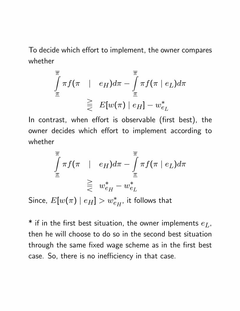
To decide which effort to implement, the owner compareswhether

πZπ

πf(π | eH)dπ −πZπ

πf(π | eL)dπ

T E[w(π) | eH]−w∗eLIn contrast, when effort is observable (first best), theowner decides which effort to implement according towhether

πZπ

πf(π | eH)dπ −πZπ

πf(π | eL)dπ

T w∗eH −w∗eLSince, E[w(π) | eH] > w∗eH , it follows that

* if in the first best situation, the owner implements eL,then he will choose to do so in the second best situationthrough the same fixed wage scheme as in the first bestcase. So, there is no inefficiency in that case.

* if in the first best situation, the owner implements eH,then there are two possibilities:

(a) he will still find it optimal to do so in the second bestcase; in which case he will choose a non-constant wagescheme w(π) where E[w(π) | eH] > w∗eH and will makeless expected profit than in the first best case.

(b) he will no longer find it optimal to implement eHin the second best case and will choose the fixed wagew∗eL to implement eL earning the same level of expectedprofit as he would have earned in the first best case ifhe chosen to implement eL instead of eH.

Since eH is the optimal effort level in the first best case,he earns less expected profit than in the first best case.

In both (a) and (b), the worker will still earns the sameexpected utility as in the first best case viz., u.

Thus, there is inefficiency resulting from non-observabilityand the second best payoff is lower for the owner.