arX

iv:a

stro

-ph/

0605

581v

3 1

6 Ja

n 20

07

Parameterization of γ, e± and Neutrino Spectra Produced by p − p

Interaction in Astronomical Environment

Tuneyoshi Kamae1, Niklas Karlsson2, Tsunefumi Mizuno3, Toshinori Abe4, Tatsumi Koi

Stanford Linear Accelerator Center, Menlo Park, CA 94025

kamae@slac.stanford.edu

ABSTRACT

We present the yield and spectra of stable secondary particles (γ, e±, νe, νe,

νµ, and νµ) of p−p interaction in parameterized formulae to facilitate calculations

involving them in astronomical environments. The formulae are derived from the

up-to-date p−p interaction model by Kamae et al. (2005), which incorporates the

logarithmically rising inelastic cross section, the diffraction dissociation process,

and the Feynman scaling violation. To improve fidelity to experimental data

in lower energies, two baryon resonance contributions have been added: one

representing ∆(1232) and the other representing multiple resonances around 1600

MeV/c2. The parametrized formulae predict that all secondary particle spectra

be harder by about 0.05 in power-law indices than that of the incident proton and

their inclusive cross-sections be larger than those predicted by p − p interaction

models based on the Feynman scaling.

Subject headings: cosmic rays — galaxies: jets — gamma-rays: theory — ISM:

general — neutrinos — supernovae: general

1. Introduction

Gamma-ray emission due to neutral pions produced by proton-proton interaction has

long been predicted from the Galactic ridge, supernova remnants (SNRs), active galactic nu-

cleus (AGN) jets, and other astronomical sites (Hayakawa 1969; Stecker 1971; Murthy & Wolfendale

1Also with Kavli Institute for Particle Astrophysics and Cosmology, Stanford University, Menlo Park,

CA 94025

2Visiting scientist from Royal Institute of Technology, SE-10044 Stockholm, Sweden

3Present address: Department of Physics, Hiroshima University, Higashi-Hiroshima, Japan 739-8511

4Present address: Department of Physics, University of Tokyo, Tokyo, Japan 113-0033

– 2 –

1986; Schonfelder 2001; Schlickeiser 2002; Aharonian 2004; Aharonian et al. 2004). High en-

ergy neutrinos produced by p−p interaction in AGN jets will soon be detected with large-scale

neutrino detectors that are under construction (Halzen 2005). Spectra of these gamma-rays,

neutrinos, and other secondaries depend heavily on the incident proton spectrum, which

is unknown and needs to be derived, in almost all cases, from the observed spectra them-

selves. Such analyses often involve iterative calculations with many trial proton spectra.

The parameterized model presented here is aimed to improve accuracy of such calculations.

Among the secondaries of p − p interaction in astronomical environment, gamma-rays

have been best studied. The p-p interaction is one of the two dominant gamma-ray emission

mechanisms in the sub-GeV to multi-TeV range, the other being Compton up-scattering of

low energy photons by high energy electrons. Gamma-rays in this energy range have been

detected from pulsars, the Galactic Ridge, SNRs, blazars and other source categories (Stecker

1971; Murthy & Wolfendale 1986; Ong 1998; Schonfelder 2001; Weekes 2003; Aharonian

2004).

High energy gamma-rays from AGN jets are interpreted as mostly due to the inverse

Compton up-scattering of low-energy photons by multi-TeV electrons. Observed radio and

X-ray spectra match those of synchrotron radiation by these electrons. Synchronicity in

variability between the observed X-ray and gamma-ray fluxes has given strong support for

the inverse Compton up-scattering scenario (Ong 1998; Schonfelder 2001; Schlickeiser 2002;

Aharonian 2004). For some AGN jets, the above scenario does not work well, and p −

p interaction has been proposed as an alternative mechanism (Mucke & Protheroe 2001;

Mucke et al. 2003; Bottcher & Reimer 2004).

High energy gamma-rays detected by COS-B and EGRET from the Galactic Ridge, on

the other hand, are interpreted as predominantly due to neutral pions produced by interac-

tion of protons and nuclei with the interstellar matter (ISM; Stecker 1973; Strong et al. 1978,

1982, 2000; Stephens & Badhwar 1981; Mayer-Hasselwander et al. 1982; Bloemen et al. 1984;

Bloemen 1985; Dermer 1986a; Stecker 1990; Hunter et al. 1997; Mori 1997; Stanev 2004).

The measured gamma-ray flux and spectral shape (Hunter et al. 1997) have been viewed as

the key attestation to this interpretation. It is also known that inverse Compton scattering

contributes significantly to the Galactic Ridge gamma-ray emission (Murthy & Wolfendale

1986; Strong et al. 2000; Schonfelder 2001).

In the past two years, several SNRs, including RX J1713-3946 and RX J0852-4622,

have been imaged in the TeV band with an angular resolution around 0.1◦ by H.E.S.S.

(Aharonian et al. 2004b,c; Aharonian 2005). A smooth featureless spectrum, suggestive of

synchrotron radiation by multi-TeV electrons, has been detected in the X-ray band from RX

J1713-3946 (Koyama et al. 1997; Slane et al. 1999; Uchiyama et al. 2003) and RX J0852-

– 3 –

4622 (Tsunemi et al. 2000; Iyudin et al. 2005). The measured TeV gamma-ray fluxes and

spectra, however, do not agree well with those predicted by the inverse Compton scenario

(see, e.g., the analysis in Uchiyama et al. (2003)). Several authors have proposed that

the TeV gamma-rays are possibly due to interaction of accelerated protons with the ISM

(Berezhko & Volk 2000; Enomoto et al. 2002; Aharonian 2004; Katagiri et al. 2005).

Higher precision data are expected, in the GeV range, from GLAST Large Area Tele-

scope (GLAST-LAT 2005)1 and, in the TeV range, from the upgraded Air Cherenkov Tele-

scopes (Aharonian et al. 2004): they will soon test applicability of the inverse Compton up-

scattering and the proton interaction with ISM for various astronomical gamma-ray sources.

In many objects, secondary electrons and positrons may produce fluxes of hard X-rays and

low-energy gamma-rays detectable with high-sensitivity instruments aboard Integral, Swift,

Suzaku, and NuSTAR.2 The formulae given here will give fluxes and spectra of these sec-

ondary particles for arbitrary incident proton spectrum.

This work is an extension of that by Kamae et al. (2005), where up-to-date knowl-

edge of the π0 yield in the p − p inelastic interaction has been used to predict the Galac-

tic diffuse gamma-ray emission. The authors have found that past calculations (Stecker

1970, 1973, 1990; Strong et al. 1978; Stephens & Badhwar 1981; Dermer 1986a,b; Mori 1997;

Strong et al. 2000) had left out the diffractive interaction and the Feynman scaling violation

in the non-diffractive inelastic interaction. Another important finding by them is that most

previous calculations have assumed an energy-independent p − p inelastic cross-section of

about 24 mb for Tp ≫ 10 GeV, whereas recent experimental data have established a log-

arithmic increase with the incident proton energy. Updating these shortfalls has changed

the prediction on the gamma-ray spectrum in the GeV band significantly: the gamma-ray

power-law index is harder than that of the incident proton; and the GeV−TeV gamma-ray

flux is significantly larger than that predicted on the constant cross-section and Feynman

scaling (Kamae et al. 2005). The model by Kamae et al. (2005) will hereafter be referred to

as model A.

Model A does not model p − p interaction accurately near the pion production thresh-

old. To improve prediction of gamma-rays, electrons, and positrons produced near the pion

production threshold, two baryon resonance excitation components have bee added to model

A: ∆(1232), representing the ∆ resonance, and res(1600), representing resonances around

1GLAST Large Area Telescope, http://www-glast.stanford.edu.

2See INTEGRAL Web site, http://sci.esa.int/esaMI/Integral, the NuSTAR Web site,

http://www.nustar.caltech.edu, the Suzaku Web site http://www.isas.jaxa.jp/e/enterp/missions/astro-e2,

and the Swift Web site, http://swift.gsfc.nasa.gov/docs/swift.

– 4 –

1600 MeV/c2. We note here that ∆(1232) is the most prominent and lightest Baryon res-

onance excited in p − p interaction. It has a mass of 1.232 GeV/c2 and a width of about

0.12 GeV/c2, and decays to a nucleon (proton or neutron) and a pion (π+,0,−). The other

resonance, res(1600), is assumed to decay to a nucleon and two pions. Introduction of these

contributions have necessitated adjustment of the model A at lower energies as described

below. The readjusted model will be referred to as the “readjusted model A”.

The parameterized model presented here exhibits all features of model A at higher

energies (proton kinetic energy, Tp > 3 GeV) and reproduces experimental data down to the

pion production threshold. The inclusive gamma-ray and neutrino cross-section formulae

can be used to predict their yields and spectra for a wide range of incident proton spectrum.

Formulae for electrons and positrons predict sub-TeV to multi-TeV secondary electrons and

positrons supplied by p − p interaction. We note that space-borne experiments such as

PAMELA3 will soon measure the electron and positron spectra in the sub-TeV energy range,

where the secondaries of p−p interaction may become comparable to the primary components

(Muller 2001; Stephens 2001; DuVernois et al. 2001).

Due to paucity of experimental data and widely accepted modeling, we have not param-

eterized inclusive secondary cross-sections for α − p nor p−He nor α−He interactions. We

note that α-particles are known to make up about 7% by number of cosmic-rays observed

near the Earth (Schlickeiser 2002) and that He to make up ∼ 10% by number of interstellar

gas. The total non p − p contribution is comparable to that of p − p contribution. The

α-particle and He nucleus can be regarded, to a good approximation, as four independent

protons beyond the resonance region (Tp > 3 GeV): the error introduced is expected to be

less than 10% for high energy light secondary particles (Kamae et al. 2005).

Inclusion of α-particle as projectile and He nuclei as targets will change the positron-

electron ratio significantly (about 10 − 15%) as discussed below. Fermi motion of nucleons

and multiple nucleonic interactions in the nucleus are known to significantly affect pion

production near the threshold and in the resonance region (Tp < 3 GeV; Crawford et al.

1980; Martensson et al. 2000); we acknowledge need for separate treatment of p−He, α − p,

and α−He interactions in the future.

3See http://wizard.roma2.infn.it/pamela.

– 5 –

2. Monte Carlo Event Generation

The parameterization of the inclusive cross sections for γ, e±, ν, and ν has been carried

out, separately, for non-diffractive, diffractive, and resonance-excitation processes, in three

steps: First, the secondary particle spectra have been extracted out of events generated for

mono-energetic protons (0.488 GeV < Tp < 512 TeV) based on the readjusted model A. We

then fit these spectra with a common parameterized function, separately for non-diffractive,

diffractive and resonance-excitation processes. In the third step, the parameters determined

for mono-energetic protons are fitted as functions of proton energy, again separately for the

three processes. The above procedure has been repeated for all secondary particle types.

The functional formulae often introduce tails extending beyond the energy-momentum

conservation limits, which may produce artifacts when wide range spectral energy density

(E2dflux(γ)/dE) is plotted. To eliminate such artifacts, we introduce another set of functions

to impose the kinematic limits.

Several simulation programs have been used in model A (Kamae et al. 2005): for the

high energy non-diffractive process (Tp > 52.6 GeV), Pythia 6.2 (Sjostrand et al. 2001) with

the multi-parton-level scaling violation option (Sjostrand & Skands 2004);4 for the lower en-

ergy non-diffractive process, the parameterized model by (Blattnig et al. 2000); for the

diffractive part, the program by T. Kamae (2004, personal communication)5. In the read-

justed model A, two programs to simulate two resonance-excitation components have also

been added. Modeling of the two resonance components will be explained below.

3. Non-Diffractive, Diffractive, and Resonance-Excitation Cross-Sections

Experimental data on p − p cross-sections are archived for a broad range of the inci-

dent proton energy and various final states. The total and elastic cross-sections have been

compiled from those by Hagiwara et al. (2002), as shown in Figure 1. The two thin curves

running through experimental data points in the figure are our eye-ball fits to the total and

elastic cross sections. We then define the “empirical” inelastic cross section as the difference

of the two curves to which the sum of non-diffractive, diffractive, ∆(1232)-excitation, and

res(1600)-excitation components are constrained. Typical errors in the empirical inelastic

cross-section are 20% for Tp < 3 GeV and 10% for Tp > 3 GeV.

4See http://cepa.fnal.gov/CPD/MCTuning1 and http://www.phys.ufl.edu/∼rfield/cdf.

5Diffractive process has been included in Pythia after the work began.

– 6 –

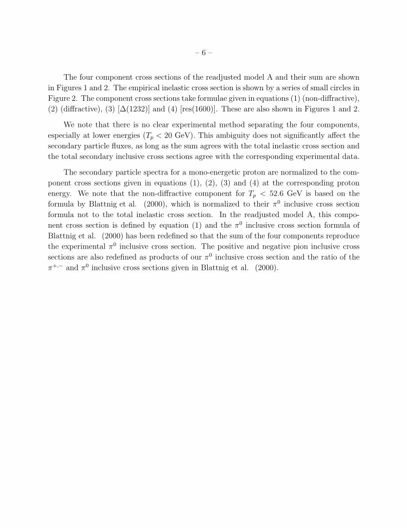
The four component cross sections of the readjusted model A and their sum are shown

in Figures 1 and 2. The empirical inelastic cross section is shown by a series of small circles in

Figure 2. The component cross sections take formulae given in equations (1) (non-diffractive),

(2) (diffractive), (3) [∆(1232)] and (4) [res(1600)]. These are also shown in Figures 1 and 2.

We note that there is no clear experimental method separating the four components,

especially at lower energies (Tp < 20 GeV). This ambiguity does not significantly affect the

secondary particle fluxes, as long as the sum agrees with the total inelastic cross section and

the total secondary inclusive cross sections agree with the corresponding experimental data.

The secondary particle spectra for a mono-energetic proton are normalized to the com-

ponent cross sections given in equations (1), (2), (3) and (4) at the corresponding proton

energy. We note that the non-diffractive component for Tp < 52.6 GeV is based on the

formula by Blattnig et al. (2000), which is normalized to their π0 inclusive cross section

formula not to the total inelastic cross section. In the readjusted model A, this compo-

nent cross section is defined by equation (1) and the π0 inclusive cross section formula of

Blattnig et al. (2000) has been redefined so that the sum of the four components reproduce

the experimental π0 inclusive cross section. The positive and negative pion inclusive cross

sections are also redefined as products of our π0 inclusive cross section and the ratio of the

π+,− and π0 inclusive cross sections given in Blattnig et al. (2000).

– 7 –

10.5

1

2

5

10

20

50

100

200

Pp [GeV/ ℄

� pp[mb℄

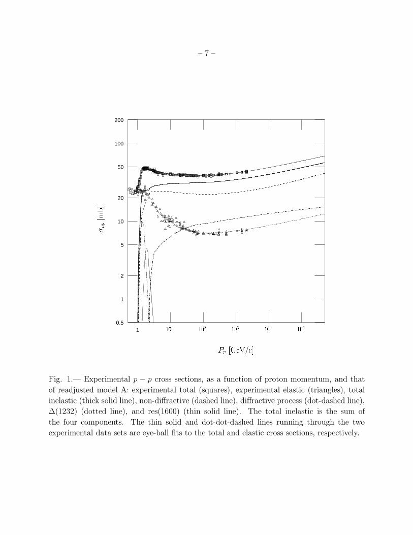
101 102 103 104 105Fig. 1.— Experimental p − p cross sections, as a function of proton momentum, and that

of readjusted model A: experimental total (squares), experimental elastic (triangles), total

inelastic (thick solid line), non-diffractive (dashed line), diffractive process (dot-dashed line),

∆(1232) (dotted line), and res(1600) (thin solid line). The total inelastic is the sum of

the four components. The thin solid and dot-dot-dashed lines running through the two

experimental data sets are eye-ball fits to the total and elastic cross sections, respectively.

– 8 –

1 2 5 100

10

20

30

40

Pp [GeV/ ℄

� pp;inel[mb℄

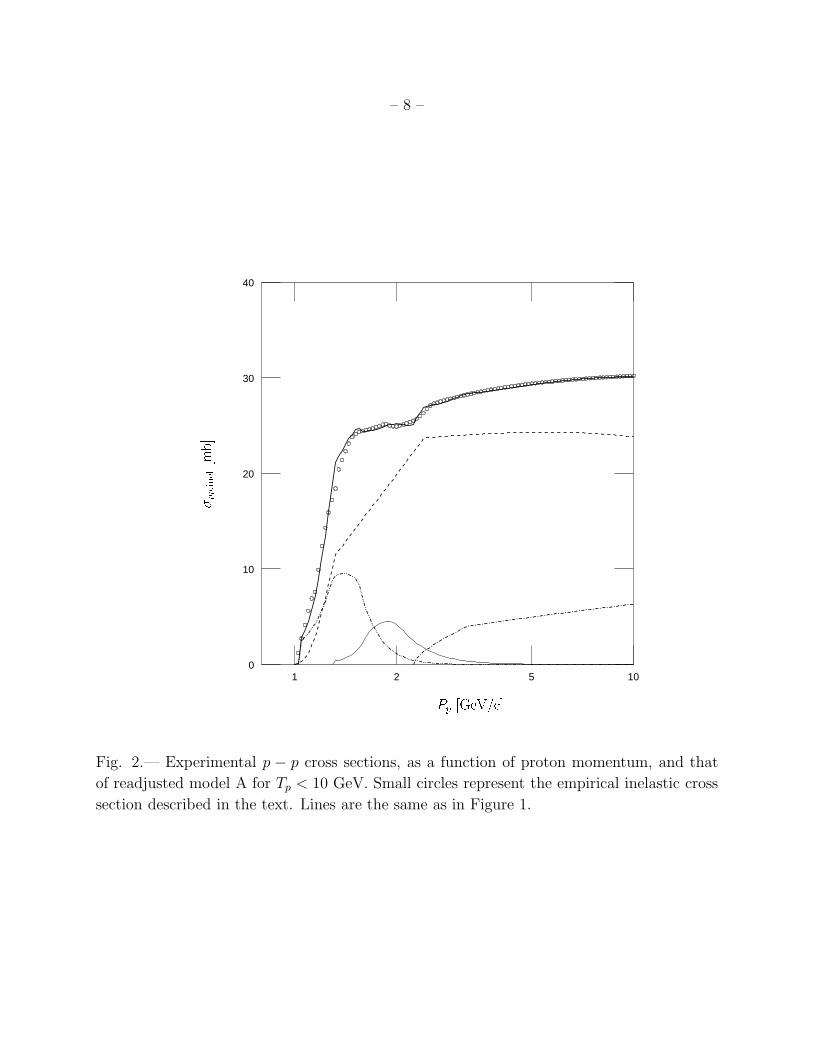
Fig. 2.— Experimental p − p cross sections, as a function of proton momentum, and that

of readjusted model A for Tp < 10 GeV. Small circles represent the empirical inelastic cross

section described in the text. Lines are the same as in Figure 1.

– 9 –

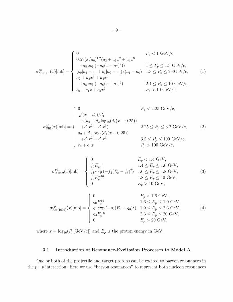
σppNonDiff(x)[mb] =

0 Pp < 1 GeV/c,

0.57(x/a0)1.2(a2 + a3x

2 + a4x3

+a5 exp(−a6(x + a7)2)) 1 ≤ Pp ≤ 1.3 GeV/c,

(b0|a1 − x| + b1|a0 − x|)/(a1 − a0) 1.3 ≤ Pp ≤ 2.4GeV/c,

a2 + a3x2 + a4x

3

+a5 exp(−a6(x + a7)2) 2.4 ≤ Pp ≤ 10 GeV/c,

c0 + c1x + c2x2 Pp > 10 GeV/c,

(1)

σppDiff(x)[mb] =

0 Pp < 2.25 GeV/c,√

(x − d0)/d1

×(d2 + d3 log10(d4(x − 0.25))

+d5x2 − d6x

3) 2.25 ≤ Pp ≤ 3.2 GeV/c,

d2 + d3 log10(d4(x − 0.25))

+d5x2 − d6x

3 3.2 ≤ Pp ≤ 100 GeV/c,

e0 + e1x Pp > 100 GeV/c,

(2)

σpp∆1232(x)[mb] =

0 Ep < 1.4 GeV,

f0E10p 1.4 ≤ Ep ≤ 1.6 GeV,

f1 exp (−f2(Ep − f3)2) 1.6 ≤ Ep ≤ 1.8 GeV,

f4E−10p 1.8 ≤ Ep ≤ 10 GeV,

0 Ep > 10 GeV,

(3)

σppRes(1600)(x)[mb] =

0 Ep < 1.6 GeV,

g0E14p 1.6 ≤ Ep ≤ 1.9 GeV,

g1 exp (−g2(Ep − g3)2) 1.9 ≤ Ep ≤ 2.3 GeV,

g4E−6p 2.3 ≤ Ep ≤ 20 GeV,

0 Ep > 20 GeV,

(4)

where x = log10(Pp[GeV/c]) and Ep is the proton energy in GeV.

3.1. Introduction of Resonance-Excitation Processes to Model A

One or both of the projectile and target protons can be excited to baryon resonances in

the p−p interaction. Here we use “baryon resonances” to represent both nucleon resonances

– 10 –

(iso-spin=1/2) and ∆ resonances (iso-spin=3/2). These excitations enhance the pion pro-

duction (and hence secondary particle production) near the inelastic threshold. The most

prominent resonance among them is ∆(1232), which has a mass of 1232 MeV/c2 and decays

predominantly (> 99%) to a nucleon and a pion (Hagiwara et al. 2002).

Stecker (1970) proposed a cosmic gamma-ray model in which neutral pions are produced

only through the ∆(1232) excitation for Tp ≤ 2.2 GeV. The resonance is assumed to move

only in the direction of the incident proton. At higher energies, another process, the fireball

process, sets in and produces pions with limited transverse momenta.

Dermer (1986a) compared predictions of models on π0 kinetic energy distribution in

the proton-proton center-of-mass (CM) system with experiments and noted that the model

by Stecker (1970) reproduces data better than the scaling model by Stephens & Badhwar

(1981) for Tp < 3 GeV. He proposed a cosmic gamma-ray production model that covers a

wider energy range by connecting the two models in the energy range Tp = 3 − 7 GeV.

Model A by Kamae et al. (2005) has been constructed primarily for the p − p inelastic

interaction Tp ≫ 1 GeV and has left room for improvement for Tp < 3 GeV. The diffrac-

tion dissociation component of model A has a resonance-excitation feature similar to that

implemented in Stecker (1971) for Tp > 3 GeV where either or both protons can be excited

to nucleon resonances (iso-spin=1/2 and mass around 1600 MeV/c2) along the direction of

the incident and/or target protons. What has not been implemented in model A is the en-

hancement by baryon resonances in the inclusive pion production cross sections below Tp < 3

GeV.

We note here that the the models by Stecker (1970) and by Dermer (1986a, see also

Dermer 1986b) used experimental data on the inclusive π0 yield (and that of charged pions)

to guide their modeling, but not the total inelastic cross section. Model A by Kamae et al.

(2005), on the other hand, has simulated all particles in each event (referred to as the “ex-

clusive” particle distribution) for all component cross sections. One exception is simulation

of the low-energy non-diffractive process (Tp < 52.6 GeV) by Blattnig et al. (2000). The

inclusive π0 (or gamma-ray) yield is obtained by collecting π0 (or gamma-rays) in simulated

exclusive events. When readjusting model A by adding the resonance-excitation feature

similar to that by Stecker (1970), overall coherence to model A has been kept. We adjusted

the ∆(1232) excitation cross section to reproduce the total inelastic cross section given in

Figure 2 and fixed the average pion multiplicities for + : 0 : − to those expected by the

one-pion-exchange hypothesis, 0.73 : 0.27 : 0.0. As higher-mass resonances begin to con-

tribute, the average pion multiplicity is expected to increase. To reproduce the experimental

π0 inclusive cross section and total inelastic cross section for Tp < 3 GeV, we introduced a

second resonance, res(1600). This resonance does not correspond to any specific resonance

– 11 –

but represents several baryon resonances at around 1600 MeV/c2: its pion multiplicities

(+ : 0 : −) are assumed to be 1.0:0.8:0.2. We note here that the resonance components favor

positive pions significantly over neutral pions while negative pions are strongly suppressed.

The distribution of pion kinetic energy in the p−p center-of-mass (CM) system (Tπ) has

been adjusted to reproduce the experimental ones given in Figs. 3-5 of Dermer (1986a). For

the ∆(1232) excitation, the probability increases proportionally to Tπ up to its maximum, set

at Tπ = 0.28×abs(Tp−0.4)0.45. Here Tπ and Tp are measured in GeV/c. The distribution goes

to zero beyond this maximum value. For res(1600), the probability distribution increases

proportionally to Tπ to reach its peak at Tπ = 0.16 × abs(Tp − 0.4)0.45. It decreases linearly

until reaching zero at twice the peak of Tπ.

Pion momentum is directed isotropically in the p−p CM system for res(1600) as well as

for ∆(1232). No angular correlation has been assumed between the two pions from res(1600):

this is justified for the astronomical environment where chance of detecting two gamma rays

from a same interaction is null. Decay kinematics including the polarization effect has been

implemented to the charged pion decay. This treatment allows the resonances to recoil

transversely to the direction of the incident proton while the recoil was constrained along

the incident proton direction in Stecker (1970).

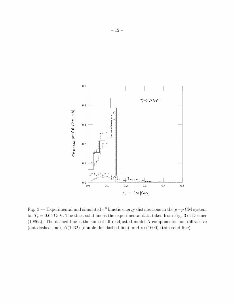
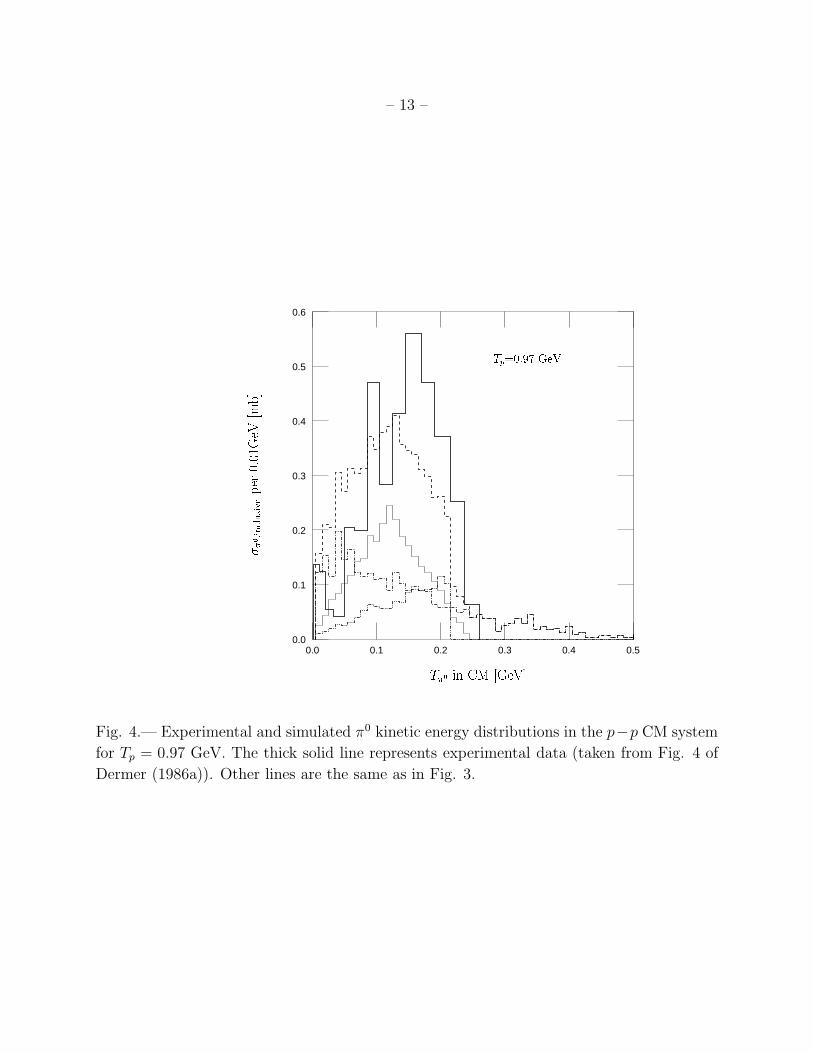
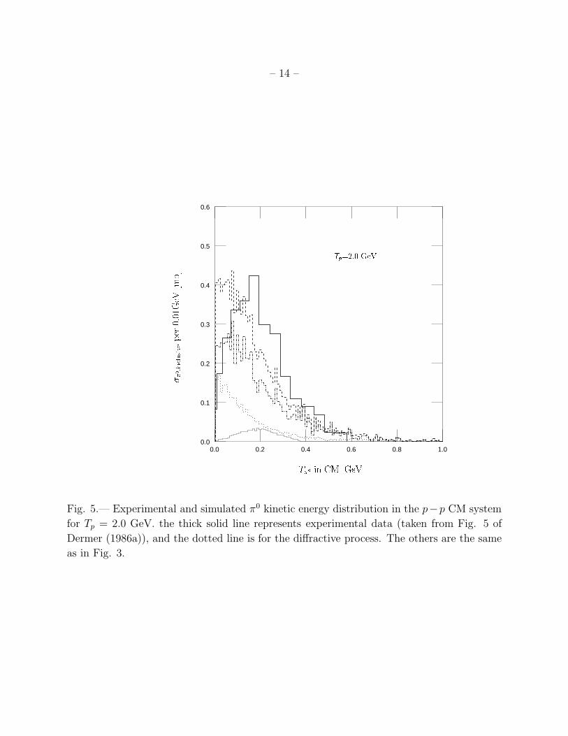
To validate the resonance components of the readjusted model A, we have compared the

model π0 spectrum in the p−p CM system at Tp = 0.65, 0.97, and 2.0 GeV with experimental

data in Figures 3, 4, 5. Shown in these figures are contributions of the ∆(1232), res(1600),

non-diffractive, and diffractive processes. Our model reproduces well the shape of pion

kinetic energy distribution at Tp = 0.65 GeV but begins to concentrate more towards zero

kinetic energy than experimental data at Tp = 0.97 and 2.0 GeV. Fidelity to the experimental

data is much improved when compared with the model by Stephens & Badhwar (1981) but

somewhat worse than the one by Stecker (1970) given in Figures 2-6 of Dermer (1986a). The

difference among the models becomes less noticeable for pion decay products, gamma-rays,

electrons, positrons, and neutrinos.

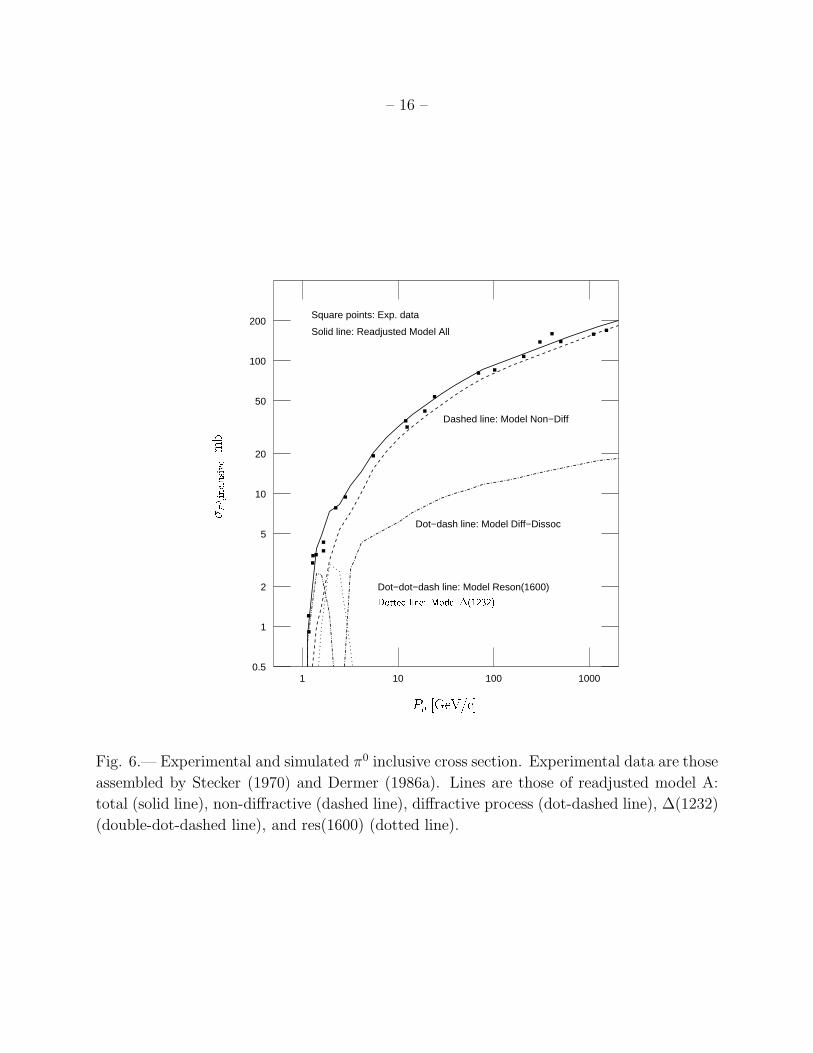
Our inclusive π0 cross section, sum of all four components, is compared with experimen-

tal data assembled by Stecker (1970) and Dermer (1986a) in Fig. 6. The readjusted model

A reproduces experimental data quite well for a wide range of incident proton energy.

– 12 –

0.0 0.1 0.2 0.3 0.4 0.50.0

0.1

0.2

0.3

0.4

0.5

Tp=0.65 GeV

T�0 in CM [GeV℄

� �0 ;in lusiveper0.01GeV[mb℄

Fig. 3.— Experimental and simulated π0 kinetic energy distributions in the p−p CM system

for Tp = 0.65 GeV. The thick solid line is the experimental data taken from Fig. 3 of Dermer

(1986a). The dashed line is the sum of all readjusted model A components: non-diffractive

(dot-dashed line), ∆(1232) (double-dot-dashed line), and res(1600) (thin solid line).

– 13 –

0.0 0.1 0.2 0.3 0.4 0.50.0

0.1

0.2

0.3

0.4

0.5

0.6 Tp=0.97 GeV

T�0 in CM [GeV℄� �0 ;in lusiveper0.01GeV[mb℄

Fig. 4.— Experimental and simulated π0 kinetic energy distributions in the p−p CM system

for Tp = 0.97 GeV. The thick solid line represents experimental data (taken from Fig. 4 of

Dermer (1986a)). Other lines are the same as in Fig. 3.

– 14 –

0.0 0.2 0.4 0.6 0.8 1.00.0

0.1

0.2

0.3

0.4

0.5

0.6

Tp=2.0 GeV

T�0 in CM [GeV℄

� �0 ;in lusiveper0.01GeV[mb℄

Fig. 5.— Experimental and simulated π0 kinetic energy distribution in the p−p CM system

for Tp = 2.0 GeV. the thick solid line represents experimental data (taken from Fig. 5 of

Dermer (1986a)), and the dotted line is for the diffractive process. The others are the same

as in Fig. 3.

– 15 –

4. Inclusive Spectra of Simulated Events for Mono-Energetic Proton Beam

The first step of parameterization is to generate simulated events for mono-energetic

protons. To simplify this step, events have been generated for discrete proton energies at a

geometrical series of Tp = 1000.0 × 2(N−22)/2 GeV where N = 0 − 40. Each proton kinetic

energy (Tp) represents a bin covering between 2−0.25Tp and 20.25Tp. The sampling density

has been increased for Tp < 1 GeV by adding points at Tp = 0.58 GeV and 0.82 GeV.

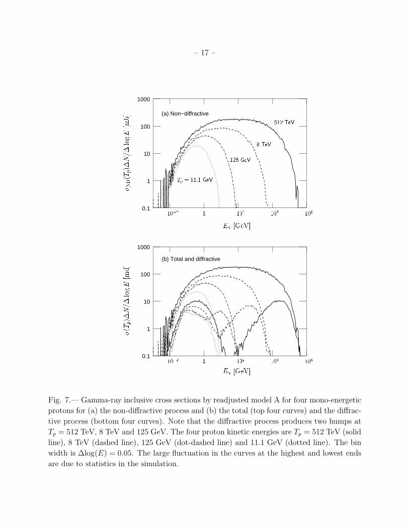
Secondary particle spectra are histogrammed from these simulated events in energy bins

of width ∆E/E = 5 %. Figures 7a and 7b show thus-obtained inclusive gamma-ray cross

sections for the non-diffractive and diffractive processes, for Tp = 512 TeV, 8 TeV, 125 GeV

and 11.1 GeV respectively. Those for e± are given for Tp = 8 TeV and 512 TeV in Figures

8a and 8b.

– 16 –

Solid line: Readjusted Model All

Square points: Exp. data

Dashed line: Model Non−Diff

Dot−dash line: Model Diff−Dissoc

Dot−dot−dash line: Model Reson(1600)

1 10 100 10000.5

1

2

5

10

20

50

100

200

Dotted line: Model �(1232)Pp [GeV/ ℄

� �0 ;in lusive[mb℄

Fig. 6.— Experimental and simulated π0 inclusive cross section. Experimental data are those

assembled by Stecker (1970) and Dermer (1986a). Lines are those of readjusted model A:

total (solid line), non-diffractive (dashed line), diffractive process (dot-dashed line), ∆(1232)

(double-dot-dashed line), and res(1600) (dotted line).

– 17 –

1

(a) Non−diffractive

(b) Total and diffractive

0.1

1

10

100

1000

10.1

1

10

100

1000

E [GeV℄

E [GeV℄

�(T p)�N=�logE[md℄

� ND(T p)�N=�logE[mb℄

10�2 102 104125 GeV 8 TeV 512 TeV

Tp = 11:1 GeV106

10�2 102 104 106Fig. 7.— Gamma-ray inclusive cross sections by readjusted model A for four mono-energetic

protons for (a) the non-diffractive process and (b) the total (top four curves) and the diffrac-

tive process (bottom four curves). Note that the diffractive process produces two humps at

Tp = 512 TeV, 8 TeV and 125 GeV. The four proton kinetic energies are Tp = 512 TeV (solid

line), 8 TeV (dashed line), 125 GeV (dot-dashed line) and 11.1 GeV (dotted line). The bin

width is ∆log(E) = 0.05. The large fluctuation in the curves at the highest and lowest ends

are due to statistics in the simulation.

– 18 –

1

(a) Non−diffractive

(b) Diffractive

0.1

1

10

100

1000

10.1

1

10

100

1000

Ee� [GeV℄

Ee� [GeV℄10�2 102 104 106

�(T p)�N=�logE[mb℄� ND(T p)�N=�logE[mb℄

10�2 102Tp = 8 TeV 512 TeV

Tp = 8 TeV 512 TeV

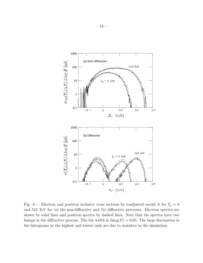
104 106Fig. 8.— Electron and positron inclusive cross sections by readjusted model A for Tp = 8

and 512 TeV for (a) the non-diffractive and (b) diffractive processes. Electron spectra are

shown by solid lines and positron spectra by dashed lines. Note that the spectra have two

humps in the diffractive process. The bin width is ∆log(E) = 0.05. The large fluctuation in

the histograms at the highest and lowest ends are due to statistics in the simulation.

– 19 –

We then define, after several iterations of fitting, functional formulae that reproduce

the secondary particle spectra for mono-energetic protons, for the non-diffractive, diffractive,

and resonance-excitation processes separately. For the non-diffractive process, the differential

inclusive cross section (∆σND) to produce a secondary particle in a bin of width ∆Esec/Esec =

100 % centered at Esec is given as

∆σND(Esec)

∆ log(Esec)= FND(x)FND,kl(x), (5)

where Esec[GeV] is the energy of the secondary particle and x = log10(Esec[GeV]).

FND(x) is the formula representing the non-diffractive cross section, given in equation (6)

below, and FND,kl(x) is the formula to approximately enforce the energy-momentum conser-

vation limits:

FND(x) = a0 exp(−a1(x − a3 + a2(x − a3)2)2) +

a4 exp(−a5(x − a8 + a6(x − a8)2 + a7(x − a8)

3)2), (6)

FND,kl(x) =1

(exp (WND,l(Lmin − x)) + 1)

1

(exp (WND,h(x − Lmax)) + 1), (7)

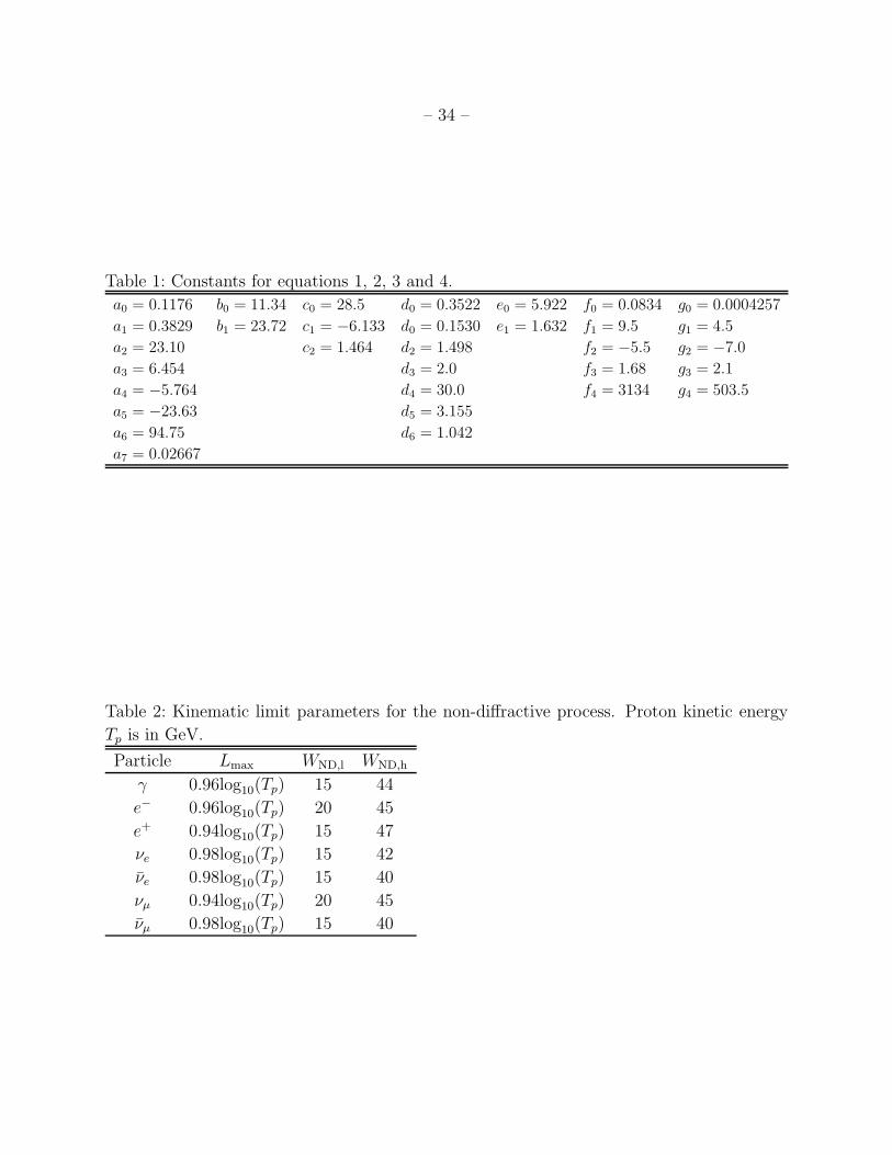
where Lmin and Lmax are the lower and upper kinematic limits imposed and WND,l and

WND,h are the widths of the kinematic cut-offs; Lmin = −2.6 for all secondary particles, and

the other parameters are listed in Table 2.

For the diffractive process we use a similar function

∆σdiff(Esec)

∆ log(Esec)= Fdiff(x)Fkl(x) (8)

where Esec[GeV] is the energy of the secondary particle and x = log10(Esec[GeV]);

Fdiff(x) represents the diffractive cross section, given in equation (9) below, and Fkl(x) en-

forces the energy-momentum conservation:

FDiff(x) = b0 exp(−b1((x − b2)/(1 + b3(x − b2)))2) +

b4 exp(−b5((x − b6)/(1 + b7(x − b6)))2), (9)

– 20 –

Fkl(x) =1

exp (Wdiff(x − Lmax)) + 1, (10)

with Wdiff = 75 and Lmax = log10(Tp[GeV ]).

For the resonance-excitation processes [∆(1232) and res(1600)] we use the function,

∆σres(Esec)

∆ log(Esec)= Fres(x)Fkl(x), (11)

where Esec[GeV] is the energy of the secondary particle and x = log10(Esec[GeV]), Fres(x)

represents the cross section, given in equation (12) below, and Fkl(x), which is the same as

for the diffraction process, enforces the energy-momentum conservation:

Fres(x) = c0 exp (−c1((x − c2)/(1 + c3(x − c2) + c4(x − c2)2))2). (12)

To ensure that the parameterized model reproduces the experimental π0 multiplicity

after the readjustment in the resonance-excitation region of Tp, we have renormalized the

non-diffractive contribution by multiplying it with a renormalization factor, r(Tp), given

below, to the final spectrum. Note that this readjustment does not affected the diffractive

process.

r(Tp) ≃ 1.01 for Tp > 1.95GeV, (13)

r(y = log10(Tp)) = 3.05 exp (−107((y + 3.25)/(1 + 8.08(y + 3.25)))2) for Tp ≤ 1.95GeV.

(14)

For all other secondary particles, r(y = log10(Tp)) is found in Tables 4-9.

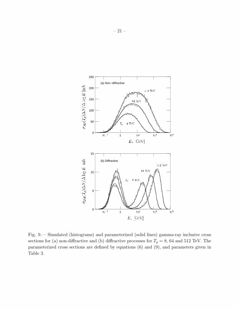
The simulated gamma-ray inclusive cross sections are superimposed with the parame-

terized ones in Figures 9a and 9b for three mono-energetic protons, for the non-diffractive

and diffractive processes and for the resonance-excitation processes in Figure 10. The agree-

ment is generally good except near the higher and lower kinematical limits where we find a

difference of about 10-20%.

– 21 –

10

5

10

15

1

(a) Non−diffractive

(b) Diffractive

0

50

100

150

200

250

10�2 102 104 106

E [GeV℄

E [GeV℄� Di�(T p)�N=�logE[mb℄� ND(T p)�N=�logE[mb℄

10�2 102

512 TeV64 TeVTp = 8 TeV

512 TeV64 TeVTp = 8 TeV

104 106

Fig. 9.— Simulated (histograms) and parameterized (solid lines) gamma-ray inclusive cross

sections for (a) non-diffractive and (b) diffractive processes for Tp = 8, 64 and 512 TeV. The

parameterized cross sections are defined by equations (6) and (9), and parameters given in

Table 3.

– 22 –

1 100

1

2

3

E [GeV℄�(T p)�N=�logE[mb℄

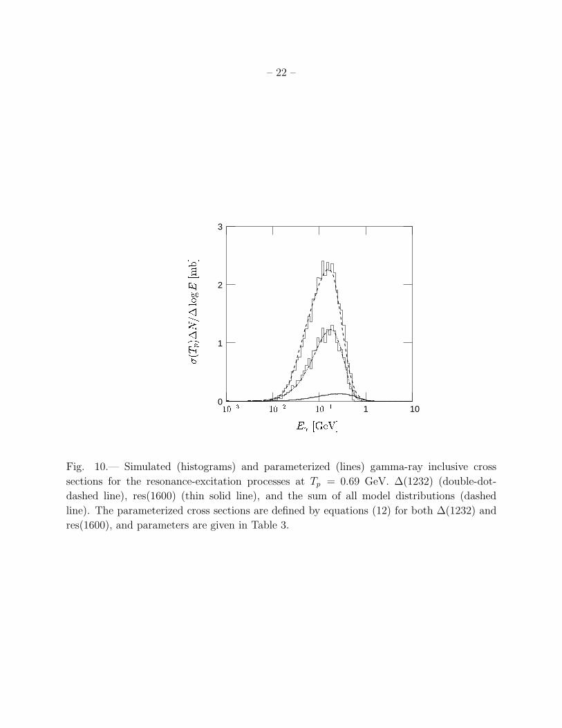
10�3 10�2 10�1Fig. 10.— Simulated (histograms) and parameterized (lines) gamma-ray inclusive cross

sections for the resonance-excitation processes at Tp = 0.69 GeV. ∆(1232) (double-dot-

dashed line), res(1600) (thin solid line), and the sum of all model distributions (dashed

line). The parameterized cross sections are defined by equations (12) for both ∆(1232) and

res(1600), and parameters are given in Table 3.

– 23 –

5. Representation of Parameters as Functions of Incident Proton Energy

The parameterization formulae for secondary particles for mono-energetic protons (equa-

tions [6], [9] and [12]) have nine, eight, and five parameters for each Tp for non-diffractive,

diffractive, and resonance-excitation processes respectively. These parameters depend on the

proton kinetic energy, Tp. The final step of the parameterization is to find simple functions

representing energy dependence of these parameters. Functions obtained by fitting often

give values different significantly from those found for mono-energetic protons near the kine-

matic limits and produce artifacts in the wide range spectral energy density, as described

previously. Some manual adjustments have been made to control possible artifacts.

5.1. Parameterized Gamma Ray Spectrum

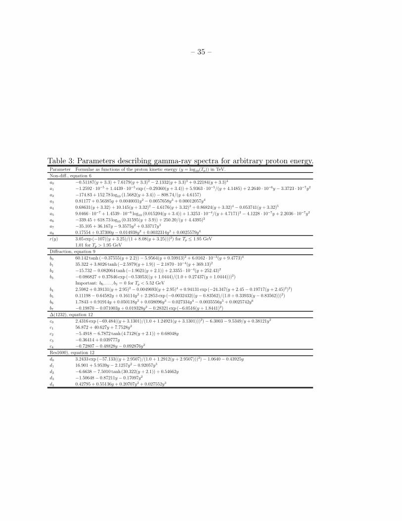
The final functional representation of inclusive cross sections for secondary gamma-rays

is given in equations (6), (9), and (12) with parameters defined as functions of Tp in TeV

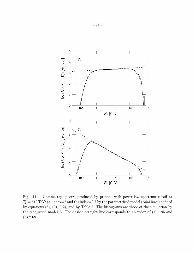
(not GeV) in Table 3. The total inclusive gamma-ray spectrum is the sum of the non-

diffractive, diffractive, and resonance-excitation contributions. The spectrum produced by

protons with a continuous spectrum can be calculated by summing over the total gamma-

ray spectra for mono-energetic protons with appropriate spectral weight. For example, the

spectra for power-law protons extending to Tp = 512 TeV with index=2 and index=2.7

have been calculated and compared with the corresponding histograms produced from the

simulated events in Figure 11. The parameterized model reproduces either spectrum within

10%: it predicts 10-20% more gamma-rays than simulation by the readjusted model A at

the higher kinematical limit.

– 24 –

1

(a)

(b)

0

1

2

3

4

5

10

2

4

6

8

E [GeV℄

E [GeV℄log(E�Flux(E))[relative℄

log(E�Flux(E))[relative℄

10�2 102 104 106

10�2 102 104 106Fig. 11.— Gamma-ray spectra produced by protons with power-law spectrum cutoff at

Tp = 512 TeV: (a) index=2 and (b) index=2.7 by the parametrized model (solid lines) defined

by equations (6), (9), (12), and by Table 3. The histograms are those of the simulation by

the readjusted model A. The dashed straight line corresponds to an index of (a) 1.95 and

(b) 2.68.

– 25 –

5.2. Parameterized e± and Neutrino Spectra

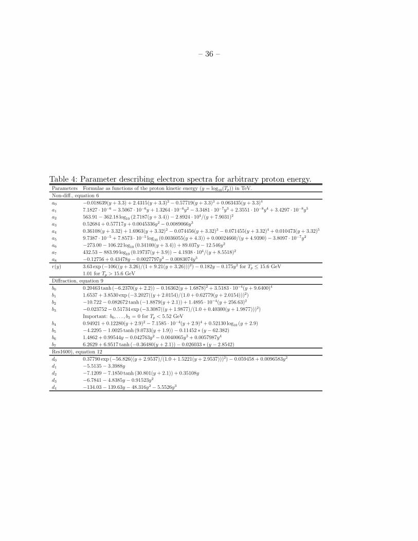
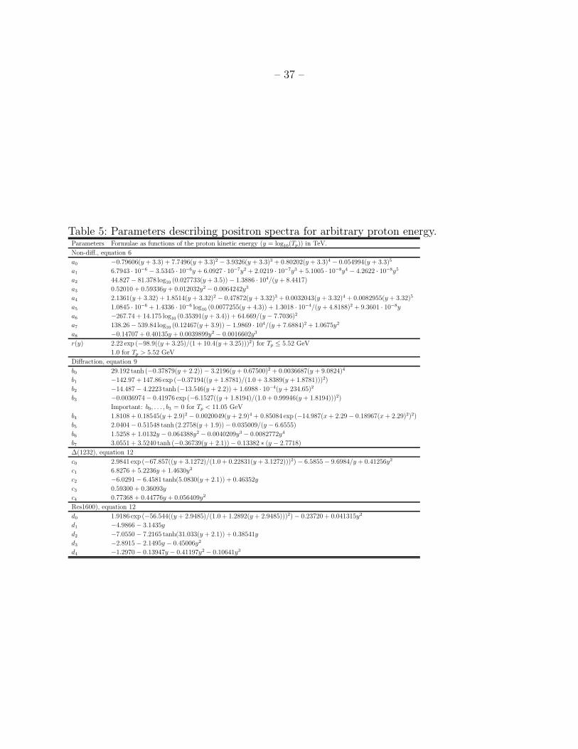
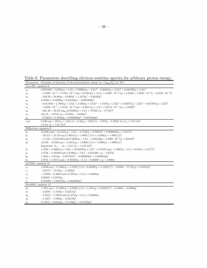
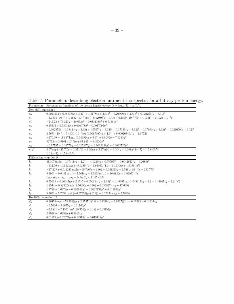
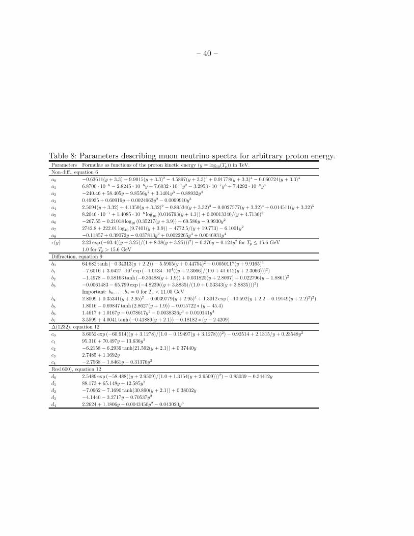
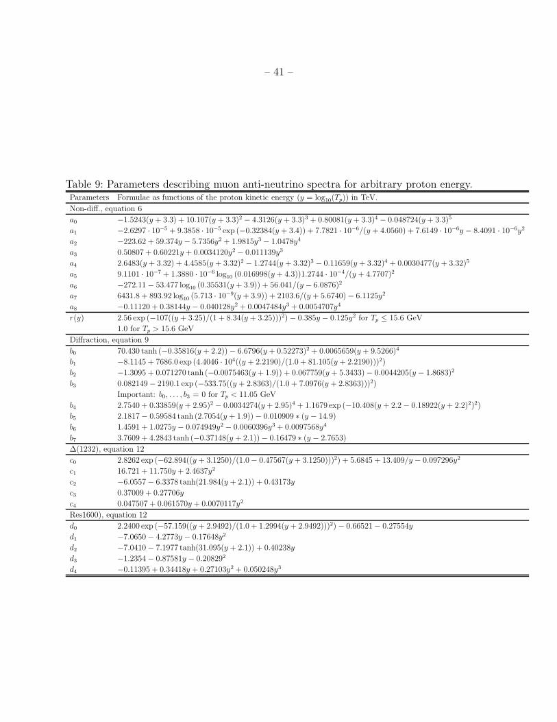
The parameterization has been extended to other secondary particles, e−, e+, νe, νe,

νµ, and νµ, in the same way as for gamma-rays. Their functional formulae are represented

by equations (6), (9), and (12) with the parameters defined in Tables 4, 5, 6, 7, 8, and 9,

respectively. We note that no π− is produced in ∆(1232) decay in readjusted model A and,

hence, no e− and νe either.

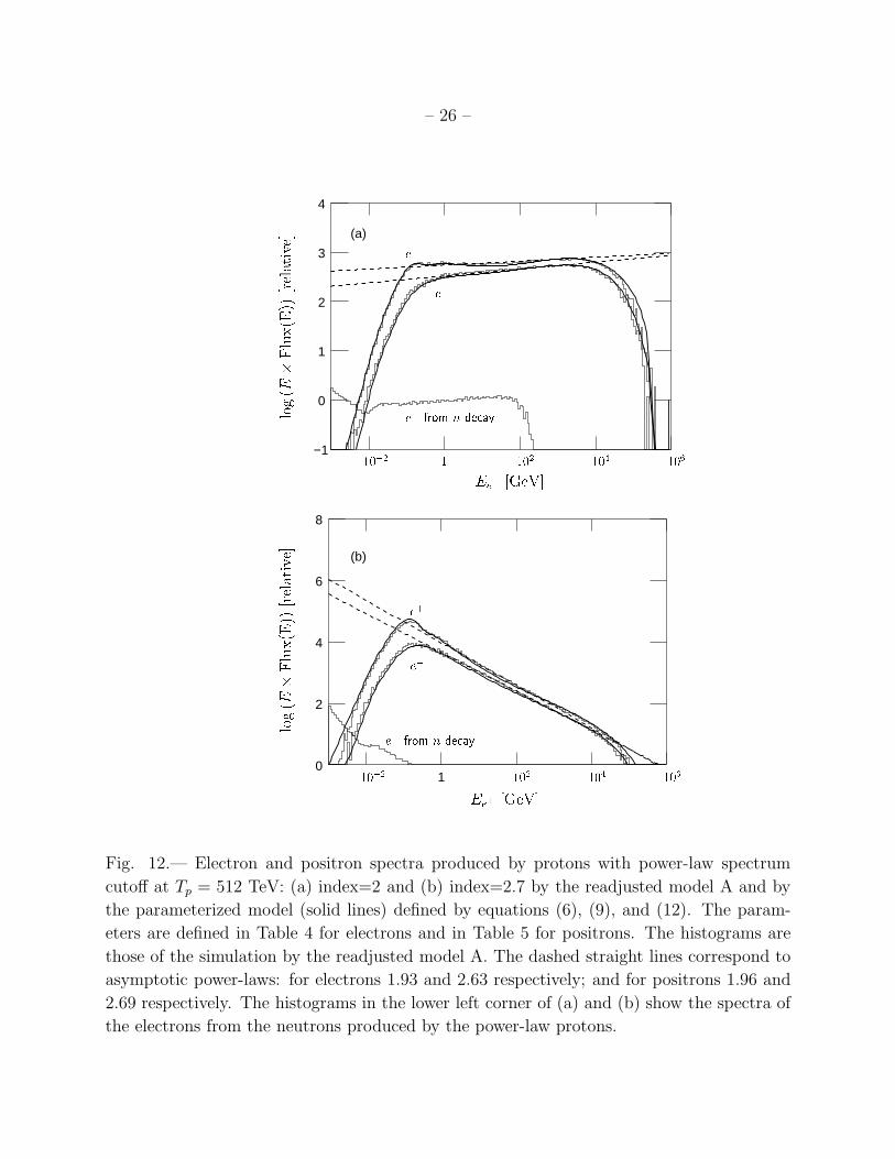
We note that the secondary electron and positron spectra from charged pion and muon

decays have been calculated including the polarization effect of the weak interaction theory.

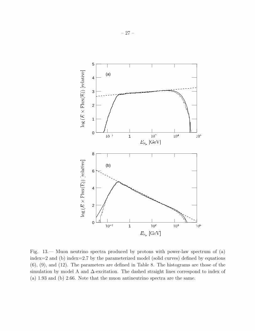
The spectra produced by power-law protons of index=2.0 and 2.7 (Tp < 512 TeV) have been

computed based on these parameterized models in Figure 12 for e± and Figure 13 for νµ.

We note in Figure 12 that more e+ are produced than e− throughout their spectra. This

is largely due to the charge conservation and enhanced by the fact that we have neglected

α-particles and neutron decays. The number of electrons produced in the p − p interaction

will match that of positrons if we include electrons coming out of neutron decays.

For given Tp, electrons from neutron decays have low energy (mostly with E < 10 MeV)

as shown by the lower histograms in Figure 12. They do not contribute to the high energy

gamma-ray spectrum.

– 26 –

−1

0

1

2

3

4

(b)

(a)

10

2

4

6

8

Ee� [GeV℄

Ee� [GeV℄

log(E�Flux(E))[relative℄

log(E�Flux(E))[relative℄

10�2 1 102 104 106

10�2e� from n de ay

e� from n de ay

e�e+

e+ e�

102 104 106Fig. 12.— Electron and positron spectra produced by protons with power-law spectrum

cutoff at Tp = 512 TeV: (a) index=2 and (b) index=2.7 by the readjusted model A and by

the parameterized model (solid lines) defined by equations (6), (9), and (12). The param-

eters are defined in Table 4 for electrons and in Table 5 for positrons. The histograms are

those of the simulation by the readjusted model A. The dashed straight lines correspond to

asymptotic power-laws: for electrons 1.93 and 2.63 respectively; and for positrons 1.96 and

2.69 respectively. The histograms in the lower left corner of (a) and (b) show the spectra of

the electrons from the neutrons produced by the power-law protons.

– 27 –

1

(a)

(b)

0

1

2

3

4

5

10

2

4

6

8

E�� [GeV℄

E�� [GeV℄log(E�Flux(E))[relative℄log(E�Flux(E))[relative℄

10�2 102 104 106

10�2 102 104 106Fig. 13.— Muon neutrino spectra produced by protons with power-law spectrum of (a)

index=2 and (b) index=2.7 by the parameterized model (solid curves) defined by equations

(6), (9), and (12). The parameters are defined in Table 8. The histograms are those of the

simulation by model A and ∆-excitation. The dashed straight lines correspond to index of

(a) 1.93 and (b) 2.66. Note that the muon antineutrino spectra are the same.

– 28 –

0.05 0.1 0.2 0.5 1 2 5 100.05

0.1

0.2

E [GeV℄E2 �Flux[relative℄

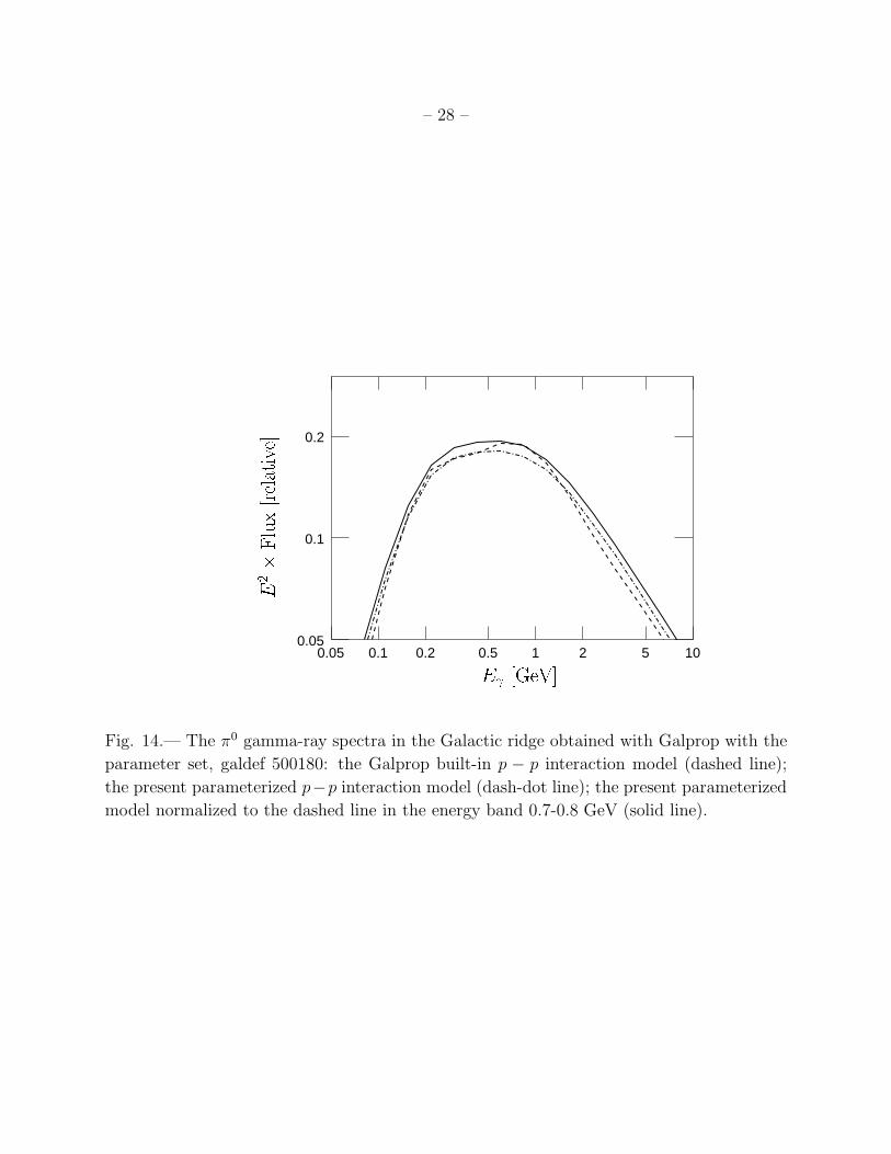
Fig. 14.— The π0 gamma-ray spectra in the Galactic ridge obtained with Galprop with the

parameter set, galdef 500180: the Galprop built-in p − p interaction model (dashed line);

the present parameterized p−p interaction model (dash-dot line); the present parameterized

model normalized to the dashed line in the energy band 0.7-0.8 GeV (solid line).

– 29 –

6. Application to Galactic Diffuse Gamma-Ray Emission

We have replaced the π0 production subroutine of Galprop (Strong & Moskalenko 1997,

2001) with the present parameterized model and compared the Galactic diffuse gamma-ray

spectra of π0 origin with that by the built-in subroutine. A common parameter set, galdef

500180 described in Strong et al. (2004), has been used in the two calculations.

As shown in Figure 14, the present parameterized model gives a flatter and smoother

spectral energy distribution between Eγ = 0.3 − 2 GeV, smaller gamma-ray yield between

0.5 − 1.3 GeV, and a higher power-law index between 1 − 5 GeV than the Galprop built-in

model. In Kamae et al. (2005), gamma-ray spectrum of the Galprop built-in model was

compared with that of model A, after being normalized in the energy range E < 300 MeV.

This normalization enhanced gamma-ray yield in the GeV range relative to sub-GeV range.

The Galprop built-in p−p interaction model has been tuned to reproduce accelerator experi-

ments better than model A of Kamae et al. (2005) near the threshold. We have included the

resonance contributions in the present model to improve this shortcoming near the thresh-

old. Hence we have change the normalization point to the peak region in E2dflux/dE,

Eγ = 0.7 − 0.8 GeV, where gamma-rays from π0 decays are expected to dominate (see Fig-

ure 14, dashed curve). The present model thus normalized gives ∼ 20% higher gamma-ray

yield than Galprop at 2 GeV: this is substantially lower than the difference (about 50%)

shown in Figure 7 of Kamae et al. (2005). The gamma-ray power-law index of the present

model is harder by about 0.05 than that by the Galprop built-in model, just as the model

A of Kamae et al. (2005) predicts.

7. Conclusion and Future Prospects

We have presented the inclusive cross sections of stable secondary particles (γ, e±, νe,

νe, νµ, and νµ) produced by the p−p interaction in parameterized formulae. They facilitates

computation of secondary particle spectra for arbitrary proton spectra as shown for Galactic

diffuse gamma-ray spectrum (Figure 14). Various effects that these secondary particles may

have in astronomical environments can also be calculated at a higher precision. The formulae

incorporate all important known features of the p− p interaction up to about Tp = 500 TeV

and hence will also be useful in calculating background when searching for new phenomena.

The parameterized model predicts all secondary particle spectra to have harder power-

law indices than that of the incident proton and their inclusive cross sections to be larger

than those expected from the old p − p interaction models. When used to replace the p − p

subroutine in Galprop (Strong & Moskalenko 1997, 2001), the model gives a flatter spectral

– 30 –

energy density distribution between 0.3−5 GeV. The absolute gamma-ray yield predicted by

the model is smaller than that by the Galprop model for Eγ < 1.5 GeV but higher for Eγ >

1.5 GeV. If normalized near the peak in E2dflux/dE (Eγ = 0.7−0.8 GeV), the parameterized

model gives ∼ 20% higher gamma-ray yield at 2 GeV than the model of Galprop: our model

with this normalization can account for ∼ 20%, not ∼ 50% as was claimed in Kamae et al.

(2005), of the discrepancy between the diffuse Galactic Ridge gamma-ray spectrum observed

by EGRET and model predictions for the proton spectrum near the solar system (the power-

law index ∼ 2.7) (Hunter et al. 1997). We note the discrepancy will be reduced by inclusion

of the inverse Compton component (see, for example, a model by Strong et al. (2004)).

The present model also predicts more e+ than e− at energies higher wherever those

produced by p − p interaction become comparable in flux to primary e− and e+. The

formulae and parameters given in the appendices are available as supplementary on-line

material both in C language format and as C subroutine. We are currently parametrizing

the angular distribution of gamma-rays relative to the incident proton direction. The results

will be published elsewhere.

8. Acknowledgments

The authors would like to acknowledge valuable discussions with and comments received

from M. Asai, E. Bloom, P. Carlson, J. Chiang, J. Cohen-Tanugi, S. Digel, E. do Couto e

Silva, I. Grenier, G. Madejski, I. Moskalenko, P. Nolan, O. Reimer, D. Smith, F. Stecker,

A. Strong, H. Tajima, and L. Wai. They wish to thank the anonimous referee for valuable

comments and suggestions.

REFERENCES

Aharonian, F. A., 2004, “Very High Energy Cosmic Gamma Radiation: A Crucial Window

on the Extreme Universe” (World Scientific Publishing)

Aharonian, F. A., 2005, Science, 307, 1938: available as astro-ph/0504380

Aharonian, F. A., et al., 2004b, Nature, 432, 75: available as astro-ph/0411533

Aharonian, F. A., et al., 2004c, A&A, 425, L13: available as astro-ph/0408145

Aharonian, F. A., Volk , Horns, D. 2004, Proc. Int. Symp. on High Energy Gamma-Ray

Astronomy (World Scientific)

– 31 –

Berezhko, E. G. & Volk, H. J., 2000, ApJ, 540, 923

Blattnig, S. R., et al. 2000, Phys. Rev., D62, 094030

Bloemen, J.B.G.M., et al. 1984, A&A, 135, 12

Bloemen, J.B.G.M. 1985, A&A, 145, 391

Bottcher, M. and Reimer, A. 2004 ApJ 609, 576

Crawford, J. F. et al. 1980 Phys. Rev. C22, 1184

Dermer, C. D. 1986a, A&A, 157, 223

Dermer, C. D. 1986b, ApJ, 307, 47

DuVernois, M.A., et al. 2001, ApJ 559, 296

Enomoto, R., et al., 2002, Nature, 416, 823: available as astro-ph/0204422

Field, R.D. 2002, Matrix Element and Monte Carlo Tuning Workshop,

http://cepa.fnal.gov/CPD/MCTuning, http://www.phys.ufl.edu/~rfield/cdf

Hagiwara, K., et al. 2002, Phys. Rev., D66, 010001.

Halzen, F., in Aharonian, F. A., Volk, H. J., and Horns, D. (eds.) Proc. Second Int. Sympo-

sium on High Energy Gamma-Ray Astronomy (July 2004, Heidelberg) p.3

Hayakawa, S. 1969, “Cosmic Ray Physics” (John-Wiley)

Hunter, S.D., et al. 1997, ApJ, 481, 205

Iyudin, A. F., et al. 2005, A&A 429, 225

Kamae, T., Abe., T, & Koi, T., 2005, ApJ 620, 244

Katagiri, H., et al., 2005, ApJ, 619, L163: available as astro-ph/0412623

Koyama, K., et al. 1997, PASJ 49, L7

Martensson, J., et al. 2000 Phys. Rev. C62, 014610

Mayer-Hasselwander, H.A., et al. 1982, A&A, 105, 164

Mori, M. 1997, ApJ, 478, 225

Mucke, A., and Protheroe, R. J. 2001, Astroparticle Physics 15, 121

– 32 –

Mucke, A., et al. 2003, Astroparticle Physics 18, 593

Muller, D. 2001, Adv. Space Res. 27, 659

Murthy, P.V.R. and Wolfendale, A. W. 1986, “Gamma-ray Astronomy” (Cambridge Univer-

sity Press)

Ong, R. A., 1998, Physics Reports, 305, 93

PAMELA Collaboration, see http://wizard.roma2.infn.it/pamela

Schonfelder, V. (ed) 2001, “The Universe in Gamma Rays” (Springer-Verlag)

Schlickeiser, R. 2002, “Cosmic Ray Astrophysics”, Springer Verlag

Sjostrand, T., Lonnblad, L., and Mrenna, S. 2001, “Pythia 6.2: Physics and Manual”,

hep-ph/0108264

Sjostrand, T., and Skands, P. Z. 2004, hep-ph/0402078

Slane, P., et al. 1999, ApJ 525, 357

Stanev, T., 2004, “High Energy Cosmic Rays” (Springer Verlag)

Stecker, F. 1970, Astrophys. & Space Science, 377

Stecker, F. 1971, “Cosmic Gamma Rays” NASA SP-249 (NASA Scientific and Technical

Information Office)

Stecker, F. 1973, ApJ, 185, 499

Stecker, F. 1990, in Shapiro, M.M., and Wefel, J.P. (eds.), “Cosmic Gamma Rays, Neutrinos

and Related Astrophysics”, p.89

Stephens, S.A., and Badhwar, G.D. 1981, Astrophys. Space Sci, 76, 213

Stephens, S.A. 2001, Adv. Space Res. 27, 687

Strong, A.W., et al. 1978, MNRAS, 182, 751

Strong, A.W., et al. 1982, A&A, 115, 404

Strong, A.W., and Moskalenko, I.V. 1997, Proc. Fourth Compton Symp., (eds) Dermer, C.

D., Strickman, M. S., and Kurfess, J. D., p.1162; astro-ph/9709211

– 33 –

Strong, A. W., and Moskalenko, I. V. 2001, Proc. of 27th ICRC 2001 (Hamburg), p.1942

and astro-ph/0106504

Strong, A. W., Moskalenko, I. V., and Reimer, O. 2000, ApJ, 537, 763; Errortum: 2000,

ibid, 541, 1109

Strong, A. W., Moskalenko, I. V., and Reimer, O. 2004, ApJ, 613, 962

Tsunemi, H., et al. 2000, PASJ 52, 887

Uchiyama, Y, Aharonian, F. A., and Takahashi, T. 2003, A&A 400, 567

Weekes, T. C., 2003, Proc. 28th Int. Cosmic Ray Conf. (Aug. 2003, Tsukuba): available as

astro-ph/0312179

This preprint was prepared with the AAS LATEX macros v5.2.

– 34 –

Table 1: Constants for equations 1, 2, 3 and 4.

a0 = 0.1176 b0 = 11.34 c0 = 28.5 d0 = 0.3522 e0 = 5.922 f0 = 0.0834 g0 = 0.0004257

a1 = 0.3829 b1 = 23.72 c1 = −6.133 d0 = 0.1530 e1 = 1.632 f1 = 9.5 g1 = 4.5

a2 = 23.10 c2 = 1.464 d2 = 1.498 f2 = −5.5 g2 = −7.0

a3 = 6.454 d3 = 2.0 f3 = 1.68 g3 = 2.1

a4 = −5.764 d4 = 30.0 f4 = 3134 g4 = 503.5

a5 = −23.63 d5 = 3.155

a6 = 94.75 d6 = 1.042

a7 = 0.02667

Table 2: Kinematic limit parameters for the non-diffractive process. Proton kinetic energy

Tp is in GeV.

Particle Lmax WND,l WND,h

γ 0.96log10(Tp) 15 44

e− 0.96log10(Tp) 20 45

e+ 0.94log10(Tp) 15 47

νe 0.98log10(Tp) 15 42

νe 0.98log10(Tp) 15 40

νµ 0.94log10(Tp) 20 45

νµ 0.98log10(Tp) 15 40

– 35 –

Table 3: Parameters describing gamma-ray spectra for arbitrary proton energy.Parameter Formulae as functions of the proton kinetic energy (y = log10(Tp)) in TeV.

Non-diff., equation 6

a0 −0.51187(y + 3.3) + 7.6179(y + 3.3)2 − 2.1332(y + 3.3)3 + 0.22184(y + 3.3)4

a1 −1.2592 · 10−5 + 1.4439 · 10−5 exp (−0.29360(y + 3.4)) + 5.9363 · 10−5/(y + 4.1485) + 2.2640 · 10−6y − 3.3723 · 10−7y2

a2 −174.83 + 152.78 log10 (1.5682(y + 3.4)) − 808.74/(y + 4.6157)

a3 0.81177 + 0.56385y + 0.0040031y2 − 0.0057658y3 + 0.00012057y4

a4 0.68631(y + 3.32) + 10.145(y + 3.32)2 − 4.6176(y + 3.32)3 + 0.86824(y + 3.32)4 − 0.053741(y + 3.32)5

a5 9.0466 · 10−7 + 1.4539 · 10−6 log10 (0.015204(y + 3.4)) + 1.3253 · 10−4/(y + 4.7171)2 − 4.1228 · 10−7y + 2.2036 · 10−7y2

a6 −339.45 + 618.73 log10 (0.31595(y + 3.9)) + 250.20/(y + 4.4395)2

a7 −35.105 + 36.167y − 9.3575y2 + 0.33717y3

a8 0.17554 + 0.37300y − 0.014938y2 + 0.0032314y3 + 0.0025579y4

r(y) 3.05 exp (−107((y + 3.25)/(1 + 8.08(y + 3.25)))2) for Tp ≤ 1.95 GeV

1.01 for Tp > 1.95 GeV

Diffraction, equation 9

b0 60.142 tanh (−0.37555(y + 2.2)) − 5.9564(y + 0.59913)2 + 6.0162 · 10−3(y + 9.4773)4

b1 35.322 + 3.8026 tanh (−2.5979(y + 1.9)) − 2.1870 · 10−4(y + 369.13)2

b2 −15.732 − 0.082064 tanh (−1.9621(y + 2.1)) + 2.3355 · 10−4(y + 252.43)2

b3 −0.086827 + 0.37646 exp (−0.53053((y + 1.0444)/(1.0 + 0.27437(y + 1.0444)))2)

Important: b0, . . . , b3 = 0 for Tp < 5.52 GeV

b4 2.5982 + 0.39131(y + 2.95)2 − 0.0049693(y + 2.95)4 + 0.94131 exp (−24.347(y + 2.45 − 0.19717(y + 2.45)2)2)

b5 0.11198 − 0.64582y + 0.16114y2 + 2.2853 exp (−0.0032432((y − 0.83562)/(1.0 + 0.33933(y − 0.83562)))2)

b6 1.7843 + 0.91914y + 0.050118y2 + 0.038096y3 − 0.027334y4 − 0.0035556y5 + 0.0025742y6

b7 −0.19870 − 0.071003y + 0.019328y2 − 0.28321 exp (−6.0516(y + 1.8441)2)

∆(1232), equation 12

c0 2.4316 exp (−69.484((y + 3.1301)/(1.0 + 1.24921(y + 3.1301)))2) − 6.3003 − 9.5349/y + 0.38121y2

c1 56.872 + 40.627y + 7.7528y2

c2 −5.4918 − 6.7872 tanh (4.7128(y + 2.1)) + 0.68048y

c3 −0.36414 + 0.039777y

c4 −0.72807 − 0.48828y − 0.092876y2

Res1600), equation 12

d0 3.2433 exp (−57.133((y + 2.9507)/(1.0 + 1.2912(y + 2.9507)))2) − 1.0640 − 0.43925y

d1 16.901 + 5.9539y − 2.1257y2 − 0.92057y3

d2 −6.6638 − 7.5010 tanh (30.322(y + 2.1)) + 0.54662y

d3 −1.50648 − 0.87211y − 0.17097y2

d4 0.42795 + 0.55136y + 0.20707y2 + 0.027552y3

– 36 –

Table 4: Parameter describing electron spectra for arbitrary proton energy.Parameters Formulae as functions of the proton kinetic energy (y = log10(Tp)) in TeV.

Non-diff., equation 6

a0 −0.018639(y + 3.3) + 2.4315(y + 3.3)2 − 0.57719(y + 3.3)3 + 0.063435(y + 3.3)4

a1 7.1827 · 10−6 − 3.5067 · 10−6y + 1.3264 · 10−6y2 − 3.3481 · 10−7y3 + 2.3551 · 10−8y4 + 3.4297 · 10−8y5

a2 563.91 − 362.18 log10 (2.7187(y + 3.4)) − 2.8924 · 104/(y + 7.9031)2

a3 0.52684 + 0.57717y + 0.0045336y2 − 0.0089066y3

a4 0.36108(y + 3.32) + 1.6963(y + 3.32)2 − 0.074456(y + 3.32)3 − 0.071455(y + 3.32)4 + 0.010473(y + 3.32)5

a5 9.7387 · 10−5 + 7.8573 · 10−5 log10 (0.0036055(y + 4.3)) + 0.00024660/(y + 4.9390) − 3.8097 · 10−7y2

a6 −273.00 − 106.22 log10 (0.34100(y + 3.4)) + 89.037y − 12.546y2

a7 432.53 − 883.99 log10 (0.19737(y + 3.9)) − 4.1938 · 104/(y + 8.5518)2

a8 −0.12756 + 0.43478y − 0.0027797y2 − 0.0083074y3

r(y) 3.63 exp (−106((y + 3.26)/(1 + 9.21(y + 3.26)))2) − 0.182y − 0.175y2 for Tp ≤ 15.6 GeV

1.01 for Tp > 15.6 GeV

Diffraction, equation 9

b0 0.20463 tanh (−6.2370(y + 2.2)) − 0.16362(y + 1.6878)2 + 3.5183 · 10−4(y + 9.6400)4

b1 1.6537 + 3.8530 exp (−3.2027((y + 2.0154)/(1.0 + 0.62779(y + 2.0154)))2)

b2 −10.722 − 0.082672 tanh (−1.8879(y + 2.1)) + 1.4895 · 10−4(y + 256.63)2

b3 −0.023752 − 0.51734 exp (−3.3087((y + 1.9877)/(1.0 + 0.40300(y + 1.9877)))2)

Important: b0, . . . , b3 = 0 for Tp < 5.52 GeV

b4 0.94921 + 0.12280(y + 2.9)2 − 7.1585 · 10−4(y + 2.9)4 + 0.52130 log10 (y + 2.9)

b5 −4.2295 − 1.0025 tanh (9.0733(y + 1.9)) − 0.11452 ∗ (y − 62.382)

b6 1.4862 + 0.99544y − 0.042763y2 − 0.0040065y3 + 0.0057987y4

b7 6.2629 + 6.9517 tanh (−0.36480(y + 2.1)) − 0.026033 ∗ (y − 2.8542)

Res1600), equation 12

d0 0.37790 exp (−56.826((y + 2.9537)/(1.0 + 1.5221(y + 2.9537)))2) − 0.059458 + 0.0096583y2

d1 −5.5135 − 3.3988y

d2 −7.1209 − 7.1850 tanh (30.801(y + 2.1)) + 0.35108y

d3 −6.7841 − 4.8385y − 0.91523y2

d4 −134.03 − 139.63y − 48.316y2 − 5.5526y3

– 37 –

Table 5: Parameters describing positron spectra for arbitrary proton energy.Parameters Formulae as functions of the proton kinetic energy (y = log10(Tp)) in TeV.

Non-diff., equation 6

a0 −0.79606(y + 3.3) + 7.7496(y + 3.3)2 − 3.9326(y + 3.3)3 + 0.80202(y + 3.3)4 − 0.054994(y + 3.3)5

a1 6.7943 · 10−6 − 3.5345 · 10−6y + 6.0927 · 10−7y2 + 2.0219 · 10−7y3 + 5.1005 · 10−8y4 − 4.2622 · 10−8y5

a2 44.827 − 81.378 log10 (0.027733(y + 3.5)) − 1.3886 · 104/(y + 8.4417)

a3 0.52010 + 0.59336y + 0.012032y2 − 0.0064242y3

a4 2.1361(y + 3.32) + 1.8514(y + 3.32)2 − 0.47872(y + 3.32)3 + 0.0032043(y + 3.32)4 + 0.0082955(y + 3.32)5

a5 1.0845 · 10−6 + 1.4336 · 10−6 log10 (0.0077255(y + 4.3)) + 1.3018 · 10−4/(y + 4.8188)2 + 9.3601 · 10−8y

a6 −267.74 + 14.175 log10 (0.35391(y + 3.4)) + 64.669/(y − 7.7036)2

a7 138.26 − 539.84 log10 (0.12467(y + 3.9)) − 1.9869 · 104/(y + 7.6884)2 + 1.0675y2

a8 −0.14707 + 0.40135y + 0.0039899y2 − 0.0016602y3

r(y) 2.22 exp (−98.9((y + 3.25)/(1 + 10.4(y + 3.25)))2) for Tp ≤ 5.52 GeV

1.0 for Tp > 5.52 GeV

Diffraction, equation 9

b0 29.192 tanh (−0.37879(y + 2.2)) − 3.2196(y + 0.67500)2 + 0.0036687(y + 9.0824)4

b1 −142.97 + 147.86 exp (−0.37194((y + 1.8781)/(1.0 + 3.8389(y + 1.8781)))2)

b2 −14.487 − 4.2223 tanh (−13.546(y + 2.2)) + 1.6988 · 10−4(y + 234.65)2

b3 −0.0036974 − 0.41976 exp (−6.1527((y + 1.8194)/(1.0 + 0.99946(y + 1.8194)))2)

Important: b0, . . . , b3 = 0 for Tp < 11.05 GeV

b4 1.8108 + 0.18545(y + 2.9)2 − 0.0020049(y + 2.9)4 + 0.85084 exp (−14.987(x + 2.29 − 0.18967(x + 2.29)2)2)

b5 2.0404 − 0.51548 tanh (2.2758(y + 1.9)) − 0.035009/(y − 6.6555)

b6 1.5258 + 1.0132y − 0.064388y2 − 0.0040209y3 − 0.0082772y4

b7 3.0551 + 3.5240 tanh (−0.36739(y + 2.1)) − 0.13382 ∗ (y − 2.7718)

∆(1232), equation 12

c0 2.9841 exp (−67.857((y + 3.1272)/(1.0 + 0.22831(y + 3.1272)))2) − 6.5855 − 9.6984/y + 0.41256y2

c1 6.8276 + 5.2236y + 1.4630y2

c2 −6.0291 − 6.4581 tanh(5.0830(y + 2.1)) + 0.46352y

c3 0.59300 + 0.36093y

c4 0.77368 + 0.44776y + 0.056409y2

Res1600), equation 12

d0 1.9186 exp (−56.544((y + 2.9485)/(1.0 + 1.2892(y + 2.9485)))2) − 0.23720 + 0.041315y2

d1 −4.9866 − 3.1435y

d2 −7.0550 − 7.2165 tanh(31.033(y + 2.1)) + 0.38541y

d3 −2.8915 − 2.1495y − 0.45006y2

d4 −1.2970 − 0.13947y − 0.41197y2 − 0.10641y3

– 38 –

Table 6: Parameters describing electron neutrino spectra for arbitrary proton energy.Parameters Formulae as functions of the proton kinetic energy (y = log10(Tp)) in TeV.

Non-diff., equation 6

a0 0.0074087 + 2.9161(y + 3.31) + 0.99061(y + 3.31)2 − 0.28694(y + 3.31)3 + 0.038799(y + 3.31)4

a1 −3.2480 · 10−5 + 7.1944 · 10−5 exp (−0.21814(y + 3.4)) + 2.0467 · 10−5/(y + 4.1640) + 5.6954 · 10−6y − 3.4105 · 10−7y2

a2 −230.50 + 58.802y − 9.9393y2 + 1.2473y3 − 0.26322y4

a3 0.45064 + 0.56930y + 0.012428y2 − 0.0070889y3

a4 −0.011883 + 1.7992(y + 3.32) + 3.5264(y + 3.32)2 − 1.7478(y + 3.32)3 + 0.32077(y + 3.32)4 − 0.017667(y + 3.32)5

a5 −1.6238 · 10−7 + 1.8116 · 10−6 exp (−0.30111(y + 3.4)) + 9.6112 · 10−5/(y + 4.8229)2

a6 −261.30 − 43.351 log10 (0.35298(y + 3.4)) + 70.925/(y − 8.7147)2

a7 184.45 − 1473.6/(y + 6.8788) − 4.0536y2

a8 −0.24019 + 0.38504y + 0.0096869y2 − 0.0015046y3

r(y) 0.329 exp (−247((y + 3.26)/(1 + 6.56(y + 3.26)))2) − 0.957y − 0.229y2 for Tp ≤ 7.81 GeV

1.0 for Tp > 7.81 GeV

Diffraction, equation 9

b0 53.809 tanh (−0.41421(y + 2.2)) − 6.7538(y + 0.76010)2 + 0.0088080(y + 8.5075)4

b1 −50.211 + 55.131 exp (1.3651((y + 1.8901)/(1.0 + 4.4440(y + 1.8901)))2)

b2 −17.231 + 0.041100 tanh (7.9638(y + 1.9)) − 0.055449y + 2.5866 · 10−4(y + 250.68)2

b3 12.335 − 12.893 exp (−1.4412((y + 1.8998)/(1.0 + 5.5969(y + 1.8998)))2)

Important: b0, . . . , b3 = 0 for Tp < 11.05 GeV

b4 1.3558 + 0.46601(y + 2.95) + 0.052978(y + 2.2)2 + 0.79575 exp (−5.4007(y + 2.2 + 4.6121(x + 2.2)2)2)

b5 1.8756 − 0.42169 tanh (1.6100(y + 1.9)) − 0.051026 ∗ (y − 3.9573)

b6 1.5016 + 1.0118y − 0.072787y2 − 0.0038858y3 + 0.0093650y4

b7 4.9735 + 5.5674 tanh (−0.36249(y + 2.1)) − 0.20660 ∗ (y − 2.8604)

∆(1232), equation 12

c0 2.8290 exp (−71.339((y + 3.1282)/(1.0 + 0.48420(y + 3.1282)))2) − 9.6339 − 15.733/y + 0.52413y2

c1 −24.571 − 15.831y − 2.1200y2

c2 −5.9593 − 6.4695 tanh (4.7225(y + 2.1)) + 0.50003y

c3 0.26022 + 0.24545y

c4 0.076498 + 0.061678y + 0.0040028y2

Res1600), equation 12

d0 1.7951 exp (−57.260((y + 2.9509)/(1.0 + 1.4101(y + 2.9509)))2) − 0.58604 − 0.23868y

d1 −2.6395 − 1.5105y + 0.22174y2

d2 −7.0512 − 7.1970 tanh (31.074(y + 2.1)) + 0.39007y

d3 −1.4271 − 1.0399y − 0.24179y2

d4 0.74875 + 0.63616y + 0.17396y2 + 0.017636y3

– 39 –

Table 7: Parameters describing electron anti-neutrino spectra for arbitrary proton energy.Parameters Formulae as functions of the proton kinetic energy (y = log10(Tp)) in TeV.

Non-diff., equation 6

a0 0.0013113 + 0.36538(y + 3.31) + 1.5178(y + 3.31)2 − 0.20668(y + 3.31)3 + 0.024255(y + 3.31)4

a1 −4.7833 · 10−6 + 4.5837 · 10−5 exp (−0.42980(y + 3.4)) + 6.1559 · 10−6/(y + 4.1731) + 1.1928 · 10−6y

a2 −245.22 + 73.223y − 19.652y2 + 0.083138y3 + 0.71561y4

a3 0.45232 + 0.52934y + 0.010078y2 − 0.0017092y3

a4 −0.0025734 + 0.38424(y + 3.32) + 1.5517(y + 3.32)2 + 0.17336(y + 3.32)3 − 0.17160(y + 3.32)4 + 0.021059(y + 3.32)5

a5 4.7673 · 10−5 + 5.4936 · 10−5 log (0.0067905(y + 4.3)) + 0.00020740/(y + 4.9772)

a6 −270.30 − 114.47 log10 (0.34352(y + 3.4)) + 80.085y − 7.9240y2

a7 3272.9 − 2.9161 · 105/(y + 87.847) − 6.2330y2

a8 −0.17787 + 0.36771y − 0.025397y2 + 0.0019238y3 + 0.0032725y4

r(y) 2.67 exp (−45.7((y + 3.27)/(1 + 6.59(y + 3.27)))2) − 0.301y − 0.208y2 for Tp ≤ 15.6 GeV

1.0 for Tp > 15.6 GeV

Diffraction, equation 9

b0 41.307 tanh (−0.37411(y + 2.2)) − 4.1223(y + 0.55505)2 + 0.0042652(y + 9.2685)4

b1 −132.50 + 142.12 exp (−8.0289((y + 1.9196)/(1.0 + 11.530(y + 1.9196)))2)

b2 −17.223 + 0.011285 tanh (−69.746(y + 1.9)) − 0.048233y + 2.5881 · 10−4(y + 250.77)2

b3 8.1991 − 9.6437 exp (−45.261((y + 1.9292)/(1.0 + 16.682(y + 1.9292)))2)

Important: b0, . . . , b3 = 0 for Tp < 11.05 GeV

b4 0.55919 + 0.36647(y + 2.95)2 + 0.056194(y + 2.95)4 + 0.49957 exp (−5.5317(y + 2.2 + 0.43867(y + 2.2)2)2)

b5 1.2544 − 0.52362 tanh (2.7638(y + 1.9)) + 0.055837 ∗ (y − 17.638)

b6 1.4788 + 1.0278y − 0.092852y2 − 0.0062734y3 + 0.011920y4

b7 5.1651 + 5.7398 tanh (−0.37356(y + 2.1)) − 0.22234 ∗ (y − 2.7889)

Res1600), equation 12

d0 0.36459 exp (−58.210((y + 2.9537)/(1.0 + 1.4320(y + 2.9537)))2) − 0.11283 − 0.046244y

d1 −9.5066 − 5.4655y − 0.31769y2

d2 −7.1831 − 7.1551tanh(30.354(y + 2.1)) + 0.33757y

d3 2.7938 + 1.6992y + 0.20161y

d4 0.61878 + 0.62371y + 0.18913y2 + 0.019118y3

– 40 –

Table 8: Parameters describing muon neutrino spectra for arbitrary proton energy.Parameters Formulae as functions of the proton kinetic energy (y = log10(Tp)) in TeV.

Non-diff., equation 6

a0 −0.63611(y + 3.3) + 9.9015(y + 3.3)2 − 4.5897(y + 3.3)3 + 0.91778(y + 3.3)4 − 0.060724(y + 3.3)4

a1 6.8700 · 10−6 − 2.8245 · 10−6y + 7.6032 · 10−7y2 − 3.2953 · 10−7y3 + 7.4292 · 10−8y4

a2 −240.46 + 58.405y − 9.8556y2 + 3.1401y3 − 0.88932y4

a3 0.49935 + 0.60919y + 0.0024963y2 − 0.0099910y3

a4 2.5094(y + 3.32) + 4.1350(y + 3.32)2 − 0.89534(y + 3.32)3 − 0.0027577(y + 3.32)4 + 0.014511(y + 3.32)5

a5 8.2046 · 10−7 + 1.4085 · 10−6 log10 (0.016793(y + 4.3)) + 0.00013340/(y + 4.7136)2

a6 −267.55 − 0.21018 log10 (0.35217(y + 3.9)) + 69.586y − 9.9930y2

a7 2742.8 + 222.01 log10 (9.7401(y + 3.9)) − 4772.5/(y + 19.773) − 6.1001y2

a8 −0.11857 + 0.39072y − 0.037813y2 + 0.0022265y3 + 0.0046931y4

r(y) 2.23 exp (−93.4((y + 3.25)/(1 + 8.38(y + 3.25)))2) − 0.376y − 0.121y2 for Tp ≤ 15.6 GeV

1.0 for Tp > 15.6 GeV

Diffraction, equation 9

b0 64.682 tanh (−0.34313(y + 2.2)) − 5.5955(y + 0.44754)2 + 0.0050117(y + 9.9165)4

b1 −7.6016 + 3.0427 · 104 exp (−1.0134 · 104((y + 2.3066)/(1.0 + 41.612(y + 2.3066)))2)

b2 −1.4978 − 0.58163 tanh (−0.36488(y + 1.9)) + 0.031825(y + 2.8097) + 0.022796(y − 1.8861)2

b3 −0.0061483 − 65.799 exp (−4.8239((y + 3.8835)/(1.0 + 0.53343(y + 3.8835)))2)

Important: b0, . . . , b3 = 0 for Tp < 11.05 GeV

b4 2.8009 + 0.35341(y + 2.95)2 − 0.0039779(y + 2.95)4 + 1.3012 exp (−10.592(y + 2.2 − 0.19149(y + 2.2)2)2)

b5 1.8016 − 0.69847 tanh (2.8627(y + 1.9)) − 0.015722 ∗ (y − 45.4)

b6 1.4617 + 1.0167y − 0.078617y2 − 0.0038336y3 + 0.010141y4

b7 3.5599 + 4.0041 tanh (−0.41889(y + 2.1)) − 0.18182 ∗ (y − 2.4209)

∆(1232), equation 12

c0 3.6052 exp (−60.914((y + 3.1278)/(1.0− 0.19497(y + 3.1278)))2) − 0.92514 + 2.1315/y + 0.23548y2

c1 95.310 + 70.497y + 13.636y2

c2 −6.2158 − 6.2939 tanh(21.592(y + 2.1)) + 0.37440y

c3 2.7485 + 1.1692y

c4 −2.7568 − 1.8461y − 0.31376y2

Res1600), equation 12

d0 2.5489 exp (−58.488((y + 2.9509)/(1.0 + 1.3154(y + 2.9509)))2) − 0.83039 − 0.34412y

d1 88.173 + 65.148y + 12.585y2

d2 −7.0962 − 7.1690 tanh(30.890(y + 2.1)) + 0.38032y

d3 −4.1440 − 3.2717y − 0.70537y2

d4 2.2624 + 1.1806y − 0.0043450y2 − 0.043020y3

– 41 –

Table 9: Parameters describing muon anti-neutrino spectra for arbitrary proton energy.Parameters Formulae as functions of the proton kinetic energy (y = log10(Tp)) in TeV.

Non-diff., equation 6

a0 −1.5243(y + 3.3) + 10.107(y + 3.3)2 − 4.3126(y + 3.3)3 + 0.80081(y + 3.3)4 − 0.048724(y + 3.3)5

a1 −2.6297 · 10−5 + 9.3858 · 10−5 exp (−0.32384(y + 3.4)) + 7.7821 · 10−6/(y + 4.0560) + 7.6149 · 10−6y − 8.4091 · 10−6y2

a2 −223.62 + 59.374y − 5.7356y2 + 1.9815y3 − 1.0478y4

a3 0.50807 + 0.60221y + 0.0034120y2 − 0.011139y3

a4 2.6483(y + 3.32) + 4.4585(y + 3.32)2 − 1.2744(y + 3.32)3 − 0.11659(y + 3.32)4 + 0.0030477(y + 3.32)5

a5 9.1101 · 10−7 + 1.3880 · 10−6 log10 (0.016998(y + 4.3))1.2744 · 10−4/(y + 4.7707)2

a6 −272.11 − 53.477 log10 (0.35531(y + 3.9)) + 56.041/(y − 6.0876)2

a7 6431.8 + 893.92 log10 (5.713 · 10−9(y + 3.9)) + 2103.6/(y + 5.6740) − 6.1125y2

a8 −0.11120 + 0.38144y − 0.040128y2 + 0.0047484y3 + 0.0054707y4

r(y) 2.56 exp (−107((y + 3.25)/(1 + 8.34(y + 3.25)))2) − 0.385y − 0.125y2 for Tp ≤ 15.6 GeV

1.0 for Tp > 15.6 GeV

Diffraction, equation 9

b0 70.430 tanh (−0.35816(y + 2.2)) − 6.6796(y + 0.52273)2 + 0.0065659(y + 9.5266)4

b1 −8.1145 + 7686.0 exp (4.4046 · 104((y + 2.2190)/(1.0 + 81.105(y + 2.2190)))2)

b2 −1.3095 + 0.071270 tanh (−0.0075463(y + 1.9)) + 0.067759(y + 5.3433) − 0.0044205(y − 1.8683)2

b3 0.082149 − 2190.1 exp (−533.75((y + 2.8363)/(1.0 + 7.0976(y + 2.8363)))2)

Important: b0, . . . , b3 = 0 for Tp < 11.05 GeV

b4 2.7540 + 0.33859(y + 2.95)2 − 0.0034274(y + 2.95)4 + 1.1679 exp (−10.408(y + 2.2 − 0.18922(y + 2.2)2)2)

b5 2.1817 − 0.59584 tanh (2.7054(y + 1.9)) − 0.010909 ∗ (y − 14.9)

b6 1.4591 + 1.0275y − 0.074949y2 − 0.0060396y3 + 0.0097568y4

b7 3.7609 + 4.2843 tanh (−0.37148(y + 2.1)) − 0.16479 ∗ (y − 2.7653)

∆(1232), equation 12

c0 2.8262 exp (−62.894((y + 3.1250)/(1.0− 0.47567(y + 3.1250)))2) + 5.6845 + 13.409/y − 0.097296y2

c1 16.721 + 11.750y + 2.4637y2

c2 −6.0557 − 6.3378 tanh(21.984(y + 2.1)) + 0.43173y

c3 0.37009 + 0.27706y

c4 0.047507 + 0.061570y + 0.0070117y2

Res1600), equation 12

d0 2.2400 exp (−57.159((y + 2.9492)/(1.0 + 1.2994(y + 2.9492)))2) − 0.66521 − 0.27554y

d1 −7.0650 − 4.2773y − 0.17648y2

d2 −7.0410 − 7.1977 tanh(31.095(y + 2.1)) + 0.40238y

d3 −1.2354 − 0.87581y − 0.208292

d4 −0.11395 + 0.34418y + 0.27103y2 + 0.050248y3