
Assessing Normality { The Univariate Casemaitra/stat501/lectures/AssessingNormality.pdf ·...
47
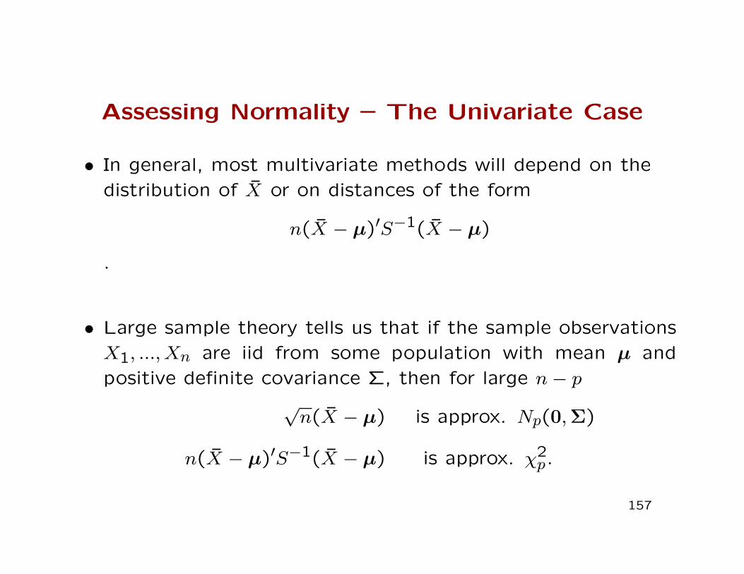
Assessing Normality – The Univariate Case • In general, most multivariate methods will depend on the distribution of ¯ X or on distances of the form n( ¯ X - μ) 0 S -1 ( ¯ X - μ) . • Large sample theory tells us that if the sample observations X 1 , ..., X n are iid from some population with mean μ and positive definite covariance Σ, then for large n - p √ n( ¯ X - μ) is approx. N p (0, Σ) n( ¯ X - μ) 0 S -1 ( ¯ X - μ) is approx. χ 2 p . 157
-
Upload
truongdung -
Category
Documents
-
view
237 -
download
0
Transcript of Assessing Normality { The Univariate Casemaitra/stat501/lectures/AssessingNormality.pdf ·...
Assessing Normality – The Univariate Case
• In general, most multivariate methods will depend on the
distribution of X or on distances of the form
n(X − µ)′S−1(X − µ)
.
• Large sample theory tells us that if the sample observations
X1, ..., Xn are iid from some population with mean µ and
positive definite covariance Σ, then for large n− p√n(X − µ) is approx. Np(0,Σ)
n(X − µ)′S−1(X − µ) is approx. χ2p .
157
Assessing Normality (cont’d)
• This holds regardless of the form of the distribution of the
observations.
• In making inferences about mean vectors, it is not crucial to
begin with MVN observations if samples are large enough.
• For small samples, we will need to check if observations were
sampled from a multivariate normal population
158
Assessing Normality (cont’d)
• Assessing multivariate normality is difficult in highdimensions.
• We first focus on the univariate marginals, the bivariatemarginals, and the behavior of other sample quantities. Inparticular:
1. Do the marginals appear to be normal?
2. Do scatter plots of pairs of observations have an ellipticalshape?
3. Are there ’wild’observations?
4. Do the ellipsoids ’contain’ something close to the ex-pected number of observations?
159
Assessing Normality (cont’d)
• One other approach to check normality is to investigate thebehavior of conditional means and variances. If X1, X2 arejointly normal, then
1. The conditional means E(X1|X2) and E(X2|X1) arelinear functions of the conditioning variable.
2. The conditional variances do not depend on theconditioning variables.
• Even if all the answers to questions appear to suggestunivariate or bivariate normality, we cannot conclude thatthe sample arose from a MVN normal distribution.
160
Assessing Normality (cont’d)
• If X ∼MVN , all the marginals are normal, but the converseis not necessarily true. Further, if X ∼MVN , then the condi-tionals are also normal, but the converse does not necessarilyfollow.
• In general, then, we will be checking whether necessary butnot sufficient conditions for multivariate normality hold ornot.
• Most investigations in the book use univariate normality, butwe are also going to present some practical and recent workon assessing multivariate normality.
161
Univariate Normal Distribution
• If X ∼ N(µ, σ2), we know that
Probability for interval (µ−√σ2, µ+
√σ2) ≈ 0.68
Probability for interval (µ− 2√σ2, µ+ 2
√σ2) ≈ 0.95
Probability for interval (µ− 3√σ2, µ+ 3
√σ2) ≈ 0.99.
• In moderately large samples, we can count the proportion ofobservations that appear to fall in the corresponding inter-vals where sample means and variances have been pluggedin place of the population parameters.
• We can implement this simple approach for each of our p
variables.
162
Normal Q-Q plots
• Quantile-quantile plots can also be constructed for each of
the p variables.
• In a Q-Q plot, we plot the sample quantiles against the
quantiles that would be expected if the sample came from a
standard normal distribution.
• If the hypothesis of normality holds, the points in the plot
will fall along a straight line.
163
Normal Q-Q plots
• The slope of the estimated line is an estimate of the popu-lation standard deviation.
• The intercept of the estimated line is an estimate of thepopulation mean.
• The sample quantiles are just the sample order statistics.For a sample x1, x2, ..., xn, quantiles are obtained by orderingsample observations
x(1) ≤ x(2) ≤ ... ≤ x(n),
where x(j) is the jth smallest sample observation or the jthsample order statistic.
164
Normal Q-Q plots (cont’d)
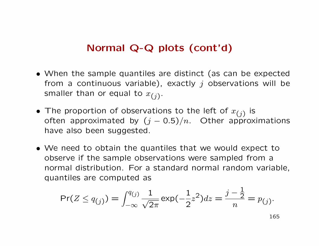
• When the sample quantiles are distinct (as can be expectedfrom a continuous variable), exactly j observations will besmaller than or equal to x(j).
• The proportion of observations to the left of x(j) isoften approximated by (j − 0.5)/n. Other approximationshave also been suggested.
• We need to obtain the quantiles that we would expect toobserve if the sample observations were sampled from anormal distribution. For a standard normal random variable,quantiles are computed as
Pr(Z ≤ q(j)) =∫ q(j)
−∞
1√2π
exp(−1
2z2)dz =
j − 12
n= p(j).
165
Normal Q-Q plots (cont’d)
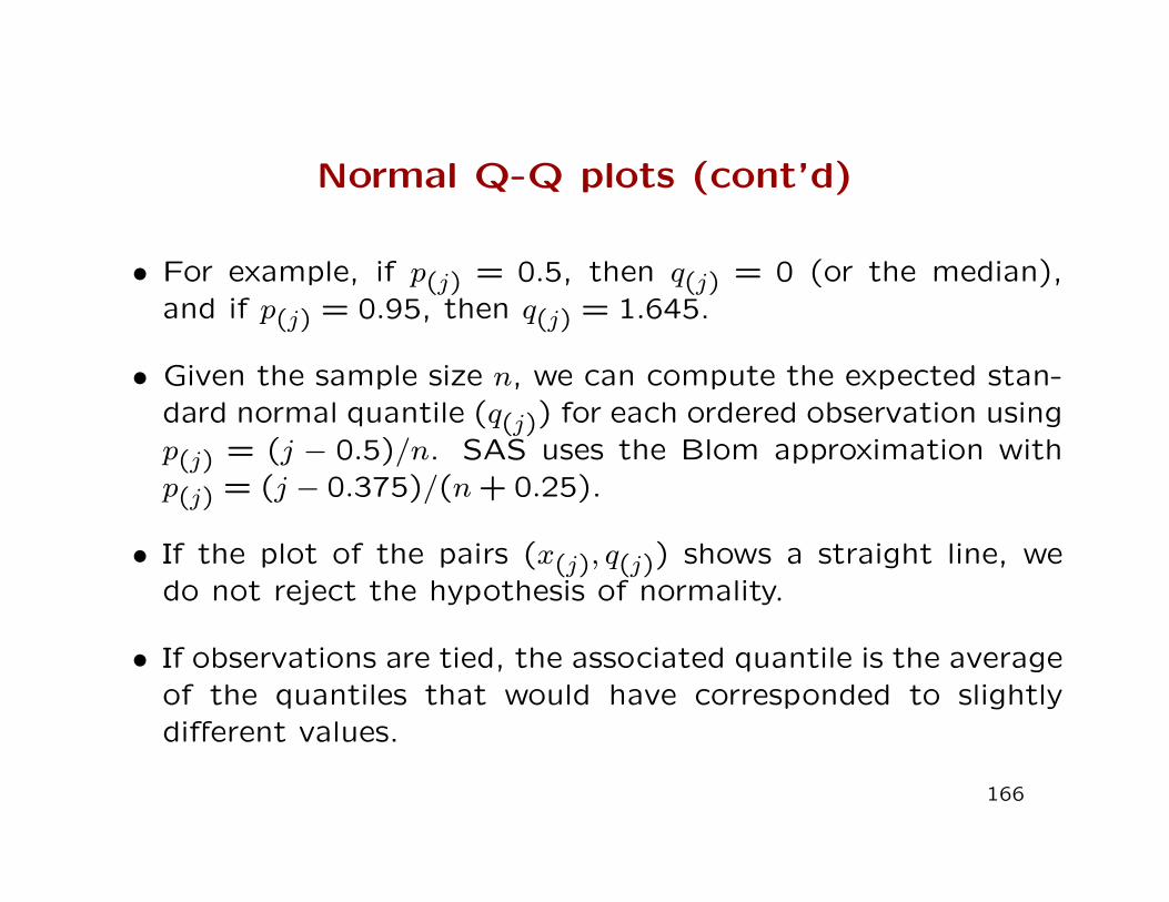
• For example, if p(j) = 0.5, then q(j) = 0 (or the median),and if p(j) = 0.95, then q(j) = 1.645.
• Given the sample size n, we can compute the expected stan-dard normal quantile (q(j)) for each ordered observation usingp(j) = (j − 0.5)/n. SAS uses the Blom approximation withp(j) = (j − 0.375)/(n+ 0.25).
• If the plot of the pairs (x(j), q(j)) shows a straight line, wedo not reject the hypothesis of normality.
• If observations are tied, the associated quantile is the averageof the quantiles that would have corresponded to slightlydifferent values.
166
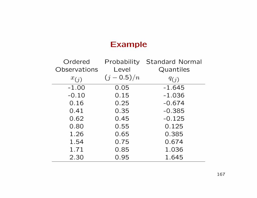
Example
Ordered Probability Standard NormalObservations Level Quantiles
x(j) (j − 0.5)/n q(j)
-1.00 0.05 -1.645-0.10 0.15 -1.0360.16 0.25 -0.6740.41 0.35 -0.3850.62 0.45 -0.1250.80 0.55 0.1251.26 0.65 0.3851.54 0.75 0.6741.71 0.85 1.0362.30 0.95 1.645
167
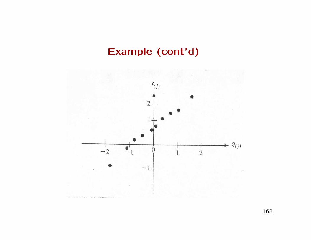
Example (cont’d)
168
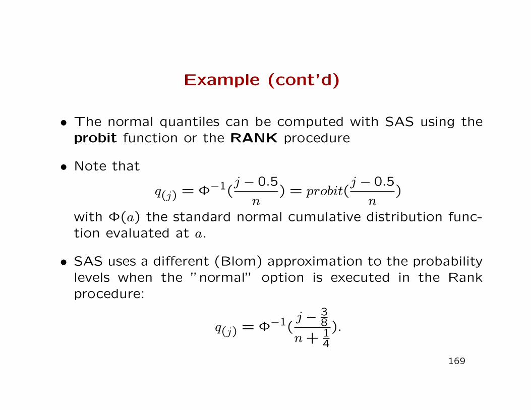
Example (cont’d)
• The normal quantiles can be computed with SAS using theprobit function or the RANK procedure
• Note that
q(j) = Φ−1(j − 0.5
n) = probit(
j − 0.5
n)
with Φ(a) the standard normal cumulative distribution func-tion evaluated at a.
• SAS uses a different (Blom) approximation to the probabilitylevels when the ”normal” option is executed in the Rankprocedure:
q(j) = Φ−1(j − 3
8
n+ 14
).
169
Microwave ovens: Example 4.10
• Microwave ovens are required by the federal governmentto emit less than a certain amount of radiation when thedoors are closed.
• Manufacturers regularly monitor compliance with theregulation by estimating the probability that a randomlychosen sample of ovens from the production line exceedthe tolerance level.
• Is the assumption of normality adequate when estimatingthe probability?
• A sample of n = 42 ovens were obtained (see Table 4.1,page 180). To assess whether the assumption of normalityis plausible, a Q-Q plot was constructed.
170
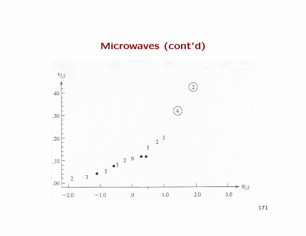
Microwaves (cont’d)
171
Goodness of Fit TestsCorrelation Test
• In addition to visual inspection, we can compute the
correlation between the x(j) and the q(j):
rQ =
∑ni=1(x(i) − x)(q(i) − q)√∑n
i=1(x(i) − x)2√∑n
i=1(q(i) − q)2.
• We expect values of rQ close to one if the sample arises from
a normal population.
• Note that q = 0, so the above expression simplifies.
172
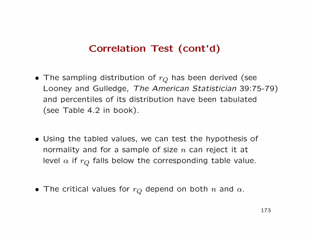
Correlation Test (cont’d)
• The sampling distribution of rQ has been derived (see
Looney and Gulledge, The American Statistician 39:75-79)
and percentiles of its distribution have been tabulated
(see Table 4.2 in book).
• Using the tabled values, we can test the hypothesis of
normality and for a sample of size n can reject it at
level α if rQ falls below the corresponding table value.
• The critical values for rQ depend on both n and α.
173
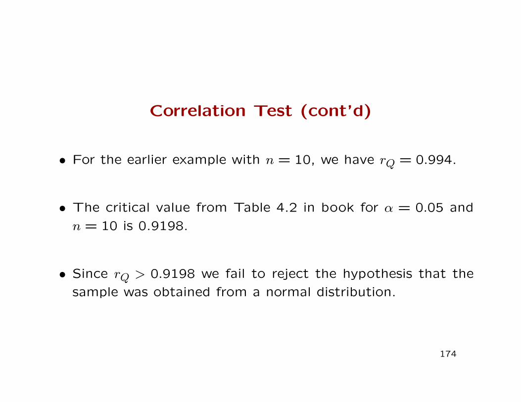
Correlation Test (cont’d)
• For the earlier example with n = 10, we have rQ = 0.994.
• The critical value from Table 4.2 in book for α = 0.05 and
n = 10 is 0.9198.
• Since rQ > 0.9198 we fail to reject the hypothesis that the
sample was obtained from a normal distribution.
174
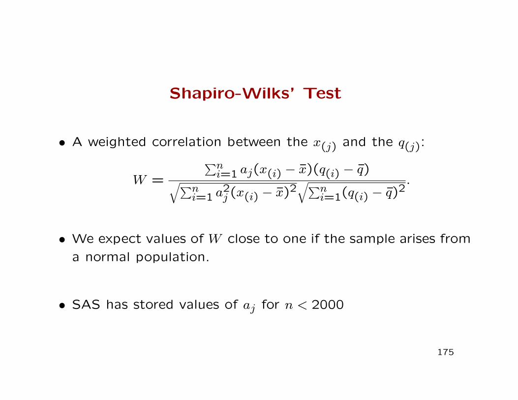
Shapiro-Wilks’ Test
• A weighted correlation between the x(j) and the q(j):
W =
∑ni=1 aj(x(i) − x)(q(i) − q)√∑n
i=1 a2j (x(i) − x)2
√∑ni=1(q(i) − q)2
.
• We expect values of W close to one if the sample arises from
a normal population.
• SAS has stored values of aj for n < 2000
175
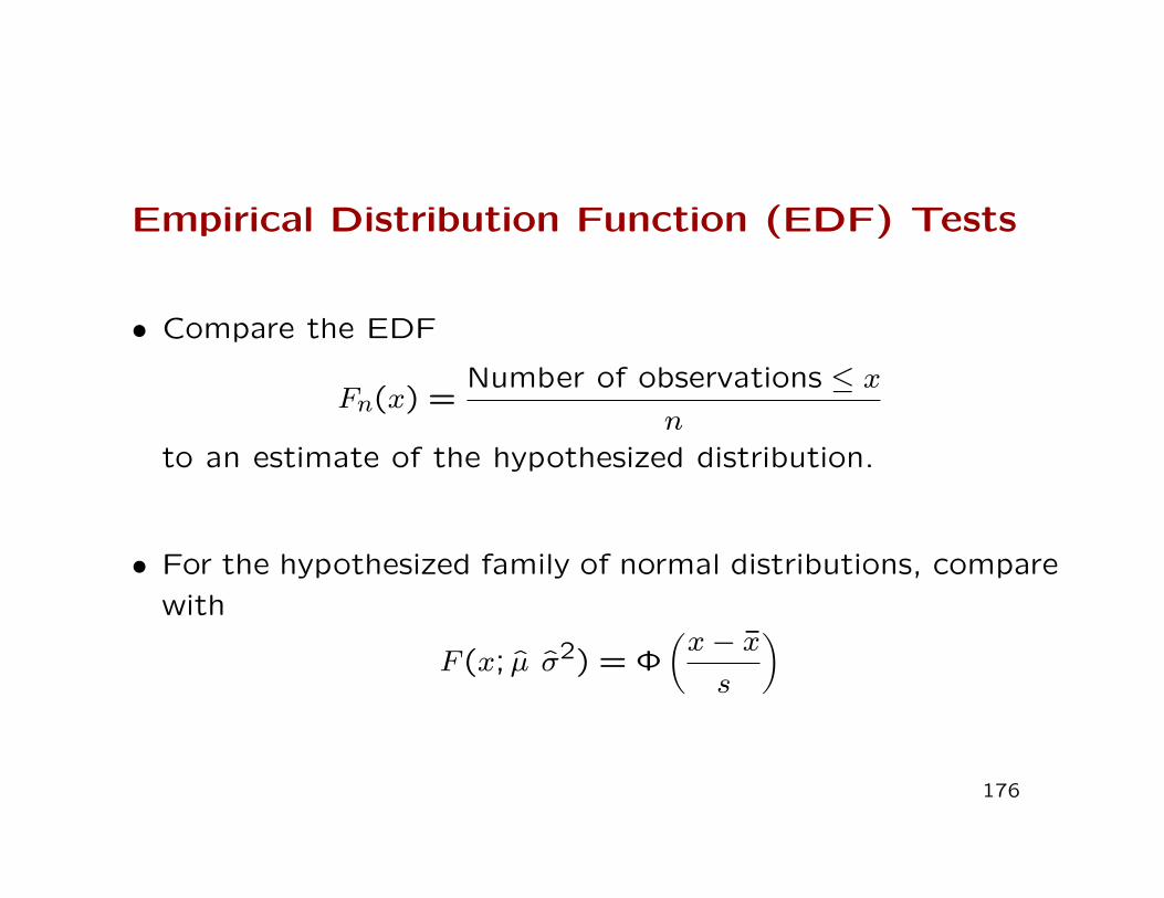
Empirical Distribution Function (EDF) Tests
• Compare the EDF
Fn(x) =Number of observations ≤ x
n
to an estimate of the hypothesized distribution.
• For the hypothesized family of normal distributions, compare
with
F (x; µ σ2) = Φ(x− xs
)
176
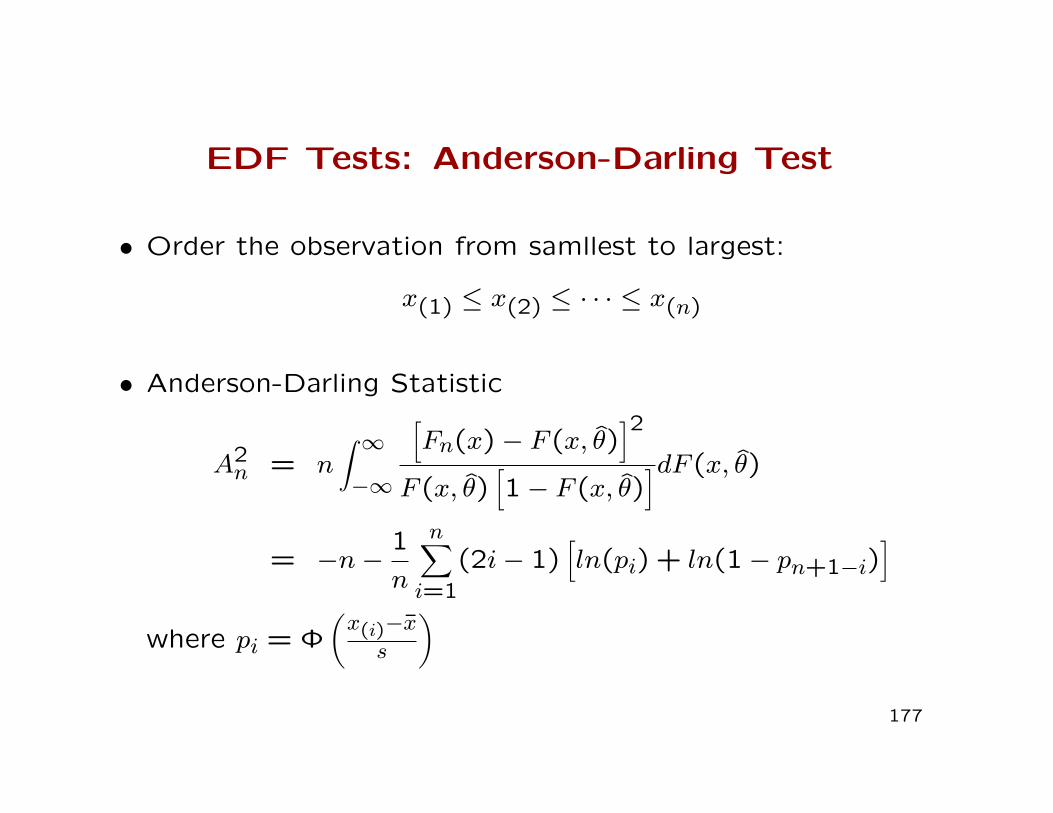
EDF Tests: Anderson-Darling Test
• Order the observation from samllest to largest:
x(1) ≤ x(2) ≤ · · · ≤ x(n)
• Anderson-Darling Statistic
A2n = n
∫ ∞−∞
[Fn(x)− F (x, θ)
]2F (x, θ)
[1− F (x, θ)
]dF (x, θ)
= −n−1
n
n∑i=1
(2i− 1)[ln(pi) + ln(1− pn+1−i)
]where pi = Φ
(x(i)−xs
)
177

EDF Tests: Kolmogorov-Smirnov Test
• Order the observation from samllest to largest:
x(1) ≤ x(2) ≤ · · · ≤ x(n)
• Kolmogorov-Smirnov Statistic
Dn = max(D−, D+
)where D−n = max1≤i≤n
∣∣∣pi − i−1n
∣∣∣ and D+n = max1≤i≤n
∣∣∣pi − in
∣∣∣and pi = Φ
(x(i)−xs
)
178
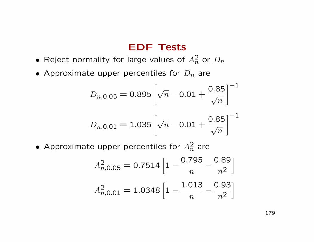
EDF Tests• Reject normality for large values of A2
n or Dn
• Approximate upper percentiles for Dn are
Dn,0.05 = 0.895
[√n− 0.01 +
0.85√n
]−1
Dn,0.01 = 1.035
[√n− 0.01 +
0.85√n
]−1
• Approximate upper percentiles for A2n are
A2n,0.05 = 0.7514
[1−
0.795
n−
0.89
n2
]
A2n,0.01 = 1.0348
[1−
1.013
n−
0.93
n2
]
179
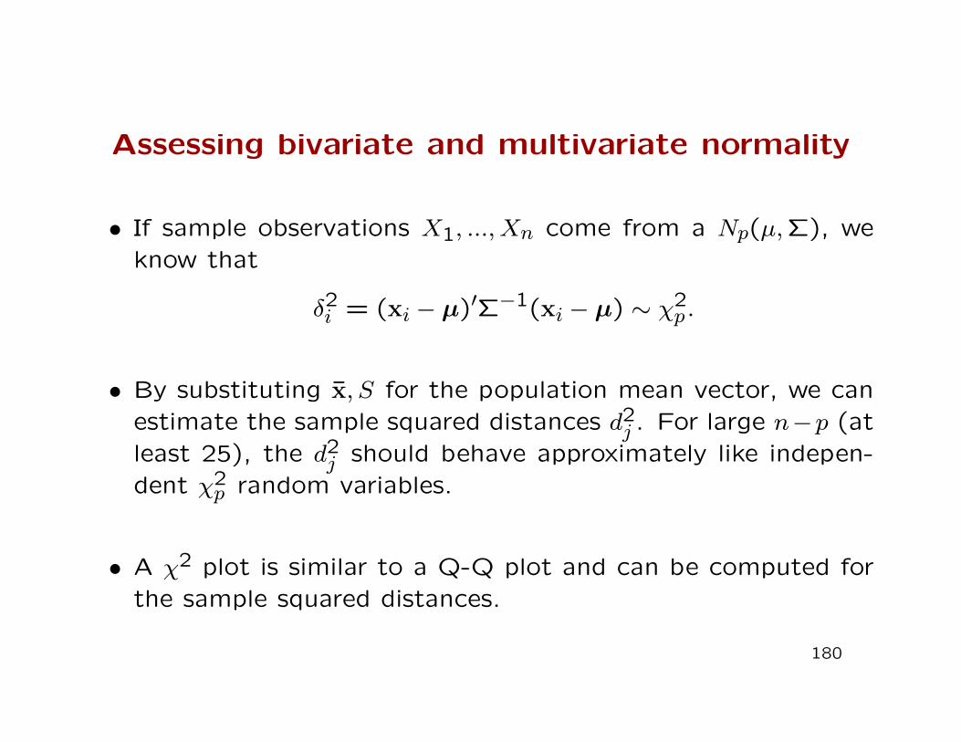
Assessing bivariate and multivariate normality
• If sample observations X1, ..., Xn come from a Np(µ,Σ), weknow that
δ2i = (xi − µ)′Σ−1(xi − µ) ∼ χ2
p .
• By substituting x, S for the population mean vector, we canestimate the sample squared distances d2
j . For large n−p (atleast 25), the d2
j should behave approximately like indepen-dent χ2
p random variables.
• A χ2 plot is similar to a Q-Q plot and can be computed forthe sample squared distances.
180
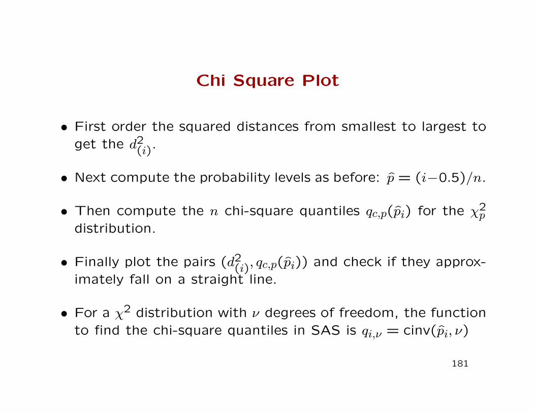
Chi Square Plot
• First order the squared distances from smallest to largest toget the d2
(i).
• Next compute the probability levels as before: p = (i−0.5)/n.
• Then compute the n chi-square quantiles qc,p(pi) for the χ2p
distribution.
• Finally plot the pairs (d2(i), qc,p(pi)) and check if they approx-
imately fall on a straight line.
• For a χ2 distribution with ν degrees of freedom, the functionto find the chi-square quantiles in SAS is qi,ν = cinv(pi, ν)
181
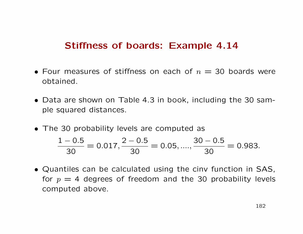
Stiffness of boards: Example 4.14
• Four measures of stiffness on each of n = 30 boards wereobtained.
• Data are shown on Table 4.3 in book, including the 30 sam-ple squared distances.
• The 30 probability levels are computed as
1− 0.5
30= 0.017,
2− 0.5
30= 0.05, ....,
30− 0.5
30= 0.983.
• Quantiles can be calculated using the cinv function in SAS,for p = 4 degrees of freedom and the 30 probability levelscomputed above.
182

Example (cont’d)
183
Formal Tests for Multivariate Normality - I
• For any X, we have seen that X ∼MVN iff a′X is univariate
normally distributed.
• How about taking a large (but random) number of projec-
tions and evaluating each projection for univariate normality?
• Let us try with N (large, random) independent random pro-
jections on the unit vector. We will test each projection for
univariate normality using the Shapiro-Wilks’ test.
184
Formal Tests for Multivariate Normality - I(contd.)
• Note that we will have a large number of tests to evaluate,and this means that we will have to account for multiplehypothesis tests that have to be carried out. So we convertall the p-values into so-called q-values and if all the q-valuesare greater than the desired False Discovery Rate (FDR),then we accept the null hypothesis that X is multivariatenormally distributed.
• Note the large number of calculations needed: imperative towrite R code efficiently.
– code provided in testnormality.R.
185

The Energy Test for Multivariate Normality
• Let X1,X2, . . . ,Xn be a sample from some p-variate distribu-tion. Then, consider the following “energy” test statistic:
E = n
2
n
n∑i=1
IE ‖ X∗i − Z ‖ −IE ‖ Z− Z′ ‖ −1
n2
n∑i=1
‖ X∗i −X∗j ‖
,where X∗i , i = 1,2, . . . , n is the standardized sample and Z, andZ′ are independent identically distributed p-variate standardnormal random vectors, and ‖ · ‖ denotes Euclidean norm.
• The critical region is obtain by parametric bootstrap.
• Implemented in R by the mvnorm.etest() function in the energy
package also provided by authors Szekely and Rizzo (2005).
186
Detecting Outliers
• An outlier is a measurement that appears to be muchdifferent from neighboring observations.
• In the univariate case with adequate sample sizes, andassuming that normality holds, an outlier can bedetected by:
1. Standardizing the n measurements so that theyare approximately N(0.1).
2. Flagging observations with standardized values belowor above 3.5 or thereabouts.
• In p dimensions, detecting outliers is not so easy. A sampleunit which may not appear to be an outlier in each of themarginal distributions, can still be an outlier relative to themultivariate distribution.
187
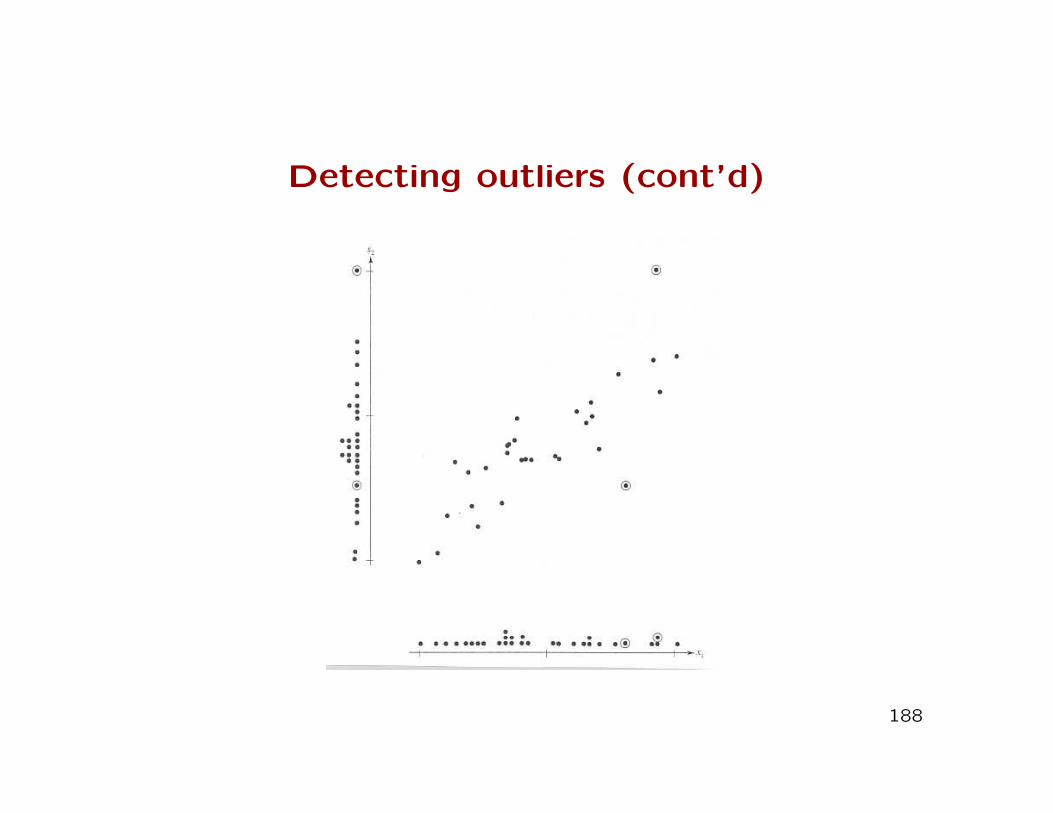
Detecting outliers (cont’d)
188
Steps for detecting outliers
1. Investigate all univariate marginal distributions, visually byconstructing the standardized values zij = (xij − x)/√σjj forthe i-th sample unit and j-th variable.
2. If p is moderate, construct all bivariate scatter plots. Thereare p(p− 1)/2 of them.
3. For each sample unit, calculate the squared distanced2i = (xi − x)′S−1(xi − x), where xi is the p× 1 vector of
measurements on the i-th sample unit.
4. To decide if d2i is ’extreme’, recall that the d2
i areapproximately χ2
p. For example, if n = 100, we wouldexpect to observe about 5 squared distances larger thanthe 0.95 percentile of the χ2
p distribution.
189
Example: Stiffness of lumber boards
• Recall that four measurements were taken on each of 30boards.
• Data are shown in Table 4.4 along with the four columns ofstandardized values and the 30 squared distances.
• Note that boards 9 and 16 have unusually large d2, of 12.26and 16.85, respectively. The 0.975 and 0.995 percentiles ofa χ2
4 distribution are 11.14 and 14.86.
• In a sample of size 30, we would expect less than 0.75 obs.with d2 > 11.14 and less than 0.015 obs. with d2 > 14.86.
• Unit 16, with d2 = 16.85 is not flagged as an outlier whenwe only consider the univariate standardized measurements.
190
Detecting if Outliers are Present
• Mardia’s (1970, 1974, 1975) multivariate sample kurtosis
measure
b2,p(X) = n−1n∑i=1
(Xi − X)′S−1(Xi − X). (1)
• Schwager and Margolin (1982) have shown that the pres-
ence of multivariate outliers can be ascertained, if b2,p(X) is
greater than some cut-off.
191
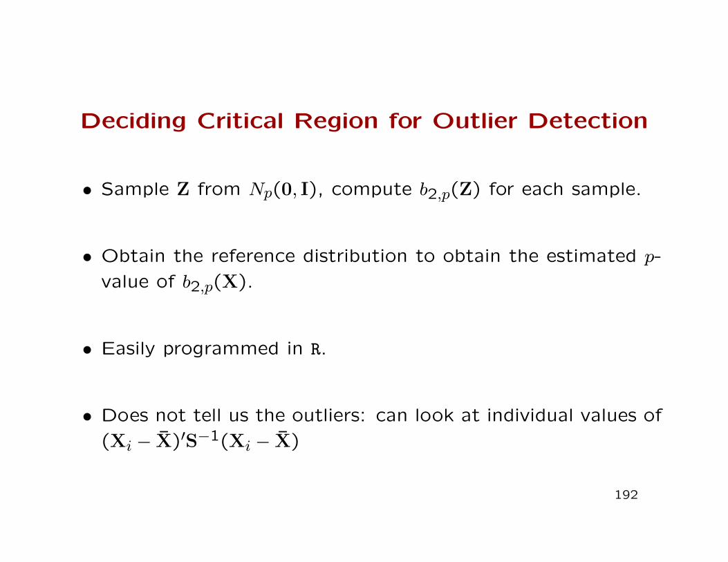
Deciding Critical Region for Outlier Detection
• Sample Z from Np(0, I), compute b2,p(Z) for each sample.
• Obtain the reference distribution to obtain the estimated p-
value of b2,p(X).
• Easily programmed in R.
• Does not tell us the outliers: can look at individual values of
(Xi − X)′S−1(Xi − X)
192
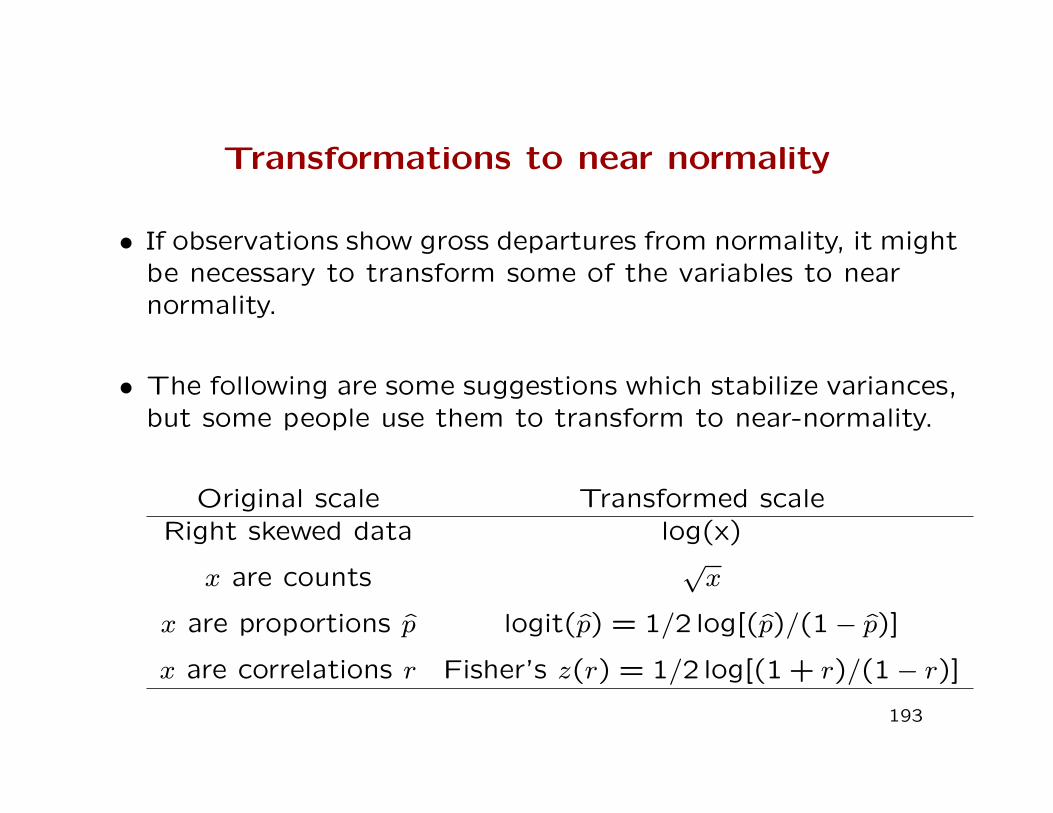
Transformations to near normality
• If observations show gross departures from normality, it mightbe necessary to transform some of the variables to nearnormality.
• The following are some suggestions which stabilize variances,but some people use them to transform to near-normality.
Original scale Transformed scaleRight skewed data log(x)
x are counts√x
x are proportions p logit(p) = 1/2 log[(p)/(1− p)]
x are correlations r Fisher’s z(r) = 1/2 log[(1 + r)/(1− r)]
193
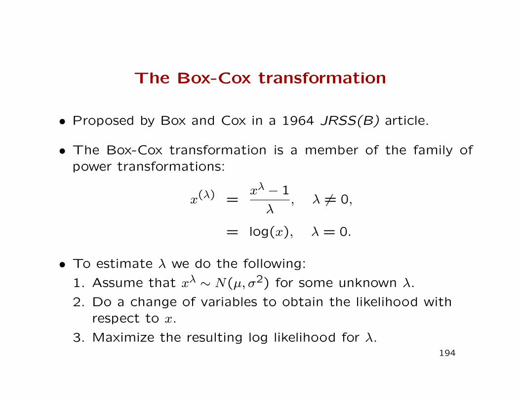
The Box-Cox transformation
• Proposed by Box and Cox in a 1964 JRSS(B) article.
• The Box-Cox transformation is a member of the family ofpower transformations:
x(λ) =xλ − 1
λ, λ 6= 0,
= log(x), λ = 0.
• To estimate λ we do the following:
1. Assume that xλ ∼ N(µ, σ2) for some unknown λ.
2. Do a change of variables to obtain the likelihood withrespect to x.
3. Maximize the resulting log likelihood for λ.194
Box-Cox Transformation (cont’d)
• If xλ ∼ N(µ, σ2), then with respect to the untransformedobservations the resulting log-likelihood is
L(µ, σ2, λ) = −n
2log(2πσ2)−
1
2σ2
n∑i=1
(x(λ)i −µ)2+(λ−1)
n∑i=1
log(xi),
where the last term is the logarithm of the Jacobian of thetransformation |dxλi /dxi|.
• Substituting MLEs for µ and σ2 we get, as a function of λalone:
l(λ) = −n
2[1
n
∑i
(x(λ)i − ¯x(λ))2] + (λ− 1)
∑i
log(xi).
• The best power transformation λ is the one that maximizesthe expression above.
195
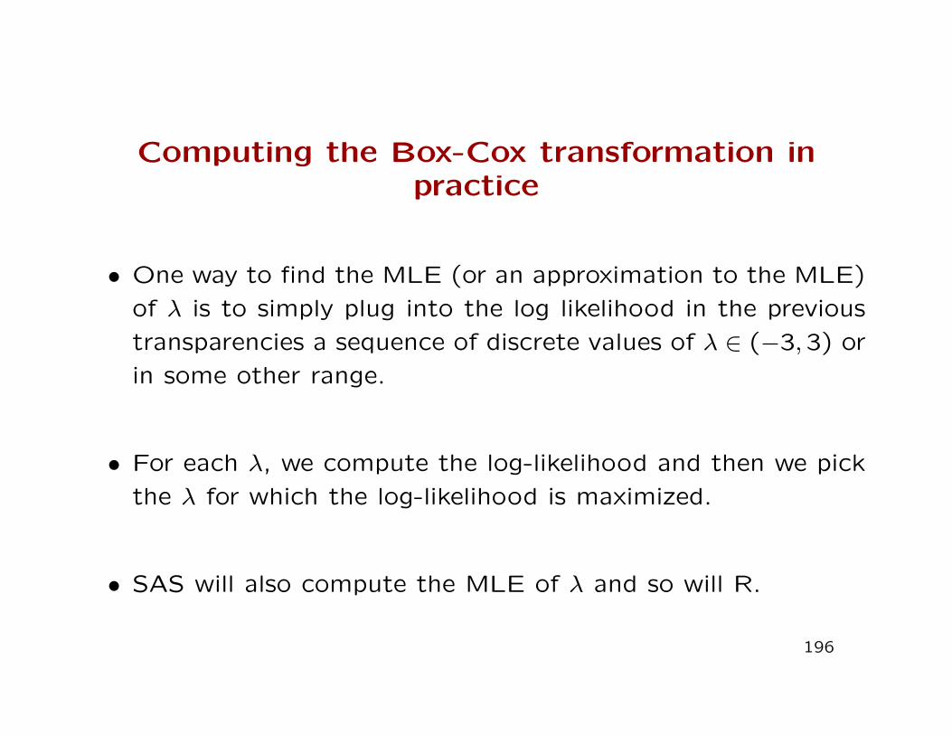
Computing the Box-Cox transformation inpractice
• One way to find the MLE (or an approximation to the MLE)
of λ is to simply plug into the log likelihood in the previous
transparencies a sequence of discrete values of λ ∈ (−3,3) or
in some other range.
• For each λ, we compute the log-likelihood and then we pick
the λ for which the log-likelihood is maximized.
• SAS will also compute the MLE of λ and so will R.
196
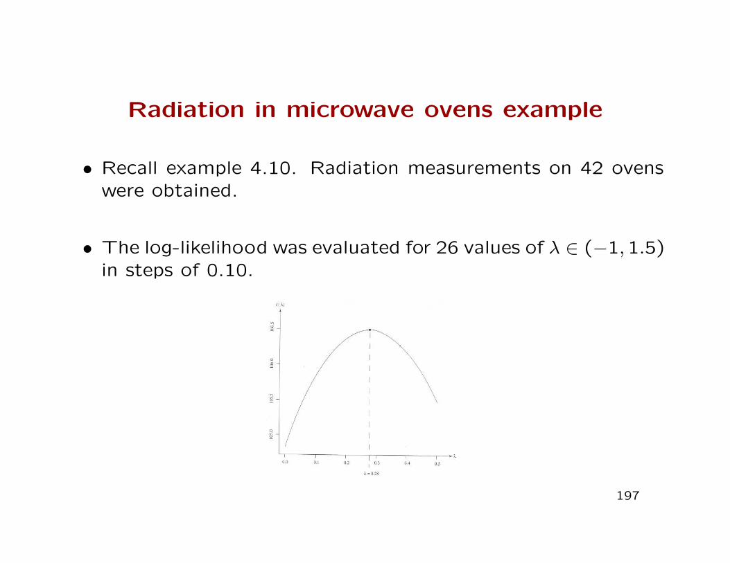
Radiation in microwave ovens example
• Recall example 4.10. Radiation measurements on 42 ovenswere obtained.
• The log-likelihood was evaluated for 26 values of λ ∈ (−1,1.5)in steps of 0.10.
197
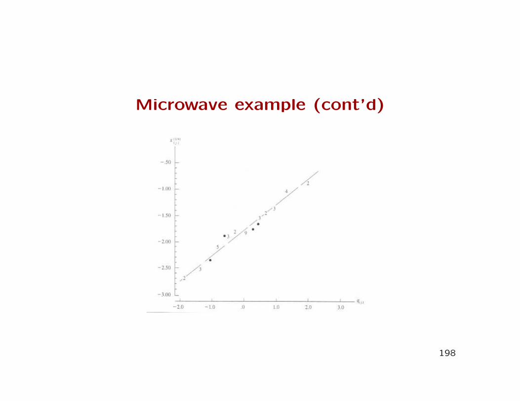
Microwave example (cont’d)
198
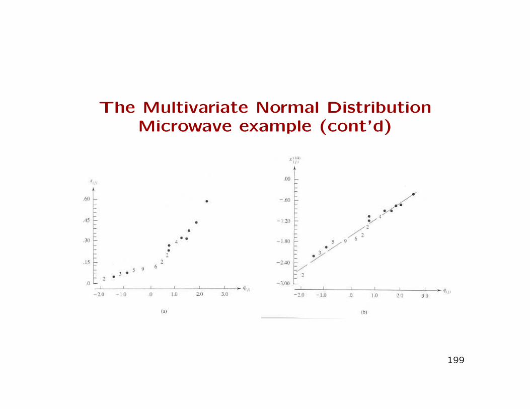
The Multivariate Normal DistributionMicrowave example (cont’d)
199
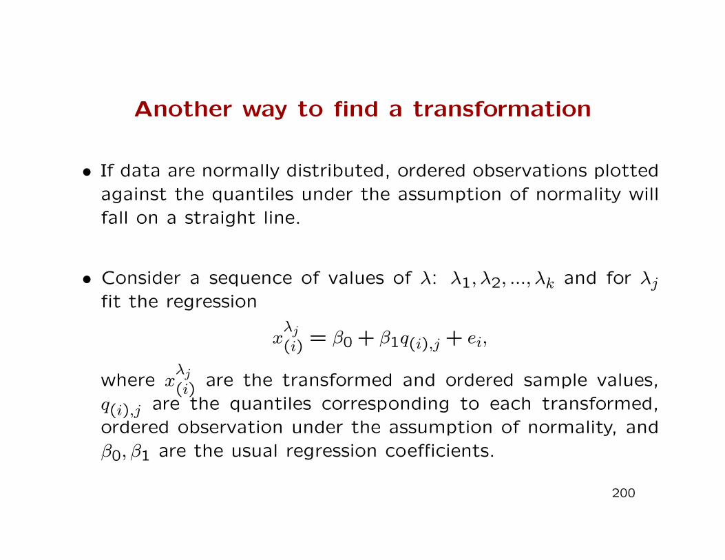
Another way to find a transformation
• If data are normally distributed, ordered observations plottedagainst the quantiles under the assumption of normality willfall on a straight line.
• Consider a sequence of values of λ: λ1, λ2, ..., λk and for λjfit the regression
xλj(i) = β0 + β1q(i),j + ei,
where xλj(i) are the transformed and ordered sample values,
q(i),j are the quantiles corresponding to each transformed,ordered observation under the assumption of normality, andβ0, β1 are the usual regression coefficients.
200
Alternative estimation method (cont’d)
• For each of the k regressions (one for each λj), compute the
MSE.
• The best fitting model will have lowest MSE.
• Therefore, the λ which minimizes the MSE of the regression
of sample quantiles on normal quantiles will be ’best’.
• It can be shown that this is also the λ that maximizes the
log-likelihood function shown earlier.
201
Transforming multivariate observations
• By transforming each of the p measurements individually, we
approximate normality of the marginals but not necessarily
of the joint p-dimensional distribution.
• It is possible to proceed as in the Box-Cox approach and try
to maximize the log-likelihood jointly for all p lambdas. This
is called the multivariate Box-Cox transform.
202
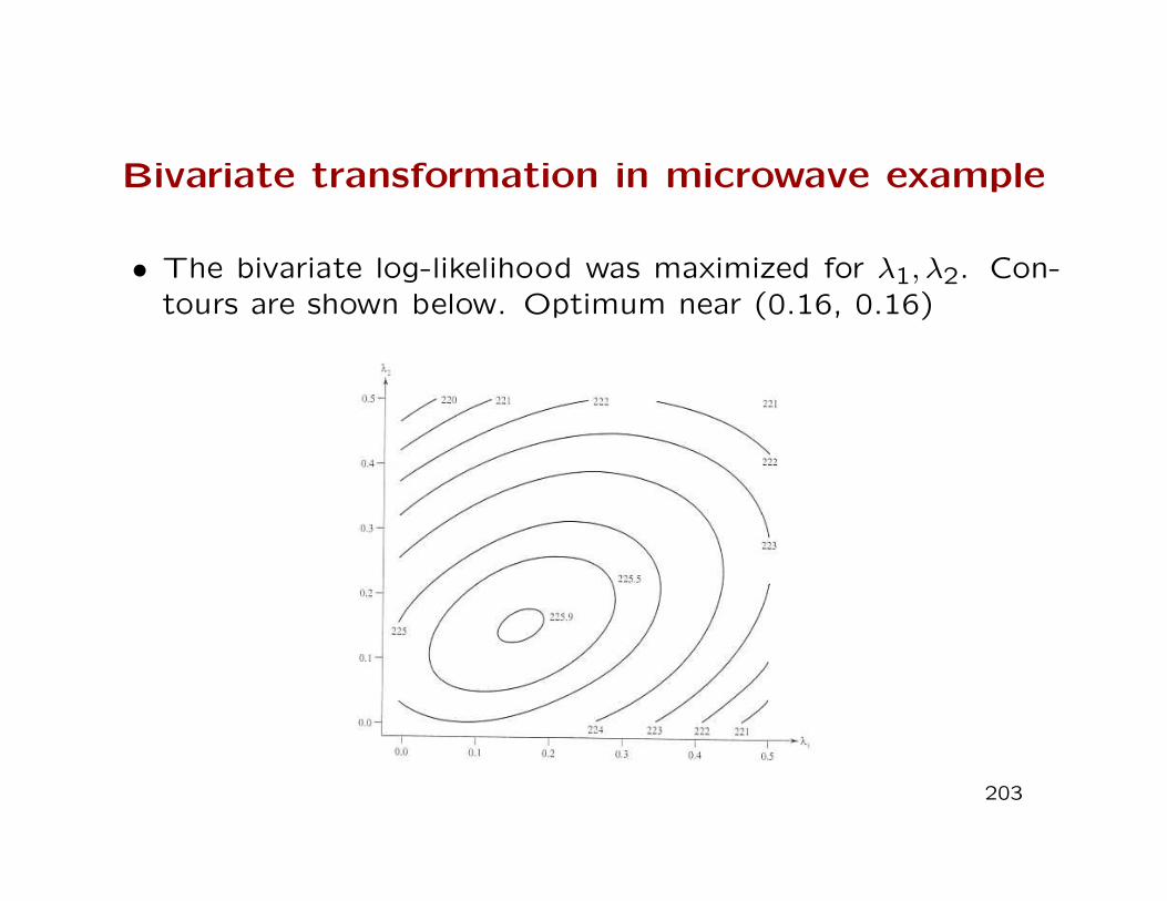
Bivariate transformation in microwave example
• The bivariate log-likelihood was maximized for λ1, λ2. Con-tours are shown below. Optimum near (0.16, 0.16)
203


![Assessing Cellular Response to Functionalized α-Helical ...two-component peptide system for making hydrogels, termed hSAFs (hydrogelating self-assembling fi bers). [ 32 ] The peptides](https://static.fdocument.org/doc/165x107/60df4feff816521c5855918c/assessing-cellular-response-to-functionalized-helical-two-component-peptide.jpg)