arX

iv:h

ep-t

h/92

1007

3 v1

14

Oct

199

2ITD 92/92–10

Introduction to Random Matrices

Craig A. Tracy

Department of Mathematics and Institute of Theoretical Dynamics,

University of California, Davis, CA 95616, USA

Harold WidomDepartment of Mathematics,

University of California, Santa Cruz, CA 95064, USA

These notes provide an introduction to the theory of random matrices. The central quantitystudied is τ (a) = det (1 − K) where K is the integral operator with kernel

1

π

sin π(x − y)

x − yχI(y) .

Here I =⋃

j(a2j−1, a2j) and χI(y) is the characteristic function of the set I . In the Gaussian

Unitary Ensemble (GUE) the probability that no eigenvalues lie in I is equal to τ (a). Also τ (a)is a tau-function and we present a new simplified derivation of the system of nonlinear completelyintegrable equations (the aj ’s are the independent variables) that were first derived by Jimbo, Miwa,Mori, and Sato in 1980. In the case of a single interval these equations are reducible to a PainleveV equation. For large s we give an asymptotic formula for E2(n; s), which is the probability in theGUE that exactly n eigenvalues lie in an interval of length s.

I. INTRODUCTION

These notes provide an introduction to that aspect of the theory of random matrices dealing with the distributionof eigenvalues. To first orient the reader, we present in Sec. II some numerical experiments that illustrate some ofthe basic aspects of the subject. In Sec. III we introduce the invariant measures for the three “circular ensembles”involving unitary matrices. We also define the level spacing distributions and express these distributions in terms of aparticular Fredholm determinant. In Sec. IV we explain how these measures are modified for the orthogonal polynomialensembles. In Sec. V we discuss the universality of these level spacing distribution functions in a particular scalinglimit. The discussion up to this point (with the possible exception of Sec. V) follows the well-known path pioneeredby Hua, Wigner, Dyson, Mehta and others who first developed this theory (see, e.g., the reprint volume of Porter [34]and Hua [17]). This, and much more, is discussed in Mehta’s book [25]—the classic reference in the subject.

An important development in random matrices was the discovery by Jimbo, Miwa, Mori, and Sato [21] (hereafterreferred to as JMMS) that the basic Fredholm determinant mentioned above is a τ -function in the sense of the KyotoSchool. Though it has been some twelve years since [21] was published, these results are not widely appreciated bythe practitioners of random matrices. This is due no doubt to the complexity of their paper. The methods of JMMSare methods of discovery; but now that we know the result, simpler proofs can be constructed. In Sec. VI we givesuch a proof of the JMMS equations. Our proof is a simplification and generalization of Mehta’s [27] simplified proofof the single interval case. Also our methods build on the earlier work of Its, Izergin, Korepin, and Slavnov [18] andDyson [12]. We include in this section a discussion of the connection between the JMMS equations and the integrableHamiltonian systems that appear in the geometry of quadrics and spectral theory as developed by Moser [31]. Thissection concludes with a discussion of the case of a single interval (viz., probability that exactly n eigenvalues lie ina given interval). In this case the JMMS equations can be reduced to a single ordinary differential equation—thePainleve V equation.

Finally, in Sec. VII we discuss the asymptotics in the case of a large single interval of the various level spacingdistribution functions [4,38,28]. In this analysis both the Painleve representation and new results in Toeplitz/Wiener-Hopf theory are needed to produce these asymptotics. We also give an approach based on the asymptotics of theeigenvalues of the basic linear integral operator [14,25,35]. These results are then compared with the continuum modelcalculations of Dyson [12].

1

II. NUMERICAL EXPERIMENTS

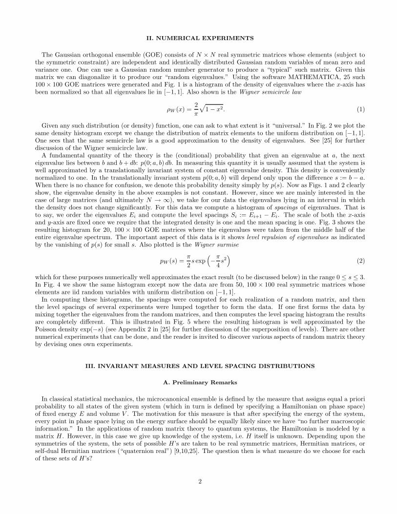
The Gaussian orthogonal ensemble (GOE) consists of N × N real symmetric matrices whose elements (subject tothe symmetric constraint) are independent and identically distributed Gaussian random variables of mean zero andvariance one. One can use a Gaussian random number generator to produce a “typical” such matrix. Given thismatrix we can diagonalize it to produce our “random eigenvalues.” Using the software MATHEMATICA, 25 such100 × 100 GOE matrices were generated and Fig. 1 is a histogram of the density of eigenvalues where the x-axis hasbeen normalized so that all eigenvalues lie in [−1, 1]. Also shown is the Wigner semicircle law

ρW (x) =2

π

√

1 − x2. (1)

Given any such distribution (or density) function, one can ask to what extent is it “universal.” In Fig. 2 we plot thesame density histogram except we change the distribution of matrix elements to the uniform distribution on [−1, 1].One sees that the same semicircle law is a good approximation to the density of eigenvalues. See [25] for furtherdiscussion of the Wigner semicircle law.

A fundamental quantity of the theory is the (conditional) probability that given an eigenvalue at a, the nexteigenvalue lies between b and b + db: p(0; a, b) db. In measuring this quantity it is usually assumed that the system iswell approximated by a translationally invariant system of constant eigenvalue density. This density is convenientlynormalized to one. In the translationally invariant system p(0; a, b) will depend only upon the difference s := b − a.When there is no chance for confusion, we denote this probability density simply by p(s). Now as Figs. 1 and 2 clearlyshow, the eigenvalue density in the above examples is not constant. However, since we are mainly interested in thecase of large matrices (and ultimately N → ∞), we take for our data the eigenvalues lying in an interval in whichthe density does not change significantly. For this data we compute a histogram of spacings of eigenvalues. That isto say, we order the eigenvalues Ei and compute the level spacings Si := Ei+1 − Ei. The scale of both the x-axisand y-axis are fixed once we require that the integrated density is one and the mean spacing is one. Fig. 3 shows theresulting histogram for 20, 100 × 100 GOE matrices where the eigenvalues were taken from the middle half of theentire eigenvalue spectrum. The important aspect of this data is it shows level repulsion of eigenvalues as indicatedby the vanishing of p(s) for small s. Also plotted is the Wigner surmise

pW (s) =π

2s exp

(

−π

4s2

)

(2)

which for these purposes numerically well approximates the exact result (to be discussed below) in the range 0 ≤ s ≤ 3.In Fig. 4 we show the same histogram except now the data are from 50, 100 × 100 real symmetric matrices whoseelements are iid random variables with uniform distribution on [−1, 1].

In computing these histograms, the spacings were computed for each realization of a random matrix, and thenthe level spacings of several experiments were lumped together to form the data. If one first forms the data bymixing together the eigenvalues from the random matrices, and then computes the level spacing histogram the resultsare completely different. This is illustrated in Fig. 5 where the resulting histogram is well approximated by thePoisson density exp(−s) (see Appendix 2 in [25] for further discussion of the superposition of levels). There are othernumerical experiments that can be done, and the reader is invited to discover various aspects of random matrix theoryby devising ones own experiments.

III. INVARIANT MEASURES AND LEVEL SPACING DISTRIBUTIONS

A. Preliminary Remarks

In classical statistical mechanics, the microcanonical ensemble is defined by the measure that assigns equal a prioriprobability to all states of the given system (which in turn is defined by specifying a Hamiltonian on phase space)of fixed energy E and volume V . The motivation for this measure is that after specifying the energy of the system,every point in phase space lying on the energy surface should be equally likely since we have “no further macroscopicinformation.” In the applications of random matrix theory to quantum systems, the Hamiltonian is modeled by amatrix H . However, in this case we give up knowledge of the system, i.e. H itself is unknown. Depending upon thesymmetries of the system, the sets of possible H ’s are taken to be real symmetric matrices, Hermitian matrices, orself-dual Hermitian matrices (“quaternion real”) [9,10,25]. The question then is what measure do we choose for eachof these sets of H ’s?

2

What we would intuitively like to do is to make each H equally likely to reflect our “total ignorance” of the system.Because these spaces of H ’s are noncompact, it is of course impossible to have a probability measure that assigns equala priori probability. It is useful to recall the situation on the real line R. If we confine ourselves to a finite interval[a, b], then the unique translationally invariant probability measure is the normalized Lebesgue measure. Anothercharacterization of this probability measure is that it is the unique density that maximizes the information entropy

S[p] = −∫ b

a

p(x) log p(x) dx. (3)

On R the maximum entropy density subject to the constraints E(1) = 1 and E(x2) = σ2 is the Gaussian density ofvariance σ2. The Gaussian ensembles of random matrix theory can also be characterized as those measures that havemaximum information entropy subject to the constraint of a fixed value of E(H∗H) [1,36]. The well-known explicitformulas are given below in Sec. IV.

Another approach, first taken by Dyson [9] and the one we follow here, is to consider unitary matrices rather thanhermitian matrices. The advantage here is that the space of unitary matrices is compact and the eigenvalue densityis constant (translationally invariant distributions).

B. Haar Measure for U(N)

We denote by G = U(N) the set of N × N unitary matrices and recall that dimRU(N) = N2. One can think of

U(N) as an N2-dimensional submanifold of R2N2

under the identification of a complex N × N matrix with a point

in R2N2

. The group G acts on itself by either left or right translations, i.e. fix g0 ∈ G then

Lg0: g → g0g and Rg0

: g → gg0 .

The normalized Haar measure µ2 is the unique probability measure on G that is both left- and right-invariant:

µ2(gE) = µ2(Eg) = µ2(E) (4)

for all g ∈ G and every measurable set E (the reason for the subscript 2 will become clear below). Since for compactgroups a measure that is left-invariant is also right-invariant, we need only construct a left-invariant measure toobtain the Haar measure. The invariance (4) reflects the precise meaning of “total ignorance” and is the analogue oftranslational invariance picking out the Lebesgue measure.

To construct the Haar measure we construct the matrix of left-invariant 1-forms

Ωg = g−1dg, g ∈ G, (5)

where Ωg is anti-Hermitian since g is unitary. Choosing N2 linearly independent 1-forms ωij from Ωg, we form theassociated volume form obtained by taking the wedge product of these ωij ’s. This volume form on G is left-invariant,and hence up to normalization, it is the desired probability measure.

Another way to contruct the Haar measure is to introduce the standard Riemannian metric on the space of N ×Ncomplex matrices Z = (zij):

(ds)2 = tr (dZdZ∗) =N

∑

j,k=1

|dzij |2 .

We now restrict this metric to the submanifold of unitary matrices. A simple computation shows the restricted metricis

(ds)2 = tr(

ΩgΩ∗g

)

. (6)

Since Ωg is left-invariant, so is the metric (ds)2. If we use the standard Riemannian formulas to construct the volumeelement, we will arrive at the invariant volume form.

We are interested in the induced probability density on the eigenvalues. This calculation is classical and can befound in [17,37]. The derivation is particularly clear if we make use of the Riemannian metric (6). To this end wewrite

3

g = X D X−1 , g ∈ G, (7)

where X is a unitary matrix and D is a diagonal matrix whose diagonal elements we write as exp(iϕk). Up to anordering of the angles ϕk the matrix D is unique. We can assume that the eigenvalues are distinct since the degeneratecase has measure zero. Thus X is determined up to a diagonal unitary matrix. If we denote by T (N) the subgroup ofdiagonal unitary matrices, then to each g ∈ G there corresponds a unique pair (X, D), X ∈ G/T (N) and D ∈ T (N).The Haar measure induces a measure on G/T (N) (via the natural projection map). Since

X∗dgX = ΩXD − DΩX + dD ,

we have

(ds)2 = tr(

ΩgΩ∗g

)

= tr (dg dg∗) = tr (X∗dgXX∗dg∗X)

= tr ([ΩX , D] [ΩX , D]∗) + tr (dD dD∗)

=N

∑

k,ℓ=1

|δXkℓ (exp(iϕk) − exp(iϕℓ))|2 +N

∑

k=1

(dϕk)2

where ΩX = (δXkℓ). Note that the diagonal elements δXkk do not appear in the metric. Using the Riemannianvolume formula we obtain the volume form

ωg = ωX

∏

j<k

|exp(iϕj) − exp(iϕk)|2 dϕ1 · · ·dϕN (8)

where ωX = const∏

j>k δXjk.We now integrate over the entire group G subject to the condition that the elements have their angles between ϕk

and ϕk + dϕk to obtain

Theorem 1 The volume of that part of the unitary group U(N) whose elements have their angles between ϕk andϕk + dϕk is given by

PN2(ϕ1, . . . , ϕN ) dϕ1 · · · dϕN = CN2

∏

j<k

|exp(iϕj) − exp(iϕk)|2 dϕ1 · · · dϕN (9)

where CN2 is a normalization constant.

C. Orthogonal and Symplectic Ensembles

Dyson [10], in a careful analysis of the implications of time-reversal invariance for physical systems, showed that(a) systems having time-reversal invariance and rotational symmetry or having time-reversal invariance and integralspin are characterized by symmetric unitary matrices; and (b) those systems having time-reversal invariance andhalf-integral spin but no rotational symmetry are characterized by self-dual unitary matrices (see also Chp. 9 in [25]).For systems without time-reversal invariance there is no restriction on the unitary matrices. These three sets ofunitary matrices along with their respective invariant measures, which we denote by Eβ(N), β = 1, 4, 2, respectively,constitute the circular ensembles. We denote the invariant measures by µβ , e.g. µ2 is the normalized Haar measurediscussed in Sec. III B.

A symmetric unitary matrix S can be written as

S = V T V, V ∈ U(N).

Such a decomposition is not unique since

V → R V, R ∈ O(N),

leaves S unchanged. Thus the space of symmetric unitary matrices can be identified with the coset space

U(N)/O(N) .

The group G = U(N) acts on the coset space U(N)/O(N), and we want the invariant measure µ1. If π denotes thenatural projection map G → G/H , then the measure µ1 is just the induced measure:

4

µ1(B) = µ2(π−1(B)) ,

and hence E1(N) can be identified with the pair (U(N)/O(N), µ1).The space of self-dual unitary matrices can be identified (for even N) with the coset space

U(N)/Sp(N/2)

where Sp(N) is the symplectic group. Similarly, the circular ensemble E4(N) can be identified with(U(N)/Sp(N/2), µ4) where µ4 is the induced measure.

As in Sec. III B we want the the probability density PNβ on the eigenvalue angles that results from the measure µβ

for β = 1 and β = 4. This calculation is somewhat more involved and we refer the reader to the original literature [9,17]or to Chp. 9 in [25]. The basic result is

Theorem 2 In the ensemble Eβ(N) (β = 1, 2, 4) the probability of finding the eigenvalues exp(iϕj) of S with an anglein each of the intervals (θj , θj + dθj) (j = 1, . . . , N) is given by

PNβ(θ1, . . . , θN ) dθ1 · · · dθN = CNβ

∏

1≤ℓ<j≤N

|exp(iθℓ) − exp(iθj)|β dθ1 · · ·dθN (10)

where CNβ is a normalization constant.

The normalization constant follows from

Theorem 3 Define for N ∈ N and β ∈ C

ΨN (β) = (2π)−N

∫ 2π

0

· · ·∫ 2π

0

∏

j<k

|exp(iθj) − exp(iθk)|β dθ1 · · ·dθN (11)

then

ΨN (β) =Γ(1 + βN/2)

(Γ(1 + β/2))N

. (12)

The integral (11) has an interesting history, and it is now understood to be a special case of Selberg’s integral (see,e.g., the discussion in [25]).

D. Physical Interpretation of the Probability Density PNβ

The 2D Coulomb potential for N unit like charges on a circle of radius one is

WN (θ1, . . . , θN ) = −∑

1≤j<k≤N

log |exp(iθj) − exp(iθk)| . (13)

Thus the (positional) equilibrium Gibbs measure at inverse temperature 0 < β < ∞ for this system of N charges withenergy WN is

exp (−βWN (θ1, . . . , θN ))

ΨN (β). (14)

For the special cases of β = 1, 2, 4 this Gibbs measure is the probability density of Theorem 2. Thus in this math-ematically equivalent description, the term “level repulsion” takes on the physical meaning of repulsion of charges.This Coulomb gas description is due to Dyson [9], and it suggests various physically natural approximations thatwould not otherwise be so clear.

5

E. Level Spacing Distribution Functions

For large matrices there is too much information in the probability densities PNβ(θ1, . . . , θN ) to be useful incomparison with data. Thus we want to integrate out some of this information. Since the probability densityPNβ(θ1, . . . , θN ) is a completely symmetric function of its arguments, it is natural to introduce the n-point correlationfunctions

Rnβ(θ1, . . . , θn) =N !

(N − n)!

∫ 2π

0

· · ·∫ 2π

0

PNβ(θ1, . . . , θN ) dθn+1 · · ·dθN . (15)

The case β = 2 is significantly simpler to handle and we limit our discussion here to this case.

PN2(θ1, . . . , θN ) =1

N !det

(

KN(θj , θk)∣

∣

∣

N

j,k=1

)

(16)

Lemma 1 where

KN (θj , θk) =1

2π

sin (N(θj − θk)/2)

sin ((θj − θk)/2). (17)

Proof:Recalling the Vandermonde determinant we can write

∏

j<k

|exp(iθj) − exp(iθk)|2 = det(MT ) det(M) (18)

where Mjk = exp (i(j − 1)θk). A simple calculation shows

(

MT M)

jk= 2πDjjKN(θj , θk)Dkk (19)

where D is the diagonal matrix with entries exp (i(N − 1)θj/2). Except for the normalization constant the lemmanow follows. Getting the correct normalization constant requires a little more work (see, e.g., Chp. 5 in [25]).

From this lemma and the combinatoric Theorem 5.2.1 of [25] follows

Theorem 4 Let Rn2(θ1, . . . , θn) be the n-point function defined by (15) for the circular ensemble E2(N); then

Rn2(θ1, . . . , θn) = det

(

KN (θj , θk)∣

∣

∣

n

j,k=1

)

(20)

where KN (θj , θk) is given by (17).

We now discuss the behavior for large N . The 1-point correlation function

R1,2(θ1) =N

2π(21)

is just the density, ρ, of eigenvalues with mean spacing D = 1/ρ. As the size of the matrices goes to infinity so doesthe density. Thus if we are to construct a meaningful limit as N → ∞ we must scale the angles θj . This motivatesthe definition of the scaling limit

ρ → ∞, θj → 0, such that xj := ρθj ∈ R is fixed. (22)

We will abbreviate this scaling limit by simply writing N → ∞. In this limit

Rn2(x1, . . . , xn) dx1 · · · dxn := limN→∞

Rn(θ1, . . . , θn) dθ1 · · · dθn (23)

where we used the slightly confusing notation of denoting the scaling limit of the n-point functions by the samesymbol. From Theorem 4 follows

6

Theorem 5 In the scaling limit (22) the n-point functions become

Rn2(x1, . . . , xn) = det

(

K(xj , xk)∣

∣

∣

n

j,k=1

)

(24)

where the kernel K(x, y) is given by

K(x, y) =1

π

sin π(x − y)

x − y. (25)

The three sets of correlation functions

Eβ := Rnβ(x1, . . . , xn); xj ∈ R∞n=1 , β = 1, 2, 4, (26)

define three different statistics (called the orthogonal ensemble, unitary ensemble, symplectic ensemble, respectively)of an infinite sequence of eigenvalues (or as we sometimes say, levels) on the real line.

We now have the necessary machinary to discuss the level spacing correlation functions in the ensemble E2. Wedenote by I the union of m disjoint sub-intervals of the unit circle:

I = I1 ∪ · · · ∪ Im. (27)

We begin with the probability of finding exactly n1 eigenvalues in interval I1,. . . , nm eigenvalues in interval Im inthe ensemble E2(N). We denote this probability by E2N (n1, . . . , nm; I) and we will let N → ∞ at the end.

If χA denotes the characteristic function of the set A and n := n1 + · · · + nm, then the probability we want is

E2N (n1, . . . , nm; I) =

(

N

n1 · · ·nm N − n

) ∫ 2π

0

dθ1 · · ·∫ 2π

0

dθN PN2(θ1, . . . , θN )

×n1∏

j1=1

χI1(θj1 )

n1+n2∏

j2=n1+1

χI2(θj2) · · ·

n1+···+nm∏

jm=n1+···+1

χIm(θjm

)

×N∏

j=n+1

(1 − χI(θj)) . (28)

We define the quantities

rn1···nm=

∫ 2π

0

dθ1 · · ·∫ 2π

0

dθn Rn(θ1, . . . , θn)

×n1∏

j1=1

χI1(θj1 )

n1+n2∏

j2=n1+1

χI2(θj2) · · ·

n1+···+nm∏

jm=n1+···+1

χIm(θjm

) . (29)

The idea is to expand the last product term in (28) involving the characteristic function χI and to regroup the termsaccording to the number of times a factor of χI appears. Doing this one can then integrate out those θk variables thatdo not appear as arguments of any of the characteristic functions and express the result in terms of the quantitiesrn1···nm

. To recognize the resulting terms we define the Fredholm determinant

DN (I; λ) = det

1 −m

∑

j=1

λjKN(θ, θ′)χIj(θ′)

where “∑m

j=1 λjKN(θ, θ′)χIj(θ′)” means the operator with that kernel and λ is the m-tuple (λ1, . . . , λm). A slight

rewriting of the Fredholm expansion gives

DN (I; λ) = 1 +

∞∑

j=1

(−1)j∑

jk≥0

j1+···+jm=j

λj1 · · ·λjm

j1! · · · jm!rn1···nm

.

The expansion above is then recognized to be proportional to

∂nDN (I; λ)

∂λn1

1 · · · ∂λnmm

∣

∣

∣

λ1=···=λm=1.

The scaling limit N → ∞ can be taken with the result:

7

Theorem 6 Given m disjoint open intervals Ik = (a2k−1, a2k) ⊂ R, let

I := I1 ∪ · · · ∪ Im. (30)

The probability E2(n1, . . . , nm; I) in the ensemble E2 that exactly nk levels occur in interval Ik (k = 1, . . . , m) is givenby

E2(n1, . . . , nm, I) =(−1)n

n1! · · ·nm!

∂nD(I; λ)

∂λn1 · · · ∂λnm

∣

∣

∣

λ1=···=λm=1(31)

where

D(I; λ) = det

1 −m

∑

j=1

λjK(x, y)χIj(y)

, (32)

K(x, y) is given by (25), and n := n1 + · · · + nm.

In the case of a single interval I = (a, b), we write the probability in ensemble Eβ of exactly n eigenvalues in I asEβ(n; s) where s := b − a. Mehta [25,26] has shown that if we define

D±(s; λ) = det (1 − λK±) (33)

where K± are the operators with kernels K(x, y) ± K(−x, y), and

E±(n; s) =(−1)n

n!

∂nD±(s; λ)

∂λn

∣

∣

∣

λ=1, (34)

then E1(0; s) = E+(0; s),

E+(n; s) = E1(2n; s) + E1(2n − 1; s), n > 0 , (35)

E−(n; s) = E1(2n; s) + E1(2n + 1; s), n ≥ 0 , (36)

and

E4(n; s) =1

2

(

E+(n; 2s) + E−(n; 2s))

, n ≥ 0 . (37)

Using the Fredholm expansion, small s expansions can be found for Eβ(n; s). We quote [25,26] here only the resultsfor n = 0:

E1(0; s) = 1 − s +π2s3

36− π4s5

1200+ O(s6) ,

E2(0; s) = 1 − s +π2s4

36− π4s6

675+ O(s8) ,

E4(0; s) = 1 − s +8π4s6

2025+ O(s8) . (38)

The conditional probability in the ensemble Eβ of an eigenvalue between b and b + db given an eigenvalue at a, isgiven [25] by pβ(0; s) ds where

pβ(0; s) =d2Eβ(0; s)

ds2. (39)

Using this formula and the expansions (38) we see that pβ(0; s) = O(sβ), making connection with the numericalresults discussed in Sec. II. Note that the Wigner surmise (2) gives for small s the correct power of s for p1(0; s), butthe slope is incorrect.

8

IV. ORTHOGONAL POLYNOMIAL ENSEMBLES

Orthogonal polynomial ensembles have been studied since the 1960’s, e.g. [13], but recently interest has revivedbecause of their application to the matrix models of 2D quantum gravity [7,8,15,16]. Here we give the main resultsthat generalize the previous sections.

The orthogonal polynomial ensemble associated to V assigns a probability measure on the space of N×N hermitianmatrices proportional to

exp (−Tr (V (M))) dM (40)

where V (x) is a real-valued function such that

wV (x) = exp (−V (x))

defines a weight function in the sense of orthogonal polynomial theory. The quantity dM denotes the product ofLebesgue measures over the independent elements of the hermitian matrix M . Since Tr (V (M)) depends only uponthe eigenvalues of M , we may diagonalize M

M = XDX∗ ,

and as before integrate over the “X” part of the measure to obtain a probability measure on the eigenvalues. Doingthis gives the density

PN (x1, . . . , xN ) =∏

1≤k<ℓ≤N

(xk − xℓ)2 exp

−N

∑

j=1

V (xj)

. (41)

If we introduce the orthogonal polynomials∫

R

pm(x)pn(x)wV (x) dx = δmn, m, n = 0, 1, . . . (42)

and associated functions

ϕm(x) = exp (−V (x)/2) pm(x) ,

then the probability density (41) becomes

PN (x1, . . . , xN ) =1

N !

(

det (ϕj−1(xk))∣

∣

N

j,k=1

)2

=1

N !det (KN (xj , xk)) (43)

where

KN (x, y) =

N−1∑

j=0

ϕj(x)ϕj(y)

=kN−1

kN

ϕN (x)ϕN−1(y) − ϕN−1(x)ϕN (y)

x − yfor x 6= y

=kN−1

kN

(

ϕ′N (x)ϕN (x) − ϕ′

N−1(x)ϕN (x))

for x = y. (44)

The last two equalities follow from the Christoffel-Darboux formula and the kn are defined by

pn(x) = knxn + · · · , kn > 0.

Using the orthonormality of the ϕj(x)’s one shows exactly as in [25] that

Rn(x1, . . . , xn) : =N !

(N − n)!

∫

R

· · ·∫

R

PN (x1, . . . , xN ) dxn+1 · · ·dxN

= det(

KN (xj , xk)∣

∣

n

j,k=1

)

. (45)

9

In particular, the density of eigenvalues is given by

ρN(x) = KN (x, x) . (46)

Arguing as before, we find the probability that an interval I contains no eigenvalues is given by the determinant

det (1 − KN) (47)

where KN denotes the operator with kernel

KN(x, y)χI(y)

and KN(x, y) given by (44). Analogous formulas hold for the probability of exactly n eigenvalues in an interval. Weremark that the size of the matrix N has been kept fixed throughout this discusion.

V. UNIVERSALITY

We now consider the limit as the size of the matrices tends to infinity in the orthogonal polynomial ensembles ofSec. IV. Recall that we defined the scaling limit by introducing new variables such that in these scaled variablesthe mean spacing of eigenvalues was unity. In Sec. III the system for finite N was translationally invariant and hadconstant mean density N/2π. The orthogonal polynomial ensembles are not translationally invariant (recall (46) sowe now take a fixed point x0 in the support of ρN (x) and examine the local statistics of the eigenvalues in some smallneighborhood of this point x0. Precisely, the scaling limit in the orthogonal polynomial ensemble that we consider is

N → ∞, xj → x0 such that ξj := ρN (x0)(xj − x0) is fixed. (48)

The problem is to compute KN (x, y) dy in this scaling limit. From (44) one sees this is a question of asymptotics ofthe associated orthogonal polynomials. For weight functions wV (x) corresponding to classical orthogonal polynomialssuch asymptotic formulas are well known and using these it has been shown [13,32] that

KN(x, y) dy → 1

π

sin π(ξ − ξ′)

ξ − ξ′dξ′ . (49)

Note this result is independent of x0 and any of the parameters that might appear in the weight function wV (x).Moore [30] has given heuristic semiclassical arguments that show that we can expect (49) in great generality.

There is a growing literature on asymptotics of orthogonal polynomials when the weight function wV (x) has poly-nomial V , see [23] and references therein. For example, for the case of V (x) = x4 Nevai [33] has given rigorousasymptotic formulas for the associated polynomials. It is straightforward to use Nevai’s formulas to verify that (49)holds in this non-classical case.

There are places where (49) will fail and these will correspond to choosing the x0 at the “edge of the spectrum”[6,30] (in these cases x0 varies with N). This will correspond to the double scaling limit discovered in the matrixmodels of 2D quantum gravity [7,8,15,16]. Different multicritical points will have different limiting KN (x, y) dy [6,30].

VI. JIMBO-MIWA-MORI-SATO EQUATIONS

A. Definitions and Lemmas

In this section we denote by a the 2m-tuple (a1, . . . , a2m) where the aj are the endpoints of the intervals given inTheorem 6 and by da exterior differentiation with respect to the aj (j = 1, . . . , 2m). We make the specialization

λj = λ for j

which is the case consider in [21]. It is not difficult to extend the considerations of this section to the general case.We denote by K the operator that has kernel

λK(x, y)χI(y) (50)

10

where K(x, y) is given by (25). It is convenient to write

λK(x, y) =A(x)A′(y) − A′(x)A(y)

x − y(51)

where

A(x) =

√λ

πsin πx .

The operator K acts on L2(R), but can be restricted to act on a dense subset of smooth functions. From calculus weget the formula

∂

∂ajK = (−1)jK(x, aj)δ(y − aj) (52)

where δ(x) is the Dirac delta function. Note that in the right hand side of the above equation we are using the shorthandnotation that “A(x, y)” means the operator with that kernel. We will continue to use this notation throughout thissection.

We introduce the functions

Q(x; a) = (1 − K)−1A(x) =

∫

R

ρ(x, y)A(y) dy (53)

and

P (x; a) = (1 − K)−1A′(x) =

∫

R

ρ(x, y)A′(y) dy (54)

where ρ(x, y) denotes the distributional kernel of (1 − K)−1. We will sometimes abbreviate these to Q(x) and P (x),respectively. It is also convenient to introduce the resolvent kernel

R = (1 − K)−1K .

In terms of kernels, these are related by

ρ(x, y) = δ(x − y) + R(x, y) .

We define the fundamental 1-form

ω(a) := da log D(I; λ) . (55)

Since the integral operator K is trace-class and depends smoothly on the parameters a, we have the well known result

ω(a) = −Tr(

(1 − K)−1daK)

. (56)

Using (52) this last trace can be expressed in terms of the resolvent kernel:

ω(a) = −2m∑

j=1

(−1)jR(aj , aj) daj (57)

which shows the importance of the quantities R(aj , aj). A short calculation establishes

∂

∂aj(1 − K)−1 = (−1)jR(x, aj)ρ(aj , y) . (58)

We will need two commutators which we state as lemmas.

11

Lemma 2 If D = ddx denotes the differentiation operator, then

[

D, (1 − K)−1]

= −2m∑

j=1

(−1)jR(x, aj)ρ(aj , y) .

Proof:Since

[

D, (1 − K)−1]

= (1 − K)−1 [D, K] (1 − K)−1 ,

we begin by computing [D, K]. An integration by parts shows that

[D, K] = −∑

j

(−1)jK(x, aj)δ(y − aj)

where we used the property

∂K(x, y)

∂x+

∂K(x, y)

∂y= 0

satisfied by our K(x, y) and the well known formula for the derivative of χI(x). The lemma now follows from the factthat

R(x, y) =

∫

R

ρ(x, z)K(z, y) dz =

∫

R

K(x, z)ρ(z, y) dz .

Lemma 3 If Mx denotes the multiplication by x operator, then

[

Mx, (1 − K)−1]

= Q(x)(

1 − Kt)−1

A′χI(y) − P (x)(

1 − Kt)−1

AχI(y)

where Kt denotes the transpose of K, and also[

Mx, (1 − K)−1

]

= (x − y)R(x, y) .

Proof:We have

[Mx, K] = (A(x)A′(y) − A′(x)A(y)) χI(y) (1 − K)−1

.

From this last equation the first part of the lemma follows using the definitions of Q and P . The alternative expressionfor the commutator follows directly from the definition of ρ(x, y) and its relationship to R(x, y).

This lemma leads to a representation for the kernel R(x, y) [18]:

Lemma 4 If R(x, y) is the resolvent kernel of (51) and Q and P are defined by (53) and (54), respectively, then forx, y ∈ I we have

R(x, y) =Q(x; a)P (y; a) − P (x; a)Q(y; a)

x − y, x 6= y ,

and

R(x, x) =dQ

dx(x; a)P (x; a) − dP

dx(x; a)Q(x; a) .

12

Proof:Since K(x, y) = K(y, x) we have, on I,

(1 − Kt)−1AχI = (1 − K)−1AχI = (1 − K)−1A

(the last since the kernel of K vanishes for y 6∈ I). Thus (1−Kt)−1AχI = Q on I, and similarly (1−Kt)−1A′χI = Pon I. The first part of the lemma then follows from Lemma 3. The expression for the diagonal follows from Taylor’stheorem.

We remark that Lemma 4 used only the property that the kernel K(x, y) can be written as (51) and not the specificform of A(x). Such kernels are called “completely integrable integral operators” by Its et. al. [18] and Lemma 4 iscentral to their work.

B. Derivation of the JMMS Equations

We set

qj = qj(a) = limx→aj

x∈I

Q(x; a) and pj = pj(a) = limx→aj

x∈I

P (x; a), j = 1, . . . , 2m. (59)

Specializing Lemma 4 we obtain immediately

R(aj , ak) =qjpk − pjqk

aj − ak, j 6= k . (60)

Referring to (58) we easily deduce that

∂qj

∂ak= (−1)kR(aj, ak)qk , j 6= k , (61)

and

∂pj

∂ak= (−1)kR(aj , ak)pk , j 6= k . (62)

Now

dQ

dx= D (1 − K)−1 A(x)

= (1 − K)−1

DA(x) +[

D, (1 − K)−1

]

A(x)

= (1 − K)−1 A′(x) −∑

k

(−1)kR(x, ak)qk .

Thus

dQ

dx(aj ; a) = pj −

∑

k

(−1)kR(aj , ak)qk . (63)

Similarly,

dP

dx= (1 − K)

−1A′′(x) +

[

D, (1 − K)−1

]

A′(x)

= −π2 (1 − K)−1 A(x) −∑

k

(−1)kR(x, ak)pk .

13

Thus

dP

dx(aj ; a) = −π2qj −

∑

k

(−1)kR(aj , ak)pk . (64)

Using (63) and (64) in the expression for the diagonal of R in Lemma 4, we find

R(aj , aj) = π2q2j + p2

j +∑

k

(−1)kR(aj , ak)R(ak, aj)(aj − ak) . (65)

Using

∂qj

∂aj=

dQ(x; a)

dx

∣

∣

∣

x=aj

+∂Q(x; a)

∂aj

∣

∣

∣

x=aj

,

(61) and (63) we obtain

∂qj

∂aj= pj −

∑

k 6=j

(−1)kR(aj , ak)qk . (66)

Similarly,

∂pj

∂aj= −π2qj −

∑

k 6=k

(−1)kR(aj , ak)pk . (67)

Equations (60)–(62) and (65)–(67) are the JMMS equations. We remark that they appear in slightly different formin [21] due to the use of sines and cosines rather than exponentials in the definitions of Q and P .

C. Hamiltonian Structure of the JMMS Equations

To facilitate comparison with [21,31] we introduce

q2j = − i

2x2j , q2j+1 =

1

2x2j+1 ,

p2j = −iy2j , p2j+1 = y2j+1 ,

Mjk :=1

2(xjyk − xkyj) ,

Gj(x, y) :=π2

4x2

j + y2j −

2m∑

k=1

k 6=j

M2jk

aj − ak. (68)

In this notation,

ω(a) =∑

j

Gj(x, y) daj .

If we introduce the canonical symplectic structure

xj , xk = yj, yk = 0, xj , yk = δjk , (69)

then as shown in Moser [31]

Theorem 7 The integrals Gj(x, y) are in involution; that is, if we define the symplectic structure by (69) we have

Gj , Gk = 0 for all j, k = 1, . . . , 2m.

Furthermore as can be easily verified, the JMMS equations take the following form [21]:

14

Theorem 8 If we define the Hamiltonian

ω(a) =

2m∑

j=1

Gj(x, y)daj ,

then Eqs. (61), (62), (66) and (67) are equivalent to Hamilton’s equations

daxj = xj , ω(a) and dayj = yj, ω(a) .

In words, the flow of the point (x, y) in the “time variable” aj is given by Hamilton’s equations with Hamiltonian Gj .The (Frobenius) complete integrability of the JMMS equations follows immediately from Theorems 7 and 8. We

must show

da xj , ω = 0 and da yj, ω = 0.

Now

da xj , ω = daxj , ω + xj , daω ,

but daω = 0 since the Gk’s are in involution. And we have

daxj , ω =∑

k<ℓ

(xj , Gk , Gℓ − xj , Gℓ , Gk) dak ∧ daℓ

which is seen to be zero from Jacobi’s identity and the involutive property of the Gj ’s.

D. Reduction to Painleve V in the One Interval Case

1. The σ(x;λ) differential equation

We consider the case of one interval:

m = 1, a1 = −t, a2 = t, with s := 2t . (70)

Since ρ(x, y) is both symmetric and even for x, y ∈ I, we have q2 = −q1 and p2 = p1. Introducing the quantity

r1 =

∫ t

−t

ρ(−t, x) exp(−iπx) dx ,

we write

q1 =

√λ

2πi(r1 − r1) and p1 =

√λ

2(r1 + r1) .

Specializing the results of Sec. VI B to m = 1 we have

ω(a) = −2R(t, t) dt , (71)

R(−t, t) = −1

tq1p1 =

λ

4πit(r2

1 − r21) , (72)

dq1

dt= − ∂q1

∂a1+

∂q1

∂a2= −p1 + 2R(−t, t)q1 ,

dp1

dt= π2q1 + 2R(−t, t)p1 ,

dr1

dt= iπr1 + 2R(−t, t)r1 , (73)

R(t, t) = π2q21 + p2

1 − 2tR(−t, t)2

= λr1r1 +λ2

8π2t

(

r21 − r2

1

)2. (74)

15

A straightforward computation from (72)–(74) shows

d

dt(tR(−t, t)) = λℜ(r2

1) , (75)

d

dt(tR(t, t)) = λ

∣

∣r1

∣

∣

2, (76)

d

dtR(t, t) = 2 (R(−t, t))2 . (77)

Eq. (77) is known as Gaudin’s relation and Eqs. (75) and (76) are identities derived by Mehta [27] (see also Dyson [12])in his proof of the one interval JMMS equations. Here we made the JMMS equations central and derived (75)–(77)as consequences.

These equations make it easy to derive a differential equation for

σ(x; λ) := −2tR(t, t) = xd

dxlog D(

x

π; λ), where x = 2πt. (78)

We start with the identity

∣

∣r1

∣

∣

4=

(

ℜ(r21)

)2+

(

ℑ(r21)

)2,

and define temporarily a(t) := tR(t, t) and b(t) := tR(−t, t); then (72), (75), and (76) imply

(

da

dt

)2

=

(

db

dt

)2

+ 4π2b2 .

Using (77) and its derivative to eliminate b and db/dt, we get an equation for a(t) and hence σ(x; λ):

Theorem 9 In the case of a single interval I = (−t, t) with s = 2t, the Fredholm determinant

D(s; λ) = det (1 − λK)

is given by

D(s; λ) = exp

(∫ πs

0

σ(x; λ)

xdx

)

, (79)

where σ(x; λ) satisfies the differential equation

(xσ′′)2+ 4 (xσ′ − σ)

(

xσ′ − σ + (σ′)2)

= 0 (80)

with boundary condition as x → 0

σ(x; λ) = −λ

πx − (

λ

π)2x2 − · · · . (81)

Proof: Only (81) needs explanation. The small x expansion of σ(x; λ) is fixed from the small s expansion of D(s; λ)which can be computed from the Neumann expansion.

The differential equation (80) is the “σ representation” of the Painleve V equation. This is discussed in [21], and inmore detail in Appendix C of [20]. In terms of the monodromy parameters θi (i = 0, 1,∞) of [20], (80) correspondsto θ0 = θ1 = θ∞ = 0 which is the case of no local monodromy. For an introduction to Painleve functions see [19,22].

2. The σ±(x;λ) equations

Recalling the discussion following Eq. (33), we see we need the determinants D±(s; λ) to compute Eβ(n; s) for β = 1and 4. Let R± denote the resolvent kernels for the operators

K± :=1 ± J

2K = K

1 ± J

2,

16

where (Jf)(x) = f(−x) and the last equality of the above equation follows from the evenness of K. Thus

R± := (1 − K±)−1K± =1

2(1 ± J)R ,

which in terms of kernels is

R±(x, y) =1

2(R(x, y) ± R(−x, y)) .

Thus

(R−(t, t) − R+(t, t))2

= (R(−t, t))2

=1

2

d

dtR(t, t) .

Introducing the analogue of σ(x; λ), i.e.

σ±(x; λ) := xd

dxlog D±(

x

π; λ),

the above equation becomes

(

σ−(x; λ) − σ+(x; λ)

x

)2

= − d

dx

σ(x; λ)

x. (82)

Of course, σ±(x; λ) also satisfy

σ+(x; λ) + σ−(x; λ) = σ(x; λ) . (83)

Using (82) and (83) and integrating σ±(x; λ)/x we obtain (the square root sign ambiguity can be fixed from small xexpansions)

Theorem 10 Let D±(s; λ) be the Fredholm determinants defined by (33), then

log D±(s; λ) =1

2log D(s; λ) ± 1

2

∫ s

0

√

− d2

dx2log D(x; λ) dx . (84)

VII. ASYMPTOTICS

A. Asymptotics via the Painleve V Representation

In this section we explain how one derives asymptotic formulas for Eβ(n; s) as s → ∞ starting with the Painleve Vrepresentations of Theorems 9 and 10. This section follows Basor, Tracy and Widom [4] (see also [28]). We remarkthat the asymptotics of Eβ(0; s) as s → ∞ was first derived by Dyson [11] by a clever use of inverse scatteringmethods.

Referring to Theorems 9 and 10 one sees that the basic problem from the differential equation point of view is toderive large x expansions for

σ0(x) := σ(x; 1) (85)

σn(x) :=∂nσ

∂λn(x; 1) , n = 1, 2, . . . (86)

σ±,n(x) :=∂nσ±

∂λn(x; 1) , n = 1, 2, . . . . (87)

We point out the sensitivity of these results to the parameter λ being set to one. This dependence is best discussedin terms of the differential equation (80) where it is an instance of the general problem of connection formulas , seee.g. [22] and references therein. In this context the problem is: given the small x boundary condition, find asymptoticformulas as x → ∞ where all constants not determined by a local analysis at ∞ are given as functions of the parameterλ. If we assume an asymptotic solution for large x of the form σ(x) ∼ axp, then (80) implies either p = 1 or 2 and

17

if p = 2 then necessarily a = − 14 . The connection problem for (80) has been studied by McCoy and Tang [24] who

show that for 0 < λ < 1 one has

σ(x, λ) = a(λ)x + b(λ) + o(1)

as x → ∞ with

a(λ) =1

πlog(1 − λ) and b(λ) =

1

2a2(λ) .

Since these formulas make no sense at λ = 1, it is reasonable to guess that

σ(x; 1) ∼ −1

4x2 . (88)

For a rigorous proof of this fact see [38]. It should be noted that in Dyson’s work he too “guesses” this leadingbehavior to get his asymptotics to work (this leading behavior is not unexpected from the continuum Coulomb gasapproximation). Given (88), and only this, it is a simple matter using (80) to compute recursively the correctionterms to this leading asymptotic behavior:

σ0(x) = −1

4x2 − 1

4+

∞∑

n=1

c2n

x2n, x → ∞ (89)

(c2 = − 14 , c4 = − 5

2 , etc.). Using (89) in (79) and (84) one can efficiently generate the large s expansions for D(s; 1) andD±(s; 1) except for overall multiplicative constants. In this instance other methods fix these constants (see discussionin [4,25]). In general this overall multiplicative constant in a τ -function is quite difficult to determine (for an exampleof such a determination see [2,3]). We record here the result:

log D±(s; 1) = − 1

16π2s2 ∓ 1

4πs − 1

8log πs ± 1

4log 2 +

1

12log 2 +

3

2ζ′(−1) + o(1) (90)

as s → ∞ where ζ is the Riemann zeta function. We mention that for 0 < λ < 1 the asymptotics of D(s; λ) as s → ∞are known [5,24].

One method to determine the asymptotics of σn(x) as x → ∞ is to examine the variational equations of (80),i.e. simply differentiate (80) with respect to λ and then set λ = 1. These linear differential equations can be solvedasymptotically given the asymptotic solution (89). In carrying this out one finds there are two undetermined constantscorresponding to the two linearly independent solutions to the first variational equation of (80). One constant doesnot affect the asymptotics of σ1(x) (assuming the other is nonzero!). Determining these constants is part of thegeneral connection problem and it has not been solved in the context of differential equations. In [4,38] Toeplitz andWiener-Hopf methods are employed to fix these constants. The Toeplitz arguments of [4] depend upon some unprovedassumptions about scaling limits, but the considerations of [38] are completely rigorous and we deduce the followingresult [4] for σn(x) for all n = 3, 4, . . .:

σn(x) = − n!

(23π)n/2

exp(nx)

xn/2−1

[

1 +1

8(7n − 4)

1

x+

7

128(7n2 + 12n − 16)

1

x2+ O(

1

x3)

]

(91)

as x → ∞. For n = 1, 2 the above is correct for the leading behavior but for n = 1 the correction terms havecoefficients 5

8 and 65128 , respectively, and for n = 2 the above formula gives the coefficient for 1/x but the coefficient

for 1/x2 is 6532 . See [4] for asymptotic formulas for σ±,n(x).

Since the asymptotics of Eβ(0; s) are known, it is convenient to introduce

rβ(n; s) :=Eβ(n; s)

Eβ(0; s).

Here we restrict our discussion to β = 2 (see [4] for other cases). Using (91) in (31) one discovers that there is agreat deal of cancellation in the terms which go into the asymptotics of r2(n; s). To prove a result for all n ∈ N bythis method we must handle all the correction terms in (91)—this was not done in [4] and so the following result wasproved only for 1 ≤ n ≤ 10:

r2(n; s) = B2,nexp(nπs)

sn2/2

[

1 +n

8(2n2 + 7)

1

πs+

n2

128(4n4 + 48n2 + 229)

1

(πs)2+ O(

1

s3)

]

(92)

where

B2,n = 2−n2−n/2π−(n2+n)/2 (n − 1)! (n − 2)! · · · 2! 1! .

In the next section we derive the leading term of (92) for all n ∈ N. Asymptotic formulas for rβ(n; s) (β = 1, 4,±)can be found in [4].

18

B. Asymptotics of r2(n; s) from Asymptotics of Eigenvalues

The asymptotic formula (92) can also be derived by a completely different method (as was briefly indicated in [4]).If we denote the eigenvalues of the integral operator K by λ0 > λ1 > · · · > 0, then

det (1 − λK) =∞∏

i=0

(1 − λλi) ,

and so it follows immediately from (31) that

r2(n; s) =∑

i1<···<in

λi1 · · ·λin

(1 − λi1) · · · (1 − λin)

. (93)

(This is formula (5.4.30) in [25].) Thus the asymptotics of the eigenvalues λi as s → ∞ can be expected to giveinformation on the asymptotics of r2(n; s) as s → ∞.

It is a remarkable fact that the integral operator K, acting on the interval (−t, t), commutes with the differentialoperator L defined by

Lf =d

dx(x2 − t2)

df

dx+ t2x2f, s = 2t; (94)

the boundary condition here is that f be continuous at ±t. Thus the integral operator and the differential operatorhave precisely the same eigenfunctions—the so-called prolate spheroidal wave functions, see e.g. [29]. Now Fuchs [14],by an application of the WKB method to the differential equation, and using a connection between the eigenvaluesλi and the values of the normalized eigenfunctions at the end-points, derived the asymptotic formula

1 − λi ∼ πi+122i+3/2si+1/2e−πs/i! (95)

valid for fixed i as s → ∞. Further terms of the asymptotic expansion for the ratio of the two sides were obtained bySlepian [35].

If one looks at the asymptotics of the individual terms on the right side of (93), then we see from (95) that they allhave the exponential factor enπs and that the powers of s that occur are

s−n/2−(i1+···+in) .

Thus the term corresponding to i1 = 0, i2 = 1, . . . , in = n − 1 dominates each of the others. In fact we claim thisterm dominates the sum of all the others, and so

r2(n; s) ∼ 1! 2! · · · (n − 1)! π−n(n+1)/22−n2−n/2s−n2/2enπs , (96)

in agreement with (92).To prove this claim, we write

r2(n; s) =λi0

1· · ·λi0n

(1 − λi01) · · · (1 − λi0n

)+

∑′ λi1 · · ·λin

(1 − λi1 ) · · · (1 − λin)

where i01 = 0, i01 = 1, . . . , i0n = n − 1 and the sum here is taken over all (i1, . . . , in) 6= (i01, . . . , i0n) with i1 < · · · < in.

We have to show that

∑′ λi1 · · ·λin

(1 − λi1 ) · · · (1 − λin)

/ enπs

sn2/2−→ 0

as s → ∞ and we know that this would be true if the sum were replaced by any summand. Write∑′ =

∑

1 +∑

2

where in∑

1 we have ij < N for all j (N to be determined later) and∑

2 is the rest of∑′

. Since∑

1 is a finite sumwe have

∑

1

/ enπs

sn2/2−→ 0

so we need consider only∑

2. In any summand of this we have ij ≥ N for some j, and so for this j

19

1

1 − λij

≤ 1

1 − λN

and by (95) this is at most

aN s−N−1/2 eπs

for some constant aN . The product of all other factors

1

1 − λij

appearing in this summand is at most

(

1

1 − λ0

)n−1

and so by (95) with i = 0 at most

bn s−(n−1)/2 e(n−1)πs

for another constant bn. So we have the estimate

∑

2≤ aNbn s−N−n/2 enπs

∑

λi1 · · ·λin

where the sum on the right may be taken over all n-tuples (i1, . . . , in). This sum is precisely equal to (tr K)n = sn.Hence

∑

2≤ aNbns−N+n/2enπs .

If we choose N > (n2 + n)/2 then we have

∑

2

/ enπs

sn2/2−→ 0

as desired.

20

C. Dyson’s Continuum Model

In [12] Dyson constructs a continuum Coulomb gas model [25] for Eβ(n; s). In this continuum model,

Eβ(n; s) = exp

(

−βW − (1 − β

2)S

)

where

W = −1

2

∫ ∫

ρ(x)ρ(y) log |x − y| dxdy

is the total energy,

S =

∫

ρ(x) log ρ(x) dx

is the entropy, ρ(x) = ρ(x)−1 and ρ(x) is a continuum charge distribution on the line satisfying ρ(x) → 1 as x → ±∞and ρ(x) ≥ 0 everywhere. The distribution ρ(x) is chosen to minimize the free energy subject to the condition

∫ s/2

−s/2

ρ(x) dx = n .

Analyzing his solution in the limit 1 << n << s, Dyson finds Eβ(n; s) ∼ exp(−βWc) where

Wc =π2s2

16− πs

2(n + δ) +

1

4n(n + δ) +

1

4n(n + 2δ)

[

log(4πs

n

)

+1

2

]

(97)

with δ = 1/2 − 1/β.We now compare these predictions of the continuum model with the exact results. First of all, this continuum

prediction does not get the s−1/4 (for β = 2) or the s−1/8 (for β = 1, 4) present in all Eβ(n; s) that come fromthe log πs term in (90). Thus it is better to compare with the continuum prediction for rβ(n; s). We find that thecontinuum model gives both the correct exponential behavior and the correct power of s for all three ensembles.Tracing Dyson’s arguments shows that the power of s involving the n2 exponent is an energy effect and the power ofs involving the n exponent is an entropy effect . Finally, the continuum model also makes a prediction (for large n)for the the Bβ,n’s (B2,n is given above). Here we find that the ratio of the exact result to the continuum model result

is approximately n−1/12 for β = 2 and n−1/24 for β = 1, 4. This prediction of the continuum model is better than it

first appears when one considers that the constants themselves are of order nn2/2 (β = 2) and nn2

(β = 1, 4).

21

ACKNOWLEDGMENTS

It is a pleasure to acknowledge E. L. Basor, F. J. Dyson, P. J. Forrester, M. L. Mehta, and P. Nevai for theirmany helpful comments and their encouragement. We also thank F. J. Dyson and M. L. Mehta for sending us theirpreprints prior to publication. The first author thanks the organizers of the 8th Scheveningen Conference, August16–21, 1992, for the invitation to attend and speak at this conference. These notes are an expanded version of thelectures presented there. This work was supported in part by the National Science Foundation, DMS–9001794 andDMS–9216203, and this support is gratefully acknowledged.

[1] R. Balian, Random matrices and information theory , Nuovo Cimento B57 (1968) 183–193.[2] E. L. Basor and C. A. Tracy, Asymptotics of a tau-function and Toeplitz determinants with singular generating functions,

Int. J. Modern Physics A 7, Suppl. 1A (1992) 83–107.[3] E. L. Basor and C. A. Tracy, Some problems associated with the asymptotics of τ -functions, Surikagaku (Mathematical

Sciences) 30, no. 3 (1992) 71–76 [English translation appears in RIMS–845 preprint].[4] E. L. Basor, C. A. Tracy, and H. Widom, Asymptotics of level spacing distribution functions for random matrices, Phys.

Rev. Letts. 69 (1992) 5–8.[5] E. L. Basor and H. Widom, Toeplitz and Wiener-Hopf determinants with piecewise continuous symbols, J. Func. Analy.

50 (1983) 387–413.[6] M. J. Bowick and E. Brezin, Universal scaling of the tail of the density of eigenvalues in random matrix models, Phys.

Letts. B268 (1991) 21–28.[7] E. Brezin and V. A. Kazakov, Exactly solvable field theories of closed strings, Phys. Letts. B236 (1990) 144–150.[8] M. Douglas and S. H. Shenker, Strings in less than one dimension, Nucl. Phys. B335 (1990) 635–654.[9] F. J. Dyson, Statistical theory of energy levels of complex systems, I, II, and III , J. Math. Phys. 3 (1962) 140–156; 157–165;

166–175.[10] F. J. Dyson, The three fold way. Algebraic structure of symmetry groups and ensembles in quantum mechanics, J. Math.

Phys. 3 (1962) 1199–1215.[11] F. J. Dyson, Fredholm determinants and inverse scattering problems, Commun. Math. Phys. 47 (1976) 171–183.[12] F. J. Dyson, The Coulomb fluid and the fifth Painleve transcendent, IASSNSS-HEP-92/43 preprint.[13] D. Fox and P. B. Kahn, Identity of the n-th order spacing distributions for a class of Hamiltonian unitary ensembles, Phys.

Rev. 134 (1964) 1151–1192.[14] W. H. J. Fuchs, On the eigenvalues of an integral equation arising in the theory of band-limited signals, J. Math. Anal.

and Applic. 9 (1964) 317–330.[15] D. J. Gross and A. A. Migdal, Nonperturbative two-dimensional quantum gravity , Phys. Rev. Letts. 64 (1990) 127–130;

A nonperturbative treatment of two-dimensional quantum gravity , Nucl. Phys. B340 (1990) 333–365.[16] D. J. Gross, T. Piran, and S. Weinberg, eds., Two Dimensional Quantum Gravity and Random Surfaces (World Scientific,

Singapore, 1992).[17] L. K. Hua, Harmonic analysis of functions of several complex variables in the classical domains [Translated from the

Russian by L. Ebner and A. Koranyi] (Amer. Math. Soc., Providence, 1963).[18] A. R. Its, A. G. Izergin, V. E. Korepin, and N. A. Slavnov, Differential equations for quantum correlation functions, Int.

J. Mod. Physics B 4 (1990) 1003–1037.[19] K. Iwasaki, H. Kimura, S. Shimomura, and M. Yoshida, From Gauss to Painleve: A Modern Theory of Special Functions

(Vieweg, Braunschweig, 1991).[20] M. Jimbo and T. Miwa, Monodromy preserving deformation of linear ordinary differential equations with rational coeffi-

cients. II , Physica 2D (1981) 407–448.[21] M. Jimbo, T. Miwa, Y. Mori, and M. Sato, Density matrix of an impenetrable Bose gas and the fifth Painleve transcendent,

Physica 1D (1980) 80–158.[22] D. Levi and P. Winternitz, eds., Painleve Transcendents: Their Asymptotics and Physical Applications (Plenum Press,

New York, 1992).[23] D. S. Lubinsky, A survey of general orthogonal polynomials for weights on finite and infinite intervals, Acta Applic. Math.

10 (1987) 237–296.[24] B. M. McCoy and S. Tang, Connection formulae for Painleve V functions, Physica 19D (1986) 42–72; 20D (1986) 187–216.[25] M. L. Mehta, Random Matrices, 2nd edition (Academic, San Diego, 1991).[26] M. L. Mehta, Power series for level spacing functions of random matrix ensembles, Z. Phys. B 86 (1992) 285–290.[27] M. L. Mehta, A non-linear differential equation and a Fredholm determinant, J. de Phys. I France, 2 (1992) 1721–1729.

22

[28] M. L. Mehta and G. Mahoux, Level spacing functions and non-linear differential equations, preprint.[29] J. Meixner and F. W. Schafke, Mathieusche Funktionen und Spharoidfunktionen (Springer Verlag, Berlin, 1954).[30] G. Moore, Matrix models of 2D gravity and isomonodromic deformation, Prog. Theor. Physics Suppl. No. 102 (1990)

255–285.

[31] J. Moser, Geometry of quadrics and spectral theory , in Chern Symposium 1979 (Springer, Berlin, 1980), 147–188.[32] T. Nagao and M. Wadati, Correlation functions of random matrix ensembles related to classical orthogonal polynomials,

J. Phys. Soc. Japan 60 (1991) 3298–3322.[33] P. Nevai, Asymptotics for orthogonal polynomials associated with exp(−x4), SIAM J. Math. Anal. 15 (1984) 1177–1187.[34] C. E. Porter, Statistical Theory of Spectra: Fluctuations (Academic, New York, 1965).[35] D. Slepian, Some asymptotic expansions for prolate spheroidal wave functions, J. Math. Phys. 44 (1965) 99–140.[36] A. D. Stone, P. A. Mello, K. A. Muttalib, and J.-L. Pichard, Random matrix theory and maximum entropy models for

disordered conductors, in Mesoscopic Phenomena in Solids, eds. B. L. Altshuler, P. A. Lee, and R. A. Webb (North-Holland,Amsterdam, 1991), Chp. 9, 369–448.

[37] H. Weyl, The Classical Groups (Princeton, Princeton, 1946).[38] H. Widom, The asymptotics of a continuous analogue of orthogonal polynomials, to appear in J. Approx. Th.

23

FIG. 1. Density of eigenvalues histogram for 25, 100 × 100 GOE matrices. Also plotted is the Wigner semicircle which isknown to be the limiting distribution.

FIG. 2. Density of eigenvalues histogram for 25, 100 × 100 symmetric matrices whose elements are uniformly distributed on[−1, 1]. Also plotted is the Wigner semicircle distribution.

FIG. 3. Level spacing histogram for 20, 100 × 100 GOE matrices. Also plotted is the Wigner surmise (2).

FIG. 4. Level spacing histogram for 50, 100 × 100 symmetric matrices whose elements are uniformly distributed on [−1, 1].Also plotted is the Wigner surmise (2).

FIG. 5. Level spacing histogram for mixed data sets. Also plotted is the Poisson distribution.

24