arX

iv:h

ep-t

h/01

1007

1v2

4 D

ec 2

001

DUKE-CGTP-01-13RUNHETC-2001-29hep-th/0110071

October 2001

D-Brane Stability and Monodromy

Paul S. Aspinwall

Center for Geometry and Theoretical Physics

Box 90318

Duke University

Durham, NC 27708-0318

Michael R. Douglas

Department of Physics and Astronomy

Rutgers University

Piscataway, NJ 08855-0849

and

Institut des Hautes Etudes Scientifiques

Bures-sur-Yvette, 91440 France

Abstract

We review the idea of Π-stability for B-type D-branes on a Calabi–Yau manifold.It is shown that the octahedral axiom from the theory of derived categories is anessential ingredient in the study of stability. Various examples in the context of thequintic Calabi–Yau threefold are studied and we plot the lines of marginal stabilityin several cases. We derive the conjecture of Kontsevich, Horja and Morrison for thederived category version of monodromy around a “conifold” point. Finally, we proposean application of these ideas to the study of supersymmetry breaking.

1 Introduction

How exactly are we to consider a D-brane on a Calabi–Yau space X? The basic picturewould be some cycle C ⊂ X perhaps equipped with some kind of vector bundle E → C.There has to be more to D-branes than this however. It has been known since the early daysof mirror symmetry, from works such as Candelas et al [1], that the general notion of a cycleC ⊂ X is far from clear and perhaps not even well-defined.

Suppose one begins with an even-dimensional cycle lying in some homology class. Thesimplest example would be a point whose homology class lies in H0. Upon “parallel trans-port” around a loop in the moduli space of the complexified Kahler form, B + iJ , thishomology class is generally transformed into some other element of Heven. Thus the pointappears to have transformed magically into a general collection of even-dimensional cycles.

Based in the ideas of Mukai [2,3], Kontsevich [4] realized that this monodromy appearedfairly naturally in the more abstract setting of the derived category of coherent sheaves. Amore direct analysis of D-branes in terms of the derived category was then pioneered in [5]together with further analysis in [6–8].

One of the purposes of this paper is to show explicitly what happens physically to theD-branes as we undergo such monodromy. We focus purely on even-dimensional (B-type)D-branes. In order to do this we have to first study the notion of stability of a D-branewhich is itself a very interesting subject.

The notion of stability we use is the Π-stability of [9]. As generalized in [5], this is acriterion determining which elements in the derived category actually correspond to physicalBPS D-branes, on any Calabi-Yau with any moduli. The generality of this proposal comeswith a price, and many of the issues which come up in practice remain to be resolved. Wediscuss some of these, and illustrate them with several examples of D-branes on the quinticCalabi–Yau threefold. Some of the points we raise were also discussed in [10]. Other recentwork on D-branes on Calabi-Yau’s includes [11–15].

It is perhaps worth emphasizing here that the subjects of the derived category and Π-stability are probably central to an understanding of many aspects of string theory. Whilewe focus here purely on D-branes, it was observed in [16] that the derived category, and pre-sumably Π-stability, are fairly unavoidable in the heterotic string. (See [17,18], for example,for some comments on stability in the classical sense.) Indeed this kind of approach may wellbe required for the complete study of any Yang–Mills (or at least Hermitian–Yang–Mills)theory in a stringy context.

In section 2 we review the basic ideas of the origin of the derived category in the contextof D-branes and the appearance of Π-stability. In order to obtained a well-defined notion ofstability we show that the “octahedral axiom” of triangulated categories in required.

In section 3 we clarify the analysis of section 2 by applying it to the quintic Calabi–Yauthreefold. This section contains several plots showing the lines of marginal stability of severalD-branes.

In section 4 we show how monodromy manifests itself physically as a result of stabilityconsiderations.

1

Finally, in section 5 we discuss an application to the study of supersymmetry breaking.

2 Π-Stability

In this section we review and elaborate on the notions of Π-stability for objects in the derivedcategory of coherent sheaves. The course of logical steps required to understand Π-stabilityis somewhat complicated so we will try to spell out each step of the argument.

2.1 Topological D-Branes

Let us begin with the theory of topological B-branes as discussed in [5, 6]. The definitionof the topological B model is at first sight independent of Kahler moduli, and at first sighttopological B branes will be just the boundary conditions discussed byWitten [19], associatedwith holomorphic cycles carrying holomorphic bundles.

However, this is not all of the topological boundary conditions. This point can be moti-vated in many ways. For example, the typical Calabi–Yau stringy Kahler moduli space asdetermined by mirror symmetry has several large volume limits producing spaces of distincttopology; this leads to several distinct sets of holomorphic bundles, while the complete setof boundary conditions must be the same in all such limits.

There is a natural mathematical construction which, starting from any of these sets(actually categories) of boundary conditions, leads to a universal result: to pass from theoriginal category to the derived category. Implicit in Kontsevich’s homological mirror sym-metry proposal [4] is the claim that topological branes correspond precisely to objects inthe derived category. The more recent proposals of [5,6] explain physically how to constructsuch boundary conditions, and why this generalization is necessary.

Initially the boundaries in Witten’s B-model are taken to be a set of finite-dimensionalvector bundles. We then further distinguish boundary conditions by associating a numbern ∈ Z known as the “grade”, to each possible boundary. Let us denote a bundle associatedwith a boundary labeled by n as En.

A topological open string stretching from Em to F n then lives in the Hilbert subspaceHp(X, (Em)∨ ⊗ F n), where p is the intrinsic “bulk” ghost number of the open string. Atthis point we have used the one-to-one relation between states in topological string theory,Ramond ground states in the corresponding physical string (and thus massless fermions inspace-time), and to the (Dolbeault) cohomology of the ∂ operator coupled to the bundle(Em)∨ ⊗ F n.

The total ghost number in the topological field theory is then redefined as follows: anopen string between branes with abstract grades m and n, i.e. in Hp(X, (Em)∨ ⊗ F n), isdefined to have ghost number p−m+ n.

The wedge product gives us an associative product on cohomology:

Hp(X, (Em)∨ ⊗ F n)×Hq(X, (F n)∨ ⊗Gp) → Hp+q(X, (Em)∨ ⊗Gp). (1)

2

In topological field theory terms this is the operator product. At this point we switch to thelanguage of algebraic geometry.1 We replace the notion of holomorphic vector bundle withthe associated coherent sheaf. These sheaves, to be thought of as D-branes, together withtheir morphisms, to be thought of as open strings, form the structure of a category.

This category is in fact an abelian category: this means that every map between sheaveshas a kernel and cokernel. Gaining this property is one reason to generalize from bundlesto sheaves; it is only true in this larger context. Physically, the first point at which sheavesenter is in considering the zero size instanton, as explained in [20]. Thus, the vector bundleEn is generalized to a sheaf E n, and the linear vector space Hp(X, (Em)∨ ⊗ En) becomesthe linear vector space Extp(E m, E n).

The next step is to allow objects E which are direct sums of objects En with differentabstract grades n, and to allow a BRST operator which is a general map Q : E → E ofgrade 1 satisfying Q2 = 0. In other words, each B-brane can be written as a complex offinite length:

. . . //E −1 d−1 //E 0 d0 //E 1 d1 // . . . , (2)

where the boundary maps dn represent the various components of the BRST operator Q.Such a generalization respects all of the axioms of topological field theory; it can be furtherargued that this generalization is in fact the general ghost number one deformation of thetopological field theory [6].2 Some notations from [6] are used as follows: an underline ina complex represents the “zeroth” position. Also, if F is a coherent sheaf then F willrepresent a complex with the only nonzero entry being F at the zeroth position. We alsouse the conventional notation that E •[q] represents the complex E • shifted q places to theleft.

We will denote the complex (2) as E •. Note that the original notion of “grade” of a sheafhas now become “position” in a complex.

As argued in [5], many complexes correspond to the same topological brane, distinguishedby adding brane-antibrane pairs or other combinations of branes which can annihilate to thevacuum. To factor out this redundancy, two complexes are taken to represent the same D-brane if and only if they are related by a quasi-isomorphism. This equivalence was explainedin a slightly different way in [6]. The final result is that topological B-branes are (up toisomorphism) in one to one correspondence with objects in D(X) — the bounded derivedcategory of coherent sheaves on X .

2.2 Cones and Triangles

Further marginal deformations of the topological field theory of section 2.1 yields nothingnew in the sense that the resulting D-branes remain objects in D(X). Given a pair of

1It would be interesting to know if any of these considerations can be generalized for differential geometryand less or no supersymmetry.

2 See [7] for a further generalization which uses non-holomorphic forms, ∂ω 6= 0. At present there is noevidence that this further generalization is required to describe BPS states.

3

complexes E • and F • together with a chain map f : E • → F •, the “mapping cone”Cone(f : E • → F •) is defined as an object in D(X) given by

//E 1 ⊕ F 0

(

dE 0f dF

)

//E 2 ⊕ F 1

(

dE 0f dF

)

//E 3 ⊕ F 2 // . . . (3)

It was argued in [6] that this is a general feature of topological D-branes. Namely two D-branes E •,F • in D(X) are marginally deformed by a map f into Cone(f : E • → F •). Thusthe mapping cone represents the “sum” of two branes.

In the simplest case of the mapping cone we may think of E • as a the complex given bythe single sheaf E at position zero and F • as a the complex given by the single sheaf F atposition zero. A map f : E → F then yields the mapping cone as a complex:

0 //Ef //F //0. (4)

Reversing this construction one may view the complex

. . . //E −1 d−1 //E 0 d0 //E 1 d1 // . . . (5)

as an iteration of cones:

Cone(Cone(Cone(Cone(. . .→ E−1) → E

0) → E1) → . . . ) (6)

In this way one may view the mapping cone as the basic operation in the constructionof complexes.

This leads one to study the structure of the category of topological D-branes as a trian-

gulated category. A triangle in D(X) is an sequence of morphisms of the form:

C

w

[1]

~~~~

~~~

Au // B

v

__@@@@@@@

(7)

The “[1]” denotes that the map w increases the grade of any object by one. That is, in termsof elements in the complexes, w : cn → an+1.

There must always be exactly one edge in a triangle with a “[1]”. This edge may bemoved however. For example, the triangle in (7) could be rewritten as

C[−1]

||yyyy

yyyy

y

A // B

[1]bbEEEEEEEEE

(8)

The triangle (7) in D(X) is distinguished if and only if C is isomorphic to Cone(u : A→B). We refer to chapter 5 of [21] for further details. Note that because the “[1]” can be

4

shuffled around to any edge of the triangle, any vertex of a distinguished triangle can beconsidered the mapping cone on the opposing side of the triangle.

This democracy between the vertices of a distinguished triangle cannot be over-empha-sized. Physically, it means that if two topological D-branes A and B can combine to giveC, then A and C[−1] can combine to give B etc. The exact meaning of this will be becomemore clear when we talk about physical D-branes below.

2.3 Physical Branes

We would now like to relate the topological branes above to physical branes. We show inthis section that many of the objects of D(X) can represent potential physical D-branes. Insection 2.4 we will see that they need to satisfy further stability requirements in order to bephysical.

Let us return to the state of affairs before we introduced the derived category and thinkof our D-branes as 6-branes wrapped on the Calabi–Yau. Such a brane is characterized by achoice of vector bundle E over X : the D6 charge is the rank of E, while the lower D-branecharges are determined by the Chern character of E. We will summarize this information inthe RR charge vector Qi(E).

This is a BPS state with a particular central change Z(E). For an even-dimensionalB-brane such as this, Z(E) depends purely on the complexified Kahler form, B + iJ , andnot on the complex structure of X . For large radius we have [22, 23]

Z =∑

i

Qi(E)Πi =

∫

X

e−B−iJ ch(E)√

td(TX) + quantum corrections (9)

We may compute Z(E) exactly by passing to the mirror of X as we will see in section 3.2.The basic physical interpretation of Z(E) is that M(E) = |Z(E)| is the mass of the

BPS brane E,3 while the phase argZ(E) determines the particular N = 1 ⊂ N = 2supersymmetry which is preserved by the brane E. The phase of Z(E) plays many rolesin the subsequent considerations. One of the most familiar is in defining walls of marginalstability or “ms-walls.”4 Suppose we have two 6-branes E and F which might combine togive a bound state G. A well known argument using Z(G) = Z(E) +Z(F ) and the triangleinequality shows that either

• argZ(E) = argZ(F ) implying G is marginally stable for this decay into E and F , or

• argZ(E) 6= argZ(F ) and then, assuming G exists as a BPS state, G is stable againstthis decay.

3 This is true only if we use normalized central charges, i.e. defined as periods of a normalized three-formon the mirror satisfying 1 =

∫

Ω∧Ω. We will not use the normalized masses in our subsequent considerations;clearly these are also valuable data (as seen in [11]) and it would be interesting to find some way to use themin our considerations.

4 Of course if dimC M = 1 these are lines of marginal stability, or ms-lines.

5

Thus a given decay process can only take space on a specific (real) codimension one wall inmoduli space, the ms-wall, determined by the charges Q(E) and Q(F ). Of course being onthe wall is a necessary but not sufficient condition for a decay.

We thus define the “grade” of the brane E to be

ϕ(E) =1

πIm logZ(E). (10)

While the specific N = 1 supersymmetry which is preserved by E is determined by ϕ(E)up to shifts in 2Z, we wrote Im logZ for the phase to emphasize that (as in [5]) we definethe grade to take values in R, not just [0, 2), by making a choice of branch for the logarithm.

To better understand this point, consider a pair of inequivalent D-branes whose valuesof ϕ happen to agree at a particular value of B + iJ . As we vary B + iJ , the differencebetween the grades of the branes varies continuously with B + iJ but may exceed 2 even ifwe remain in a fundamental region of the moduli space. As we argue shortly, this relativegrade has physical meaning.

We therefore require a more precise definition of ϕ as follows. Fix a basepoint in themoduli space M near large radius limit. For a given D-brane use (10) to fix ϕ at thebasepoint in some fixed range, say, 0 ≤ ϕ < 2. Now demand that ϕ varies continuously

along any path in the moduli space. This makes ϕ a well-defined function on the path space

P consisting of paths in the moduli space starting at the fixed basepoint.This definition fixes most of the ambiguity but not all. First, there is an arbitrary choice

of the phase of the holomorphic three-form (and thus all the central charges Z(E)) at thebasepoint. In fact, shifting ϕ for all branes simultaneously by a constant value will bephysically meaningless; only differences ϕ(E)− ϕ(F ) will enter our considerations.

Second, one wants ϕ to be a well-defined function on Teichmuller space T , which wedefine as a cover of moduli space on which central charges are single valued, or as the modulispace of mirror quintics carrying a basis of H3(X,Z). This cover should be branched onlyat singular points, with branchings determined by the monodromies on RR charges. Nowall physical quantities should be well-defined functions on such a Teichmuller space, but ingeneral ϕ(E) as we have defined it may not be. If the central charge Z(E) vanishes at anon-singular point P in moduli space (this is possible if the brane E does not physically existat P ), paths encircling P will shift ϕ(E) by ±2. We will discuss this point in section 2.4,eventually concluding that ϕ(E) is well-defined only for stable objects, and that one shouldconsider only paths which remain in the region of stability.

The fundamental physical reason we need to lift ϕ to R is that variations of the grade(10) determine the variation of the masses of open strings stretched between branes [5]. Moreprecisely, the topological open strings discussed above correspond in the physical CFT toRamond ground states, each of which will have a NS partner defined using spectral flow.The N = 2 superconformal algebra determines the mass of the corresponding space-timeboson in terms of its U(1) charge Q to be

m2 =1

2(Q− 1). (11)

6

We then combine this with the result that flow of grading affects the U(1) charge of a stringbetween a brane E and a brane F as

∆Q = ∆ϕ(F )−∆ϕ(E). (12)

In particular, if E and F are neighbors in the sense that their grades differ by one, then anelement f ∈ Hom(E, F ) corresponds to a marginal deformation to a new state, the mappingcone G = Cone(f : E → F ).

As we saw in section 2.2, we may use the mapping cone to iteratively build long complexesalong the lines of (6). That is one follows the following algorithm. Let us assume that thecomplex begins with E 0 as the leftmost term for simplicity.

1. Compute ϕ(E 0) and ϕ(E 1) near large radius limit using (9). Define them to lie in somefixed range, say 0 ≤ ϕ < 2.

2. Let A = E 0 and B = E 1.

3. Analytically continue the ϕ’s of A and B along a path in the moduli space M to finda point where ϕ(B) = ϕ(A) + 1.

4. This defines the new object Cone(A→ B) with ch = ch(B)− ch(A) and ϕ = ϕ(B).

5. Replace A by Cone(A→ B) and B by the next term in the complex.

6. Repeat from step 3 until the complex is exhausted.

Note that we will have more to say about step 3 at the end of section 2.4.The property of the grading of the cone with respect to the constituent objects we used

in the rules above is justified as follows. Referring to equation (7) if we have an open stringu stretching from A to B and ϕ(B) = ϕ(A) + 1, then A and B form a marginally boundstate C = Cone(u : A → B). In this case Z(C) = Z(A) + Z(B) where recall A was viewedas an anti -brane. Viewing A as a brane, we have Z(C) = Z(B)− Z(A), which implies

ϕ(C) = ϕ(B) = ϕ(A) + 1. (13)

This equation defines ϕ(C) and, in particular, fixes the 2Z ambiguity.In this way we can hope to build a good many objects of D(X). An example of a complex

which cannot be built is

0 → F → 0 → F → 0, (14)

where F is any sheaf. One might claim the first three terms as giving Cone(F → 0) butthen the relative ϕ of this cone and the second F is stuck at 2 for all values of B + iJ .

This particular object is decomposable (it is a direct sum of simpler objects) and as suchwould not correspond to a single physical brane; however it is likely that many indecom-posable objects in D(X) also cannot be constructed using the above algorithm. Π-stabilityimplies that such objects never correspond to physical branes.

7

This definition of the grade of a complex is somewhat complicated as it requires findinga succession of paths in moduli space, one for each step in the procedure. In special casesone might be able to simplify this. For example, one might try to build a complex

. . . //E −1 d−1 //E 0 d0 //E 1 d1 // . . . (15)

in a single step, by finding a value for B + iJ for which ϕ(E n) = n + α for all n for whichE n is nonzero, and some fixed real number α. However, such a value is not likely to exist ifthere are more than two nontrivial terms in the complex.

2.4 Stability and Octahedra

Given a point of marginal stability in the moduli space where we have a good picture interms the topological D-branes, we may ask what happens if we change B + iJ slightly tomove away from the point.

Suppose we consider the system of E, F and G introduced above, with G = Cone(f :E → F ), and move away from a point on the ms-wall. Clearly one of three things canhappen:

1. ϕ(F )− ϕ(E)− 1 = 0 implying we remain on the ms-wall.

2. ϕ(F )− ϕ(E)− 1 < 0 implying that the open string becomes tachyonic. This tachyonacts like the ones studied by Sen [24] and binds E and F together to form G.

3. ϕ(F )−ϕ(E)−1 > 0. This forces the grade of the other two maps in the distinguishedtriangle to go negative, a potential contradiction to the axioms of unitary CFT whichcan only be resolved if G is in fact unstable against decay to E and F [5, 10].

Thus the grades of the D-branes determine the stability constraints. This is the “Π-stability”of [9] and is the central issue we study in this paper.

The simplest proposal one could make is that a physical D-brane is an object in D(X)which is Π-stable against all possible decays. Note that D(X) is a concept from algebraicgeometry and, as such, does not depend on B+ iJ . The central charges do depend on B+ iJhowever and so therefore do the stability conditions. One might think of the derived categorydata as solving some “F-term” equation of motion and the further Π-stability condition asarising from some “D-term” [5, 10].

However, this proposal suffers from a problem of self-reference which looks very prob-lematic. In order for C to decay into A and B, both A and B must actually exist! A giventriangle therefore has little information content:

• If ϕ(B)−ϕ(A) < 1 we cannot assert that C is stable as it may be the vertex of anothertriangle which allows a decay into other products.

• If ϕ(B)−ϕ(A) > 1 we cannot assert that C is unstable as we have not established thestability of A or B.

8

Conceptually, the simplest way to deal with this problem is to assume that there is someother way of determining the set of stable objects at a given “basepoint” P0 ∈ M and thentry to follow the set of stable objects as we move away from this basepoint. We defineΠ-stability as a criterion on the entire set of stable objects [5]. This set or list, call it S(P ),should be considered as a function on path space. We furthermore assign a value of ϕ (fixingthe mod 2 ambiguity) to each object in S(P ).

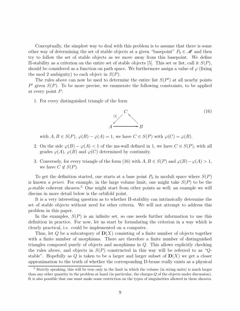
The rules above can now be used to determine the entire list S(P ′) at all nearby pointsP ′ given S(P ). To be more precise, we enumerate the following constraints, to be appliedat every point P :

1. For every distinguished triangle of the form

C[1]

~~~~

~~~

A // B

__@@@@@@@

(16)

with A,B ∈ S(P ), ϕ(B)− ϕ(A) = 1, we have C ∈ S(P ) with ϕ(C) = ϕ(B).

2. On the side ϕ(B)− ϕ(A) < 1 of the ms-wall defined in 1, we have C ∈ S(P ), with allgrades ϕ(A), ϕ(B) and ϕ(C) determined by continuity.

3. Conversely, for every triangle of the form (16) with A,B ∈ S(P ) and ϕ(B)−ϕ(A) > 1,we have C 6∈ S(P ).

To get the definition started, one starts at a base point P0 in moduli space where S(P )is known a priori. For example, in the large volume limit, one might take S(P ) to be theµ-stable coherent sheaves.5 One might start from other points as well; an example we willdiscuss in more detail below is the orbifold point.

It is a very interesting question as to whether Π-stability can intrinsically determine theset of stable objects without need for other criteria. We will not attempt to address thisproblem in this paper.

In the examples, S(P ) is an infinite set, so one needs further information to use thisdefinition in practice. For now, let us start by formulating the criterion in a way which isclearly practical, i.e. could be implemented on a computer.

Thus, let Q be a subcategory of D(X) consisting of a finite number of objects togetherwith a finite number of morphisms. There are therefore a finite number of distinguishedtriangles composed purely of objects and morphisms in Q. This allows explicitly checkingthe rules above, and objects in S(P ) constructed in this way will be referred to as “Q-stable”. Hopefully as Q is taken to be a larger and larger subset of D(X) we get a closerapproximation to the truth of whether the corresponding D-brane really exists as a physical

5 Strictly speaking, this will be true only in the limit in which the volume (in string units) is much largerthan any other quantity in the problem at hand (in particular, the chargesQ of the objects under discussion).It is also possible that one must make some restriction on the types of singularities allowed in these sheaves.

9

object. There are probably many mathematical subtleties which need to be overcome tomake this hope more manifest.

The first criticism one can make of this proposal is that stability, which should be aphysical notion, depends on position in the path space P rather than the moduli spaceitself. As we explore in section 4, the physical identity of an object in D(X) undergoesmonodromy on going around singularities in M and so one cannot expect the notion ofstability of an object in D(X) to depend only on the position in M . However, one shouldexpect stability to be a function of position in the Teichmuller space T . That is, a loop inM not enclosing anything like a conifold point, Gepner point, etc., should be trivial and sothe notion of stability should not change upon monodromy around this loop.

As we commented earlier, the value of ϕ for objects with general charge will be ambiguouson T . However, our rules for stability only use the ϕ’s of stable objects; indeed there is noclear physical definition of ϕ for an unstable object.

Grades of stable objects will be unambiguous on T if no path in R(A) ⊂ T , the region inwhich A is stable, encloses a zero Z(A;P ) = 0. This will be true if we grant two conditions.First, stable objects cannot become massless at non-singular points in moduli space,

Z(A;P ) 6= 0 ∀A ∈ S(P ). (17)

Of course this is also a physical consistency condition — such a massless state would haveshown up as a singularity of the conformal field theory and in the conjugate period. Second,we will assume that R(A) is simply connected.6

In the finite approximation of Q-stability, a massless object in Q which is Q-stable at asmooth point in M should become Q-unstable if we increase the size of Q to more closelyapproximate real physics. We therefore define a collection Q to be “s-complete” if no Q-stable objects become massless at a (smooth) point in M .

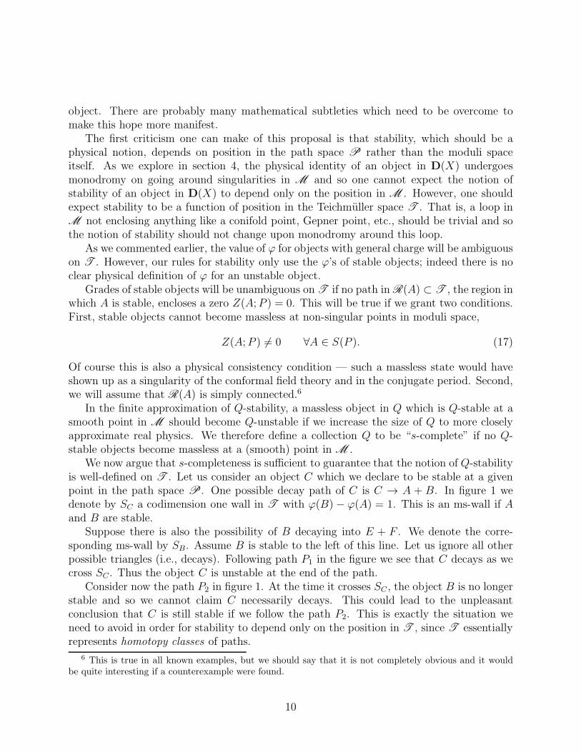
We now argue that s-completeness is sufficient to guarantee that the notion of Q-stabilityis well-defined on T . Let us consider an object C which we declare to be stable at a givenpoint in the path space P. One possible decay path of C is C → A + B. In figure 1 wedenote by SC a codimension one wall in T with ϕ(B)− ϕ(A) = 1. This is an ms-wall if Aand B are stable.

Suppose there is also the possibility of B decaying into E + F . We denote the corre-sponding ms-wall by SB. Assume B is stable to the left of this line. Let us ignore all otherpossible triangles (i.e., decays). Following path P1 in the figure we see that C decays as wecross SC . Thus the object C is unstable at the end of the path.

Consider now the path P2 in figure 1. At the time it crosses SC , the object B is no longerstable and so we cannot claim C necessarily decays. This could lead to the unpleasantconclusion that C is still stable if we follow the path P2. This is exactly the situation weneed to avoid in order for stability to depend only on the position in T , since T essentiallyrepresents homotopy classes of paths.

6 This is true in all known examples, but we should say that it is not completely obvious and it wouldbe quite interesting if a counterexample were found.

10

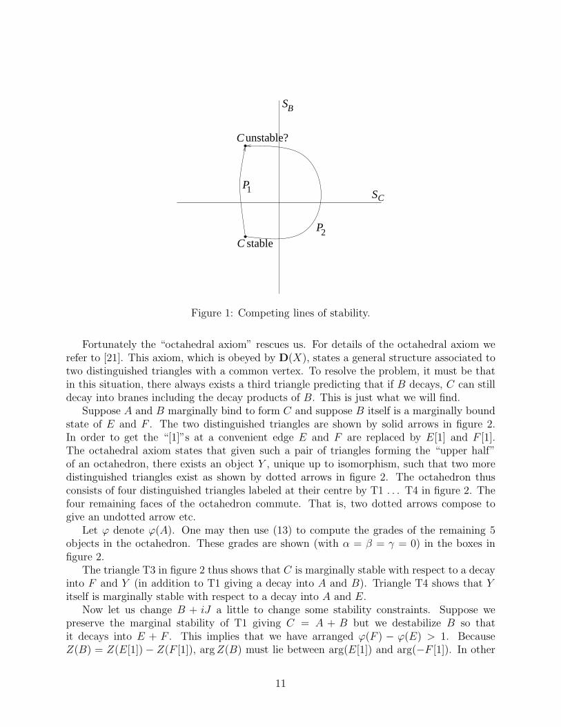
stable

P

S

S

unstable?

P

C

C

B

2

1C

Figure 1: Competing lines of stability.

Fortunately the “octahedral axiom” rescues us. For details of the octahedral axiom werefer to [21]. This axiom, which is obeyed by D(X), states a general structure associated totwo distinguished triangles with a common vertex. To resolve the problem, it must be thatin this situation, there always exists a third triangle predicting that if B decays, C can stilldecay into branes including the decay products of B. This is just what we will find.

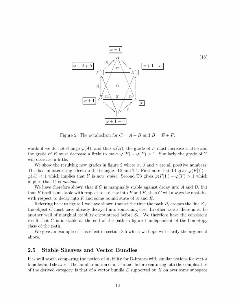
Suppose A and B marginally bind to form C and suppose B itself is a marginally boundstate of E and F . The two distinguished triangles are shown by solid arrows in figure 2.In order to get the “[1]”s at a convenient edge E and F are replaced by E[1] and F [1].The octahedral axiom states that given such a pair of triangles forming the “upper half”of an octahedron, there exists an object Y , unique up to isomorphism, such that two moredistinguished triangles exist as shown by dotted arrows in figure 2. The octahedron thusconsists of four distinguished triangles labeled at their centre by T1 . . . T4 in figure 2. Thefour remaining faces of the octahedron commute. That is, two dotted arrows compose togive an undotted arrow etc.

Let ϕ denote ϕ(A). One may then use (13) to compute the grades of the remaining 5objects in the octahedron. These grades are shown (with α = β = γ = 0) in the boxes infigure 2.

The triangle T3 in figure 2 thus shows that C is marginally stable with respect to a decayinto F and Y (in addition to T1 giving a decay into A and B). Triangle T4 shows that Yitself is marginally stable with respect to a decay into A and E.

Now let us change B + iJ a little to change some stability constraints. Suppose wepreserve the marginal stability of T1 giving C = A + B but we destabilize B so thatit decays into E + F . This implies that we have arranged ϕ(F ) − ϕ(E) > 1. BecauseZ(B) = Z(E[1])− Z(F [1]), argZ(B) must lie between arg(E[1]) and arg(−F [1]). In other

11

B

!!CCCC

CCCC

F [1]

[1]

[1]==

E[1]oo

C[1] //

""

A

VV,,,,,,,,,,,,,,,,,,,,,

OO

Y[1]

<<

VV

ϕ

ϕ+ 1− α

ϕ+ 1− γ

ϕ+ 1

ϕ+ 2 + β

ϕ+ 1

T1

T2

T3 T4

(18)

Figure 2: The octahedron for C = A+B and B = E + F .

words if we do not change ϕ(A), and thus ϕ(B), the grade of F must increase a little andthe grade of E must decrease a little to make ϕ(F ) − ϕ(E) > 1. Similarly the grade of Ywill decrease a little.

We show the resulting new grades in figure 2 where α, β and γ are all positive numbers.This has an interesting effect on the triangles T3 and T4. First note that T4 gives ϕ(E[1])−ϕ(A) < 1 which implies that Y is now stable. Second T3 gives ϕ(F [1]) − ϕ(Y ) > 1 whichimplies that C is unstable.

We have therefore shown that if C is marginally stable against decay into A and B, butthat B itself is unstable with respect to a decay into E and F , then C will always be unstablewith respect to decay into F and some bound state of A and E.

Referring back to figure 1 we have shown that at the time the path P2 crosses the line SC ,the object C must have already decayed into something else. In other words there must beanother wall of marginal stability encountered before SC . We therefore have the consistentresult that C is unstable at the end of the path in figure 1 independent of the homotopyclass of the path.

We give an example of this effect in section 3.5 which we hope will clarify the argumentabove.

2.5 Stable Sheaves and Vector Bundles

It is well worth comparing the notion of stability for D-branes with similar notions for vectorbundles and sheaves. The familiar notion of a D-brane, before venturing into the complexitiesof the derived category, is that of a vector bundle E supported on X on over some subspace

12

of X . The connection on this bundle must satisfy the Hermitian-Yang-Mills equation.A bundle E has a “slope” µ given by

µ(E) =1

rank(E)

∫

c1(E) ∧ (∗J) (19)

where J is the Kahler form. A bundle E is said to be stable if it is associated to a sheaf E

such that every coherent subsheaf F of lower rank satisfies µ(F ) < µ(E ). It is semistable

if the weaker condition µ(F ) ≤ µ(E ) holds.We then have the following theorem due to Donaldson, Uhlenbeck and Yau [25, 26]

Theorem 1 An bundle is stable if and only if it admits an irreducible Hermitian-Yang-Mills

connection. This connection is unique.

As shown in [9] this stability condition is implied by Π-stability at large radius limit aswe now review. Suppose F is a subsheaf of E . We then have a short exact sequence

0 → F → E → G → 0, (20)

for some G which yields a distinguished triangle in the derived category in the usual way.Near the large radius limit we may use (9) to show

ϕ(E ) ≈ −1

πtan−1 2V

µ(E ), (21)

where V is the volume of X . The stability condition µ(F ) < µ(E ) is then equivalent toϕ(F ) < ϕ(E ). Since ch(E ) = ch(F ) + ch(G ), we have Z(E ) = Z(F ) + Z(G ) and so ϕ(E )lies between ϕ(F ) and ϕ(G ). It follows that µ(F ) < µ(E ) implies that ϕ(F )−ϕ(G [−1]) < 1and so E = Cone(G [−1] → F ) is Π-stable with respect to the triangle associated to (20).

Comparing this with the earlier discussion of Π-stability, the main point of difference isthat the coherent sheaves form an abelian category: one has a well-defined notion of kernelsand cokernels. The statement that “F is a subsheaf of E ” is another way of saying that themorphism F → E has no kernel and so the statement depends on the abelian structure ofthe category.

The derived category of coherent sheaves is not an abelian category and hence has noabsolute notion of “sub-D-brane”. In checking the stability of a sheaf one has to check forstability only against all subsheaves. Since a subsheaf has a lower rank, this is always afinite process. For D-branes however there is no such hierarchy of objects such as rank andtherefore no analogue of a finite chain of possible decay products. Given two D-branes Aand B, it is known in examples that A can decay into B for some values of the Kahler form,while B can decay into A for other values, as we will see in subsection 4.1. It is this lackof hierarchy between D-branes and their decay products which forces one to use a categorywhich is not abelian, rather than simpler notions such as sheaves.

13

2.6 Abelian subcategories and the orbifold point

The arguments we just made do not yet rule out the possibility that in specific regions ofTeichmuller space, one can reduce the general discussion of Π-stability to stability in anabelian category, as proposed in [9]. Thus, let us explore the claim that in some regionR, the Π-stable objects are precisely those objects E which satisfy ϕ(E ′) < ϕ(E) for allsubobjects E ′ of E defined with respect to an abelian category AR.

It is convenient to impose the further requirement that AR is a graded abelian categorywith integer gradings (as usual).

At present, the only known case of a point at which all relative gradings are integer,ϕ(E) − ϕ(F ) ∈ Z, is the orbifold point (for a C

3/Γ orbifold singularity). Near such anorbifold point, we can use conventional N = 1 supersymmetric gauge theory to describe allbound states of fractional branes, as has been observed in many works. We now give physicalarguments why this is so, to better understand in what situations this simplification mighthold.

Consider a combination of fractional branes; it will fall into one of three classes. If thecentral charges of all the branes roughly align, then all tachyonic modes have small massescompared to the string scale, and the conditions for applicability of low energy world-volumefield theory are clearly met. On the other hand, if some branes have roughly anti-alignedcentral charge, we can further distinguish the cases in which a fractional brane and its ownantibrane are both present, and the case in which this is not so. In the first case, since themass of the brane-antibrane tachyon is string scale and much larger than any other scale, thelowest energy configuration clearly will condense this tachyon, leading to brane-antibraneannihilation and a configuration with a simpler description (in terms of fewer fractionalbranes). In the second case, examination of the orbifold spectrum shows that there areno brane-antibrane tachyons present, so no possibility for a bound state involving all ofthe objects. Again, the simple bound states can be described using only branes or onlyantibranes.

This last point in the argument relies on a condition on the spectrum which holds nearthe orbifold point but not necessarily for a general collection of branes. Thus the conditionthat the constituent brane central charges roughly align is necessary but not sufficient forthe applicability of supersymmetric gauge theory. The additional condition that the onlystring-scale tachyons are those between a brane and its own antibrane is sufficient; we havenot established that it is necessary.

Having justified the use of supersymmetric gauge theory in a region Rorb around theorbifold point, we note that indeed Π-stability reduces to a stability condition in an abeliancategory in this region; in fact we have justified the use of θ-stability near the orbifold pointas in [27], using the category of quiver representations.

We now ask what is the boundary of this region Rorb. The primary constraint is thatmorphisms Hom(E, F ) of negative degree can only be produced by flow from morphismsof degree zero. This is clear because we require every decay predicted by Π-stability tocorrespond to a decay into a subobject.

14

A sufficient (but perhaps not necessary) condition for this is to require that, comparedto the orbifold point,

|∆ϕ(E)−∆ϕ(F )| < 1 (22)

for all differences of gradings of objects in AR.This condition determines the region Rorb around the orbifold point in which the category

of quiver representations can be used to define stability. For C3/Z3, its boundary (within

the fundamental region) is the ms-line on which the D2-brane becomes stable. It is easilyseen that this stability condition breaks down on the boundary of this region.

Within Rorb, the appropriate notion of stability is a generalized notion of θ-stability,which uses the same definition of subobject, but in which the stability condition θ ·n > θ ·n′

for every subobject E ′ → E is replaced by the condition ϕ(E ′) < ϕ(E). The hierarchybetween branes and decay products is governed by the total number of fractional branes,which is always decreasing in subobjects; this number is determined by the charge of anobject.

For more general (compact) Calabi–Yau’s, there probably does not exist any point inmoduli space at which all brane central charges roughly align or antialign. Such pointswill exist for subcategories of branes carrying a subset of the possible charges, and it wouldprobably be quite useful to analyze the spectrum within these subcategories along the lineswhich we just described. Let us however continue to discuss proposals which could describeall the branes.

A logical extension of the considerations in this subsection is to try to find a set of regionsRi whose union covers the Teichmuller space, and corresponding graded categories Ai eachappropriate in a region Ri, meaning that within Ri all decays predicted by Π-stability infact reduce to decays into subobjects as defined within Ai. If such a picture can be madeto work, it would be reasonable to refer to the regions Ri as “phases,” as the choice of Ai

already tells us quite a lot of information about the BPS spectrum.The simplest proposal for constructing such an abelian category Ai goes as follows. First,

one needs to postulate integer gradings for all of the objects. The simplest prescription onecan make is to take the gradings ϕ(E) at a specific point P in moduli space and round themoff to the nearest integer; call this n(E). As long as we make a consistent choice of n(E) foreach E, any choice of rounding will work. This choice then leads to a definition of integergrading for each morphism; let n(f) be the grading of the morphism f .

As in the orbifold example, we want to arrange things so that all decays predicted byΠ-stability in fact proceed through subobjects as defined by exact sequences involving mor-phisms of grading n = 0. This condition will again define the region R in which a givenchoice of integer gradings can be used. A potential difficulty with this idea appears at thispoint, as there is no guarantee that the region R so defined will have finite extent.

Assuming it does, one then wants to show that this data indeed defines an abeliancategory; in particular that morphisms have kernels and cokernels. As mentioned in [5], theappropriate framework for this discussion is the formalism of t-structures; we hope to returnto this in future work.

15

3 Examples on the Quintic

The analysis of section 2 is clarified in this section by analyzing various examples of Π-stability in the context of the quintic hypersurface in P4.

3.1 Basics of the moduli space and periods

In this section we review the techniques required from Candelas et al [1]. Let X be thequintic hypersurface in P4. The mirror Y is then a (Z5)

3 orbifold of a quintic with generaldefining equation

x50 + x51 + x52 + x53 + x54 − 5ψx0x1x2x3x4. (23)

The single complex variable ψ spans the one-dimensional moduli space of complex structuresof Y . This encodes the mirror of the one-dimensional moduli space of complexified Kahlerforms on X . It is useful to introduce the variable z = (5ψ)−5.

The Gepner point of the moduli space of X is mirror to ψ = 0. The large radius limitof X is mirror to z = 0. At ψ = 1, one has the “conifold” point where Y becomes singular(acquiring a conifold point). This is mirror to the fact that the conformal field theory on Xbecomes singular for the corresponding value of B + iJ .

Since dimH3(Y ) = 4, we have 4 independent periods∫

ΓΩ for the holomorphic 3-form

Ω. These periods satisfy the Picard-Fuchs equation (see [28] for a nice account of this).Following [1] we use the following periods given as a power series around the Gepner point:

j = −15

∞∑

m=1

α(2+j)mΓ(m5)

Γ(m)Γ(1− m5)4z−

m

5 . (24)

We may use 0, . . . , 3 as a basis.7

One may then analytically continue these periods using Barnes’ integral methods tomatch this basis with series around the large radius limit. We use the following basis nearz = 0:

Φ0 =1

2πi

∫

Γ(5s+ 1)Γ(−s)Γ(s+ 1)4

(eπiz)s ds

=∞∑

n=0

(5n)!

n!5zn

= −15

∞∑

m=1

α2mΓ(m5)

Γ(m)Γ(1− m5)4z−

m

5

= 0.

(25)

7 In this section and section 4, we follow the convention that the relation (10) between ϕ(E) and Z(E)has an additional minus sign, and Z(E) is the complex conjugate of that defined in (9).

16

Φ1 = − 1

2πi· 1

2πi

∫

Γ(5s+ 1)Γ(−s)2Γ(s+ 1)3

zs ds

=1

2πilog z +O(z) = t+O(e2πit)

= −15(0 − 31 − 22 −3).

(26)

Φ2 = − 1

2π2· 1

2πi

∫

Γ(5s+ 1)Γ(−s)3Γ(s+ 1)2

(eπiz)s ds

= − 1

4π2(log z)2 +

1

2πilog z − 5

6+O(z)

= t2 + t− 56+O(e2πit)

= 25(−20 +2 +3).

(27)

Φ3 =1

(2πi)3· (−6) · 1

2πi

∫

Γ(5s+ 1)Γ(−s)4Γ(s+ 1)

zs ds

=i

8π3(log z)3 +

7i

4πlog z − 30iζ(3)

π3+O(z)

= t3 − 72t− 30iζ(3)

π3+O(e2πit)

= −65(21 + 22 +3).

(28)

These analytic continuations are valid for

−2π < arg z < 0. (29)

In each case above the integral is taken along the path corresponding to a straight linefrom s = ǫ − i∞ to s = ǫ + i∞, where 0 < ǫ < 1. The variable t above corresponds toB + iJ = te1 for X where e1 generates H2(X,Z). The “mirror map” determines t uniquelyas

t =Φ1

Φ0. (30)

We refer to [29], for example, for an account of the history and status of the mirror map.The above results show that the true stringy complexified Kahler moduli space M of X

is the P1 with affine coordinate z; the periods are singular or have branch points at the threepoints mentioned above. (The Gepner point is only an orbifold singularity, and physics isnonsingular there.)

As discussed in section 2.4 the stability questions are best thought of in terms of theTeichmuller space rather than the moduli space. In terms of the “presentation of data”we wish to give in this example, we basically have three choices of how to parametrize theKahler moduli space:

17

1. We can use z (or ψ) as above as a parameter on the moduli space. Since z is not aparameter on the Teichmuller space, the periods and questions of stability will not bea single valued function of z.

2. We can use the theory of automorphic functions to construct the Teichmuller spaceas the upper half-plane as was done in section 2.2 of [1]. This has the advantage ofpresenting the periods as single valued functions. The disadvantage of this approachis that this Teichmuller space appears to be remarkably unphysical. For example, thereal line of the upper half-plane will contain a dense set of copies of both the conifoldpoint and the large radius limit point. The former are a finite distance from a genericpoint in the moduli space while the latter are an infinite distance! This is tied in withproblems of notions of T-duality for such string compactifications [30].

3. We can use t = B + iJ as the parameter. This is the most physical parameter for themoduli space. The disadvantage of this approach is that fundamental regions of themoduli space do not “tile” the t-plane leading to multivaluedness as in the z-plane.This problem should be clear from the figures in section 3.

The choice we make in this paper is to go with the third option and use t to plot lines ofmarginal stability. This is viable because the lines of marginal stability we consider usuallyremain in the “Calabi–Yau” phase, i.e., remain on the large radius side of the conifold point.In this phase, t is certainly the most natural parameter. Some of the ms-lines analyzedlater in this section venture outside this phase but they do not do unpleasant things such ascrossing themselves when plotted in the t-plane. If such pathologies occur, as they surely doin more complicated examples, it might be easier to visualize the ms-lines in the less physicalchoice of using the upper half-plane as the Teichmuller space.

3.2 The exact computation of ϕ

For a Calabi–Yau threefold, an A-type D-brane corresponds to a 3-cycle. The central charge,Z, of this D-brane is then given, up to some normalization, exactly by the period associatedto this cycle. The normalization will not concern us since we are only interested in differencesin gradings and hence ratios of periods. We may use this fact, together with the knowledge ofsection 3.1, to determine the exact central charges of B-type branes on the quintic threefold.

Given a particular element of D(X) we may compute the Chern character using

ch(E •) =∑

n

(−1)n ch(E n). (31)

Equation (9) then determines the large radius behaviour of Z(E •) as a series in t. This isthen enough to fix the exact linear combination of j’s from section 3.1 which representsthe period on Y and hence the exact form of Z(E •).

In order to perform this analysis we need to know precisely what constitutes the “quantumcorrections” of (9). These corrections come from two sources:

18

1. Nonperturbative corrections: These are of the form an exp(2πint) for n > 0.

2. Perturbative corrections: These are of the form bmtm. Since these corrections begin at

“four loops” [31], the highest power of t appearing will be three less than the leadingorder (“one loop”) term.

Note therefore that the only effect of the perturbative corrections is to contribute a constantterm in (28). We claim that this constant term acts to cancel the 30iζ(3)/π3 term in (28).One way to justify this is to do a direct computation of the 4-loop term which we have notdone.

Instead let us use the fact the the singularity in the conformal field theory associate toX at the “conifold point” is associated to a D-brane becoming massless. The monodromy ofthe periods around the conifold point given by table 3.1 of [1] immediately implies that theperiod associated to this D-brane must be −0 + 1. The analysis of the previous sectionshows that at large radius this period behaves as

56t3 + 25

12t− 25iζ(3)

π3. (32)

Using (9) and td(TX) = 1 + 56e21 for the quintic we have

ch(E •) = 1 +

(

c− 25iζ(3)

π3

)

e31, (33)

where c represents the 4-loop correction. Since c is imaginary (see [1] for example) the realityof ch confirms our assertion.

Furthermore we see immediately that the D-brane that vanishes at the conifold pointsatisfies ch(E •) = 1. It is therefore natural to associate it with the structure sheaf O asasserted in [32].

Now that we have fixed this 4-loop term we have an exact method for associating a linearcombination of j’s (over the rational numbers) with the central charge of any element ofD(X). We therefore have an exact method of computing the grade ϕ of any B-type D-brane on the quintic. This method should generalize to any example where the Picard-Fuchssystem is understood in the language of generalized hypergeometric functions.

In the examples below we computed ϕ numerically by integrating the Picard–Fuchs equa-tion with a Runge–Kutta algorithm. The initial conditions were specified by using the powerseries expansions of j (24).

3.3 N D4-branes

As a first example consider the following map

O(−N)f(xi) //O , (34)

19

0

1

2

3

4

5

6

-1 0 1 2 3 4 5 6 7

"N=1""N=2""N=3""N=4""N=5""N=6"

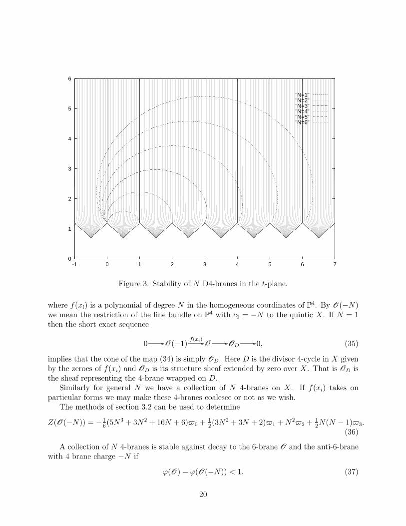
Figure 3: Stability of N D4-branes in the t-plane.

where f(xi) is a polynomial of degree N in the homogeneous coordinates of P4. By O(−N)we mean the restriction of the line bundle on P4 with c1 = −N to the quintic X . If N = 1then the short exact sequence

0 //O(−1)f(xi) //O //OD

//0, (35)

implies that the cone of the map (34) is simply OD. Here D is the divisor 4-cycle in X givenby the zeroes of f(xi) and OD is its structure sheaf extended by zero over X . That is OD isthe sheaf representing the 4-brane wrapped on D.

Similarly for general N we have a collection of N 4-branes on X . If f(xi) takes onparticular forms we may make these 4-branes coalesce or not as we wish.

The methods of section 3.2 can be used to determine

Z(O(−N)) = −16(5N3 + 3N2 + 16N + 6)0 +

12(3N2 + 3N + 2)1 +N22 +

12N(N − 1)3.

(36)

A collection of N 4-branes is stable against decay to the 6-brane O and the anti-6-branewith 4 brane charge −N if

ϕ(O)− ϕ(O(−N)) < 1. (37)

20

The resulting lines of marginal stability for various values of N are shown in figure 3. TheD4 branes are stable above the line (i.e., large radius) as one would expect. Note that thispicture is of a series of fundamental regions in the t-plane each spanning a shift in the B-field (i.e., real part of t) by one. The starting region, as required by (29), is the one where−1 < B < 0. The regions to the right are obtained by analytic continuation.

Note that the lines of marginal stability have one end at the conifold point where Z(O)vanishes and the other end is at the copy of the conifold point where Z(O(−N)) vanishes.This is a general feature of the lines of marginal stability. They can only end at a pointwhere arg(Z) becomes ill-defined, i.e., where one of the periods vanishes.

Note that for large N one may use (9) directly to show that asymptotically the line ofstability becomes an arc of a circle of radius N/

√3 with centre t = N/2 + iN/2

√3.

3.4 Some exotic D-branes

As discussed in [10] one may use the D4-brane construction in section 3.3 as a basis of a con-struction of more exotic objects. The map f(xi) in (34) lives in the space Hom(O(−N),O) =Hom(O ,O(N)) = Ext0(O ,O(N)) = H0(O(N)) (see, for example, [33]). By Serre duality,H0(O(N)) is dual to H3(O(−N)) = Ext3(O ,O(−N)). Thus every example of a map f hassome “dual” map f∨ ∈ Ext3(O ,O(−N)).

In terms of the derived category, an element of Ext3(O ,O(−N)) is a morphism

Of∨

//O(−N)[3], (38)

where, recalling the notation of section 2.1, O(−N)[3] refers to a complex whose only nontriv-ial entry is O(−N) at position −3. The cone of this map XN = Cone(f∨ : O → O(−N)[3])is an object in D(X) we wish to study in this section. Note that we may deform XN into awhole family of D-branes by varying f∨ — just as 4-branes may be deformed by varying f .

The rules of section 2 require that ϕ(E [n]) = ϕ(E ) + n. It follows that the condition forstability of XN is that

3 + ϕ(O(−N))− ϕ(O) < 1. (39)

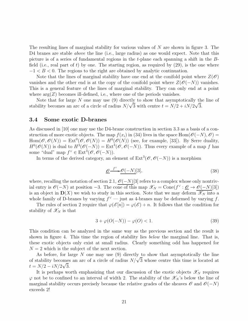
This condition can be analyzed in the same way as the previous section and the result isshown in figure 4. This time the region of stability lies below the marginal line. That is,these exotic objects only exist at small radius. Clearly something odd has happened forN = 2 which is the subject of the next section.

As before, for large N one may use (9) directly to show that asymptotically the lineof stability becomes an arc of a circle of radius N/

√3 whose centre this time is located at

t = N/2 − iN/2√3.

It is perhaps worth emphasizing that our discussion of the exotic objects XN requiresϕ not be to confined to an interval of width 2. The stability of the XN ’s below the line ofmarginal stability occurs precisely because the relative grades of the sheaves O and O(−N)exceeds 2!

21

0

0.5

1

1.5

2

2.5

3

-1 0 1 2 3 4 5 6 7

"N=1""N=2""N=3""N=4""N=5""N=6"

Figure 4: Stability of the exotic objects XN in the t-plane.

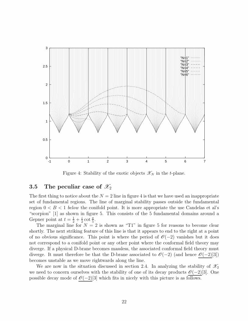
3.5 The peculiar case of X2

The first thing to notice about theN = 2 line in figure 4 is that we have used an inappropriateset of fundamental regions. The line of marginal stability passes outside the fundamentalregion 0 < B < 1 below the conifold point. It is more appropriate the use Candelas et al’s“scorpion” [1] as shown in figure 5. This consists of the 5 fundamental domains around aGepner point at t = 1

2+ i

2cot π

5.

The marginal line for N = 2 is shown as “T1” in figure 5 for reasons to become clearshortly. The next striking feature of this line is that it appears to end to the right at a pointof no obvious significance. This point is where the period of O(−2) vanishes but it doesnot correspond to a conifold point or any other point where the conformal field theory maydiverge. If a physical D-brane becomes massless, the associated conformal field theory mustdiverge. It must therefore be that the D-brane associated to O(−2) (and hence O(−2)[3])becomes unstable as we move rightwards along the line.

We are now in the situation discussed in section 2.4. In analyzing the stability of X2

we need to concern ourselves with the stability of one of its decay products O(−2)[3]. Onepossible decay mode of O(−2)[3] which fits in nicely with this picture is as follows.

22

0

0.5

1

1.5

2

-1 -0.5 0 0.5 1 1.5 2

"T1""T2""T3""T4"

Figure 5: Lines of stability for the case of X2.

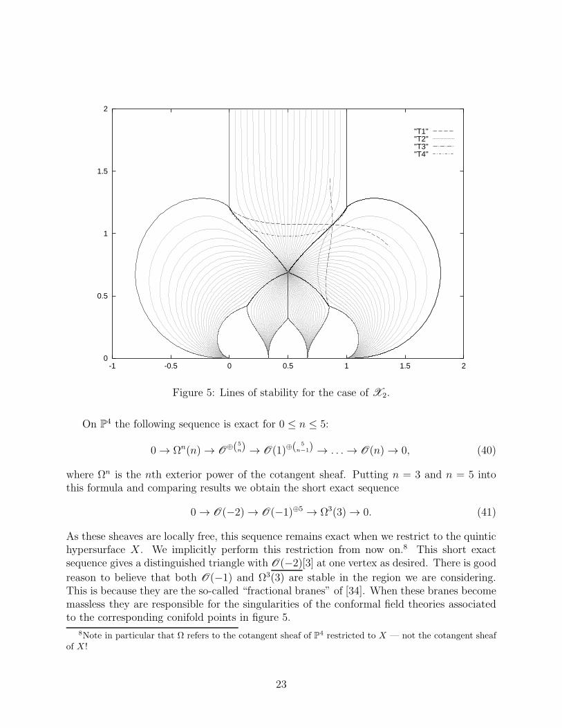
On P4 the following sequence is exact for 0 ≤ n ≤ 5:

0 → Ωn(n) → O⊕(5n) → O(1)⊕(

5

n−1) → . . .→ O(n) → 0, (40)

where Ωn is the nth exterior power of the cotangent sheaf. Putting n = 3 and n = 5 intothis formula and comparing results we obtain the short exact sequence

0 → O(−2) → O(−1)⊕5 → Ω3(3) → 0. (41)

As these sheaves are locally free, this sequence remains exact when we restrict to the quintichypersurface X . We implicitly perform this restriction from now on.8 This short exactsequence gives a distinguished triangle with O(−2)[3] at one vertex as desired. There is good

reason to believe that both O(−1) and Ω3(3) are stable in the region we are considering.This is because they are the so-called “fractional branes” of [34]. When these branes becomemassless they are responsible for the singularities of the conformal field theories associatedto the corresponding conifold points in figure 5.

8Note in particular that Ω refers to the cotangent sheaf of P4 restricted to X — not the cotangent sheafof X !

23

O(−2)[3]

&&NNNNNNNNNNN

Ω3(3)[3]

[1]

[1]88qqqqqqqqqq

O(−1)5[3]oo

X2

[1] //

&&

O

ZZ555555555555555555555555

OO

Y

[1]

77

ZZ

T1

T2

T3 T4

(42)

Figure 6: The octahedron for X2.

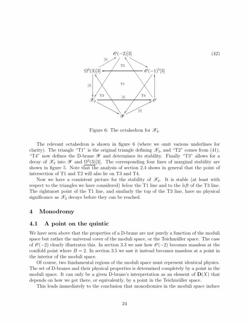
The relevant octahedron is shown in figure 6 (where we omit various underlines forclarity). The triangle “T1” is the original triangle defining X2, and “T2” comes from (41).“T4” now defines the D-brane Y and determines its stability. Finally “T3” allows for adecay of X2 into Y and Ω3(3)[3]. The corresponding four lines of marginal stability areshown in figure 5. Note that the analysis of section 2.4 shows in general that the point ofintersection of T1 and T2 will also lie on T3 and T4.

Now we have a consistent picture for the stability of X2. It is stable (at least withrespect to the triangles we have considered) below the T1 line and to the left of the T3 line.The rightmost point of the T1 line, and similarly the top of the T3 line, have no physicalsignificance as X2 decays before they can be reached.

4 Monodromy

4.1 A point on the quintic

We have seen above that the properties of a D-brane are not purely a function of the modulispace but rather the universal cover of the moduli space, or the Teichmuller space. The caseof O(−2) clearly illustrates this. In section 3.3 we saw how O(−2) becomes massless at theconifold point where B = 2. In section 3.5 we saw it instead becomes massless at a point inthe interior of the moduli space.

Of course, two fundamental regions of the moduli space must represent identical physics.The set of D-branes and their physical properties is determined completely by a point in themoduli space. It can only be a given D-brane’s interpretation as an element of D(X) thatdepends on how we got there, or equivalently, by a point in the Teichmuller space.

This leads immediately to the conclusion that monodromies in the moduli space induce

24

autoequivalences of D(X). Such an autoequivalence is always induced by a Fourier–Mukaitransform [35]. Fixing notation, given projections

X ×Xp1

vvvvvv

vvv

p2

##HHHHHH

HHH

X X

(43)

an object Ψ ∈ D(X ×X) induces a transform

TΨ(A) = Rp2∗(ΨL

⊗ p∗1A), (44)

for any object A of D(X).Based on the action on the Chern characters, Kontsevich [36] conjectured that for the

monodromy around the conifold point in the case of the quintic, Ψ is given by

. . .→ 0 → OX×X → O∆ → 0 → . . . , (45)

where ∆ ⊂ X × X is the diagonal embedding of X , and the map in (45) is the obviousrestriction map. Seidel and Thomas [37] analyzed many aspects of this transform in thecontext of “homological mirror symmetry”. Indeed they outlined an interesting frameworkin this context in which one can motivate Kontsevich’s conjecture. (Note that we will notdirectly appeal to this conjectured strong form of mirror symmetry in this paper.)

Note that (44) can be written in a simpler form involving only D(X):

TΨ(A) = Cone(e : Hom(O , A)⊗ O → A), (46)

where e is the evaluation map. We refer to [37] for the precise definitions of the manipulationsin (46).

We are now in a position to justify Kontsevich’s proposal at the level of the derivedcategory, rather than just the cohomology class of Chern characters. We begin with the0-brane A = Op, i.e., the skyscraper sheaf at a point p ∈ X at zeroth position in thecomplex.

Let Ip denote the ideal sheaf of functions vanishing at p. The short exact sequence

0 → Ip → O → Op → 0, (47)

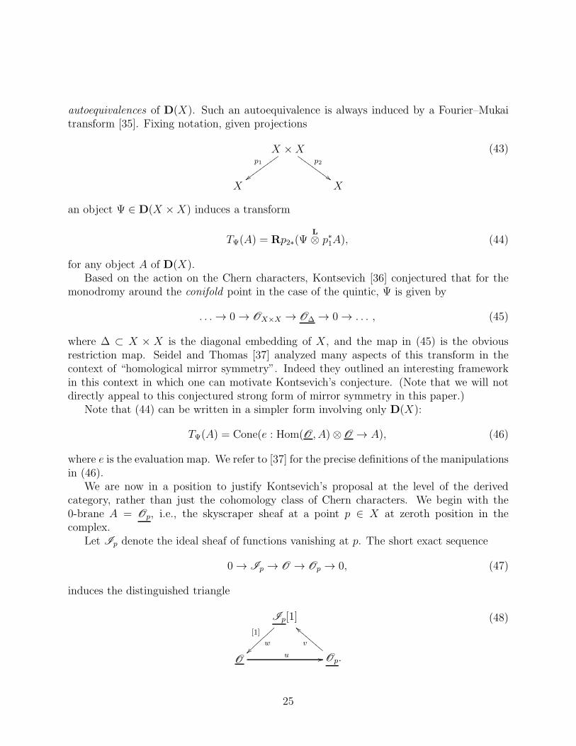
induces the distinguished triangle

Ip[1]

w

[1]

~~||||

||||

Ou // Op.

v

aaDDDDDDDD

(48)

25

-3

-2

-1

0

1

2

3

0 0.5 1 1.5 2

"ideal""point"

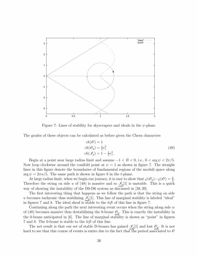
Figure 7: Lines of stability for skyscrapers and ideals in the ψ-plane.

The grades of these objects can be calculated as before given the Chern characters

ch(O) = 1

ch(Op) =15e31

ch(Ip) = 1− 15e31.

(49)

Begin at a point near large radius limit and assume −1 < B < 0, i.e., 0 < argψ < 2π/5.Now loop clockwise around the conifold point at ψ = 1 as shown in figure 7. The straightlines in this figure denote the boundaries of fundamental regions of the moduli space alongargψ = 2πn/5. The same path is shown in figure 8 in the t-plane.

At large radius limit, when we begin our journey, it is easy to show that ϕ(Op)−ϕ(O) = 32.

Therefore the string on side u of (48) is massive and so Ip[1] is unstable. This is a quick

way of showing the instability of the D0-D6 system as discussed in [38, 39].The first interesting thing that happens as we follow the path is that the string on side

u becomes tachyonic thus stabilizing Ip[1]. This line of marginal stability is labeled “ideal”in figures 7 and 8. The ideal sheaf is stable to the left of this line in figure 7.

Continuing along the path the next interesting event occurs when the string along side wof (48) becomes massive thus destabilizing the 0-brane Op. This is exactly the instability in

the 0-brane anticipated in [6]. The line of marginal stability is shown as “point” in figures7 and 8. The 0-brane is stable to the left of this line.

The net result is that our set of stable D-branes has gained Ip[1] and lost Op. It is nothard to see that this course of events is entire due to the fact that the period associated to O

26

0

0.5

1

1.5

2

-1 -0.5 0 0.5 1 1.5 2

"ideal""point"

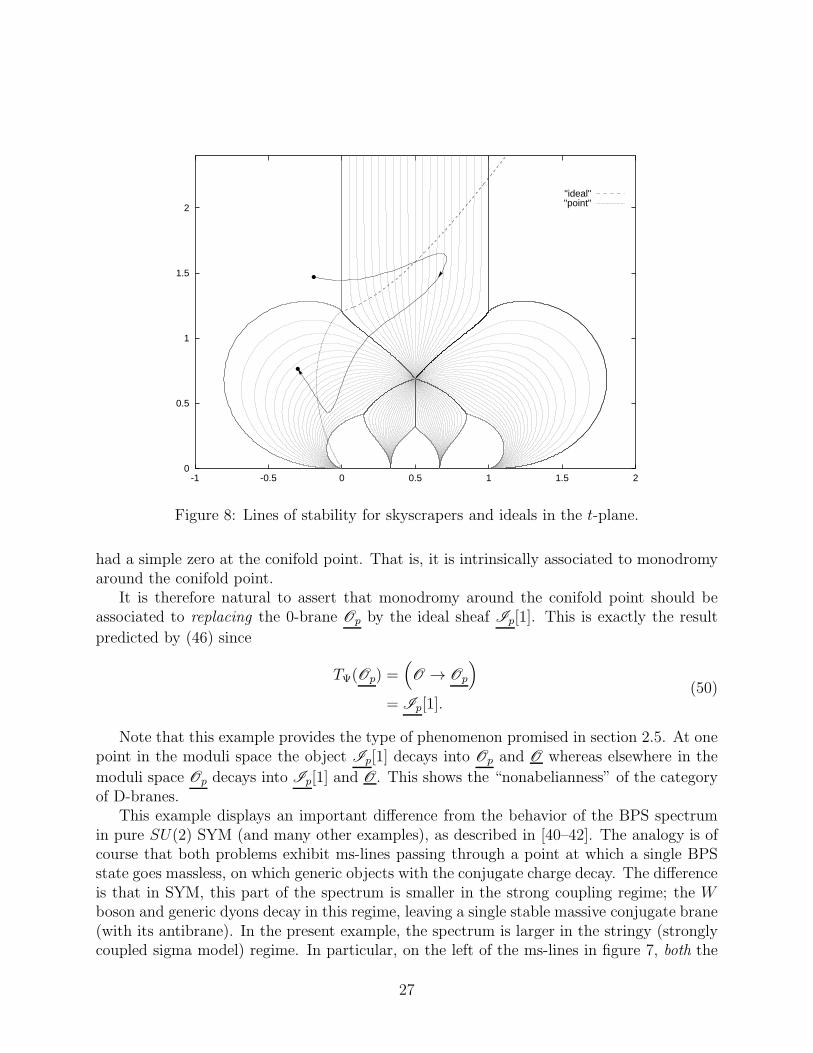
Figure 8: Lines of stability for skyscrapers and ideals in the t-plane.

had a simple zero at the conifold point. That is, it is intrinsically associated to monodromyaround the conifold point.

It is therefore natural to assert that monodromy around the conifold point should beassociated to replacing the 0-brane Op by the ideal sheaf Ip[1]. This is exactly the result

predicted by (46) since

TΨ(Op) =(

O → Op

)

= Ip[1].(50)

Note that this example provides the type of phenomenon promised in section 2.5. At onepoint in the moduli space the object Ip[1] decays into Op and O whereas elsewhere in the

moduli space Op decays into Ip[1] and O. This shows the “nonabelianness” of the categoryof D-branes.

This example displays an important difference from the behavior of the BPS spectrumin pure SU(2) SYM (and many other examples), as described in [40–42]. The analogy is ofcourse that both problems exhibit ms-lines passing through a point at which a single BPSstate goes massless, on which generic objects with the conjugate charge decay. The differenceis that in SYM, this part of the spectrum is smaller in the strong coupling regime; the Wboson and generic dyons decay in this regime, leaving a single stable massive conjugate brane(with its antibrane). In the present example, the spectrum is larger in the stringy (stronglycoupled sigma model) regime. In particular, on the left of the ms-lines in figure 7, both the

27

original D0 Op and its monodromy image Ip[1] are stable. This is a simple consequenceof the different behaviors of the central charges in the two problems, but shows that overlysimple generalizations about the qualitative behavior of the spectrum can fail.

This example is also interesting from the point of view of “D-geometry” as discussedin [43]. One of the prototypical problems one can study to get a handle on stringy geometryis the moduli space metric of the D0-brane; this D0-metric is a canonically defined metricwhich for Calabi–Yau exhibits the well-known corrections to Ricci-flatness [31], assumingthat the D0 exists in the stringy regime. What we have found is that the D0 not only(almost certainly) exists,9 but that in the stringy regime there are two candidate D0’s,which can be obtained by going around either side of the conifold point, leading to twoD0-metrics. It would be interesting to know if these are necessarily the same or are relatedin some simple way.

4.2 The general case

Given the above example we can try to generalize to the case of any object in D(X) for thequintic threefoldX . We know that the monodromy must induce an autoequivalence onD(X)and must therefore arise as a Fourier–Mukai transform associated to some Ψ ∈ D(X ×X).

Putting A = Op in (44) yields

TΨ(Op) = Rp2∗ (Ψ|p×X)

= Ψ|p×X ,(51)

where |p×X is the derived category version of the restriction map (i.e.,L

⊗ (Op ⊠ O)). Wetherefore have that

Ψ|p×X =(

O → Op

)

. (52)

The most natural and obvious solution to this equation for Ψ is that

Ψ =(

OX×X → O∆

)

(53)

as predicted by Kontsevich. We will establish this as the only possibility shortly.The argument we gave in section 4.1 generalizes directly to any object E satisfying

1 =∑

i

dimHom(O , E[i]). (54)

Given that there is a unique morphism f between O and E in some degree, there is a uniquetriangle involving these two objects and Cone(f) which will play the role of (47). Following

9 Although we did not consider decays into states with D2 or D4 charge, this is implausible for a varietyof reasons, the simplest being that such states which are known to exist have larger mass than the D0 nearthe conifold point. The stability of the 0-brane has also been anaylzed in [44].

28

the loop around the conifold point will again stabilize Cone(f) and destabilize E, againmotivating the claim that (46) is the monodromy image of E.

Note that O itself is not actually invariant upon moving around the conifold point. Onecan show that

TΨ(O) = O [−2], (55)

consistent with the claim that the combination of this FMT and flow of gradings is a physicalinvariance.

The same argument predicts that any object E with non-zero Hom(O , E[i]), not neces-sarily satisfying (54), will decay, but now one does not get a unique candidate to replace it.Besides the evaluation map e used in (46), one will in general form other objects as boundstates of E and O which are cones of other (non-canonical) maps, such as the individual ele-ments of Hom(O , E[i]) or other direct sums of these. While adiabatically varying the moduliaround the conifold point should lead to a unique decay process E → E ′ + nO , it is notcompletely clear to us that E ′ must be the monodromy image in the sense we are discussingnow; it could be that such an adiabatic process in fact changes the physical identity of thebrane.

However, by combining physical and mathematical input, one can still derive Kontsevich’sconjecture. Specifically, we need (52), the action of the monodromy on the Chern character,and the statement that the monodromy is an autoequivalence. We will appeal to a result ofBridgeland and Maciocia [45] (section 3.3), which states the following. Suppose Φ : D(Y ) →D(X) is a FMT such that for each y ∈ Y , there is a point f(y) ∈ X with

Φ(Oy) = Of(y). (56)

This induces a morphism f : Y → X and furthermore the FMT is necessarily of the form

Φ(E) = f∗(LL

⊗ E) (57)

for any E ∈ D(Y ), where L is a line bundle on Y , and f∗ is the direct image functor.By composing the true monodromy associated to the conifold point with the inverse of

the FMT (46), one obtains an autoequivalence which, under our assumptions, is an FMTthat preserves the Chern character and every point sheaf Op. This FMT is covered by theresult we just cited with f(y) = y. Using the action on the charges to determine L = OY ,we find that this composition is indeed the identity, establishing the result.

Let us turn to some related comments. It is also instructive to follow O as we go aroundthe Gepner point five times. This and its generalizations have been analyzed at the Cherncharacter level in papers such as [46–51] but not at the derived category level.

Monodromy around the large radius limit is trivially achieved by tensoring with O(1).One may then consider the combined monodromy transform given by

ΨG =(

O(1)⊠ O → O∆(1))

(58)

29

for the combined monodromy around the large radius limit and conifold point. That is, ΨG

yields monodromy around the Gepner point. One can then compute

TΨG(O) =

(

O⊕5 → O(1)

)

(TΨG)2(O) =

(

O⊕10 → O(1)⊕5 → O(2)

)

(TΨG)3(O) =

(

O⊕10 → O(1)⊕10 → O(2)⊕5 → O(3)

)

(TΨG)4(O) =

(

O⊕5 → O(1)⊕10 → O(2)⊕10 → O(3)⊕5 → O(4)

)

.

(59)

The restriction of (40) to X can then be used to show that (TΨG)4(O) = O(−1)[4]. A final

application of TΨGthen yields the result

(TΨG)5(O) = O[2]. (60)

Indeed it is an unpublished result [52] that

(TΨG)5(A) = A[2], (61)

for any A ∈ D(X). In particular “5 times around the Gepner point” is not the identity mapon D(X) but rather a shift. A similar result for the elliptic curve was described in [37].

The analysis of the quintic should extend naturally to any Calabi–Yau manifold rep-resented as a complete intersection in a toric variety. It particular, there is a “primarycomponent of the discriminant locus” in the moduli space which plays the role of the coni-fold point above as discussed by Horja [47] and Morrison [46] and also in [51]. Monodromyaround this will then also be given by the object in (45).

What about other monodromies for a general Calabi–Yau threefold? The monodromyaround the conifold point arises purely because of the simple zero appearing in Z(O). Itis clear then that the arguments above should generalize easily for any case where a singlesoliton is becoming massless at a given point in the moduli space. This is characteristic ofall “conifold”-like points as argued in [53]. We simply replace O by the particular objectS ∈ D(X) becoming massless. This yields

Ψ = Cone

(

S∨L

⊠ S → O∆

)

, (62)

as the corresponding object generating the Fourier–Mukai transform. It would be nice toestablish the more general monodromies discussed by Horja [54].

5 An Application to Supersymmetry Breaking

Let us conclude by briefly describing one possible application of these ideas, namely to findingN = 1 compactifications of string theory which spontaneously break supersymmetry.

30

In the general context of compactification with branes, a popular way to get supersymme-try breaking is to incorporate combinations of BPS space-filling branes preserving differentsupersymmetries, for example a brane and its antibrane. One could incorporate non-BPSbranes for the same purpose.

Let us discuss this type of construction in the context at hand of tree level type IIcompactification. As is well known, in this limit BPS brane considerations do not dependon the number of Minkowski dimensions filled by the branes, so we can apply Π-stability asdiscussed here to this problem, and say that a compactification will break supersymmetryin this way if the K theory class of the embedded D-branes do not support a stable orsemi-stable configuration. By semi-stable we mean a direct sum of BPS branes with alignedcentral charge, so this is just a rephrasing of the problem.

The value of this rephrasing is that, while it is not hard to find combinations of BPSbranes which break supersymmetry for a particular value of the Calabi–Yau and branemoduli, it is quite hard to find combinations which break supersymmetry for all values ofthe moduli. Indeed we are not aware of any example in the literature. Since the Calabi–Yau moduli are of course dynamical fields in the compactified theory, one must removesupersymmetric vacua at all points in moduli space to truly break supersymmetry.

To give the simplest example of what can go wrong, if one includes a brane and its ownantibrane, typically after varying moduli the two will annihilate, leaving a supersymmetricconfiguration. This is typically signaled by a tachyon in the spectrum from the start andis thus not so interesting. Many examples are known in which no tachyon is visible in thespectrum, at least for the particular Calabi–Yau moduli for which the configuration wasconstructed, and yet supersymmetry is broken. We discussed the familiar example of theD0-D6 system in section 4, and the techniques here provide many generalizations of this.

The D0-D6 configuration however does not pass the test of breaking supersymmetry forall values of the moduli; on the ms-line we exhibited in figure 7, supersymmetry is restored.This phenomenon is very generic: for example, any compactification with two types of BPSbrane would be expected to restore supersymmetry on a wall of real codimension 1. Thisalso points to the larger problem, which is that since BPS central charges vary drasticallywith the moduli, an analysis in the neighborhood of some point in moduli space is not at alladequate to address this problem. A global picture is needed.

We note in passing that a consistent string compactification with D-branes must of courseinclude orientifold planes and cancel RR tadpoles, and that one would be particularly inter-ested in finding a brane configuration of this type which breaks supersymmetry. At presentit appears that breaking supersymmetry is the hard part of the problem, while numerousexamples of tadpole canceling configurations are known.

Using the ideas discussed in subsection 2.6 and in [27], one can see that in the C3/Z3

orbifold (and probably in general C3/Γ orbifolds), one can never break supersymmetry inthis way. In other words, for every RR charge vector, there is some point in Teichmullerspace T at which the configuration is semi-stable, and supersymmetry is restored.

To analyze this problem, it is simplest to express the RR charges in the basis of fractionalbranes discussed in [27, 55]. The simplest case to consider is then when all charges in this

31

basis are non-negative, or all are non-positive, as then it is manifest that supersymmetry isrestored at the orbifold point: one simply considers the appropriate direct sum of fractionalbranes, all of which preserve the same supersymmetry. The result holds even for generalcharges, because by moving on the Teichmuller space one can induce a monodromy afterwhich all charges become positive in this basis. It suffices to consider the monodromycorresponding to B → B + n for sufficiently large n; by results cited in [27] the resultingcharge vector is ni = H0(M,V ⊗ O(i − 3 + n)) ≥ 0 for i = 1, 2, 3 and is manifestly non-negative. Thus there will exist monodromy images of the “original” orbifold point at whichsupersymmetry is restored.

The main ingredient which is needed to get this very general result is that there exist apoint in moduli space at which a set of branes forming a basis for the entire derived categoryof branes (such as the fractional branes in the orbifold problem) all have aligned centralcharges. As we discussed in subsection 2.6, this is probably not true for compact Calabi–Yau, leaving the possibility of supersymmetry breaking by this mechanism open. It wouldbe quite interesting to find a concrete example.

Acknowledgments

It is a pleasure to thank P. Candelas, S. Katz, M. Kontsevich, A. Lawrence, C. McMullen,D. Morrison, R. Plesser, E. Sharpe, R. Thomas and M. Vybornov for useful conversations.P.S.A. is supported in part by NSF grant DMS-0074072 and by a research fellowship fromthe Alfred P. Sloan Foundation. M.R.D. is supported by DOE grant DE-FG02-96ER40959.This collaboration was supported by an NSF FRG grant (DMS-0074072 and DMS-0074177).

References

[1] P. Candelas, X. C. de la Ossa, P. S. Green, and L. Parkes, A Pair of Calabi–Yau

Manifolds as an Exactly Soluble Superconformal Theory, Nucl. Phys. B359 (1991)21–74.

[2] S. Mukai, Duality Between D(X) and D(X) with its application to Picard Sheaves,Nagoya Math. J. 81 (1981) 153–175.

[3] S. Mukai, Fourier Functor and its Application to the Moduli of Bundles on an Abelian

Variety, Adv. Pure Math. 10 (1987) 515–550.

[4] M. Kontsevich, Homological Algebra of Mirror Symmetry, in “Proceedings of theInternational Congress of Mathematicians”, pages 120–139, Birkhauser, 1995, alg-geom/9411018.

[5] M. R. Douglas, D-Branes, Categories and N=1 Supersymmetry, hep-th/0011017.

32

[6] P. S. Aspinwall and A. E. Lawrence, Derived Categories and Zero-Brane Stability, JHEP08 (2001) 004, hep-th/0104147.

[7] D.-E. Diaconescu, Enhanced D-brane Categories from String Field Theory, JHEP 06

(2001) 016, hep-th/0104200.

[8] C. I. Lazaroiu, Unitarity, D-brane Dynamics and D-brane Categories, hep-th/0102183.

[9] M. R. Douglas, B. Fiol, and C. Romelsberger, Stability and BPS Branes, hep-th/0002037.

[10] M. R. Douglas, D-Branes and N=1 Supersymmetry, hep-th/0105014.

[11] F. Denef, B. Greene, and M. Raugas, Split Attractor Flows and the Spectrum of BPS

D-branes on the Quintic, JHEP 05 (2001) 012, hep-th/0101135.

[12] S. Hellerman, S. Kachru, A. Lawrence, and J. McGreevy, Linear Sigma Models for

Open Strings, hep-th/0109069.

[13] X. De la Ossa, B. Florea, and H. Skarke, D-branes on Noncompact Calabi–Yau Mani-

folds: K-theory and Monodromy, hep-th/0104254.

[14] W. Lerche, P. Mayr, and J. Walcher, A New Kind of McKay Correspondence from

Non-Abelian Gauge Theories, hep-th/0103114.

[15] S. Govindarajan and T. Jayaraman, Boundary Fermions, Coherent Sheaves and D-

Branes on Calabi–Yau Manifolds, hep-th/0104126.

[16] P. S. Aspinwall and R. Y. Donagi, The Heterotic String, the Tangent Bundle, and

Derived Categories, Adv. Theor. Math. Phys. 2 (1998) 1041–1074, hep-th/9806094.

[17] A. Knutson and E. Sharpe, Sheaves on Toric Varieties for Physics, Adv. Theor. Math.Phys. 2 (1998) 865–948, hep-th/9711036.

[18] E. R. Sharpe, Kaehler Cone Substructure, Adv. Theor. Math. Phys. 2 (1999) 1441–1462,hep-th/9810064.

[19] E. Witten, Chern-Simons Gauge Theory as a String Theory, in H. Hofer et al., editors,“The Floer Memorial Volume”, pages 637–678, Birkhauser, 1995, hep-th/9207094.

[20] J. A. Harvey and G. Moore, On the algebras of BPS states, Commun. Math. Phys. 197(1998) 489–519, hep-th/9609017.

[21] S. I. Gelfand and Y. I. Manin, Homological Algebra, Encyclopædia of MathematicalSciences 38, Springer, 1994.

[22] R. Minasian and G. Moore, K-Theory and Ramond-Ramond Charge, J. High EnergyPhys. 11 (1997) 002, hep-th/9710230.

33

[23] D. S. Freed and E. Witten, Anomalies in String Theory with D-branes, hep-th/9907189.

[24] A. Sen, Tachyon Condensation on the Brane Antibrane System, JHEP 08 (1998) 012,hep-th/9805170.

[25] S. Donaldson, Anti-Self-Dual Yang-Mills Connections on Complex Algebraic Surfaces

and Stable Vector Bundles, Proc. London Math Soc. 50 (1985) 1–26.

[26] K. Uhlenbeck and S.-T. Yau, On the Existence of Hermitian Yang-Mills Connections

in Stable Vector Bundles, Commun. Pure App. Math. 39 (1986) S257–S293.

[27] M. R. Douglas, B. Fiol, and C. Romelsberger, The Spectrum of BPS Branes on a

Noncompact Calabi-Yau, hep-th/0003263.

[28] D. R. Morrison, Picard-Fuchs Equations and Mirror Maps for Hypersurfaces, inS.-T. Yau, editor, “Essays on Mirror Manifolds”, International Press, 1992, alg-geom/9202026.

[29] D. A. Cox and S. Katz, Mirror Symmetry and Algebraic Geometry, MathematicalSurveys and Monographs 68, AMS, 1999.

[30] P. S. Aspinwall and M. R. Plesser, T-Duality Can Fail, J. High Energy Phys. 08 (1999)001, hep-th/9905036.

[31] M. T. Grisaru, A. van de Ven, and D. Zanon, Two-Dimensional Supersymmetric Sigma-

Models on Ricci-Flat Kahler Manifolds are Not Finite, Nucl. Phys. B277 (1986) 388–408.

[32] I. Brunner, M. R. Douglas, A. Lawrence, and C. Romelsberger, D-branes on the Quintic,JHEP 08 (2000) 015, hep-th/9906200.

[33] R. Hartshorne, Algebraic Geometry, Graduate Texts in Mathematics 52, Springer-Verlag, 1977.

[34] D.-E. Diaconescu and M. R. Douglas, D-branes on Stringy Calabi–Yau Manifolds, hep-th/0006224.

[35] D. Orlov, Equivalences of Derived Categories and K3 Surfaces., J. Math. Sci. 87 (1997)1361–1381, alg-geom/9606006.

[36] M. Kontsevich, 1996, Rutgers Lecture, unpublished.

[37] P. Seidel and R. P. Thomas, Braid Groups Actions on Derived Categories of Coherent

Sheaves, Duke Math. J. 108 (2001) 37–108, math.AG/0001043.

[38] G. Lifschytz, Comparing D-branes to Black-Branes, Phys. Lett. B388 (1996) 720–726,hep-th/9604156.

34

[39] H. J. Sheinblatt, Statistical Entropy of an Extremal Black Hole with 0- and 6-Brane

Charge, Phys. Rev. D57 (1998) 2421–2426, hep-th/9705054.

[40] N. Seiberg and E. Witten, Electric - Magnetic Duality, Monopole Condensation, and

Confinement in N=2 Supersymmetric Yang-Mills Theory, Nucl. Phys. B426 (1994)19–52, hep-th/9407087, (erratum-ibid. B430 (1994) 485-486).

[41] A. Fayyazuddin, Some Comments on N = 2 Supersymmetric Yang–Mills, Mod. Phys.Lett. A10 (1995) 2703–2708, hep-th/9504120.

[42] P. C. Argyres, A. E. Faraggi, and A. D. Shapere, Curves of Marginal Stability in N = 2Super-QCD, in I. Bars et al., editors, “Future Perspectives in String Theory, Strings’95”, Univ. Southern California, 1996, hep-th/9505190.

[43] M. R. Douglas, Topics in D-geometry, Class. Quant. Grav. 17 (2000) 1057–1070,hep-th/9910170.

[44] E. Scheidegger, On D0-branes in Gepner models, hep-th/0109013.

[45] T. Bridgeland and A. Maciocia, Fourier-Mukai transforms for Quotient Varieties,math.AG/9811101.

[46] D. R. Morrison, Geometric Aspects of Mirror Symmetry, in B. Enquist and W. Schmid,editors, “Mathematics Unlimited – 2001 and Beyond”, pages 899–918, Springer-Verlag,2001, math.AG/0007090.

[47] R. P. Horja, Hypergeometric Functions and Mirror Symmetry in Toric Varieties,math.AG/9912109.

[48] A. Tomasiello, D-branes on Calabi-Yau Manifolds and Helices, JHEP 02 (2001) 008,hep-th/0010217.

[49] S. Govindarajan and T. Jayaraman, D-branes, Exceptional Sheaves and Quivers on

Calabi–Yau Manifolds: From Mukai to McKay, Nucl. Phys. B600 (2001) 457–486,hep-th/0010196.

[50] P. Mayr, Phases of Supersymmetric D-branes on Kahler Manifolds and the McKay

Correspondence, JHEP 01 (2001) 018, hep-th/0010223.

[51] P. S. Aspinwall, Some Navigation Rules for D-Brane Monodromy, hep-th/0102198, toappear in J. Math. Phys.

[52] A. Bondal, S. Katz, P. Seidel, and R. Thomas, private communication.

[53] A. Strominger, Massless Black Holes and Conifolds in String Theory, Nucl. Phys. B451

(1995) 96–108, hep-th/9504090.

35

[54] P. Horja, Derived Category Automorphisms from Mirror Symmetry, math.AG/0103231.

[55] D.-E. Diaconescu and J. Gomis, Fractional Branes and Boundary States in Orbifold

Theories, JHEP 10 (2000) 001, hep-th/9906242.

36