Artifacts and Data Processing in Scanning Probe Microscopy
45
Artifacts and Data Processing in Scanning Probe Microscopy Francesco Marinello 17-09-2020
Transcript of Artifacts and Data Processing in Scanning Probe Microscopy

Artifacts and Data Processing in Scanning Probe Microscopy
Francesco Marinello
17-09-2020
Mutiscale geometry is actually typical not only of natural phenomena
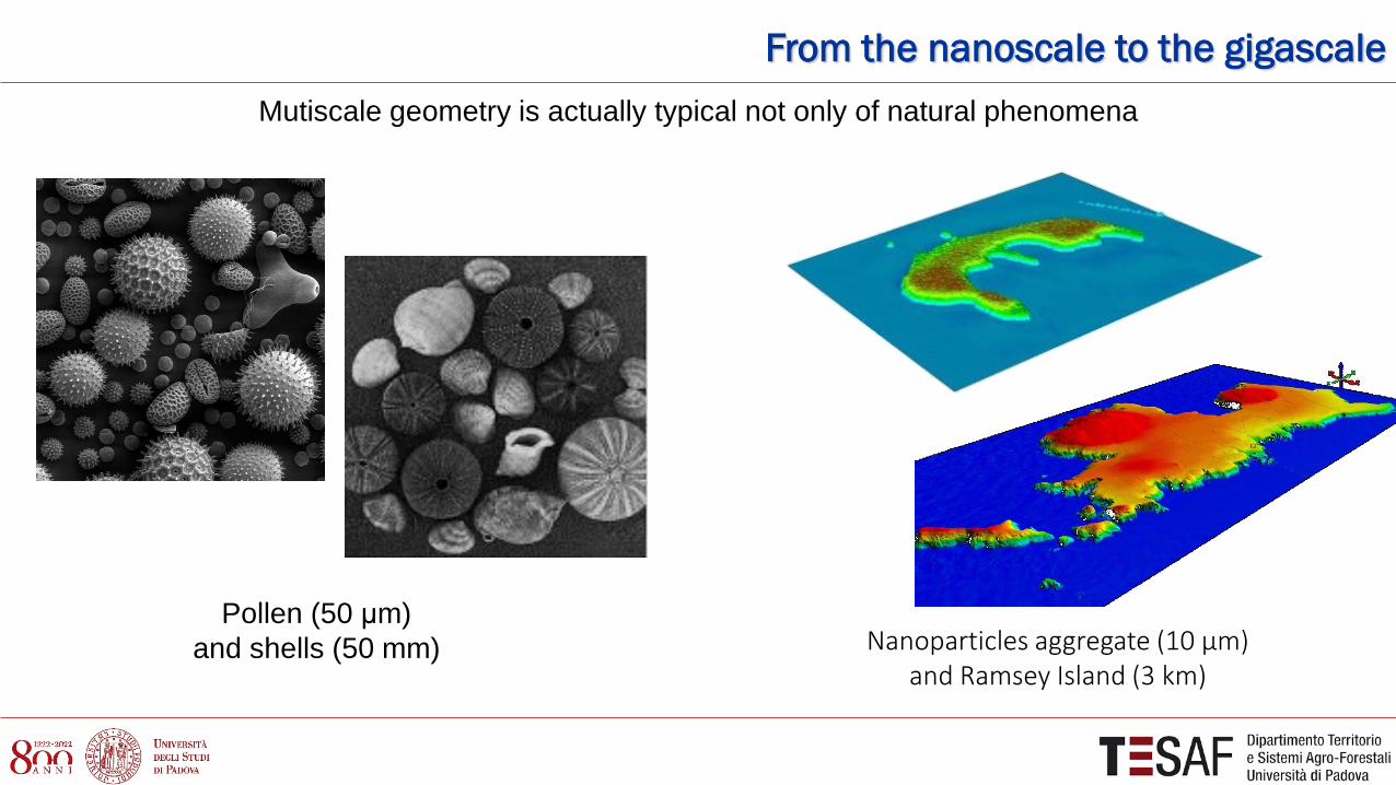
Pollen (50 μm) and shells (50 mm) Nanoparticles aggregate (10 μm)
and Ramsey Island (3 km)
From the nanoscale to the gigascale

Mutiscale geometry is actually typical not only of natural phenomena
Fracture section (1 mm) and landlside (500 m)
Nanoparticles aggregates (0,5 μm) and grizzly bear footsteps (0,2 m)
From the nanoscale to the gigascale
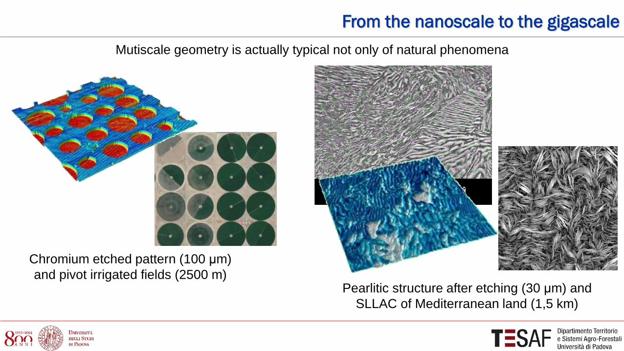
Mutiscale geometry is actually typical not only of natural phenomena
Chromium etched pattern (100 μm) and pivot irrigated fields (2500 m)
From the nanoscale to the gigascale
Pearlitic structure after etching (30 μm) and SLLAC of Mediterranean land (1,5 km)

Mutiscale of shapes is actually typical of earth phenomena
Micro-milled surface (10 μm) and ploughed soil (1 m) Fiberglass (125 μm)
and trunk section (0,8 m)
From the nanoscale to the gigascale

Etched glass (10 μm), Gravel road (1 m) and
Great Sand Dunes National Park (1 km)
From the nanoscale to the gigascale

Basic definitions
What we commonly have in common is a 2D array of pixels.
Whenever a measurement is performed and a topography is mapped, a point cloud is aquired by the instrument.
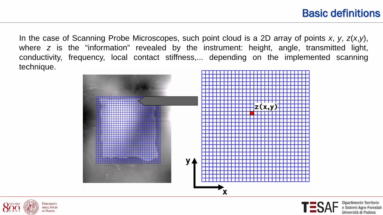
Basic definitions
In the case of Scanning Probe Microscopes, such point cloud is a 2D array of points x, y, z(x,y), where z is the “information” revealed by the instrument: height, angle, transmitted light, conductivity, frequency, local contact stiffness,... depending on the implemented scanning technique.

Basic definitions
Fast scan direction
Slow scan direction
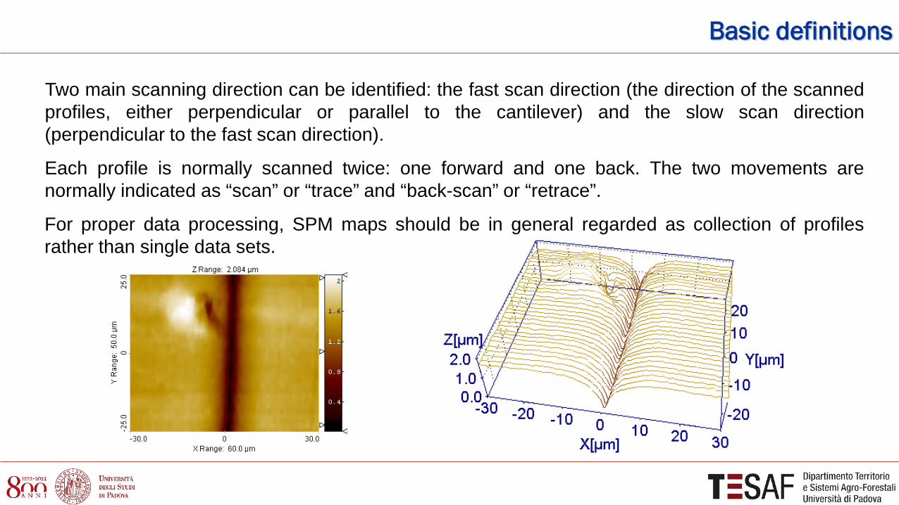
Two main scanning direction can be identified: the fast scan direction (the direction of the scanned profiles, either perpendicular or parallel to the cantilever) and the slow scan direction (perpendicular to the fast scan direction).
Each profile is normally scanned twice: one forward and one back. The two movements are normally indicated as “scan” or “trace” and “back-scan” or “retrace”.
Basic definitions
Two main scanning direction can be identified: the fast scan direction (the direction of the scanned profiles, either perpendicular or parallel to the cantilever) and the slow scan direction (perpendicular to the fast scan direction).
Each profile is normally scanned twice: one forward and one back. The two movements are normally indicated as “scan” or “trace” and “back-scan” or “retrace”.
For proper data processing, SPM maps should be in general regarded as collection of profiles rather than single data sets.

ARTIFACTS
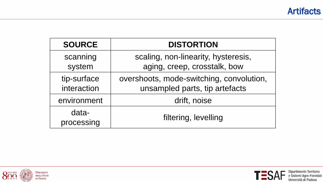
SOURCE DISTORTION scanning system
scaling, non-linearity, hysteresis, aging, creep, crosstalk, bow
tip-surface interaction
overshoots, mode-switching, convolution, unsampled parts, tip artefacts
environment drift, noise data-
processing filtering, levelling
Artifacts

During scanning distortions occur: linear distortions
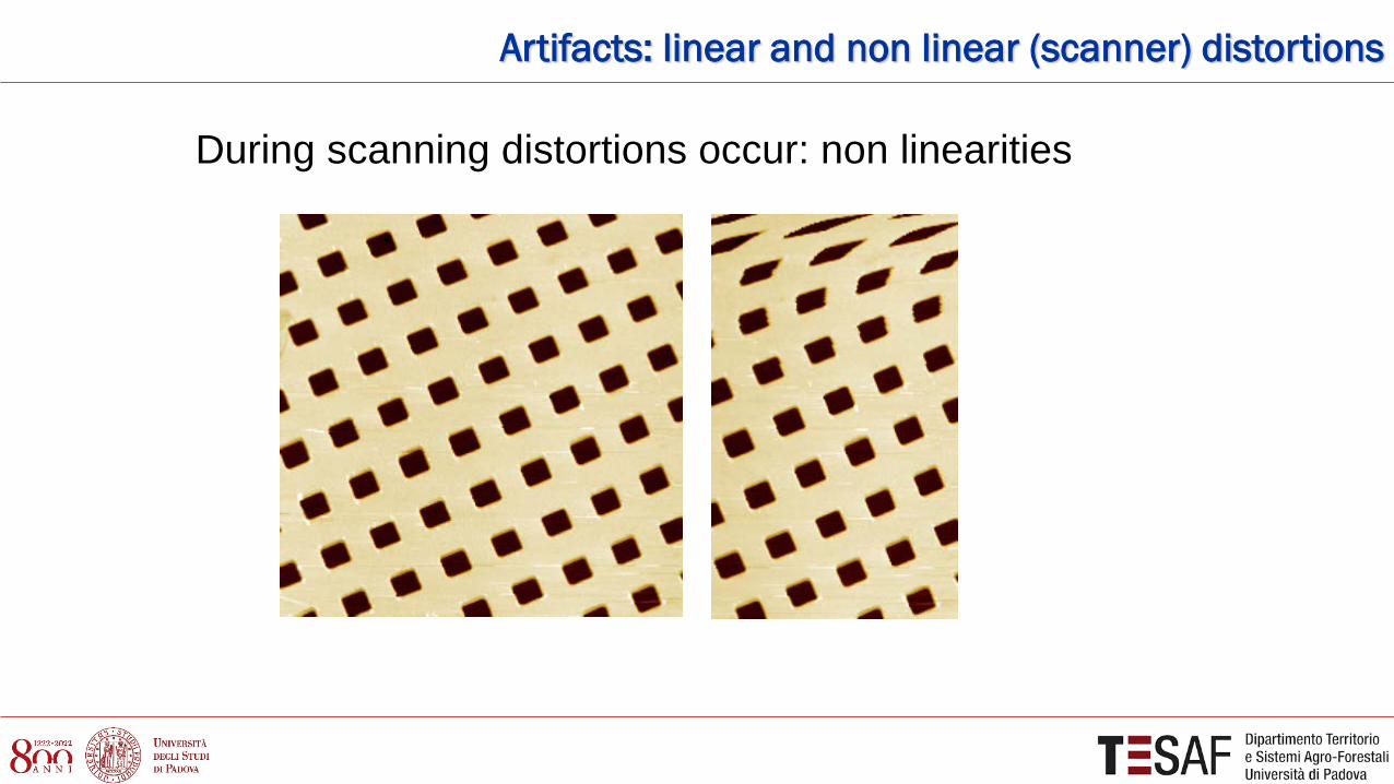
Artifacts: linear and non linear (scanner) distortions
Artifacts: linear and non linear (scanner) distortions
During scanning distortions occur: non linearities

During scanning distortions occur: hysteresis
Artifacts: linear and non linear (scanner) distortions

During scanning distortions occur: bow
Artifacts: linear and non linear (scanner) distortions
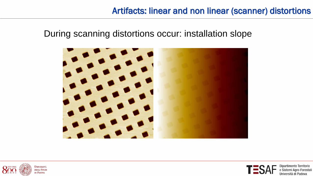
During scanning distortions occur: installation slope
Artifacts: linear and non linear (scanner) distortions
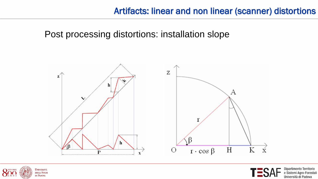
Post processing distortions: installation slope
Artifacts: linear and non linear (scanner) distortions

Post processing compensation: linear distortions
Artifacts: linear and non linear (scanner) distortions
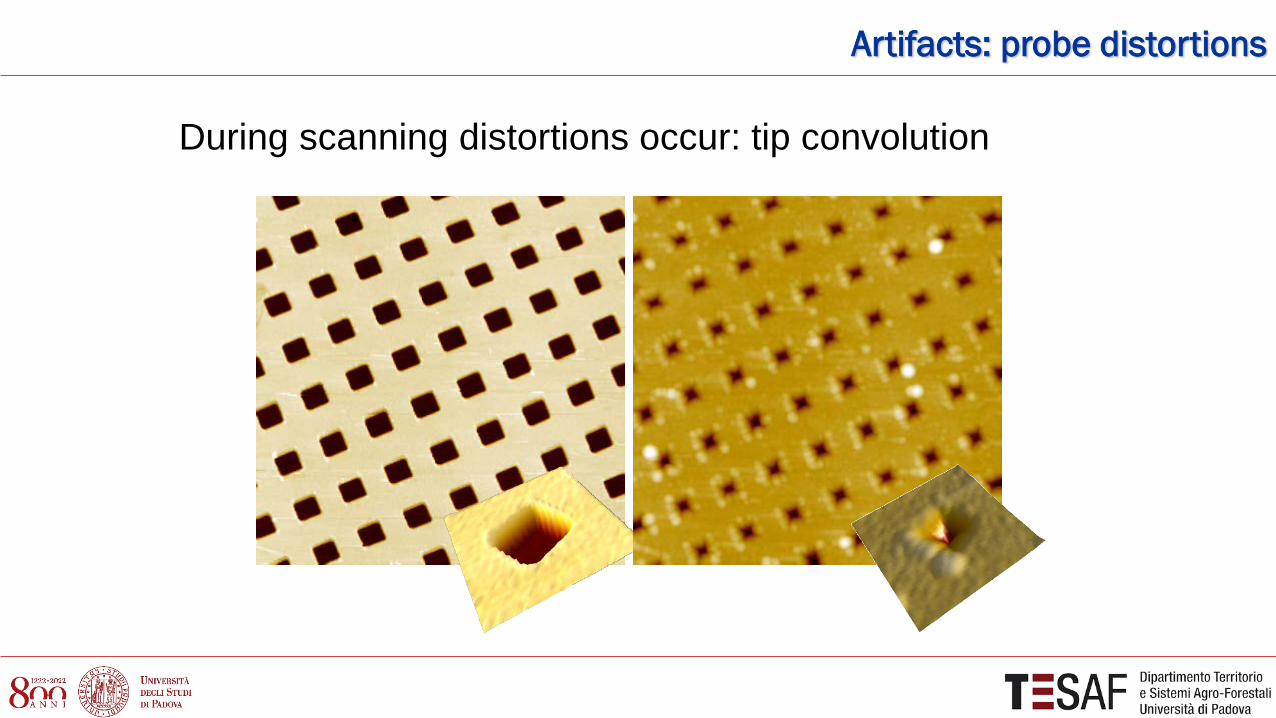
During scanning distortions occur: tip convolution
Artifacts: probe distortions
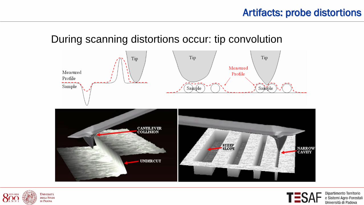
During scanning distortions occur: tip convolution
Artifacts: probe distortions
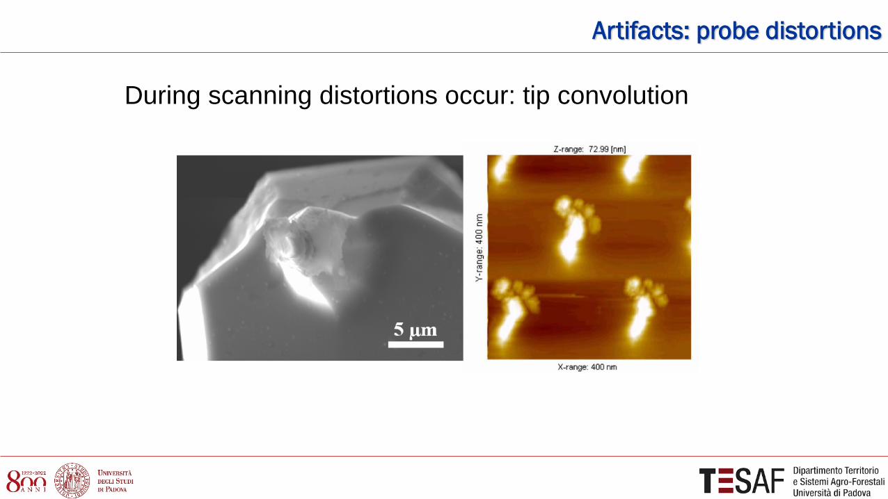
During scanning distortions occur: tip convolution
Artifacts: probe distortions
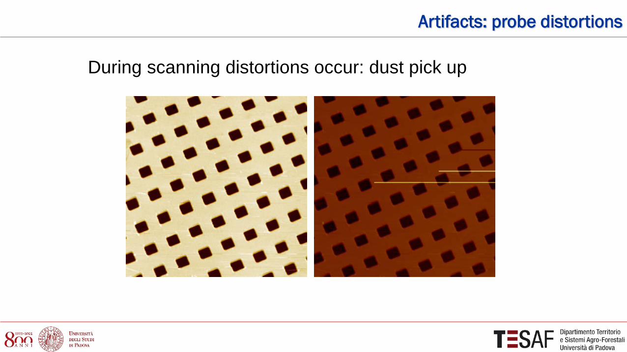
During scanning distortions occur: dust pick up
Artifacts: probe distortions

During scanning distortions occur: feedback
Typical edge artifacts: a) Overshoots, related to bad compensation of creep and hysteresis of the vertical servo control; b) feedback instability due to excessive gain and (c) smooth edge, the two terraces are far apart from each other.
a
b
c
Artifacts: probe distortions

a) Fringes around NiO structures due to mode switching; b) and c) segmentation and isolation of jumps; d) profile evidencing an apparent height level shift.
Artifacts
During scanning distortions occur: mode switching
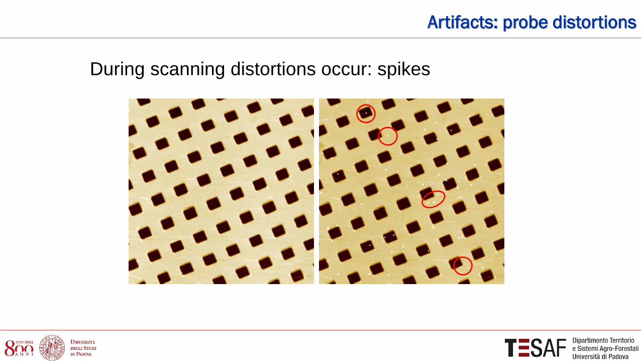
During scanning distortions occur: spikes
Artifacts: probe distortions

Environment related artifacts
During scanning distortions occur: noise
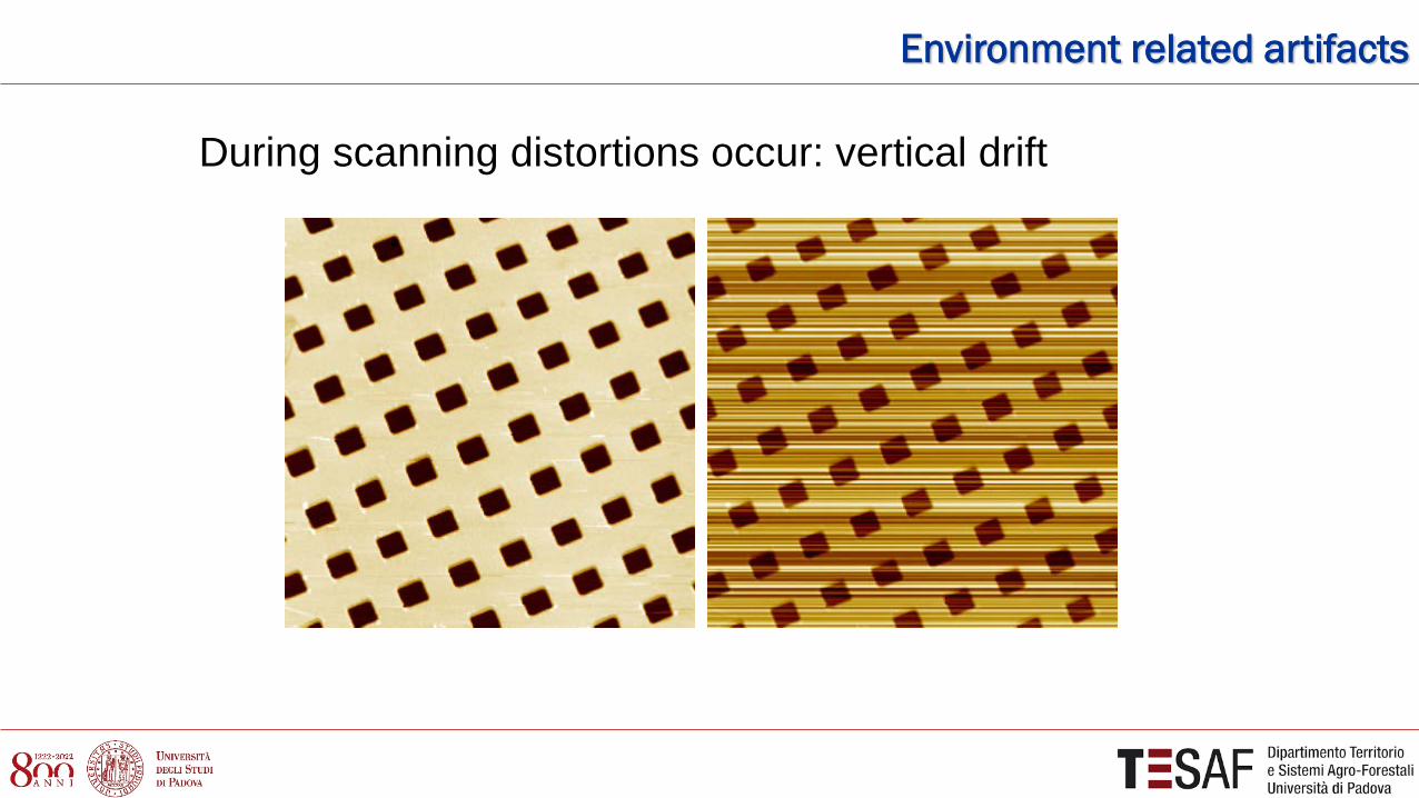
During scanning distortions occur: vertical drift
Environment related artifacts

During scanning distortions occur: horizontal drift
Environment related artifacts
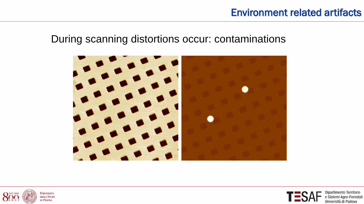
During scanning distortions occur: contaminations
Environment related artifacts

Post processing distortions: filtering
Operator artifacts

During scanning distortions occur: bad range definition
Operator artifacts

During scanning distortions occur: low resolution
Operator artifacts

APPROACH
SPM analyses approach
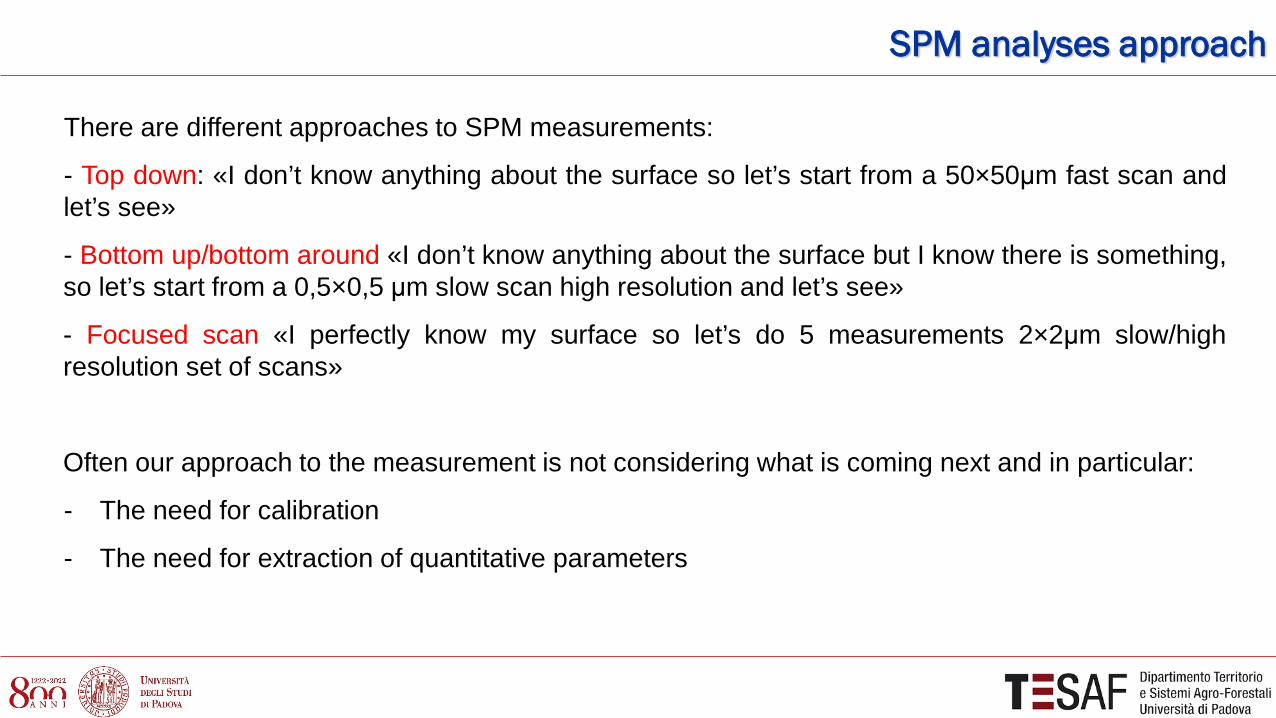
There are different approaches to SPM measurements:
- Top down: «I don’t know anything about the surface so let’s start from a 50×50μm fast scan and let’s see»
- Bottom up/bottom around «I don’t know anything about the surface but I know there is something, so let’s start from a 0,5×0,5 μm slow scan high resolution and let’s see»
- Focused scan «I perfectly know my surface so let’s do 5 measurements 2×2μm slow/high resolution set of scans»
Often our approach to the measurement is not considering what is coming next and in particular:
- The need for calibration
- The need for extraction of quantitative parameters

SPM analyses approach
Looking at published papers, different trends are recognizable among different research field (such as food packaging films, or nanoparticles), however some consideration can be done:

SPM analyses approach
Different groups of roughness parameters, including: height parameters (root mean square roughness, kurtosis, skewness,…), function related parameters (material ratio, volume,…), hybrid parameters (interfacial area ratio, root mean square gradient,…), spatial parameters (autocorrelation functions, texture direction,…)
SPM analyses approach
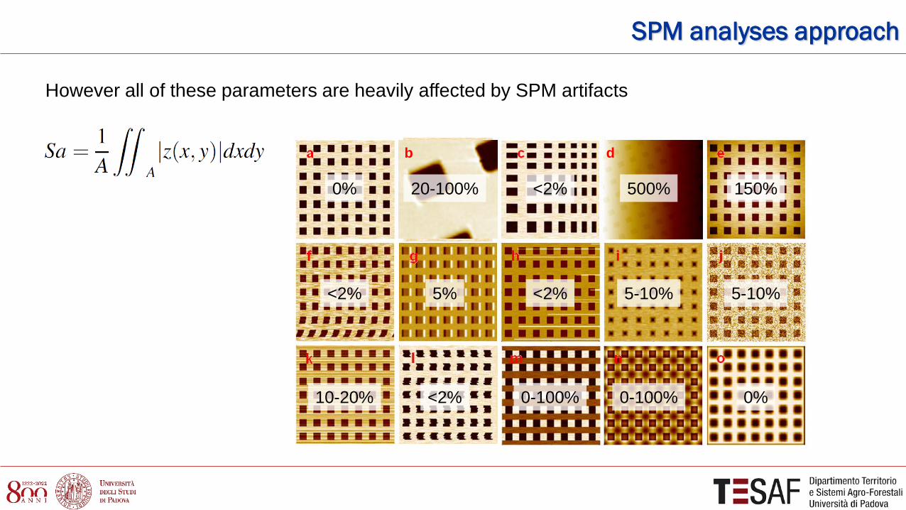
However all of these parameters are heavily affected by SPM artifacts
b
5% <2% 5-10% 5-10% <2%
<2% 0-100% 0-100% 0% 10-20%
20-100% <2% 500% 150% 0%
d

SPM analyses approach
However all of these parameters are heavily affected by SPM artifacts
b
10% 0% 10-20% <2% <2%
<2% 5-10% 10-20% 5-20% <2%
20-100% 10-20% 5% <2% 0%
d Nanoparticles diameter:
SPM analyses approach
A reasonable approach should start from 3 questions:
- Measurement: «What is the ideal trade off between the size of the features of interest, the parameters I will calculate and the time needed for the scan?»
- Calibration: «Is there any possibility of calibrating at that scanning conditions?»
- Parameters estimation: «Is there a standard method for data processing (filtering and parameter calculation)?»

SPM analyses approach
A reasonable approach should start from 3 questions:
- Measurement: «What is the ideal trade off between the size of the features of interest, the parameters I will calculate and the time needed for the scan?»
• an old rule of metrology says that at least 5 units of the feature of ineterest have to be present in the analysed area
• the parameter to be calculated should have reached a convergence
• the longer is the time, the higher is the possibility of distortions entering the masurement scan size
«true» value
extra
cted
par
amet
er
ideal window
SPM analyses approach
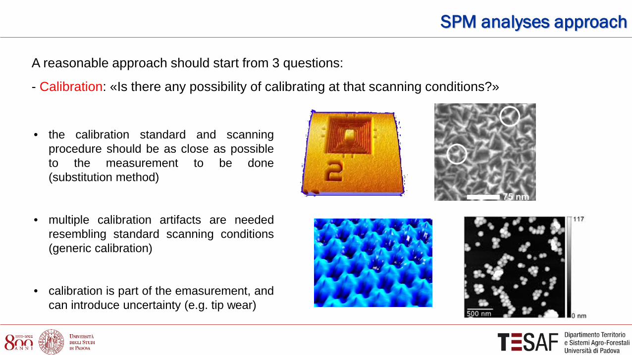
A reasonable approach should start from 3 questions:
- Calibration: «Is there any possibility of calibrating at that scanning conditions?»
• the calibration standard and scanning procedure should be as close as possible to the measurement to be done (substitution method)
• multiple calibration artifacts are needed resembling standard scanning conditions (generic calibration)
• calibration is part of the emasurement, and can introduce uncertainty (e.g. tip wear)

SPM analyses approach
A reasonable approach should start from 3 questions:
- Parameters estimation: «Is there a standard method for data processing (filtering and parameter calculation)?»
• if yes, that’s good
• if not, I need to pay attention in order to make the post processing operation as much repeatable as possible, but in this case another dilemma arises
• Higher filtering=less noise
• Lower filtering=higher repeatability

To conclude
The measurement is not the end of the story… it is just the begin
Standard procedures are needed for different SPM tasks
Scientific research should also consider clear reporting on
- Measuring procedures
- Post processing procedures
- Parameters estimation
- Uncertainty estimation

THANK YOU
Contact:
References: www.scopus.com/authid/16230574000 www.researchgate.net/profile/Francesco_Marinello publons.com/author/916340/francesco-marinello orcid.org/0000-0002-3283-5665