
ARJ December2011 Vol 102 no 4 - eolstoragewe.blob.core ...
32
Vol.102(4) December 2011 SOUTH AFRICAN INSTITUTE OF ELECTRICAL ENGINEERS 89 VOL 102 No 4 December 2011 SAIEE Africa Research Journal SAIEE AFRICA RESEARCH JOURNAL EDITORIAL STAFF ...................... IFC An Integrated Self-Sensing Approach for Active Magnetic Bearings by E.O. Ranft, G. van Schoor and C.P. du Rand.....................................90 μ-Analysis Applied to Self-Sensing Active Magnetic Bearings by P.A. van Vuuren and G. van Schoor ...................................................98 Modelling of Broadband Powerline Communication Channels by C.T. Mulangu, T.J. Afullo, and N.M. Ijumba ....................................107 System Identification of Classic HVDC Systems by L. Chetty and N.M. Ijumba............................................................... 113
Transcript of ARJ December2011 Vol 102 no 4 - eolstoragewe.blob.core ...

Vol.102(4) December 2011 SOUTH AFRICAN INSTITUTE OF ELECTRICAL ENGINEERS 89
VOL 102 No 4 December 2011
SAIEE Africa Research Journal
SAIEE AFRICA RESEARCH JOURNAL EDITORIAL STAFF ...................... IFC
An Integrated Self-Sensing Approach for Active Magnetic Bearings
by E.O. Ranft, G. van Schoor and C.P. du Rand .....................................90
μ-Analysis Applied to Self-Sensing Active Magnetic Bearings
by P.A. van Vuuren and G. van Schoor ...................................................98
Modelling of Broadband Powerline Communication Channels
by C.T. Mulangu, T.J. Afullo, and N.M. Ijumba ....................................107
System Identifi cation of Classic HVDC Systems
by L. Chetty and N.M. Ijumba ...............................................................113
Vol.102(4) December 2011SOUTH AFRICAN INSTITUTE OF ELECTRICAL ENGINEERS90
AN INTEGRATED SELF-SENSING APPROACH FOR ACTIVE MAGNETIC BEARINGS E. O. Ranft*, G. van Schoor** and C. P. du Rand* * School of Electrical, Electronic, & Computer Engineering, North-West University, Potchefstroom Campus, Private Bag X6001, Potchefstroom, 2520, South Africa E-mail: [email protected] ** Unit for Energy Systems, North-West University, Potchefstroom Campus, Private Bag X6001, Potchefstroom, 2520, South Africa E-mail: [email protected] Abstract: Self-sensing permits active magnetic bearings (AMBs) to consolidate the actuation and sensing functions into a single electromagnetic transducer. Eliminating the position sensing device as well as interfacing reduce potential system failure points, costs, and complexity. Self-sensing performance at present faces technical challenges such as magnetic cross-coupling, saturation, eddy currents, and system robustness. This work proposes an integrated self-sensing approach to collectively address mechanisms that contribute to modelling errors and position estimation inaccuracy. The self-sensing approach is based on the amplitude modulation technique and comprises a coupled reluctance network model (RNM) that is embedded in a nonlinear multiple input multiple output parameter estimator. The estimator employs a frequency-shifted model that is solved at a lower frequency to increase system performance. Furthermore, the RNM incorporates air gap fringing, complex permeability, and magnetic material nonlinearity terms. Magnetic saturation is accounted for using current scaling weights in the position estimation scheme. Basic functionality of the integrated self-sensing approach is demonstrated using an experimentally verified transient simulation model of the magnetic bearing. Verification and refinement of the RNM is accomplished through an iteration process using finite element method (FEM) results and experimental measurements. The simulation results show that the 40 node RNM can be accurate compared to an 80 000 node FEM analysis. Evaluation of the system stability margin indicates that the robustness of the magnetic bearing control is suitable for unrestricted long-term operation. Keywords: Self-sensing, active magnetic bearing (AMB), electromagnetic actuator, coupled reluctance network, position estimation.
1. INTRODUCTION Active magnetic bearings (AMBs) permit levitation of a rotor without mechanical contact at high rotational speeds, rendering them important components for modern industry. In the drive to promote wider industrial application, manufacturers and researchers aim to produce integrated AMB technology that is more reliable and economical. A self-sensing approach consolidates the actuation and sensing functions into a single electromagnetic transducer, thereby eliminating the position sensing device as well as the associated power, wiring, and interfacing. This directly reduces potential system failure points, cost, and complexity [1]. Although self-sensing offers a number of advantages over conventional displacement sensors, it remains a challenge [2]. Technical difficulties that limit self-sensing performance include eddy currents, magnetic material saturation, system robustness [2], and magnetic cross-coupling [3]. The literature describes different solutions to the magnetic saturation and cross-coupling problems. Skricka et al. [3] explores the application of a nonlinear magnetic reluctance model to reduce the effects of cross-coupling. Noh et al. [4] proposed a nonlinear parameter estimation technique to evaluate the effects of magnetic saturation.
Maslen [2] states that switching ripple amplitude is fundamental for robust self-sensing AMBs. The resulting eddy currents can be mitigated by reducing the frequency of the excitation signal [2]. This work adopts the underlying theoretical principles of these individual techniques [2-4] to form the basis for an integrated self-sensing approach. The proposed self-sensing approach aims to collectively address the mechanisms that contribute to modelling errors and position estimation inaccuracy. The solution is based on the amplitude modulation approach [5] and comprises a coupled reluctance network model (RNM) that is embedded in a nonlinear multiple input multiple output (MIMO) parameter estimator. The integrated approach implements a frequency-shifted model to reduce the computational complexity thereof. High frequency perturbations that arise from normal power amplifier (PA) switching is utilised to estimate the actuator inductance and hence, rotor displacement. Recent studies [5-8] concluded that the application of switching current ripple leads to increased robustness exceeding best achievable levels obtained by Morse et al. [9]. The accuracy of the magnetic circuit model is improved by incorporating air gap fringing, complex permeability, and magnetic material nonlinearity terms [10]. One of the difficult challenges facing self-sensing
Vol.102(4) December 2011 SOUTH AFRICAN INSTITUTE OF ELECTRICAL ENGINEERS 91
researchers [11], magnetic saturation, is addressed using current scaling weights, which permits the actuator with the lowest flux density to contribute more to the position estimate. Furthermore, a first attempt to separate position estimation of the x-and y-axis using a single coupled RNM is also presented. Verification and refinement of the RNM are accomplished through an iterative process using finite element method (FEM) results and experimental measurements. The performance limitations of the proposed self-sensing approach are investigated through simulations derived by a verified transient simulation model (TSM) of the experimental magnetic bearing.
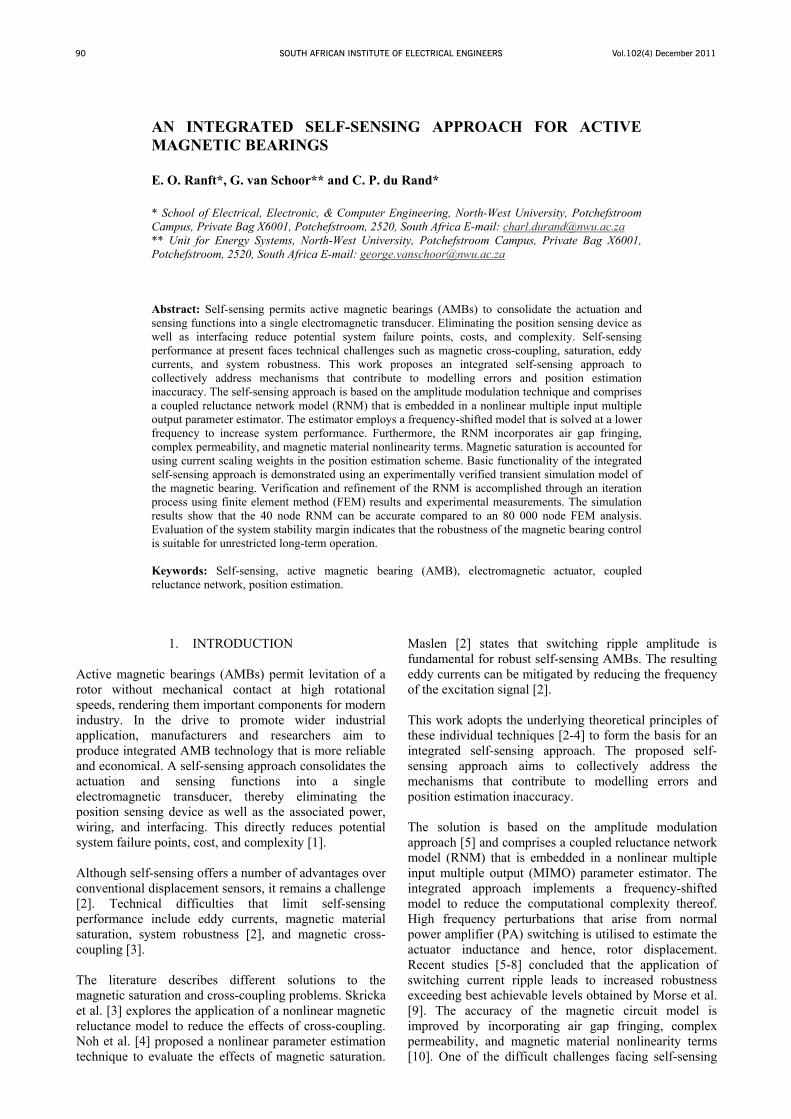
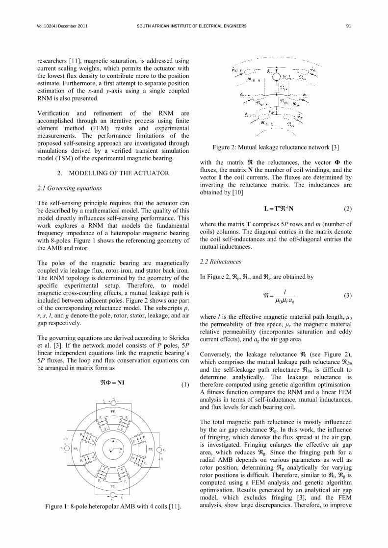
2. MODELLING OF THE ACTUATOR 2.1 Governing equations The self-sensing principle requires that the actuator can be described by a mathematical model. The quality of this model directly influences self-sensing performance. This work explores a RNM that models the fundamental frequency impedance of a heteropolar magnetic bearing with 8-poles. Figure 1 shows the referencing geometry of the AMB and rotor. The poles of the magnetic bearing are magnetically coupled via leakage flux, rotor-iron, and stator back iron. The RNM topology is determined by the geometry of the specific experimental setup. Therefore, to model magnetic cross-coupling effects, a mutual leakage path is included between adjacent poles. Figure 2 shows one part of the corresponding reluctance model. The subscripts p, r, s, l, and g denote the pole, rotor, stator, leakage, and air gap respectively. The governing equations are derived according to Skricka et al. [3]. If the network model consists of P poles, 5P linear independent equations link the magnetic bearing’s 5P fluxes. The loop and flux conservation equations can be arranged in matrix form as
Φ NIℜ = (1)
1PP
2PP
3PP
4PP
1P 2P
6P5P
3P
4P
8P
7P
y
x
SN
+ −1v
1i
N
S
2v
2i
N
NS
S
−+
− +
4i
4v
3v 3i
z
Figure 1: 8-pole heteropolar AMB with 4 coils [11].
Figure 2: Mutual leakage reluctance network [3] with the matrix the reluctances, the vector the fluxes, the matrix N the number of coil windings, and the vector I the coil currents. The fluxes are determined by inverting the reluctance matrix. The inductances are obtained by [10]
-1= ′L T Nℜ (2)
where the matrix T comprises 5P rows and m (number of coils) columns. The diagonal entries in the matrix denote the coil self-inductances and the off-diagonal entries the mutual inductances. 2.2 Reluctances In Figure 2, p, r, and s, are obtained by
0 gr
laμ μℜ = (3)
where l is the effective magnetic material path length, 0 the permeability of free space, r the magnetic material relative permeability (incorporates saturation and eddy current effects), and ag the air gap area. Conversely, the leakage reluctance (see Figure 2), which comprises the mutual leakage path reluctance and the self-leakage path reluctance , is difficult to determine analytically. The leakage reluctance is therefore computed using genetic algorithm optimisation. A fitness function compares the RNM and a linear FEM analysis in terms of self-inductance, mutual inductances, and flux levels for each bearing coil. The total magnetic path reluctance is mostly influenced by the air gap reluctance . In this work, the influence of fringing, which denotes the flux spread at the air gap, is investigated. Fringing enlarges the effective air gap area, which reduces . Since the fringing path for a radial AMB depends on various parameters as well as rotor position, determining analytically for varying rotor positions is difficult. Therefore, similar to , is computed using a FEM analysis and genetic algorithm optimisation. Results generated by an analytical air gap model, which excludes fringing [3], and the FEM analysis, show large discrepancies. Therefore, to improve
Vol.102(4) December 2011SOUTH AFRICAN INSTITUTE OF ELECTRICAL ENGINEERS92
the accuracy of the bearing model, fringing effects must be quantified. 2.3 Eddy currents The coil current ripple due to PA switching and the resulting flux ripple, produces eddy currents, which reduce the flux carrying capacity of the magnetic material. A rate dependent material permeability term is used to model this effect [10]
tanh 2( )
2fd
dss ds
σμμ μ
σμ= (4)
with = 0 r the material permeability, s the complex frequency, the electrical conductivity, and d the lamination thickness. Equation (4) together with the incremental permeability are utilised to compute the complex material permeability. The switching frequency impedance results show that the correlation between experimental measurements and the RNM, determined by (2) and (4), is not satisfactory for self-sensing. An alternative approach is explored in this work to account for eddy current effects. The complex material permeability, which is a function of flux density, is computed experimentally. A number of toroidal discs of the lamination material are stacked and excited with a switching PA through a primary coil. The switching frequency as well as flux density excursion used in the experimental magnetic bearing are employed in the setup. This approach showed marked improvement in correlation between measured and modelled results. 2.4 Magnetic material nonlinearity To account for the nonlinear behaviour of the magnetic material, the model includes the flux density dependent relative permeability μr(B). The governing equations can be written in matrix form
( ) = .NIℜ Φ Φ (5)
The curve of the nonlinear relative permeability is obtained from the peak magnetisation curve supplied by the manufacturer of the magnetic material. 2.5 Bearing model flow diagram
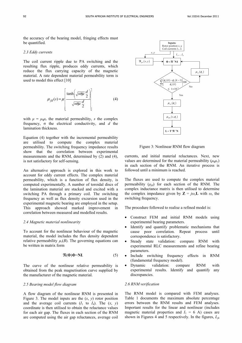
A flow diagram of the nonlinear RNM is presented in Figure 3. The model inputs are the (x, y) rotor position and the average coil currents (I1 to I4). The (x, y) coordinate is then utilised to obtain the reluctance values for each air gap. The fluxes in each section of the RNM are computed using the air gap reluctances, average coil
No
Yes
Inputs:Rotor position x, yCoil currents I1,..I4
1−= NIΦ ℜ
( ) ( )( )
5
1
6
1100
1 10
Pn n
n n
k kk
φ φφ=
−
− −
≤ ×
( ),gn x yℜ
( ),fdn nsμ φ
( )rn nμ φ
,x y1 4,I I
( )r nμ φ
1' −=L T Nℜ
Figure 3: Nonlinear RNM flow diagram currents, and initial material reluctances. Next, new values are determined for the material permeability ( 0 r) in each section of the RNM. An iterative process is followed until a minimum is reached. The fluxes are used to compute the complex material permeability ( fd) for each section of the RNM. The complex inductance matrix is then utilised to determine the complex impedance given by Z = j sL with s the switching frequency. The procedure followed to realise a refined model is: • Construct FEM and initial RNM models using
experimental bearing parameters. • Identify and quantify problematic mechanisms that
cause poor correlation. Repeat process until correspondence is satisfactory.
• Steady state validation: compare RNM with experimental RLC measurements and refine bearing parameters.
• Include switching frequency effects in RNM (fundamental frequency model).
• Dynamic validation: compare RNM with experimental results. Identify and quantify any discrepancies.
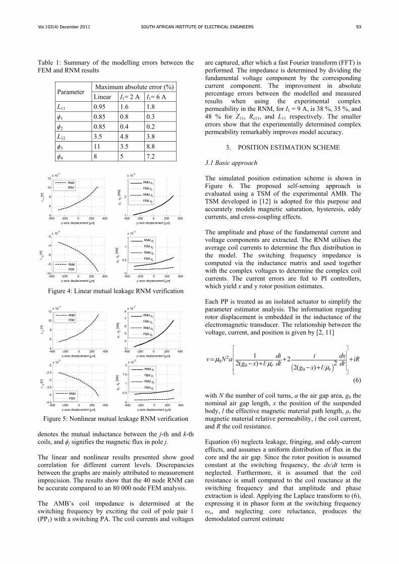
2.6 RNM verification The RNM model is compared with FEM analyses. Table 1 documents the maximum absolute percentage errors between the RNM results and FEM analyses. Important results for the linear and nonlinear (includes magnetic material properties and I1 = 6 A) cases are shown in Figures 4 and 5 respectively. In the figures, Ljk
Vol.102(4) December 2011 SOUTH AFRICAN INSTITUTE OF ELECTRICAL ENGINEERS 93
Table 1: Summary of the modelling errors between the FEM and RNM results
Parameter Maximum absolute error (%)Linear I1= 2 A I1= 6 A
L11 0.95 1.6 1.8 1 0.85 0.8 0.3 2 0.85 0.4 0.2
L12 3.5 4.8 3.8 3 11 3.5 8.8 4 8 5 7.2
Figure 4: Linear mutual leakage RNM verification
Figure 5: Nonlinear mutual leakage RNM verification
denotes the mutual inductance between the j-th and k-th coils, and j signifies the magnetic flux in pole j. The linear and nonlinear results presented show good correlation for different current levels. Discrepancies between the graphs are mainly attributed to measurement imprecision. The results show that the 40 node RNM can be accurate compared to an 80 000 node FEM analysis. The AMB’s coil impedance is determined at the switching frequency by exciting the coil of pole pair 1 (PP1) with a switching PA. The coil currents and voltages
are captured, after which a fast Fourier transform (FFT) is performed. The impedance is determined by dividing the fundamental voltage component by the corresponding current component. The improvement in absolute percentage errors between the modelled and measured results when using the experimental complex permeability in the RNM, for I1 = 9 A, is 38 %, 35 %, and 48 % for Z11, Re11, and L11 respectively. The smaller errors show that the experimentally determined complex permeability remarkably improves model accuracy.
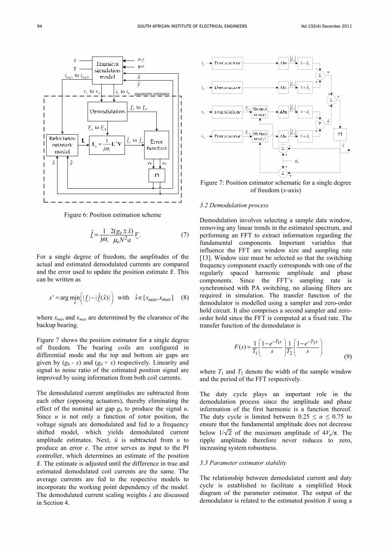
3. POSITION ESTIMATION SCHEME 3.1 Basic approach The simulated position estimation scheme is shown in Figure 6. The proposed self-sensing approach is evaluated using a TSM of the experimental AMB. The TSM developed in [12] is adopted for this purpose and accurately models magnetic saturation, hysteresis, eddy currents, and cross-coupling effects. The amplitude and phase of the fundamental current and voltage components are extracted. The RNM utilises the average coil currents to determine the flux distribution in the model. The switching frequency impedance is computed via the inductance matrix and used together with the complex voltages to determine the complex coil currents. The current errors are fed to PI controllers, which yield x and y rotor position estimates. Each PP is treated as an isolated actuator to simplify the parameter estimator analysis. The information regarding rotor displacement is embedded in the inductance of the electromagnetic transducer. The relationship between the voltage, current, and position is given by [2, 11]
( )2
00
0
1 2 22( ) 2( )rr
di i dxv N a iRg x l dt dtg x lμ μ μ
= + +− + − +
(6) with N the number of coil turns, a the air gap area, g0 the nominal air gap length, x the position of the suspended body, l the effective magnetic material path length, μr the magnetic material relative permeability, i the coil current, and R the coil resistance. Equation (6) neglects leakage, fringing, and eddy-current effects, and assumes a uniform distribution of flux in the core and the air gap. Since the rotor position is assumed constant at the switching frequency, the dx/dt term is neglected. Furthermore, it is assumed that the coil resistance is small compared to the coil reactance at the switching frequency and that amplitude and phase extraction is ideal. Applying the Laplace transform to (6), expressing it in phasor form at the switching frequency
s, and neglecting core reluctance, produces the demodulated current estimate
-400 -200 0 200 4004
6
8
10
12x 10
-3
y-axis displacement [μm]
L 11 [H
]
-400 -200 0 200 4001
2
x 10-4
y-axis displacement [μm]
φ 1 , φ 2 [
Wb]
-400 -200 0 200 400-10
-8
-6
-4
-2x 10
-5
y-axis displacement [μm]
L 12 [H
]
-400 -200 0 200 4000
0.5
1
x 10-5
y-axis displacement [μm]
φ 3 , φ 4 [
Wb]
RNMFEM
RNM φ1
FEM φ1
RNM φ2
FEM φ2
RNMFEM
RNM φ3
FEM φ3
RNM φ4
FEM φ4
-400 -200 0 200 4004
6
8
10
12x 10
-3
y-axis displacement [μm]
L 11 [H
]
-400 -200 0 200 4003
4
5
6
7
8x 10
-4
y-axis displacement [μm]
φ 1 , φ 2 [
Wb]
-400 -200 0 200 400-4.5
-4
-3.5
-3
-2.5
-2x 10
-5
y-axis displacement [μm]
L 12 [H
]
-400 -200 0 200 4000
0.5
1
1.5
2x 10
-5
y-axis displacement [μm]
φ 3 , φ 4 [
Wb]
RNMFEM
RNM φ1
FEM φ1
RNM φ2
FEM φ2
RNMFEM
RNM φ3
FEM φ3
RNM φ4
FEM φ4
Vol.102(4) December 2011SOUTH AFRICAN INSTITUTE OF ELECTRICAL ENGINEERS94
1 4toV V
1 4toI I
x y
1 4ˆ ˆtoI I11
sssjω
−=I L V
to1 4v v to1 4i i
to1 4avg avgi i xy
parameter estimator
Figure 6: Position estimation scheme
0
02
ˆ2( )1ˆ .j s
g xI VN aω μ
±= (7)
For a single degree of freedom, the amplitudes of the actual and estimated demodulated currents are compared and the error used to update the position estimate . This can be written as
ˆˆ ˆ ˆarg min | | | ( ) | with [ , ]maxminx
x I I x x x x∗ = − ∈ (8)
where xmin and xmax are determined by the clearance of the backup bearing. Figure 7 shows the position estimator for a single degree of freedom. The bearing coils are configured in differential mode and the top and bottom air gaps are given by (g0 - x) and (g0 + x) respectively. Linearity and signal to noise ratio of the estimated position signal are improved by using information from both coil currents. The demodulated current amplitudes are subtracted from each other (opposing actuators), thereby eliminating the effect of the nominal air gap g0 to produce the signal u. Since u is not only a function of rotor position, the voltage signals are demodulated and fed to a frequency shifted model, which yields demodulated current amplitude estimates. Next, û is subtracted from u to produce an error e. The error serves as input to the PI controller, which determines an estimate of the position
. The estimate is adjusted until the difference in true and estimated demodulated coil currents are the same. The average currents are fed to the respective models to incorporate the working point dependency of the model. The demodulated current scaling weights are discussed in Section 4.
2i
4i
2v
4v
0g
2I
4I
2V
4V
2I
4I
e
u
u
x
−
+
−
+
+
−
+
+
−
+
1 xλ+
1 xλ−
1 xλ+
1 xλ−
Figure 7: Position estimator schematic for a single degree of freedom (x-axis)
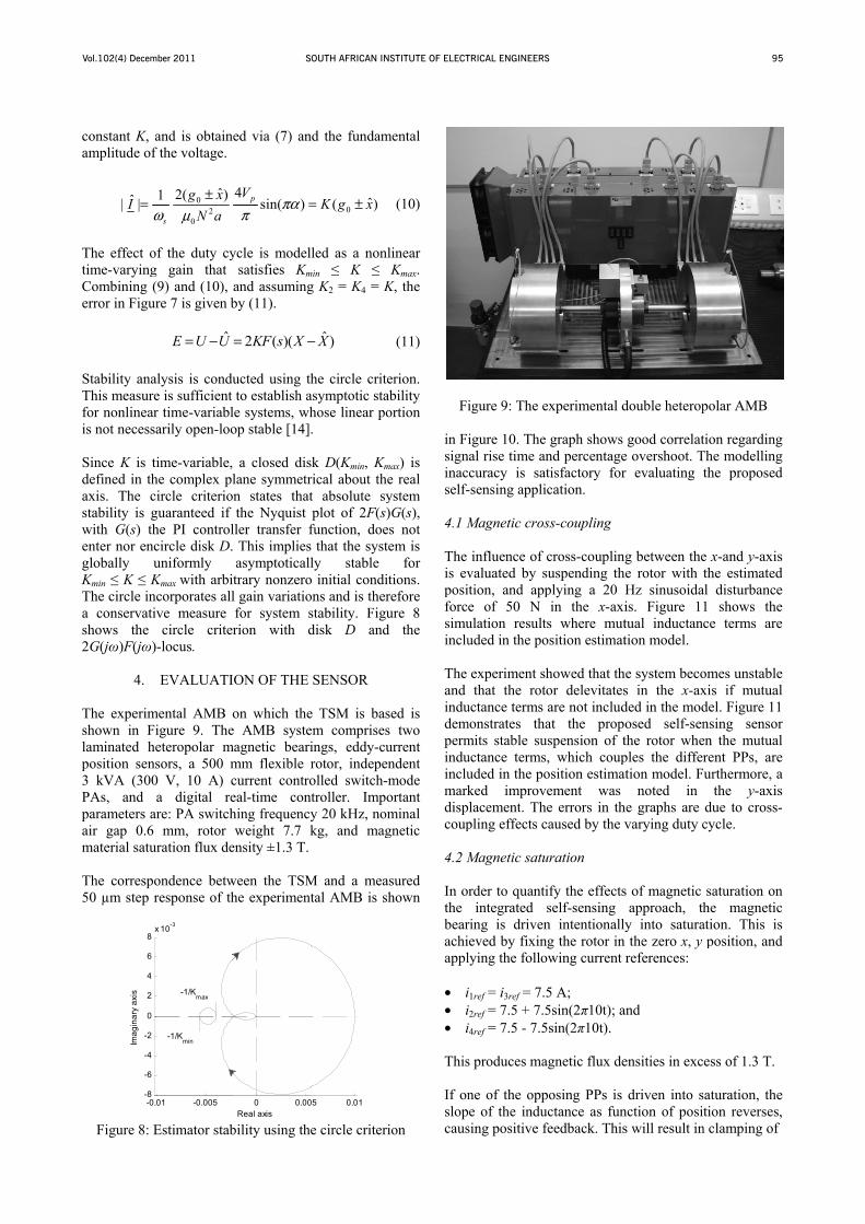
3.2 Demodulation process Demodulation involves selecting a sample data window, removing any linear trends in the estimated spectrum, and performing an FFT to extract information regarding the fundamental components. Important variables that influence the FFT are window size and sampling rate [13]. Window size must be selected so that the switching frequency component exactly corresponds with one of the regularly spaced harmonic amplitude and phase components. Since the FFT’s sampling rate is synchronised with PA switching, no aliasing filters are required in simulation. The transfer function of the demodulator is modelled using a sampler and zero-order hold circuit. It also comprises a second sampler and zero-order hold since the FFT is computed at a fixed rate. The transfer function of the demodulator is
1 2
1 2
1 1 1 1( )T s T se eF s T s T s
− −− −= (9)
where T1 and T2 denote the width of the sample window and the period of the FFT respectively. The duty cycle plays an important role in the demodulation process since the amplitude and phase information of the first harmonic is a function thereof. The duty cycle is limited between 0.25 0.75 to ensure that the fundamental amplitude does not decrease below 1/ of the maximum amplitude of 4Vp/ . The ripple amplitude therefore never reduces to zero, increasing system robustness. 3.3 Parameter estimator stability The relationship between demodulated current and duty cycle is established to facilitate a simplified block diagram of the parameter estimator. The output of the demodulator is related to the estimated position using a
Vol.102(4) December 2011 SOUTH AFRICAN INSTITUTE OF ELECTRICAL ENGINEERS 95
constant K, aamplitude of
ˆ| |Iω
=
The effect otime-varyingCombining (error in Figur
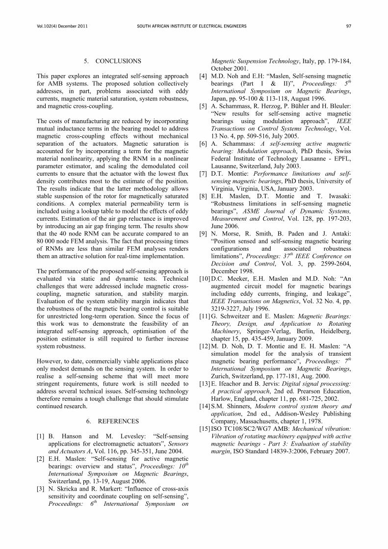
Stability anaThis measurefor nonlinearis not necess Since K is tdefined in thaxis. The cstability is gwith G(s) thenter nor encglobally uKmin K KThe circle ina conservatishows the 2G(j )F(j )
4. The experimshown in Filaminated heposition sens3 kVA (300PAs, and parameters aair gap 0.6 material satu The correspo50 μm step r
Figure 8: E
-0.-8
-6
-4
-2
0
2
4
6
8x
Imag
inar
y ax
isand is obtaine
f the voltage.
02
0
ˆ2( )1
s
g xN aω μ
±
of the duty cyg gain that (9) and (10), are 7 is given b
ˆE U U= − =
alysis is condue is sufficient r time-variablarily open-loo
time-variable, he complex plcircle criterionguaranteed if he PI controlcircle disk D. uniformly Kmax with arbitncorporates allive measure
circle criter)-locus.
EVALUATI
mental AMB oigure 9. Theeteropolar msors, a 500 m
0 V, 10 A) ca digital re
are: PA switchmm, rotor
uration flux de
ondence betwresponse of th
Estimator stab
.01 -0.005
x 10-3
-1/Kmin
-1/Kmax
ed via (7) and
4sin( )pV
παπ
=
ycle is modellsatisfies Km
and assumingby (11).
2 ( )(KF s X= −
ucted using thto establish ae systems, wh
op stable [14].
a closed disklane symmetrn states thatthe Nyquist
ller transfer fThis implies asymptoticalltrary nonzerol gain variatiofor system srion with d
ON OF THE
on which thee AMB syste
magnetic bearimm flexible rcurrent controeal-time conthing frequencyweight 7.7 k
ensity ±1.3 T.
ween the TSMhe experiment
bility using the
0 0.00Real axis
d the fundam
0 ˆ( )K g x= ±
led as a nonlmin K g K2 = K4 = K
ˆ )X−
he circle criteasymptotic stabhose linear po.
k D(Kmin, Kmrical about thet absolute syplot of 2F(s)
function, doesthat the syste
ly stable initial conditns and is ther
stability. Figudisk D and
SENSOR
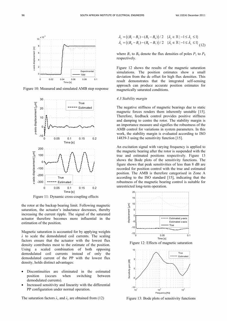
e TSM is basm comprisesings, eddy-curotor, indepenolled switch-mtroller. Impoy 20 kHz, nomkg, and mag
M and a meastal AMB is sh
e circle criteri
5 0.01
mental
(10)
linear Kmax.
K, the
(11)
erion. bility
ortion
max) is e real ystem G(s), s not em is
for tions. refore ure 8
the
ed is two
urrent ndent mode ortant minal gnetic
sured hown
ion
Fi
in Fisigninacself- 4.1 M The is evposiforcsimuinclu The and indudemperminduinclumarkdispcoup 4.2 M In othe bearachiappl • i• i• i This If onslopcaus
igure 9: The e
igure 10. The nal rise time ancuracy is sat-sensing appli
Magnetic cros
influence of valuated by stion, and appe of 50 N ulation resultuded in the po
experiment shthat the roto
uctance terms monstrates thamits stable suuctance termsuded in the poked improvlacement. Thpling effects c
Magnetic satu
rder to quantiintegrated
ring is driveneved by fixinlying the follo
i1ref = i3ref = 7.5i2ref = 7.5 + 7.5i4ref = 7.5 - 7.5
s produces ma
ne of the oppe of the indu
sing positive f
experimental d
graph shows nd percentagetisfactory forcation.
ss-coupling
cross-couplinsuspending thplying a 20 in the x-axi
s where mutosition estimat
howed that thor delevitatesare not includat the prop
uspension of t, which couposition estimaement was e errors in th
caused by the v
uration
ify the effectsself-sensing n intentionally
ng the rotor inowing current
5 A; 5sin(2 10t); a5sin(2 10t).
agnetic flux de
posing PPs is uctance as funfeedback. This
double heterop
good correlate overshoot. Tr evaluating
g between thehe rotor with Hz sinusoidais. Figure 1tual inductantion model.
he system becos in the x-axded in the modosed self-senthe rotor wheples the diffeation model. F
noted in he graphs are varying duty c
s of magnetic approach, th
y into saturan the zero x, y
references:
and
ensities in exc
driven into snction of posis will result in
polar AMB
tion regardingThe modellingthe proposed
e x-and y-axisthe estimated
al disturbance1 shows thece terms are
omes unstablexis if mutualdel. Figure 11nsing sensoren the mutualrent PPs, are
Furthermore, athe y-axis
due to cross-cycle.
saturation onhe magnetic
ation. This isposition, and
cess of 1.3 T.
saturation, theition reverses,n clamping of
g g d
s d e e e
e l
r l e a s -
n c s d
e ,
Vol.102(4) December 2011SOUTH AFRICAN INSTITUTE OF ELECTRICAL ENGINEERS96
Figure 10: Measured and simulated AMB step response
Figure 11: Dynamic cross-coupling effects
the rotor at the backup bearing limit. Following magnetic saturation, the actuator’s inductance decreases, thereby increasing the current ripple. The signal of the saturated actuator therefore becomes more influential in the estimation of the position. Magnetic saturation is accounted for by applying weights to scale the demodulated coil currents. The scaling
factors ensure that the actuator with the lowest flux density contributes most to the estimate of the position. Using a scaled combination of both opposing demodulated coil currents instead of only the demodulated current of the PP with the lowest flux density, holds distinct advantages: • Discontinuities are eliminated in the estimated
position (occurs when switching between demodulated currents).
• Increased sensitivity and linearity with the differential PP configuration under normal operation.
The saturation factors x and y are obtained from (12)
( )( )
1 2 5 6
4 3 8 7
( ) ( ) / 2 { | 1 1}( ) ( ) / 2 { | 1 1}
y y y
x x x
B B B BB B B B
λ λ λλ λ λ
= − − − ∈ − ≤ ≤= − − − ∈ − ≤ ≤ (12)
where B1 to B8 denote the flux densities of poles P1 to P8 respectively. Figure 12 shows the results of the magnetic saturation simulations. The position estimates show a small deviation from the dc offset for high flux densities. This result demonstrates that the integrated self-sensing approach can produce accurate position estimates for magnetically saturated conditions. 4.3 Stability margin The negative stiffness of magnetic bearings due to static magnetic forces renders them inherently unstable [15]. Therefore, feedback control provides positive stiffness and damping to centre the rotor. The stability margin is an importance measure and signifies the robustness of the AMB control for variations in system parameters. In this work, the stability margin is evaluated according to ISO 14839-3 using the sensitivity function [15]. An excitation signal with varying frequency is applied to the magnetic bearing after the rotor is suspended with the true and estimated positions respectively. Figure 13 shows the Bode plots of the sensitivity functions. The figure shows that peak sensitivities of less than 8 dB are recorded for position control with the true and estimated position. The AMB is therefore categorised in Zone A according to the ISO standard [15], indicating that the robustness of the magnetic bearing control is suitable for unrestricted long-term operation.
Figure 12: Effects of magnetic saturation
Figure 13: Bode plots of sensitivity functions
0 0.02 0.04 0.06 0.08 0.1
0
2
4
6
8
10x 10-5
Time [s]
x-a
xis
disp
lace
men
t [m
]
ExperimentalTSM
0 0.05 0.1 0.15 0.2-10
0
10
20
30
Time [s]
y-ax
is d
ispl
acem
ent [
μm]
TrueEstimated
0 0.05 0.1 0.15 0.2
-300
-200
-100
0
100
200
Time [s]
x-ax
is d
ispl
acem
ent [
μm]
TrueEstimated
0 0.05 0.1-15
-10
-5
0
5
10
15
20
Time [s]
disp
lace
men
t [μm
]
Estimated y-axisEstimated x-axisTrue
101 102 103-10
-5
0
5
10
Frequency [Hz]
Sen
sitiv
ity g
ain
[dB
]
TrueEstimated
Vol.102(4) December 2011 SOUTH AFRICAN INSTITUTE OF ELECTRICAL ENGINEERS 97
5. CONCLUSIONS This paper explores an integrated self-sensing approach for AMB systems. The proposed solution collectively addresses, in part, problems associated with eddy currents, magnetic material saturation, system robustness, and magnetic cross-coupling. The costs of manufacturing are reduced by incorporating mutual inductance terms in the bearing model to address magnetic cross-coupling effects without mechanical separation of the actuators. Magnetic saturation is accounted for by incorporating a term for the magnetic material nonlinearity, applying the RNM in a nonlinear parameter estimator, and scaling the demodulated coil currents to ensure that the actuator with the lowest flux density contributes most to the estimate of the position. The results indicate that the latter methodology allows stable suspension of the rotor for magnetically saturated conditions. A complex material permeability term is included using a lookup table to model the effects of eddy currents. Estimation of the air gap reluctance is improved by introducing an air gap fringing term. The results show that the 40 node RNM can be accurate compared to an 80 000 node FEM analysis. The fact that processing times of RNMs are less than similar FEM analyses renders them an attractive solution for real-time implementation. The performance of the proposed self-sensing approach is evaluated via static and dynamic tests. Technical challenges that were addressed include magnetic cross-coupling, magnetic saturation, and stability margin. Evaluation of the system stability margin indicates that the robustness of the magnetic bearing control is suitable for unrestricted long-term operation. Since the focus of this work was to demonstrate the feasibility of an integrated self-sensing approach, optimisation of the position estimator is still required to further increase system robustness. However, to date, commercially viable applications place only modest demands on the sensing system. In order to realise a self-sensing scheme that will meet more stringent requirements, future work is still needed to address several technical issues. Self-sensing technology therefore remains a tough challenge that should stimulate continued research.
6. REFERENCES [1] B. Hanson and M. Levesley: “Self-sensing
applications for electromagnetic actuators”, Sensors and Actuators A, Vol. 116, pp. 345-351, June 2004.
[2] E.H. Maslen: “Self-sensing for active magnetic bearings: overview and status”, Proceedings: 10th International Symposium on Magnetic Bearings, Switzerland, pp. 13-19, August 2006.
[3] N. Skricka and R. Markert: “Influence of cross-axis sensitivity and coordinate coupling on self-sensing”, Proceedings: 6th International Symposium on
Magnetic Suspension Technology, Italy, pp. 179-184, October 2001.
[4] M.D. Noh and E.H: “Maslen, Self-sensing magnetic bearings (Part I & II)”, Proceedings: 5th International Symposium on Magnetic Bearings, Japan, pp. 95-100 & 113-118, August 1996.
[5] A. Schammass, R. Herzog, P. Bühler and H. Bleuler: “New results for self-sensing active magnetic bearings using modulation approach”, IEEE Transactions on Control Systems Technology, Vol. 13 No. 4, pp. 509-516, July 2005.
[6] A. Schammass: A self-sensing active magnetic bearing: Modulation approach, PhD thesis, Swiss Federal Institute of Technology Lausanne - EPFL, Lausanne, Switzerland, July 2003.
[7] D.T. Montie: Performance limitations and self-sensing magnetic bearings, PhD thesis, University of Virginia, Virginia, USA, January 2003.
[8] E.H. Maslen, D.T. Montie and T. Iwasaki: “Robustness limitations in self-sensing magnetic bearings”, ASME Journal of Dynamic Systems, Measurement and Control, Vol. 128, pp. 197-203, June 2006.
[9] N. Morse, R. Smith, B. Paden and J. Antaki: “Position sensed and self-sensing magnetic bearing configurations and associated robustness limitations”, Proceedings: 37th IEEE Conference on Decision and Control, Vol. 3, pp. 2599-2604, December 1998.
[10] D.C. Meeker, E.H. Maslen and M.D. Noh: “An augmented circuit model for magnetic bearings including eddy currents, fringing, and leakage”, IEEE Transactions on Magnetics, Vol. 32 No. 4, pp. 3219-3227, July 1996.
[11] G. Schweitzer and E. Maslen: Magnetic Bearings: Theory, Design, and Application to Rotating Machinery, Springer-Verlag, Berlin, Heidelberg, chapter 15, pp. 435-459, January 2009.
[12] M. D. Noh, D. T. Montie and E. H. Maslen: “A simulation model for the analysis of transient magnetic bearing performance”, Proceedings: 7th International Symposium on Magnetic Bearings, Zurich, Switzerland, pp. 177-181, Aug. 2000.
[13] E. Ifeachor and B. Jervis: Digital signal processing: A practical approach, 2nd ed. Prearson Education, Harlow, England, chapter 11, pp. 681-725, 2002.
[14] S.M. Shinners, Modern control system theory and application, 2nd ed., Addison-Wesley Publishing Company, Massachusetts, chapter 1, 1978.
[15] ISO TC108/SC2/WG7 AMB: Mechanical vibration: Vibration of rotating machinery equipped with active magnetic bearings - Part 3: Evaluation of stability margin, ISO Standard 14839-3:2006, February 2007.
Vol.102(4) December 2011SOUTH AFRICAN INSTITUTE OF ELECTRICAL ENGINEERS98
μ-ANALYSIS APPLIED TO SELF-SENSING ACTIVE MAGNETICBEARINGS
P.A. van Vuuren ∗ and G. van Schoor †
∗ School of Electrical, Electronic and Computer Engineering, North-West University, Private BagX6001, Potchefstroom, 2520, South-Africa. E-mail: [email protected]† E-mail: [email protected]
Abstract: The stability margin of a two degree-of-freedom self-sensing active magnetic bearing (AMB)is estimated by means of μ-analysis. The specific self-sensing algorithm implemented in this studyis the direct current measurement method. Detailed black-box models are developed for the mainsubsystems in the AMB by means of discrete-time system identification. In order to obtain modelsfor dynamic uncertainty in the various subsystems in the AMB, the identified models are combinedto form a closed-loop model for the self-sensing AMB. The response of this closed-loop model isthen compared to the original AMB’s response and models for the dynamic uncertainty are empiricallydeduced. Finally, the system’s stability margin for the modelled uncertainty is estimated by means ofμ-analysis. The results show that μ-analysis is ill-equipped to estimate the stability margin of a nonlinearsystem.
Key words: Active magnetic bearings, system identification, self-sensing, μ-analysis
1. INTRODUCTION
In contrast with conventional bearings, active magneticbearings (AMBs) use actively controlled magnetic forcesto ensure contactless support of a rotating axle. AnAMB consists of non-contact position sensors, adigital controller, power amplifiers and a stator withelectromagnets. These components and the generalstructure of an AMB are summarized in [1].
Accurate and reliable position sensors form criticalcomponents of a functioning AMB system. These sensorsare however expensive. Self-sensing techniques attemptto estimate the position of the rotor from the electricalimpedance of the stator electromagnet coils [2].
For self-sensing AMBs to be of practical worth, they haveto be robust. Robustness analysis aims to quantify a controlsystem’s tolerance for uncertainty. This uncertainty ingeneral encompasses any deviation of the mathematicalmodel from the physical reality. Uncertainties surroundingthe model can be broadly classified into parametricuncertainty and dynamic uncertainty. Parametricuncertainty is applicable when the system’s model isaccurate with the exception of a few parameters whoseprecise values aren’t known [3]. In contrast, dynamicuncertainty describes the situation when the system’smodel is inaccurate due to unmodelled dynamics [3].
The de facto standard for robustness estimation in theAMB literature is the sensitivity function [4], [5] and[6]. Acceptance of the draft ISO standard∗ for theevaluation of the stability of rotating machinery equippedwith AMBs [7] isn’t unanimous in the AMB researchcommunity. In [8] it is argued that the peak value of
∗This draft standard uses the sensitivity function to assess the
robustness of AMBs.
the sensitivity function only gives a necessary (but notsufficient) condition for robust stability. Their theoreticalarguments were also supported by practical examples ofAMB suspended systems that met the criteria set out bythe draft ISO standard, yet became unstable due to modalvariations or gyroscopic coupling.
Alternative multiple-input, multiple-output (MIMO) ro-bustness estimation techniques that have been appliedto AMBs include the generalized Nyquist criterion [9],Kharitonov’s stability theorem [9] and the ν-gap metric[10]. Of the available LTI MIMO robustness estimationtechniques, μ-analysis holds out the promise of deliveringthe least conservative estimates of the stability margin ofan AMB system. Although μ-synthesis has been applied todesign controllers for AMB systems (e.g. [11] and [10]),μ-analysis curiously has never been used to assess therobustness of AMBs.
Robustness analysis techniques have played a pivotal rolein the debate on the viability of self-sensing AMBs. Afterthe development of state-estimator self-sensing AMBs,Kucera showed by means of a sensitivity analysis thatsuch self-sensing AMBs are quite sensitive for parametricuncertainty [12]. Following this result, Morse et al.used the sensitivity function to prove that self-sensing ingeneral has fundamental theoretical limits on its stabilityrobustness [13]. These negative results were however sooncontradicted by various researchers (e.g. [4]) who showedthat practical modulation based self-sensing AMBs canbe almost as robust as sensed AMBs (according to theproposed ISO standard).
The apparent contradiction between the theory andpractical results on the robustness of self-sensing AMBswas addressed by Maslen et al. [14] and [15]. Theyfound that it is essential to include the switching ripple
Vol.102(4) December 2011 SOUTH AFRICAN INSTITUTE OF ELECTRICAL ENGINEERS 99
component of the coil current in the AMB model that issubjected to robustness analysis. Accurate modelling ofswitching power amplifiers requires nonlinear time-variantmodels.
One of the lessons from [13], [14] and [15] is thataccurate robustness analysis requires that each of theconstituent parts of a self-sensing AMB system bemodelled accurately. The fundamental prerequisite forμ-analysis is however that the system under scrutiny bemodelled with an analytical LTI model. Fortunately,it is possible for LTI black-box models obtained viasystem identification to closely approximate the oscillatorybehaviour of switching power amplifiers if the order ischosen sufficiently high. Another advantage of systemidentification is that it doesn’t have any trouble inmodelling cross-coupling occurring in a system. This is ahuge benefit since electromagnetic cross-coupling also hasa large effect on self-sensing implemented on heteropolarAMBs [16], [5]. Furthermore, it is quite difficult toobtain an accurate analytical model for electromagneticcross-coupling in an AMB stator by means of firstprinciples deductive modelling techniques. The potentialpitfalls of applying system identification to AMBs arehighlighted in [1]. The most important lesson from [1]is that the excitation signal used for system identificationmust be constructed wisely in order to ensure that an LTImodel is obtained.
Robustness analysis of self-sensing AMBs by meansof μ-analysis therefore requires that detailed black-boxmodels are developed for the main subsystems in the AMBby means of discrete-time system identification. Accurateμ-analysis requires accurate models of the nominal systemas well as the uncertainty to which the model is subjected[3]. For this reason system identification is also applied toobtain accurate models for the dynamic uncertainty in theself-sensing AMB system.
Although the basic idea (namely of performing μ-analysison the basis of models obtained via system identification)isn’t new, it is the first time that it has been applied toself-sensing AMBs. The closest prior work in this generalfield was however confined to SISO systems in the processcontrol industry [17], [18].
This paper’s focus is on a 2-DOF self-sensing AMB. Thedependency of self-sensing on an accurate representationof the ripple current in turn requires that the self-sensingmodule, AMB plant and power ampifier models beseparately obtained by means of system identification.This is in contrast with the standard practice of systemidentification in the AMB literature, namely of includingeverything except the controller in the plant model [19],[20], [21] and [22].
The rest of this paper starts off with a summary of thespecific version of self-sensing under scrutiny, namely thedirect current measurement (DCM) method. Section 3discusses the application of system identification to obtaindiscrete-time models for each of the main components
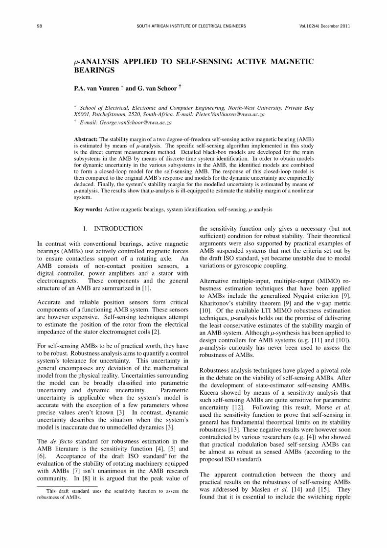
Figure 1: Magnetic circuit of a 1-DOF AMB
of the self-sensing AMB. Next, section 4 summarizesthe application of μ-analysis by means of a case study,namely the robustness analysis of the AMB for dynamicuncertainty in the self-sensing module. Following this, theprocedure with which dynamic uncertainty in the AMBplant and self-sensing module can be modelled is brieflydescribed in section 5. Lastly, section 6 contains theresults of simulation studies on μ-analysis applied to assessthe effect of various forms of uncertainty on the stabilitymargin of the self-sensing AMB.
2. THE DCM SELF-SENSING AMB
2.1 Introduction to DCM self-sensing
Self-sensing capitalizes on the principle that the inductanceof an AMB stator coil is influenced by the size of theairgap. To see how the impedance of an AMB coil isinfluenced by the airgap take for example the magneticcircuit of a one degree-of-freedom (1-DOF) AMB in figure1 [4].
To simplify the analysis, eddy current effects are neglected(as well as magnetic leakage and fringing). Furthermore,it is assumed that the magnetic flux has a uniformdistribution throughout the magnetic circuit. By makinguse of the laws of Faraday, Ohm and Ampere, therelationship between the coil voltage v(t) and current i(t)is given by (1) [23],
v(t) =(
μ0N2A2xg(t)+ lc/μr
)di(t)
dt−
2
(μ0N2Ai(t)
(2xg(t)+ lc/μr)2
)dxg(t)
dt+ i(t)R, (1)
where μ0 is the permeability of free space; N is the numberof turns in the coil; A is the pole-face area; xg is thedistance of the airgap between the stator and rotor; lc is thelength of the magnetic path (excluding the airgap); μr isthe relative permeability of the AMB stator; and R denotesthe electrical resistance of the coil wire.
Vol.102(4) December 2011SOUTH AFRICAN INSTITUTE OF ELECTRICAL ENGINEERS100
Clearly, the relationship between the coil voltage andcurrent is influenced by the instantaneous position of therotor within the airgap.
DCM self-sensing stems from the fact that the rotorposition is directly related to the peak value of theripple current during a switching cycle. This becomesobvious when (1) is simplified further to its bare essentials.By neglecting the coil resistance, as well as nonlinearmagnetic effects and assuming that the AMB rotor movesvery slowly compared to the rapid variation in the coilcurrent, the airgap can be expressed as follows [5]:
xg(t) =(
μ0N2A2v(t)
)di(t)
dt− lc
μr. (2)
From (2) it is clear that the airgap can be estimated froma direct measurement of the peak ripple current value.More details on how DCM self-sensing compensates formagnetic nonlinearities and the duty cycle of the poweramplifiers can be found in [5] and [24].
2.2 Simulation platform
This paper’s results are based on simulation studiesperformed with a reasonably accurate simulation modelof a two degree-of-freedom (2-DOF) DCM self-sensingAMB. (The accuracy of this simulation model and itscomponents has been established in [6] and [5].) The smallinaccuracies of the self-sensing AMB simulation model(as compared to the eventual physical implementation) canbe attributed to unmodelled behaviour in the electroniccircuitry of the hardware implementation. The abovementioned simulation model consists of a controller, fourpower amplifiers, a magnetic circuit model, point mass andideal position sensors. Two identical PID controllers (eachresponsible for movement along one axis of freedom)comprise the controller, while each of the four statorelectromagnets is powered by its own two-state switchingpower amplifier.
The flux distribution in the AMB magnetic circuit ismodelled by means of a reluctance network model [25].The response of the reluctance network model is enrichedwith two additional models: one responsible for predictingeddy currents and the other for modelling magnetichysteresis and saturation. The final electromagnetic forceexerted by the AMB on the point mass is proportional tothe square of the magnetic flux density [26], [6]. Finally,the physical movement of the point mass is determined bymeans of the well-known Newton laws.
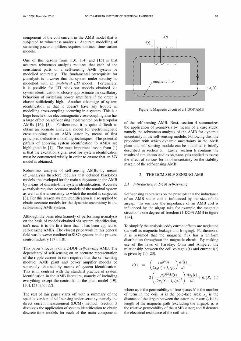
The characteristic parameters of the simulated AMB aresummarized in table 1 (some of which are explained infigure 2).
3. SYSTEM IDENTIFICATION OF THE NOMINALMODEL
Applying system identification to AMBs is a challengingexercise due to the inherent instability of magnetic
Table 1: Summary of the simulated self-sensing AMB
Parameter Value
KP (position PID controller) 20,000
KI (position PID controller) 700,000
KD (position PID controller) 38
KP (power amplifier PI controller) 0.7
KI (power amplifier PI controller) 0.01
Relative magnetic permeability 4,000
Power amplifier switching frequency 30 kHz
Supply voltage 50 V
Bias current 3 A
Resistance of coil wires 0.2 ΩCoil turns 50
Rotor mass 3.86 kg
Airgap 0.6 mm
Backup bearing inner radius 250 μmAxial bearing length 49.15 mm
Journal inner radius (rr) 15.88 mm
Journal outer radius(r j
)34.95 mm
Stator pole radius(rp
)35.60 mm
Stator back-iron inner radius (rc) 60.00 mm
Stator outer radius (rs) 75.00 mm
Pole width (rw) 13.89 mm
Figure 2: Physical dimensions of an AMB
bearings. Since open-loop operation of an AMB isimpossible, system identification must be performed whilethe AMB is in closed-loop operation. More details onclosed-loop system identification can be found in [27]and [1]. Other relevant system identification topics alsodiscussed in [1] include: the influence of the injectionpoint of the excitation signal; general parameterizedmodel structures suitable for AMBs and their associatedparameter estimation algorithms as well as the importanttopic of persistent excitation.
The main disadvantage of black-box modelling is that itgives limited insight into the internal dynamics of the realsystem. In the context of robustness analysis, this impliesthat it is difficult to apportion blame to specific systemcomponents when the total closed-loop system is fragile(and only a single model for the whole system is available).The solution to this problem is more detailed modellingwhere individual components in the control system are alsomodelled via system identification.
The main components in a 2-DOF self-sensing AMB
Vol.102(4) December 2011 SOUTH AFRICAN INSTITUTE OF ELECTRICAL ENGINEERS 101
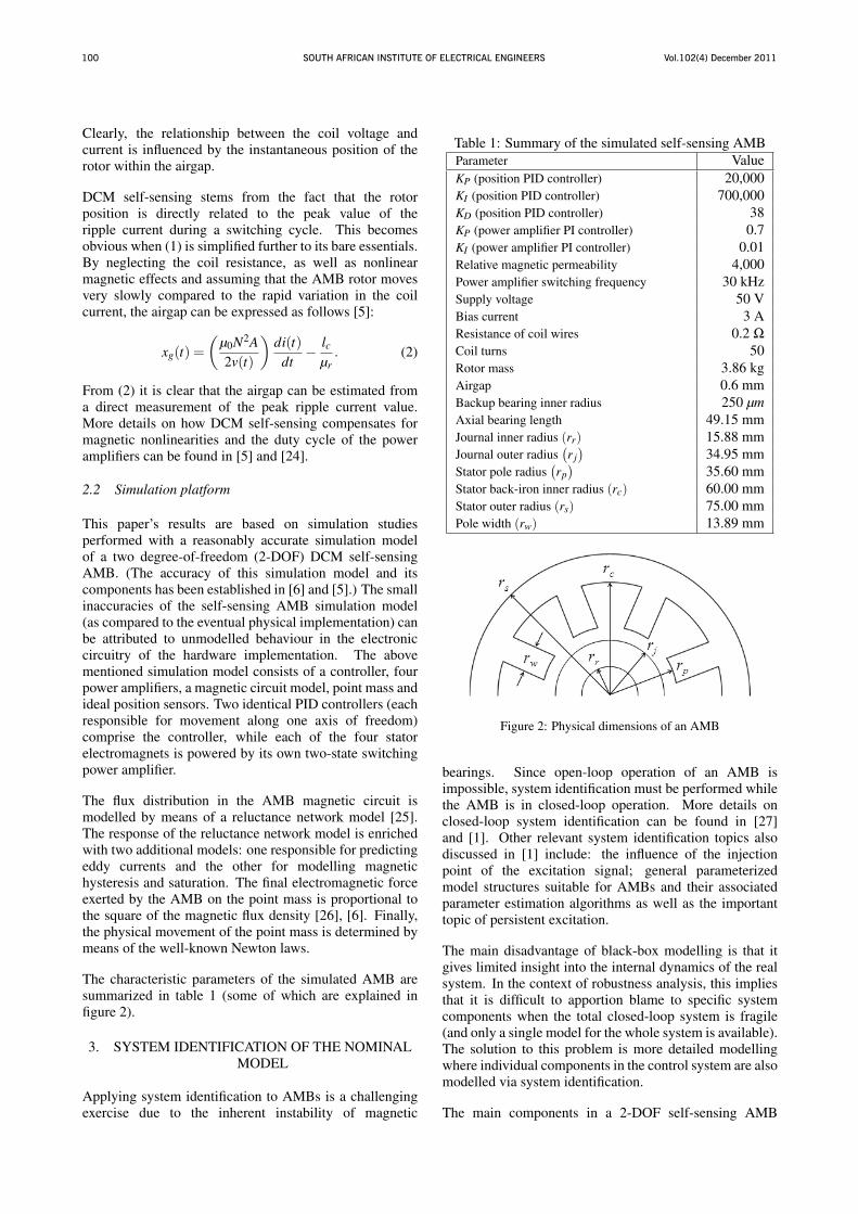
Figure 3: Block-diagram of an LTI self-sensing AMB
are the controller, power amplifiers, AMB plant andself-sensing module. A simplified block-diagram of a2-DOF self-sensing AMB is given in figure 3. In thisstudy the controller consists of two identical decoupledPID controllers, each responsible for the control of oneaxis of freedom.
The fundamental principle upon which self-sensing isbased is that the impedance of the coils (specifically theirinductance) is a function of the airgap [6]. This means thata power amplifier’s response is not only a function of thecontroller output, but also of the actual position of the masswithin the airgap. To ensure that the outputs of the LTIpower amplifier model contain position information, theLTI model should be an explicit function of all variablesthat have an effect on the real coil currents (namely twooutputs from the controller and two position signals fromthe output of the AMB plant).
The AMB model has four inputs (one for eachelectromagnet) and two outputs (namely the measuredx-axis and y-axis position of the rotor). In order to evaluatethe performance of the self-sensing algorithm, the x-axisrotor position is measured with an eddy-current positionsensor, while DCM self-sensing is only implemented onthe y-axis. DCM self-sensing (as implemented in [5]) onlytakes a single input (namely the current flowing in thetop pair of coils) to form an estimate of the y-axis rotorposition.
In contrast with the standard practice in the systemidentification literature, detrending is inadvisable whensystem identification is applied to self-sensing AMBs.This is because DCM self-sensing is sensitive for the biascurrent level in order to compensate for nonlinearity dueto hysteresis and saturation in the magnetic material ofthe AMB stator [5]. Detrending would therefore result inloss of information on the necessary setpoint of the LTIself-sensing model, with subsequent delevitation of therotor.
System identification works best if the sampling frequencyis commensurate with the time constants of the plant[28]. DCM self-sensing however requires accuratemeasurements of the peak values of the modulatedcomponent present at the switching frequency of the poweramplifiers (which is 30 kHz). This means that the eventualidentified models must have sampling frequencies higher
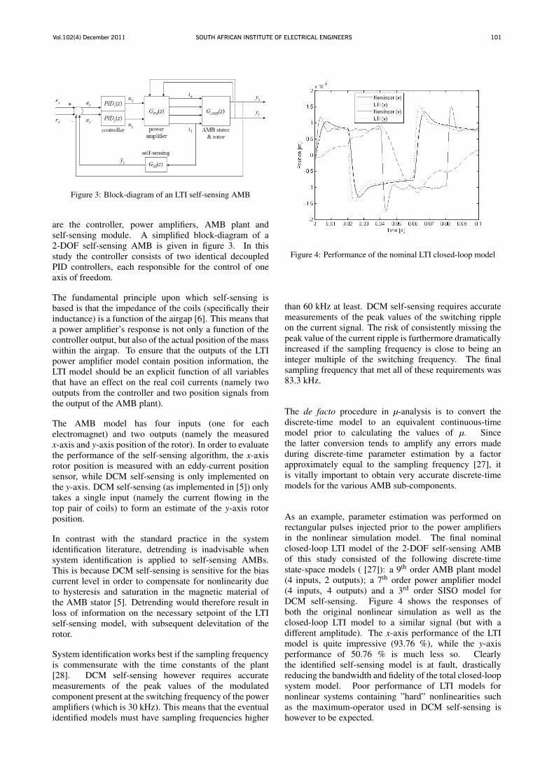
Figure 4: Performance of the nominal LTI closed-loop model
than 60 kHz at least. DCM self-sensing requires accuratemeasurements of the peak values of the switching rippleon the current signal. The risk of consistently missing thepeak value of the current ripple is furthermore dramaticallyincreased if the sampling frequency is close to being aninteger multiple of the switching frequency. The finalsampling frequency that met all of these requirements was83.3 kHz.
The de facto procedure in μ-analysis is to convert thediscrete-time model to an equivalent continuous-timemodel prior to calculating the values of μ. Sincethe latter conversion tends to amplify any errors madeduring discrete-time parameter estimation by a factorapproximately equal to the sampling frequency [27], itis vitally important to obtain very accurate discrete-timemodels for the various AMB sub-components.
As an example, parameter estimation was performed onrectangular pulses injected prior to the power amplifiersin the nonlinear simulation model. The final nominalclosed-loop LTI model of the 2-DOF self-sensing AMBof this study consisted of the following discrete-timestate-space models ( [27]): a 9th order AMB plant model(4 inputs, 2 outputs); a 7th order power amplifier model(4 inputs, 4 outputs) and a 3rd order SISO model forDCM self-sensing. Figure 4 shows the responses ofboth the original nonlinear simulation as well as theclosed-loop LTI model to a similar signal (but with adifferent amplitude). The x-axis performance of the LTImodel is quite impressive (93.76 %), while the y-axisperformance of 50.76 % is much less so. Clearlythe identified self-sensing model is at fault, drasticallyreducing the bandwidth and fidelity of the total closed-loopsystem model. Poor performance of LTI models fornonlinear systems containing ”hard” nonlinearities suchas the maximum-operator used in DCM self-sensing ishowever to be expected.
Vol.102(4) December 2011SOUTH AFRICAN INSTITUTE OF ELECTRICAL ENGINEERS102
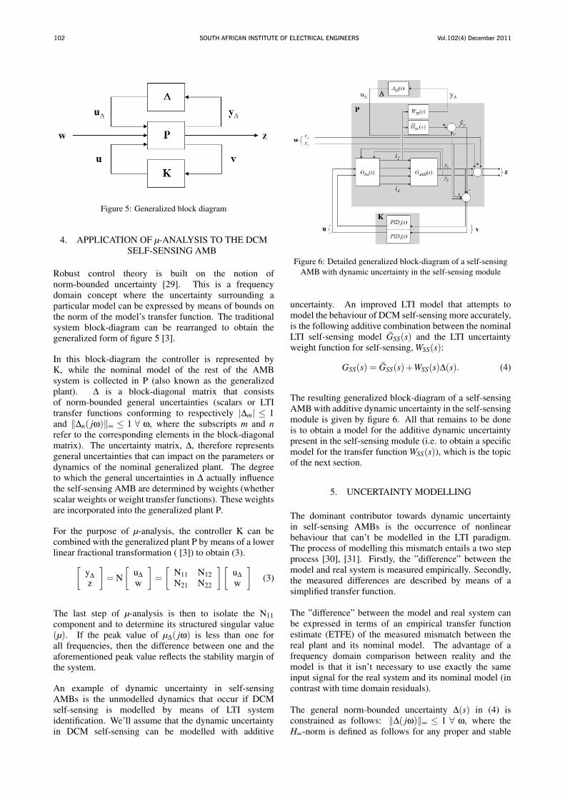
Figure 5: Generalized block diagram
4. APPLICATION OF μ-ANALYSIS TO THE DCMSELF-SENSING AMB
Robust control theory is built on the notion ofnorm-bounded uncertainty [29]. This is a frequencydomain concept where the uncertainty surrounding aparticular model can be expressed by means of bounds onthe norm of the model’s transfer function. The traditionalsystem block-diagram can be rearranged to obtain thegeneralized form of figure 5 [3].
In this block-diagram the controller is represented byK, while the nominal model of the rest of the AMBsystem is collected in P (also known as the generalizedplant). Δ is a block-diagonal matrix that consistsof norm-bounded general uncertainties (scalars or LTItransfer functions conforming to respectively |Δm| ≤ 1and ‖Δn( jω)‖∞ ≤ 1 ∀ ω, where the subscripts m and nrefer to the corresponding elements in the block-diagonalmatrix). The uncertainty matrix, Δ, therefore representsgeneral uncertainties that can impact on the parameters ordynamics of the nominal generalized plant. The degreeto which the general uncertainties in Δ actually influencethe self-sensing AMB are determined by weights (whetherscalar weights or weight transfer functions). These weightsare incorporated into the generalized plant P.
For the purpose of μ-analysis, the controller K can becombined with the generalized plant P by means of a lowerlinear fractional transformation ( [3]) to obtain (3).[
yΔz
]= N
[uΔw
]=
[N11 N12
N21 N22
][uΔw
](3)
The last step of μ-analysis is then to isolate the N11
component and to determine its structured singular value(μ). If the peak value of μΔ( jω) is less than one forall frequencies, then the difference between one and theaforementioned peak value reflects the stability margin ofthe system.
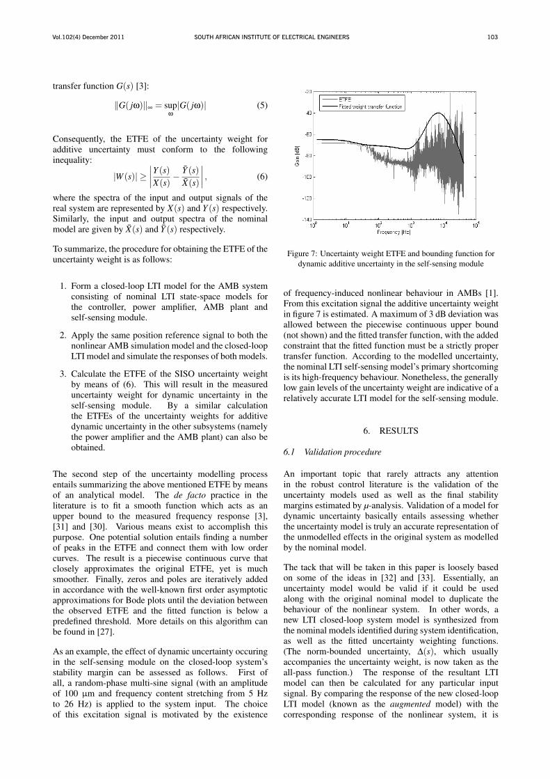
An example of dynamic uncertainty in self-sensingAMBs is the unmodelled dynamics that occur if DCMself-sensing is modelled by means of LTI systemidentification. We’ll assume that the dynamic uncertaintyin DCM self-sensing can be modelled with additive
Figure 6: Detailed generalized block-diagram of a self-sensing
AMB with dynamic uncertainty in the self-sensing module
uncertainty. An improved LTI model that attempts tomodel the behaviour of DCM self-sensing more accurately,is the following additive combination between the nominalLTI self-sensing model GSS(s) and the LTI uncertaintyweight function for self-sensing, WSS(s):
GSS(s) = GSS(s)+WSS(s)Δ(s). (4)
The resulting generalized block-diagram of a self-sensingAMB with additive dynamic uncertainty in the self-sensingmodule is given by figure 6. All that remains to be doneis to obtain a model for the additive dynamic uncertaintypresent in the self-sensing module (i.e. to obtain a specificmodel for the transfer function WSS(s)), which is the topicof the next section.
5. UNCERTAINTY MODELLING
The dominant contributor towards dynamic uncertaintyin self-sensing AMBs is the occurrence of nonlinearbehaviour that can’t be modelled in the LTI paradigm.The process of modelling this mismatch entails a two stepprocess [30], [31]. Firstly, the ”difference” between themodel and real system is measured empirically. Secondly,the measured differences are described by means of asimplified transfer function.
The ”difference” between the model and real system canbe expressed in terms of an empirical transfer functionestimate (ETFE) of the measured mismatch between thereal plant and its nominal model. The advantage of afrequency domain comparison between reality and themodel is that it isn’t necessary to use exactly the sameinput signal for the real system and its nominal model (incontrast with time domain residuals).
The general norm-bounded uncertainty Δ(s) in (4) isconstrained as follows: ‖Δ( jω)‖∞ ≤ 1 ∀ ω, where theH∞-norm is defined as follows for any proper and stable
Vol.102(4) December 2011 SOUTH AFRICAN INSTITUTE OF ELECTRICAL ENGINEERS 103
transfer function G(s) [3]:
‖G( jω)‖∞ = supω|G( jω)| (5)
Consequently, the ETFE of the uncertainty weight foradditive uncertainty must conform to the followinginequality:
|W (s)| ≥∣∣∣∣Y (s)X(s)
− Y (s)X(s)
∣∣∣∣ , (6)
where the spectra of the input and output signals of thereal system are represented by X(s) and Y (s) respectively.Similarly, the input and output spectra of the nominalmodel are given by X(s) and Y (s) respectively.
To summarize, the procedure for obtaining the ETFE of theuncertainty weight is as follows:
1. Form a closed-loop LTI model for the AMB systemconsisting of nominal LTI state-space models forthe controller, power amplifier, AMB plant andself-sensing module.
2. Apply the same position reference signal to both thenonlinear AMB simulation model and the closed-loopLTI model and simulate the responses of both models.
3. Calculate the ETFE of the SISO uncertainty weightby means of (6). This will result in the measureduncertainty weight for dynamic uncertainty in theself-sensing module. By a similar calculationthe ETFEs of the uncertainty weights for additivedynamic uncertainty in the other subsystems (namelythe power amplifier and the AMB plant) can also beobtained.
The second step of the uncertainty modelling processentails summarizing the above mentioned ETFE by meansof an analytical model. The de facto practice in theliterature is to fit a smooth function which acts as anupper bound to the measured frequency response [3],[31] and [30]. Various means exist to accomplish thispurpose. One potential solution entails finding a numberof peaks in the ETFE and connect them with low ordercurves. The result is a piecewise continuous curve thatclosely approximates the original ETFE, yet is muchsmoother. Finally, zeros and poles are iteratively addedin accordance with the well-known first order asymptoticapproximations for Bode plots until the deviation betweenthe observed ETFE and the fitted function is below apredefined threshold. More details on this algorithm canbe found in [27].
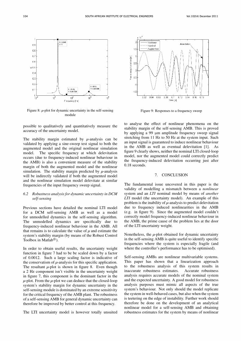
As an example, the effect of dynamic uncertainty occuringin the self-sensing module on the closed-loop system’sstability margin can be assessed as follows. First ofall, a random-phase multi-sine signal (with an amplitudeof 100 μm and frequency content stretching from 5 Hzto 26 Hz) is applied to the system input. The choiceof this excitation signal is motivated by the existence
Figure 7: Uncertainty weight ETFE and bounding function for
dynamic additive uncertainty in the self-sensing module
of frequency-induced nonlinear behaviour in AMBs [1].From this excitation signal the additive uncertainty weightin figure 7 is estimated. A maximum of 3 dB deviation wasallowed between the piecewise continuous upper bound(not shown) and the fitted transfer function, with the addedconstraint that the fitted function must be a strictly propertransfer function. According to the modelled uncertainty,the nominal LTI self-sensing model’s primary shortcomingis its high-frequency behaviour. Nonetheless, the generallylow gain levels of the uncertainty weight are indicative of arelatively accurate LTI model for the self-sensing module.
6. RESULTS
6.1 Validation procedure
An important topic that rarely attracts any attentionin the robust control literature is the validation of theuncertainty models used as well as the final stabilitymargins estimated by μ-analysis. Validation of a model fordynamic uncertainty basically entails assessing whetherthe uncertainty model is truly an accurate representation ofthe unmodelled effects in the original system as modelledby the nominal model.
The tack that will be taken in this paper is loosely basedon some of the ideas in [32] and [33]. Essentially, anuncertainty model would be valid if it could be usedalong with the original nominal model to duplicate thebehaviour of the nonlinear system. In other words, anew LTI closed-loop system model is synthesized fromthe nominal models identified during system identification,as well as the fitted uncertainty weighting functions.(The norm-bounded uncertainty, Δ(s), which usuallyaccompanies the uncertainty weight, is now taken as theall-pass function.) The response of the resultant LTImodel can then be calculated for any particular inputsignal. By comparing the response of the new closed-loopLTI model (known as the augmented model) with thecorresponding response of the nonlinear system, it is
Vol.102(4) December 2011SOUTH AFRICAN INSTITUTE OF ELECTRICAL ENGINEERS104
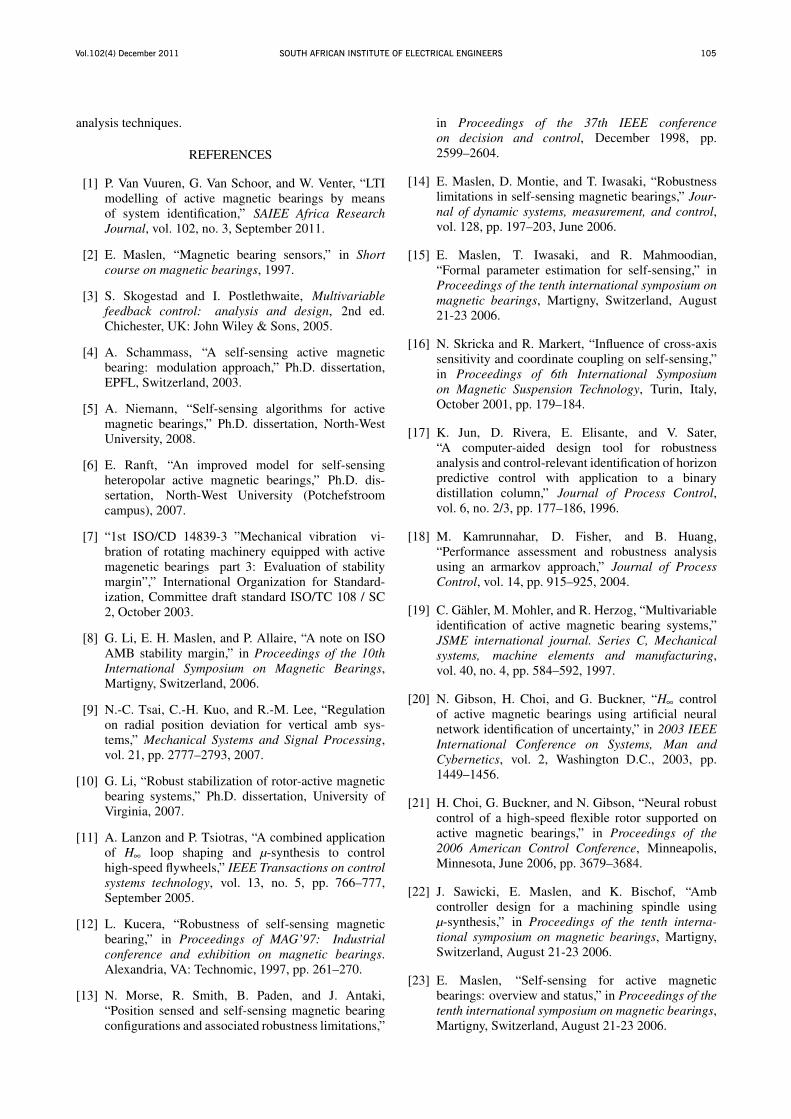
Figure 8: μ-plot for dynamic uncertainty in the self-sensing
module
possible to qualitatively and quantitatively measure theaccuracy of the uncertainty model.
The stability margin estimated by μ-analysis can bevaldated by applying a sine-sweep test signal to both theaugmented model and the original nonlinear simulationmodel. The specific frequency at which delevitationoccurs (due to frequency-induced nonlinear behaviour inthe AMB) is also a convenient measure of the stabilitymargin of both the augmented model and the nonlinearsimulation. The stability margin predicted by μ-analysiswill be indirectly validated if both the augmented modeland the nonlinear simulation model delevitate at similarfrequencies of the input frequency sweep signal.
6.2 Robustness analysis for dynamic uncertainty in DCMself-sensing
Previous sections have detailed the nominal LTI modelfor a DCM self-sensing AMB as well as a modelfor unmodelled dynamics in the self-sensing algorithm.The unmodelled dynamics are specifically due tofrequency-induced nonlinear behaviour in the AMB. Allthat remains is to calculate the value of μ and estimate thesystem’s stability margin (by means of the Robust ControlToolbox in Matlab�).
In order to obtain useful results, the uncertainty weightfunction in figure 7 had to be be scaled down by a factorof 0.0012. Such a large scaling factor is indicative ofthe conservatism of μ-analysis for this specific application.The resultant μ-plot is shown in figure 8. Even thougha 2 Hz component isn’t visible in the uncertainty weightin figure 7, this component is the dominant factor in theμ-plot. From the μ-plot we can deduce that the closed-loopsystem’s stability margin for dynamic uncertainty in theself-sensing module is dominated by an extreme sensitivityfor the critical frequency of the AMB plant. The robustnessof a self-sensing AMB for general dynamic uncertainty cantherefore be improved by better control at this frequency.
The LTI uncertainty model is however totally unsuited
Figure 9: Responses to a frequency sweep
to analyse the effect of nonlinear phenomena on thestability margin of the self-sensing AMB. This is provedby applying a 99 μm amplitude frequency sweep signalstretching from 11 Hz to 50 Hz at the system input. Suchan input signal is guaranteed to induce nonlinear behaviourin the AMB as well as eventual delevitation [1]. Asfigure 9 clearly shows, neither the nominal LTI closed-loopmodel, nor the augmented model could correctly predictthe frequency-induced delevitation occurring just after0.18 seconds.
7. CONCLUSION
The fundamental issue uncovered in this paper is thevalidity of modelling a mismatch between a nonlinearsystem and an LTI nominal model by means of anotherLTI model (the uncertainty model). An example of thisproblem is the inability of μ-analysis to predict delevitationdue to frequency induced nonlinearities in the AMB(e.g. in figure 9). Since the augmented model couldn’tcorrectly model frequency-induced nonlinear behaviour inthe AMB, the prime cause of the problem lies at the doorof the LTI uncertainty weight.
Nonetheless, the μ-plot obtained for dynamic uncertaintyin the self-sensing AMB is quite useful to identify specificfrequencies where the system is especially fragile (andwhere the controller’s performance has to be optimised).
Self-sensing AMBs are nonlinear multivariable systems.This paper has shown that a linearization approachto the robustness analysis of this system results ininaccurate robustness estimates. Accurate robustnessanalysis requires accurate models of the nominal systemand the expected uncertainty. A good model for robustnessanalysis purposes must mimic all aspects of the truesystem’s behaviour. Not only should the model replicatethe system in well-behaved cases, but also when the systemis teetering on the edge of instability. Further work shouldtherefore be done on the development of an analyticalnonlinear model for a self-sensing AMB and obtainingrobustness estimates for the system by means of nonlinear
Vol.102(4) December 2011 SOUTH AFRICAN INSTITUTE OF ELECTRICAL ENGINEERS 105
analysis techniques.
REFERENCES
[1] P. Van Vuuren, G. Van Schoor, and W. Venter, “LTImodelling of active magnetic bearings by meansof system identification,” SAIEE Africa ResearchJournal, vol. 102, no. 3, September 2011.
[2] E. Maslen, “Magnetic bearing sensors,” in Shortcourse on magnetic bearings, 1997.
[3] S. Skogestad and I. Postlethwaite, Multivariablefeedback control: analysis and design, 2nd ed.Chichester, UK: John Wiley & Sons, 2005.
[4] A. Schammass, “A self-sensing active magneticbearing: modulation approach,” Ph.D. dissertation,EPFL, Switzerland, 2003.
[5] A. Niemann, “Self-sensing algorithms for activemagnetic bearings,” Ph.D. dissertation, North-WestUniversity, 2008.
[6] E. Ranft, “An improved model for self-sensingheteropolar active magnetic bearings,” Ph.D. dis-sertation, North-West University (Potchefstroomcampus), 2007.
[7] “1st ISO/CD 14839-3 ”Mechanical vibration vi-bration of rotating machinery equipped with activemagenetic bearings part 3: Evaluation of stabilitymargin”,” International Organization for Standard-ization, Committee draft standard ISO/TC 108 / SC2, October 2003.
[8] G. Li, E. H. Maslen, and P. Allaire, “A note on ISOAMB stability margin,” in Proceedings of the 10thInternational Symposium on Magnetic Bearings,Martigny, Switzerland, 2006.
[9] N.-C. Tsai, C.-H. Kuo, and R.-M. Lee, “Regulationon radial position deviation for vertical amb sys-tems,” Mechanical Systems and Signal Processing,vol. 21, pp. 2777–2793, 2007.
[10] G. Li, “Robust stabilization of rotor-active magneticbearing systems,” Ph.D. dissertation, University ofVirginia, 2007.
[11] A. Lanzon and P. Tsiotras, “A combined applicationof H∞ loop shaping and μ-synthesis to controlhigh-speed flywheels,” IEEE Transactions on controlsystems technology, vol. 13, no. 5, pp. 766–777,September 2005.
[12] L. Kucera, “Robustness of self-sensing magneticbearing,” in Proceedings of MAG’97: Industrialconference and exhibition on magnetic bearings.Alexandria, VA: Technomic, 1997, pp. 261–270.
[13] N. Morse, R. Smith, B. Paden, and J. Antaki,“Position sensed and self-sensing magnetic bearingconfigurations and associated robustness limitations,”
in Proceedings of the 37th IEEE conferenceon decision and control, December 1998, pp.2599–2604.
[14] E. Maslen, D. Montie, and T. Iwasaki, “Robustnesslimitations in self-sensing magnetic bearings,” Jour-nal of dynamic systems, measurement, and control,vol. 128, pp. 197–203, June 2006.
[15] E. Maslen, T. Iwasaki, and R. Mahmoodian,“Formal parameter estimation for self-sensing,” inProceedings of the tenth international symposium onmagnetic bearings, Martigny, Switzerland, August21-23 2006.
[16] N. Skricka and R. Markert, “Influence of cross-axissensitivity and coordinate coupling on self-sensing,”in Proceedings of 6th International Symposiumon Magnetic Suspension Technology, Turin, Italy,October 2001, pp. 179–184.
[17] K. Jun, D. Rivera, E. Elisante, and V. Sater,“A computer-aided design tool for robustnessanalysis and control-relevant identification of horizonpredictive control with application to a binarydistillation column,” Journal of Process Control,vol. 6, no. 2/3, pp. 177–186, 1996.
[18] M. Kamrunnahar, D. Fisher, and B. Huang,“Performance assessment and robustness analysisusing an armarkov approach,” Journal of ProcessControl, vol. 14, pp. 915–925, 2004.
[19] C. Gahler, M. Mohler, and R. Herzog, “Multivariableidentification of active magnetic bearing systems,”JSME international journal. Series C, Mechanicalsystems, machine elements and manufacturing,vol. 40, no. 4, pp. 584–592, 1997.
[20] N. Gibson, H. Choi, and G. Buckner, “H∞ controlof active magnetic bearings using artificial neuralnetwork identification of uncertainty,” in 2003 IEEEInternational Conference on Systems, Man andCybernetics, vol. 2, Washington D.C., 2003, pp.1449–1456.
[21] H. Choi, G. Buckner, and N. Gibson, “Neural robustcontrol of a high-speed flexible rotor supported onactive magnetic bearings,” in Proceedings of the2006 American Control Conference, Minneapolis,Minnesota, June 2006, pp. 3679–3684.
[22] J. Sawicki, E. Maslen, and K. Bischof, “Ambcontroller design for a machining spindle usingμ-synthesis,” in Proceedings of the tenth interna-tional symposium on magnetic bearings, Martigny,Switzerland, August 21-23 2006.
[23] E. Maslen, “Self-sensing for active magneticbearings: overview and status,” in Proceedings of thetenth international symposium on magnetic bearings,Martigny, Switzerland, August 21-23 2006.
Vol.102(4) December 2011SOUTH AFRICAN INSTITUTE OF ELECTRICAL ENGINEERS106
[24] A. Niemann and G. Van Schoor, “Self-sensingalgorithm for active magnetic bearings; using directcurrent measurements,” in Proceedings of the 12thInternational Symposium on Magnetic Bearings.Wuhan, China: ISMB, August 2010.
[25] D. Meeker, E. Maslen, and M. Noh, “An augmentedcircuit model for magnetic bearings including eddycurrents, fringing, and leakage,” IEEE Transactionson Magnetics, vol. 32, no. 4, pp. 3219–3227, July1996.
[26] G. Schweitzer, H. Bleuler, and A. Traxler, ActiveMagnetic Bearings: Basics, Properties and Applica-tions of Active Magnetic Bearings. Zurich: AuthorsReprint, 2003.
[27] P. Van Vuuren, “Robustness estimation ofself-sensing active magnetic bearings via systemidentification,” Ph.D. dissertation, North-WestUniversity, 2010.
[28] L. Ljung, System identification: theory for the user,2nd ed. Upper Saddle River, NJ: Prentice Hall, 1999.
[29] K. Zhou, J. Doyle, and K. Glover, Robust and optimalcontrol. Upper Saddle River, NJ: Prentice Hall,1996.
[30] D. Bayard, Y. Yam, and E. Mettler, “A criterionfor joint optimization of identification and robustcontrol,” IEEE Transactions on Automatic Control,vol. 37, no. 7, pp. 986–991, July 1992.
[31] B. Lu, H. Choi, G. Buckner, and K. Tammi,“Linear parameter-varying techniques for control ofa magnetic bearing system,” Control EngineeringPractice, vol. 16, pp. 1161–1172, 2008.
[32] R. Smith, “Model validation for robust control: anexperimental process control application,” Automat-ica, vol. 31, no. 11, pp. 1637–1647, 1995.
[33] H. Buckner, G.D. Choi and N. Gibson, “Estimatingmodel uncertainty using confidence interval net-works: applications to robust control,” Transactionsof the ASME: Journal of dynamic systems, measure-ment, and control, vol. 128, pp. 626–635, September2006.
Vol.102(4) December 2011 SOUTH AFRICAN INSTITUTE OF ELECTRICAL ENGINEERS 107
MODELLING OF BROADBAND POWERLINE COMMUNICATION CHANNELS C.T. Mulangu, T.J. Afullo and N.M. Ijumba School of Electrical, Electronic and Computer Engineering, University of KwaZulu-Natal, Private Bag X54001, Durban 4000, South Africa E-mail: [email protected]; [email protected]; [email protected] Abstract: This paper develops a new PLC model and investigates the impact of the load, line length, and diameter of the transmission line on the channel transfer function over the frequency range of 1-20 MHz. The results show that with 42 degrees of freedom, the proposed model leads to an average RMSE value of approximately 5.2 dB. With the same conditions, the Phillips model leads to an average RMSE value of approximately 1.62 dB. Keywords: Power Line Telecommunication, PLC Channel Transfer function, Broadband PLC
1. INTRODUCTION
Considerable effort has been recently devoted to the determination of accurate channel models for the Power Line Communication (PLC) environment, both for indoor and outdoor cases. Power lines have been used as a communication medium for many years in low bit-rate applications like automation of power distribution and remote meter reading [1-2]. However, the characterization of the transfer function is a non-trivial task to achieve since PLC characteristics change depending on the particular topology of a given link. The attenuation depends much more on network topology and connected loads. The amplitude characteristics show, even at short distances, deep narrowband notches of high attenuation, which can even be higher than those for longer distances. These notches result from reflections and multipath propagation. This behaviour is very similar to the one of mobile radio channels. The conversion of networks designed to distribute electric power into communication media has been the subject of extensive research carried out over the last few years. The growing demand for information exchange calls for high rate data transmission, which in turn requires the utilization of the power grid in the frequency range up to 30 MHz. Several problems are caused by the frequency-dependent nature of the power grid, the presence of time varying loads, as well as by the structure of the grid itself. The solutions for these problems can be achieved through proper modelling of the power grid as a communication medium with a time-varying delay. Several channel models from multipath propagation principles have been proposed [3], [4], [5]. The works presented in [4] and [6] are very close to the approach introduced herein. Models proposed in the literature focus on the subject of in-home networks, i.e. the power distribution networks inside consumer premises. In this paper, the model parameters are derived from the lumped-circuit transmission line model to obtain the
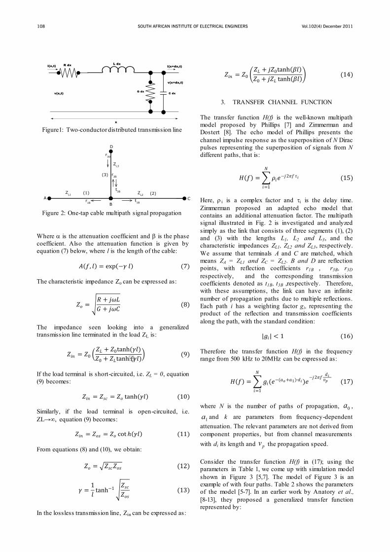
transfer function of the channel, as shown in Fig.1, using equations (1) and (2) below:
In these equations x denotes the longitudinal direction of the line, while R, L, G and C are the per-unit length resistance (Ω/m), inductance (H/m), conductance (S/m) and capacitance (F/m), respectively.
2. TRANSMISSION LINE PARAMETERS
Anatory et al., [7], have defined the transmission parameters for the PLC system from a primary substation to the customer bracket. They assumed that the separation distance D, between conductors is much greater than the radius, a of the conductors; hence the capacitance C, inductance L, and AC resistance R per loop meter are given by [1], [2]:
Here and are the permeability and conductivity of the metal conductors, respectively. The propagation coefficient is given by:
Vol.102(4) December 2011SOUTH AFRICAN INSTITUTE OF ELECTRICAL ENGINEERS108
Where is the attenuation coefficient and is the phase coefficient. Also the attenuation function is given by equation (7) below, where l is the length of the cable:
The characteristic impedance Zo can be expressed as:
The impedance seen looking into a generalized transmission line terminated in the load ZL is:
If the load terminal is short-circuited, i.e. ZL = 0, equation (9) becomes:
Similarly, if the load terminal is open-circuited, i.e. ZL→∞, equation (9) becomes:
From equations (8) and (10), we obtain:
In the lossless transmission line, Zin can be expressed as:
3. TRANSFER CHANNEL FUNCTION The transfer function H(f) is the well-known multipath model proposed by Phillips [7] and Zimmerman and Dostert [8]. The echo model of Phillips presents the channel impulse response as the superposition of N Dirac pulses representing the superposition of signals from N different paths, that is:
Here, i is a complex factor and i is the delay time. Zimmerman proposed an adapted echo model that contains an additional attenuation factor. The multipath signal illustrated in Fig. 2 is investigated and analyzed simply as the link that consists of three segments (1), (2) and (3) with the lengths L1, L2 and L3, and the characteristic impedances ZL1, ZL2 and ZL3, respectively. We assume that terminals A and C are matched, which means ZA = ZL1 and ZC = ZL2. B and D are reflection points, with reflection coefficients r1B , r3B, r3D respectively, and the corresponding transmission coefficients denoted as t1B, t3B ,respectively. Therefore, with these assumptions, the link can have an infinite number of propagation paths due to multiple reflections. Each path i has a weighting factor gi, representing the product of the reflection and transmission coefficients along the path, with the standard condition:
Therefore the transfer function H(f) in the frequency range from 500 kHz to 20MHz can be expressed as:
where N is the number of paths of propagation, 0a ,
1a and k are parameters from frequency-dependent attenuation. The relevant parameters are not derived from component properties, but from channel measurements with di its length and pv
the propagation speed.
Consider the transfer function H(f) in (17); using the parameters in Table 1, we come up with simulation model shown in Figure 3 [5,7]. The model of Figure 3 is an example of with four paths. Table 2 shows the parameters of the model [5-7]. In an earlier work by Anatory et al., [8-13], they proposed a generalized transfer function represented by:
Figure1: Two-conductor distributed transmission line
Figure 2: One-tap cable multipath signal propagation
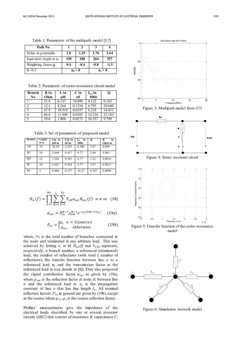
Vol.102(4) December 2011 SOUTH AFRICAN INSTITUTE OF ELECTRICAL ENGINEERS 109
where, NT is the total number of branches connected at the node and terminated in any arbitrary load. This was achieved by letting n, m M, Hmn(f) and TLM, represent, respectively, a branch number, a referenced (terminated) load, the number of reflections (with total L number of reflections), the transfer function between line n to a referenced load m, and the transmission factor at the referenced load m (see details in [8]). They also proposed the signal contribution factor mn as given by (19a), where nm is the reflection factor at node B, between line n and the referenced load m. γn is the propagation constant of line n that has line length ln. All terminal reflection factors PLn in general are given by (19b), except at the source where L1= s is the source reflection factor. Phillips’ measurements give the impedance of the electrical loads described by one or several resonant circuits (SRC) that consist of resistance R, capacitance C,
Table 1: Parameters of the multipath model [5,7]
Path No 1 2 3 4 Delay in μ-seconds 1.0 1.25 1.76 2.64 Equivalent length in m 150 188 264 397 Weighting factor gi 0.4 -0.4 -0.8 -1.5 K=0.5 a0 = 0 a1 = 0
Table 2: Parameters of series-resonance circuit model
Branch No
R in Ohm
L in μH
C in nF
fres in MHz
Q
1 21.4 0.137 10.890 4.122 0.165 2 12.1 8.264 0.1334 4.793 20.640 3 67.9 18.919 0.0197 8.238 14.431 4 46.4 11.948 0.0103 14.324 23.183 5 19.6 1.008 0.0273 30.357 9.799
Table 3: Set of parameters of proposed model Branch Length
in m Lm in μH/m
Cm in nF/m
f m in MHz
Q R in Ohm/m
AB 70 20.69 2.635 0.596 3.67 0.008
BC 10 2.668 0.417 4.77 2.04 0.001
BD 12 3.201 0.501 4.77 1.22 0.0016
BF 10 2.667 0.418 4.77 3.67 0.0013
BE 3 0.880 0.137 14.37 9.767 0.0004
1 5 10 15 20-60
-40
-20
0
Frequency/MHz
|H(f)
|/dB
Simulation with N=4 Paths
Figure 3: Multipath model from (17)
Figure 4: Series resonant circuit
0 0.5 1 1.5 2 2.5 3
x 107
-35
-30
-25
-20
-15
-10
Frequency in Hz
Mag
nitu
de o
f Tra
nsfe
r Fun
ctio
n
Figure 5: Transfer function of the series resonance
model
Figure 6: Simulation network model
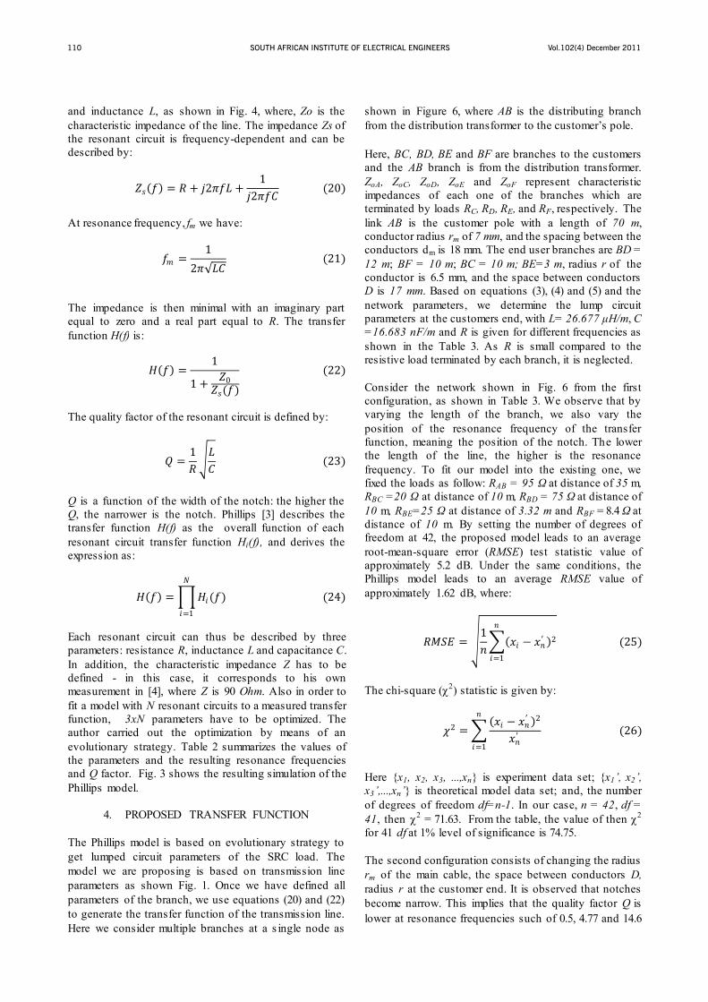
Vol.102(4) December 2011SOUTH AFRICAN INSTITUTE OF ELECTRICAL ENGINEERS110
and inductance L, as shown in Fig. 4, where, Zo is the characteristic impedance of the line. The impedance Zs of the resonant circuit is frequency-dependent and can be described by:
At resonance frequency, fm we have:
The impedance is then minimal with an imaginary part equal to zero and a real part equal to R. The transfer function H(f) is:
The quality factor of the resonant circuit is defined by:
Q is a function of the width of the notch: the higher the Q, the narrower is the notch. Phillips [3] describes the transfer function H(f) as the overall function of each resonant circuit transfer function Hi(f), and derives the expression as:
Each resonant circuit can thus be described by three parameters: resistance R, inductance L and capacitance C. In addition, the characteristic impedance Z has to be defined - in this case, it corresponds to his own measurement in [4], where Z is 90 Ohm. Also in order to fit a model with N resonant circuits to a measured transfer function, 3xN parameters have to be optimized. The author carried out the optimization by means of an evolutionary strategy. Table 2 summarizes the values of the parameters and the resulting resonance frequencies and Q factor. Fig. 3 shows the resulting simulation of the Phillips model.
4. PROPOSED TRANSFER FUNCTION The Phillips model is based on evolutionary strategy to get lumped circuit parameters of the SRC load. The model we are proposing is based on transmission line parameters as shown Fig. 1. Once we have defined all parameters of the branch, we use equations (20) and (22) to generate the transfer function of the transmission line. Here we consider multiple branches at a s ingle node as
shown in Figure 6, where AB is the distributing branch from the distribution transformer to the customer’s pole. Here, BC, BD, BE and BF are branches to the customers and the AB branch is from the distribution transformer. ZoA, ZoC, ZoD, ZoE and ZoF represent characteristic impedances of each one of the branches which are terminated by loads RC, RD, RE, and RF, respectively. The link AB is the customer pole with a length of 70 m, conductor radius rm of 7 mm, and the spacing between the conductors dm is 18 mm. The end user branches are BD = 12 m; BF = 10 m; BC = 10 m; BE=3 m, radius r of the conductor is 6.5 mm, and the space between conductors D is 17 mm. Based on equations (3), (4) and (5) and the network parameters, we determine the lump circuit parameters at the customers end, with L= 26.677 μH/m, C =16.683 nF/m and R is given for different frequencies as shown in the Table 3. As R is small compared to the resistive load terminated by each branch, it is neglected. Consider the network shown in Fig. 6 from the first configuration, as shown in Table 3. We observe that by varying the length of the branch, we also vary the position of the resonance frequency of the transfer function, meaning the position of the notch. The lower the length of the line, the higher is the resonance frequency. To fit our model into the existing one, we fixed the loads as follow: RAB = 95 Ω at distance of 35 m, RBC =20 Ω at distance of 10 m, RBD = 75 Ω at distance of 10 m, RBE=25 Ω at distance of 3.32 m and RBF = 8.4 Ω at distance of 10 m. By setting the number of degrees of freedom at 42, the proposed model leads to an average root-mean-square error (RMSE) test statistic value of approximately 5.2 dB. Under the same conditions, the Phillips model leads to an average RMSE value of approximately 1.62 dB, where:
The chi-square ( 2) statistic is given by:
Here {x1, x2, x3, ...,xn} is experiment data set; {x1’, x2’, x3’,...,xn’} is theoretical model data set; and, the number of degrees of freedom df=n-1. In our case, n = 42, df = 41, then 2 = 71.63. From the table, the value of then 2 for 41 df at 1% level of significance is 74.75. The second configuration consists of changing the radius rm of the main cable, the space between conductors D, radius r at the customer end. It is observed that notches become narrow. This implies that the quality factor Q is lower at resonance frequencies such of 0.5, 4.77 and 14.6
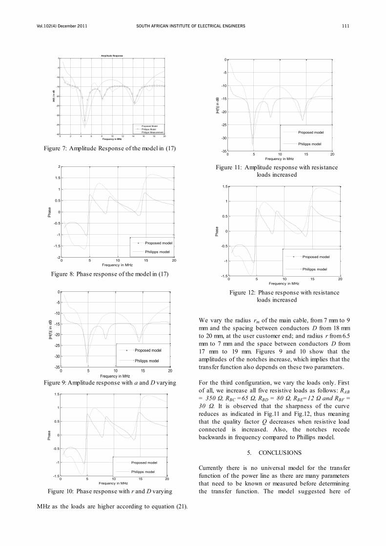
Vol.102(4) December 2011 SOUTH AFRICAN INSTITUTE OF ELECTRICAL ENGINEERS 111
MHz as the loads are higher according to equation (21).
We vary the radius rm of the main cable, from 7 mm to 9 mm and the spacing between conductors D from 18 mm to 20 mm, at the user customer end; and radius r from 6.5 mm to 7 mm and the space between conductors D from 17 mm to 19 mm. Figures 9 and 10 show that the amplitudes of the notches increase, which implies that the transfer function also depends on these two parameters. For the third configuration, we vary the loads only. First of all, we increase all five resistive loads as follows: RAB = 350 Ω, RBC =65 Ω, RBD = 80 Ω, RBE=12 Ω and RBF = 30 Ω. It is observed that the sharpness of the curve reduces as indicated in Fig.11 and Fig.12, thus meaning that the quality factor Q decreases when resistive load connected is increased. Also, the notches recede backwards in frequency compared to Phillips model.
5. CONCLUSIONS Currently there is no universal model for the transfer function of the power line as there are many parameters that need to be known or measured before determining the transfer function. The model suggested here of
0 2 4 6 8 10 12 14 16 18 20-40
-35
-30
-25
-20
-15
-10
-5
0Amplitude Response
Frequency in MHz
|H(f)
| in
dB
Proposed ModelPhilipps ModelPhilipps Measurement
Figure 7: Amplitude Response of the model in (17)
0 5 10 15 20-2
-1.5
-1
-0.5
0
0.5
1
1.5
2
Frequency in MHz
Phas
e
Proposed model
Philipps model
Figure 8: Phase response of the model in (17)
0 5 10 15 20-35
-30
-25
-20
-15
-10
-5
0
Frequency in MHz
|H(f
)| in
dB
Proposed model
Philipps model
Figure 9: Amplitude response with a and D varying
0 5 10 15 20-1.5
-1
-0.5
0
0.5
1
1.5
Frequency in MHz
Phas
e
Proposed model
Philipps model
Figure 10: Phase response with r and D varying
0 5 10 15 20-35
-30
-25
-20
-15
-10
-5
0
Frequency in MHz
|H(f)
| in
dB
Proposed model
Philipps model
Figure 11: Amplitude response with resistance loads increased
0 5 10 15 20-1.5
-1
-0.5
0
0.5
1
1.5
Frequency in MHz
Phas
e
Proposed model
Philipps model
Figure 12: Phase response with resistance loads increased
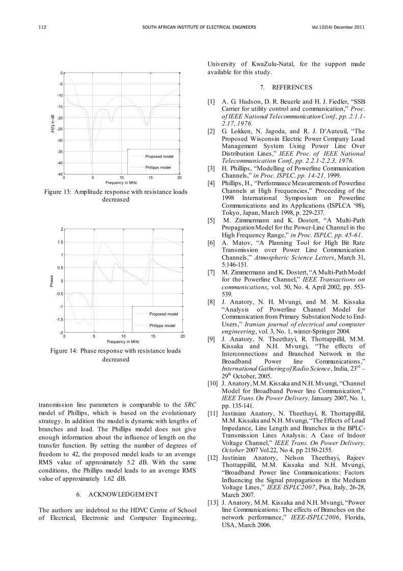
Vol.102(4) December 2011SOUTH AFRICAN INSTITUTE OF ELECTRICAL ENGINEERS112
transmission line parameters is comparable to the SRC model of Phillips, which is based on the evolutionary strategy. In addition the model is dynamic with lengths of branches and load. The Phillips model does not give enough information about the influence of length on the transfer function. By setting the number of degrees of freedom to 42, the proposed model leads to an average RMS value of approximately 5.2 dB. With the same conditions, the Phillips model leads to an average RMS value of approximately 1.62 dB.
6. ACKNOWLEDGEMENT
The authors are indebted to the HDVC Centre of School of Electrical, Electronic and Computer Engineering,
University of KwaZulu-Natal, for the support made available for this study.
7. REFERENCES [1] A. G. Hudson, D. R. Beuerle and H. J. Fiedler, “SSB
Carrier for utility control and communication,” Proc. of IEEE National Telecommunication Conf., pp. 2.1.1-2.17, 1976.
[2] G. Lokken, N. Jagoda, and R. J. D’Auteuil, “The Proposed Wisconsin Electric Power Company Load Management System Using Power Line Over Distribution Lines,” IEEE Proc. of IEEE National Telecommunication Conf., pp. 2.2.1-2.2.3, 1976.
[3] H. Phillips, “Modelling of Powerline Communication Channels,” in Proc. ISPLC, pp. 14-21, 1999.
[4] Phillips, H., “Performance Measurements of Powerline Channels at High Frequencies,” Proceeding of the 1998 International Symposium on Powerline Communications and its Applications (ISPLCA ‘98), Tokyo, Japan, March 1998, p. 229-237.
[5] M. Zimmermann and K. Dostert, “A Multi-Path Propagation Model for the Power-Line Channel in the High Frequency Range,” in Proc. ISPLC, pp. 45-61.
[6] A. Matov, “A Planning Tool for High Bit Rate Transmission over Power Line Communication Channels,” Atmospheric Science Letters, March 31, 5:146-151.
[7] M. Zimmermann and K. Dostert, “A Multi-Path Model for the Powerline Channel,” IEEE Transactions on communications, vol. 50, No. 4, April 2002, pp. 553-539.
[8] J. Anatory, N. H. Mvungi, and M. M. Kissaka “Analysis of Powerline Channel Model for Communication from Primary Substation Node to End-Users,” Iranian journal of electrical and computer engineering, vol. 3, No. 1, winter-Springer 2004.
[9] J. Anatory, N. Theethayi, R. Thottappillil, M.M. Kissaka and N.H. Mvungi, “The effects of Interconnections and Branched Network in the Broadband Power line Communications ,” International Gathering of Radio Science, India, 23rd –29th October, 2005.
[10] J. Anatory, M.M. Kissaka and N.H. Mvungi, “Channel Model for Broadband Power line Communication,” IEEE Trans. On Power Delivery, January 2007, No. 1, pp. 135-141.
[11] Justinian Anatory, N. Theethayi, R. Thottappillil, M.M. Kissaka and N.H. Mvungi, “The Effects of Load Impedance, Line Length and Branches in the BPLC- Transmission Lines Analysis: A Case of Indoor Voltage Channel,” IEEE Trans. On Power Delivery, October 2007 Vol.22, No 4, pp 2150-2155.
[12] Justinian Anatory, Nelson Theethayi, Rajeev Thottappillil, M.M. Kissaka and N.H. Mvungi, “Broadband Power line Communications: Factors Influencing the Signal propagations in the Medium Voltage Lines,” IEEE ISPLC2007, Pisa, Italy, 26-28, March 2007.
[13] J. Anatory, M.M. Kissaka and N.H. Mvungi, “Power line Communications: The effects of Branches on the network performance,” IEEE-ISPLC2006, Florida, USA, March 2006.
0 5 10 15 20-45
-40
-35
-30
-25
-20
-15
-10
-5
0
Frequency in MHz
|H(f)
| in
dB
Proposed model
Philipps model
Figure 13: Amplitude response with resistance loads decreased
0 5 10 15 20-2
-1.5
-1
-0.5
0
0.5
1
1.5
2
Frequency in MHz
Pha
se
Proposed model
Philipps model
Figure 14: Phase response with resistance loads decreased
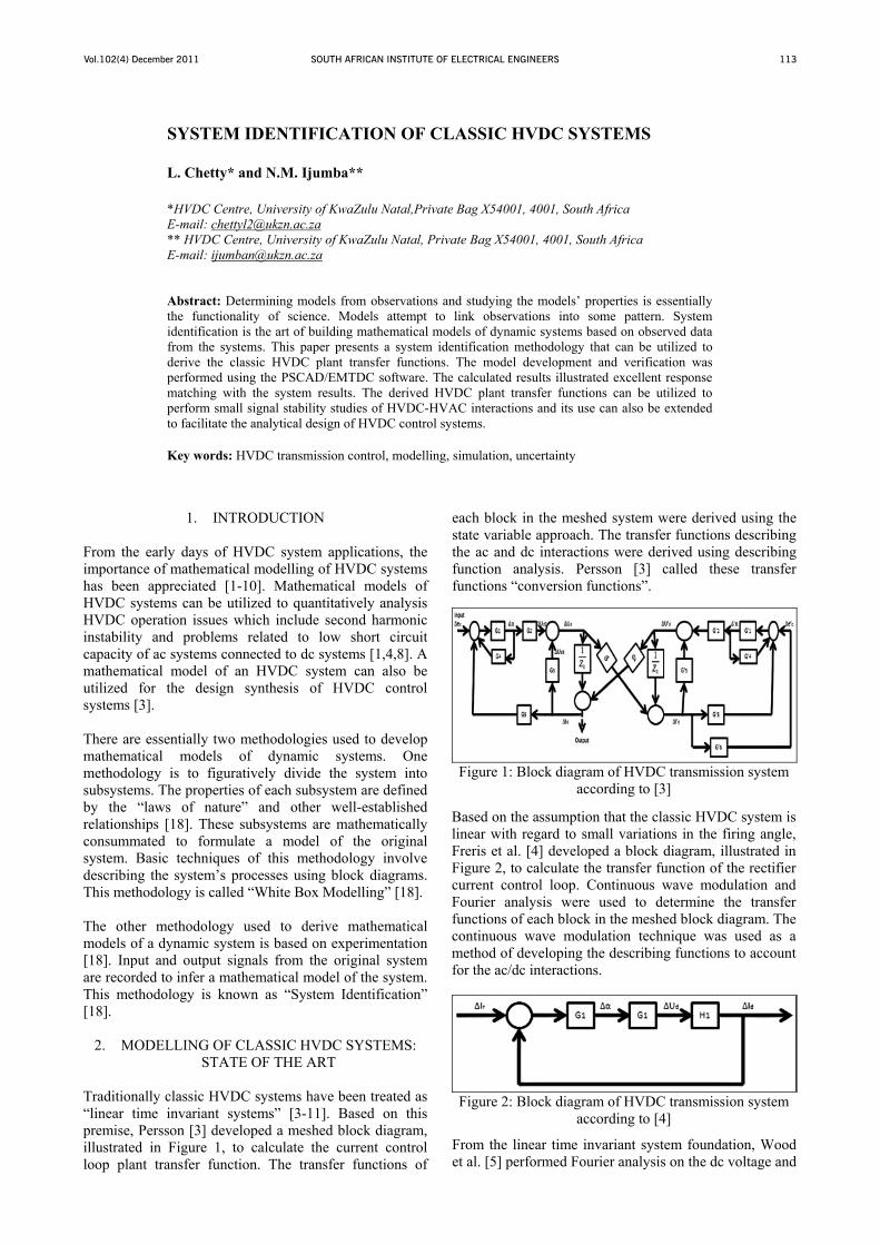
Vol.102(4) December 2011 SOUTH AFRICAN INSTITUTE OF ELECTRICAL ENGINEERS 113
SYSTEM IDENTIFICATION OF CLASSIC HVDC SYSTEMS L. Chetty* and N.M. Ijumba** *HVDC Centre, University of KwaZulu Natal,Private Bag X54001, 4001, South Africa E-mail: [email protected] ** HVDC Centre, University of KwaZulu Natal, Private Bag X54001, 4001, South Africa E-mail: [email protected] Abstract: Determining models from observations and studying the models’ properties is essentially the functionality of science. Models attempt to link observations into some pattern. System identification is the art of building mathematical models of dynamic systems based on observed data from the systems. This paper presents a system identification methodology that can be utilized to derive the classic HVDC plant transfer functions. The model development and verification was performed using the PSCAD/EMTDC software. The calculated results illustrated excellent response matching with the system results. The derived HVDC plant transfer functions can be utilized to perform small signal stability studies of HVDC-HVAC interactions and its use can also be extended to facilitate the analytical design of HVDC control systems. Key words: HVDC transmission control, modelling, simulation, uncertainty
1. INTRODUCTION
From the early days of HVDC system applications, the importance of mathematical modelling of HVDC systems has been appreciated [1-10]. Mathematical models of HVDC systems can be utilized to quantitatively analysis HVDC operation issues which include second harmonic instability and problems related to low short circuit capacity of ac systems connected to dc systems [1,4,8]. A mathematical model of an HVDC system can also be utilized for the design synthesis of HVDC control systems [3]. There are essentially two methodologies used to develop mathematical models of dynamic systems. One methodology is to figuratively divide the system into subsystems. The properties of each subsystem are defined by the “laws of nature” and other well-established relationships [18]. These subsystems are mathematically consummated to formulate a model of the original system. Basic techniques of this methodology involve describing the system’s processes using block diagrams. This methodology is called “White Box Modelling” [18]. The other methodology used to derive mathematical models of a dynamic system is based on experimentation [18]. Input and output signals from the original system are recorded to infer a mathematical model of the system. This methodology is known as “System Identification” [18].
2. MODELLING OF CLASSIC HVDC SYSTEMS: STATE OF THE ART
Traditionally classic HVDC systems have been treated as “linear time invariant systems” [3-11]. Based on this premise, Persson [3] developed a meshed block diagram, illustrated in Figure 1, to calculate the current control loop plant transfer function. The transfer functions of
each block in the meshed system were derived using the state variable approach. The transfer functions describing the ac and dc interactions were derived using describing function analysis. Persson [3] called these transfer functions “conversion functions”.
Figure 1: Block diagram of HVDC transmission system
according to [3] Based on the assumption that the classic HVDC system is linear with regard to small variations in the firing angle, Freris et al. [4] developed a block diagram, illustrated in Figure 2, to calculate the transfer function of the rectifier current control loop. Continuous wave modulation and Fourier analysis were used to determine the transfer functions of each block in the meshed block diagram. The continuous wave modulation technique was used as a method of developing the describing functions to account for the ac/dc interactions.
Figure 2: Block diagram of HVDC transmission system
according to [4] From the linear time invariant system foundation, Wood et al. [5] performed Fourier analysis on the dc voltage and
Figure 1: Block diagram of HVDC transmission system
according to [3]
Based on the assumption that the classic HVDC system is linear with regard to small variations in the firing angle, Freris et al. [4] developed a block diagram, illustrated in Figure 2, to calculate the transfer function of the rectifier current control loop. Continuous wave modulation and Fourier analysis were used to determine the transfer functions of each block in the meshed block diagram. The continuous wave modulation technique was used as a method of developing the describing functions to account for the ac/dc interactions.
Figure 2: Block diagram of HVDC transmission system
according to [4]
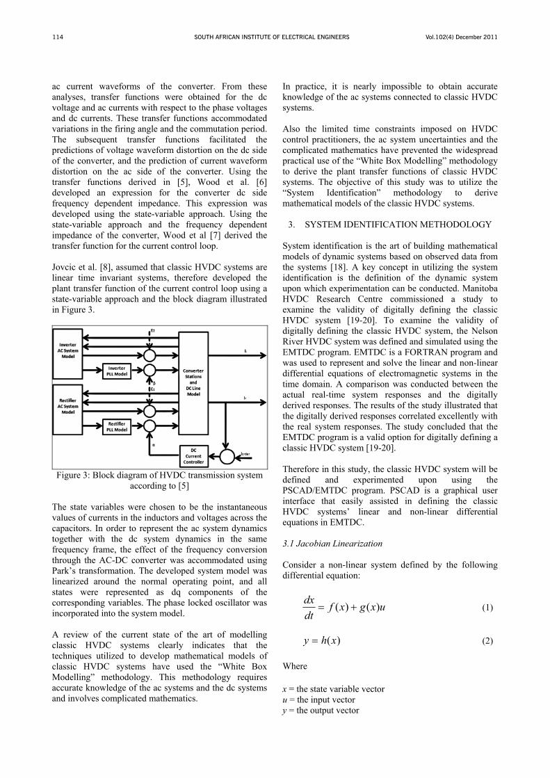
Vol.102(4) December 2011SOUTH AFRICAN INSTITUTE OF ELECTRICAL ENGINEERS114
ac current waveforms of the converter. From these analyses, transfer functions were obtained for the dc voltage and ac currents with respect to the phase voltages and dc currents. These transfer functions accommodated variations in the firing angle and the commutation period. The subsequent transfer functions facilitated the predictions of voltage waveform distortion on the dc side of the converter, and the prediction of current waveform distortion on the ac side of the converter. Using the transfer functions derived in [5], Wood et al. [6] developed an expression for the converter dc side frequency dependent impedance. This expression was developed using the state-variable approach. Using the state-variable approach and the frequency dependent impedance of the converter, Wood et al [7] derived the transfer function for the current control loop. Jovcic et al. [8], assumed that classic HVDC systems are linear time invariant systems, therefore developed the plant transfer function of the current control loop using a state-variable approach and the block diagram illustrated in Figure 3.
Figure 3: Block diagram of HVDC transmission system
according to [5] The state variables were chosen to be the instantaneous values of currents in the inductors and voltages across the capacitors. In order to represent the ac system dynamics together with the dc system dynamics in the same frequency frame, the effect of the frequency conversion through the AC-DC converter was accommodated using Park’s transformation. The developed system model was linearized around the normal operating point, and all states were represented as dq components of the corresponding variables. The phase locked oscillator was incorporated into the system model. A review of the current state of the art of modelling classic HVDC systems clearly indicates that the techniques utilized to develop mathematical models of classic HVDC systems have used the “White Box Modelling” methodology. This methodology requires accurate knowledge of the ac systems and the dc systems and involves complicated mathematics.
In practice, it is nearly impossible to obtain accurate knowledge of the ac systems connected to classic HVDC systems. Also the limited time constraints imposed on HVDC control practitioners, the ac system uncertainties and the complicated mathematics have prevented the widespread practical use of the “White Box Modelling” methodology to derive the plant transfer functions of classic HVDC systems. The objective of this study was to utilize the “System Identification” methodology to derive mathematical models of the classic HVDC systems.
3. SYSTEM IDENTIFICATION METHODOLOGY
System identification is the art of building mathematical models of dynamic systems based on observed data from the systems [18]. A key concept in utilizing the system identification is the definition of the dynamic system upon which experimentation can be conducted. Manitoba HVDC Research Centre commissioned a study to examine the validity of digitally defining the classic HVDC system [19-20]. To examine the validity of digitally defining the classic HVDC system, the Nelson River HVDC system was defined and simulated using the EMTDC program. EMTDC is a FORTRAN program and was used to represent and solve the linear and non-linear differential equations of electromagnetic systems in the time domain. A comparison was conducted between the actual real-time system responses and the digitally derived responses. The results of the study illustrated that the digitally derived responses correlated excellently with the real system responses. The study concluded that the EMTDC program is a valid option for digitally defining a classic HVDC system [19-20]. Therefore in this study, the classic HVDC system will be defined and experimented upon using the PSCAD/EMTDC program. PSCAD is a graphical user interface that easily assisted in defining the classic HVDC systems’ linear and non-linear differential equations in EMTDC. 3.1 Jacobian Linearization Consider a non-linear system defined by the following differential equation:
uxgxfdtdx )()( (1)
)(xhy (2)
Where x = the state variable vector u = the input vector y = the output vector
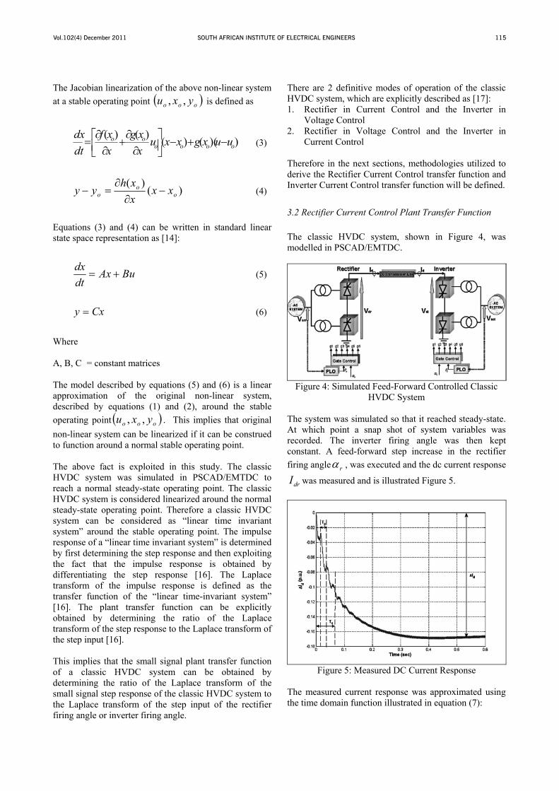
Vol.102(4) December 2011 SOUTH AFRICAN INSTITUTE OF ELECTRICAL ENGINEERS 115
The Jacobian linearization of the above non-linear system at a stable operating point ooo yxu ,, is defined as
))(()()()(oooo
oo uuxgxxuxxg
xxf
dtdx
(3)
)()(
oo
o xxxxh
yy (4)
Equations (3) and (4) can be written in standard linear state space representation as [14]:
BuAxdtdx
(5)
Cxy (6)
Where A, B, C = constant matrices The model described by equations (5) and (6) is a linear approximation of the original non-linear system, described by equations (1) and (2), around the stable operating point ooo yxu ,, . This implies that original non-linear system can be linearized if it can be construed to function around a normal stable operating point. The above fact is exploited in this study. The classic HVDC system was simulated in PSCAD/EMTDC to reach a normal steady-state operating point. The classic HVDC system is considered linearized around the normal steady-state operating point. Therefore a classic HVDC system can be considered as “linear time invariant system” around the stable operating point. The impulse response of a “linear time invariant system” is determined by first determining the step response and then exploiting the fact that the impulse response is obtained by differentiating the step response [16]. The Laplace transform of the impulse response is defined as the transfer function of the “linear time-invariant system” [16]. The plant transfer function can be explicitly obtained by determining the ratio of the Laplace transform of the step response to the Laplace transform of the step input [16]. This implies that the small signal plant transfer function of a classic HVDC system can be obtained by determining the ratio of the Laplace transform of the small signal step response of the classic HVDC system to the Laplace transform of the step input of the rectifier firing angle or inverter firing angle.
There are 2 definitive modes of operation of the classic HVDC system, which are explicitly described as [17]: 1. Rectifier in Current Control and the Inverter in
Voltage Control 2. Rectifier in Voltage Control and the Inverter in
Current Control
Therefore in the next sections, methodologies utilized to derive the Rectifier Current Control transfer function and Inverter Current Control transfer function will be defined.
3.2 Rectifier Current Control Plant Transfer Function The classic HVDC system, shown in Figure 4, was modelled in PSCAD/EMTDC.
Figure 4: Simulated Feed-Forward Controlled Classic
HVDC System The system was simulated so that it reached steady-state. At which point a snap shot of system variables was recorded. The inverter firing angle was then kept constant. A feed-forward step increase in the rectifier firing angle r , was executed and the dc current response
drI was measured and is illustrated Figure 5.
Figure 5: Measured DC Current Response
The measured current response was approximated using the time domain function illustrated in equation (7):
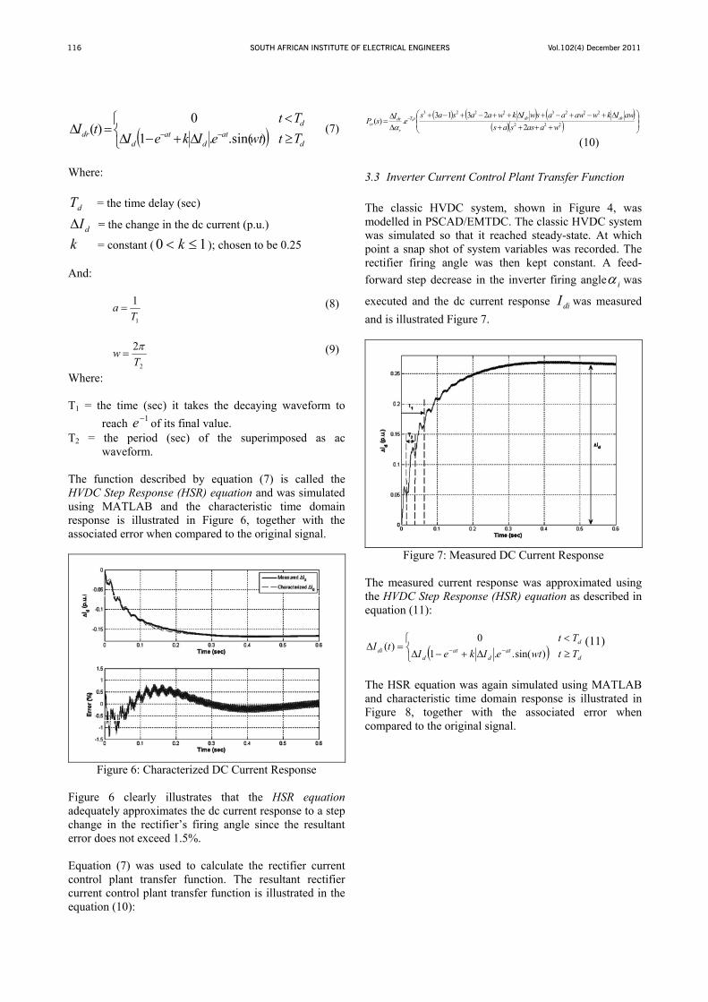
Vol.102(4) December 2011SOUTH AFRICAN INSTITUTE OF ELECTRICAL ENGINEERS116
dat
dat
d
ddr TtwteIkeI
TttI
)sin(..10
)( (7)
Where:
dT = the time delay (sec)
dI = the change in the dc current (p.u.)
k = constant ( 10 k ); chosen to be 0.25 And:
1
1T
a (8)
2
2T
w (9)
Where: T1 = the time (sec) it takes the decaying waveform to
reach 1e of its final value. T2 = the period (sec) of the superimposed as ac
waveform. The function described by equation (7) is called the HVDC Step Response (HSR) equation and was simulated using MATLAB and the characteristic time domain response is illustrated in Figure 6, together with the associated error when compared to the original signal.
Figure 6: Characterized DC Current Response
Figure 6 clearly illustrates that the HSR equation adequately approximates the dc current response to a step change in the rectifier’s firing angle since the resultant error does not exceed 1.5%. Equation (7) was used to calculate the rectifier current control plant transfer function. The resultant rectifier current control plant transfer function is illustrated in the equation (10):
222
22232223
22313
.)(waassas
awIkwawaaswIkwaasaseIsP drdrsT
r
drcr
d
(10)
3.3 Inverter Current Control Plant Transfer Function The classic HVDC system, shown in Figure 4, was modelled in PSCAD/EMTDC. The classic HVDC system was simulated so that it reached steady-state. At which point a snap shot of system variables was recorded. The rectifier firing angle was then kept constant. A feed-forward step decrease in the inverter firing angle i was
executed and the dc current response diI was measured and is illustrated Figure 7.
Figure 7: Measured DC Current Response
The measured current response was approximated using the HVDC Step Response (HSR) equation as described in equation (11):
dat
dat
d
ddi TtwteIkeI
TttI
)sin(..10
)( (11)
The HSR equation was again simulated using MATLAB and characteristic time domain response is illustrated in Figure 8, together with the associated error when compared to the original signal.
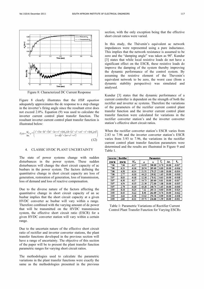
Vol.102(4) December 2011 SOUTH AFRICAN INSTITUTE OF ELECTRICAL ENGINEERS 117
Figure 8: Characterized DC Current Response
Figure 8 clearly illustrates that the HSR equation adequately approximates the dc response to a step change in the inverter’s firing angle since the resultant error does not exceed 2.0%. Equation (9) was used to calculate the inverter current control plant transfer function. The resultant inverter current control plant transfer function is illustrated below:
222
22232223
22313
.)(waassas
awIkwawaaswIkwaasaseIsP didisT
i
dici
d
(12)
4. CLASSIC HVDC PLANT UNCERTAINTY
The state of power systems change with sudden disturbances in the power system. These sudden disturbances will change the short circuit capacity of ac busbars in the power system. The factors defining the quantitative change in short circuit capacity are loss of generation, restoration of generation, loss of transmission, loss of demand and loss of reactive compensation. Due to the diverse nature of the factors affecting the quantitative change in short circuit capacity of an ac busbar implies that the short circuit capacity at a given HVDC converter ac busbar will vary within a range. Therefore combined with the varying amount of dc power that will be transmitted on the HVDC transmission system, the effective short circuit ratio (ESCR) for a given HVDC converter station will vary within a certain range. Due to the uncertain nature of the effective short circuit ratio of rectifier and inverter converter stations, the plant transfer functions developed in the previous section will have a range of uncertainty. The objective of this section of the paper will be to present the plant transfer function parametric ranges for varying short circuit ratios. The methodologies used to calculate the parametric variations in the plant transfer functions were exactly the same as the methodologies presented in the previous
section, with the only exception being that the effective short circuit ratios were varied. In this study, the Thévenin’s equivalent ac network impedances were represented using a pure inductance. This implies that the network resistance is assumed to be zero and the “damping angle” was taken as 90o. Kundur [3] states that while local resistive loads do not have a significant effect on the ESCR, these resistive loads do improve the damping of the system thereby improving the dynamic performance of the control system. By assuming the resistive element of the Thevenin’s equivalent network to be zero, the worst case (from a dynamic stability perspective) was simulated and analysed. Kundur [3] states that the dynamic performance of a current controller is dependent on the strength of both the rectifier and inverter ac systems. Therefore the variations of the parameters of the rectifier current control plant transfer function and the inverter current control plant transfer function were calculated for variations in the rectifier converter station’s and the inverter converter station’s effective short circuit ratios. When the rectifier converter station’s ESCR varies from 2.83 to 7.96 and the inverter converter station’s ESCR varies from 3.93 to 7.96, the variations in the rectifier current control plant transfer function parameters were determined and the results are illustrated in Figure 9 and Table 1.
Table 1: Parametric Variations of Rectifier Current Control Plant Transfer Function for Varying ESCRs
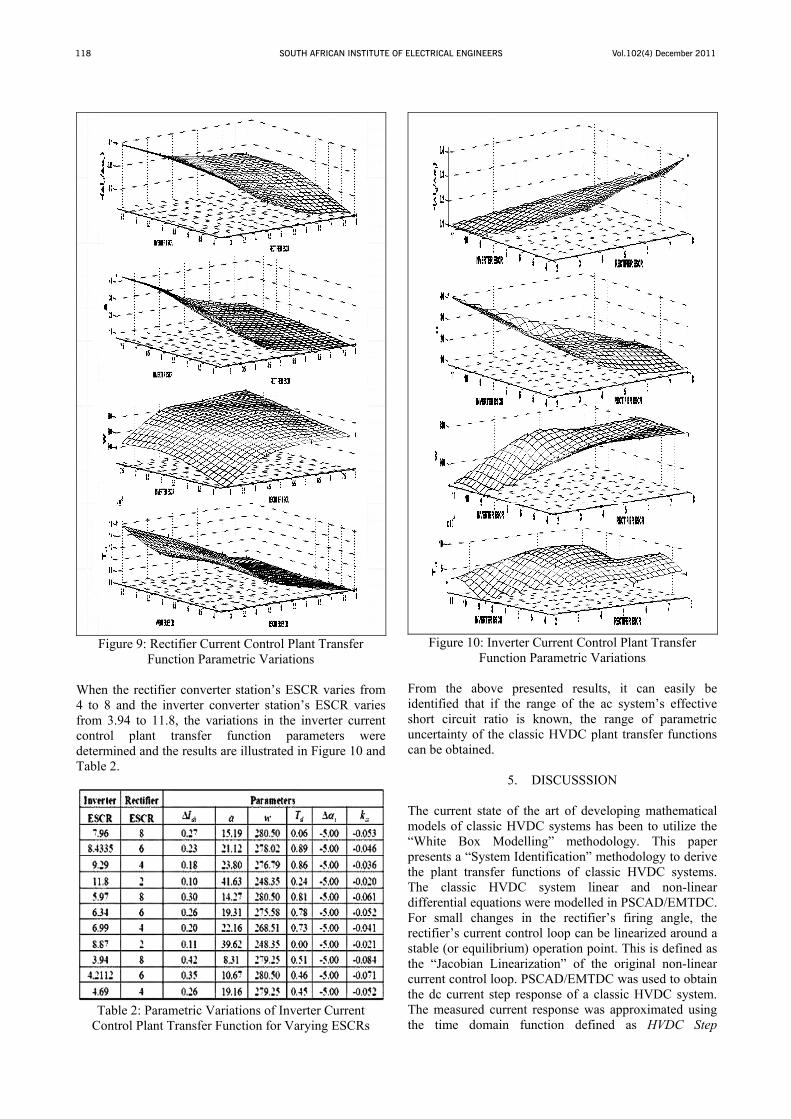
Vol.102(4) December 2011SOUTH AFRICAN INSTITUTE OF ELECTRICAL ENGINEERS118
Figure 9: Rectifier Current Control Plant Transfer
Function Parametric Variations When the rectifier converter station’s ESCR varies from 4 to 8 and the inverter converter station’s ESCR varies from 3.94 to 11.8, the variations in the inverter current control plant transfer function parameters were determined and the results are illustrated in Figure 10 and Table 2.
Table 2: Parametric Variations of Inverter Current
Control Plant Transfer Function for Varying ESCRs
Figure 10: Inverter Current Control Plant Transfer
Function Parametric Variations
From the above presented results, it can easily be identified that if the range of the ac system’s effective short circuit ratio is known, the range of parametric uncertainty of the classic HVDC plant transfer functions can be obtained.
5. DISCUSSSION
The current state of the art of developing mathematical models of classic HVDC systems has been to utilize the “White Box Modelling” methodology. This paper presents a “System Identification” methodology to derive the plant transfer functions of classic HVDC systems. The classic HVDC system linear and non-linear differential equations were modelled in PSCAD/EMTDC. For small changes in the rectifier’s firing angle, the rectifier’s current control loop can be linearized around a stable (or equilibrium) operation point. This is defined as the “Jacobian Linearization” of the original non-linear current control loop. PSCAD/EMTDC was used to obtain the dc current step response of a classic HVDC system. The measured current response was approximated using the time domain function defined as HVDC Step
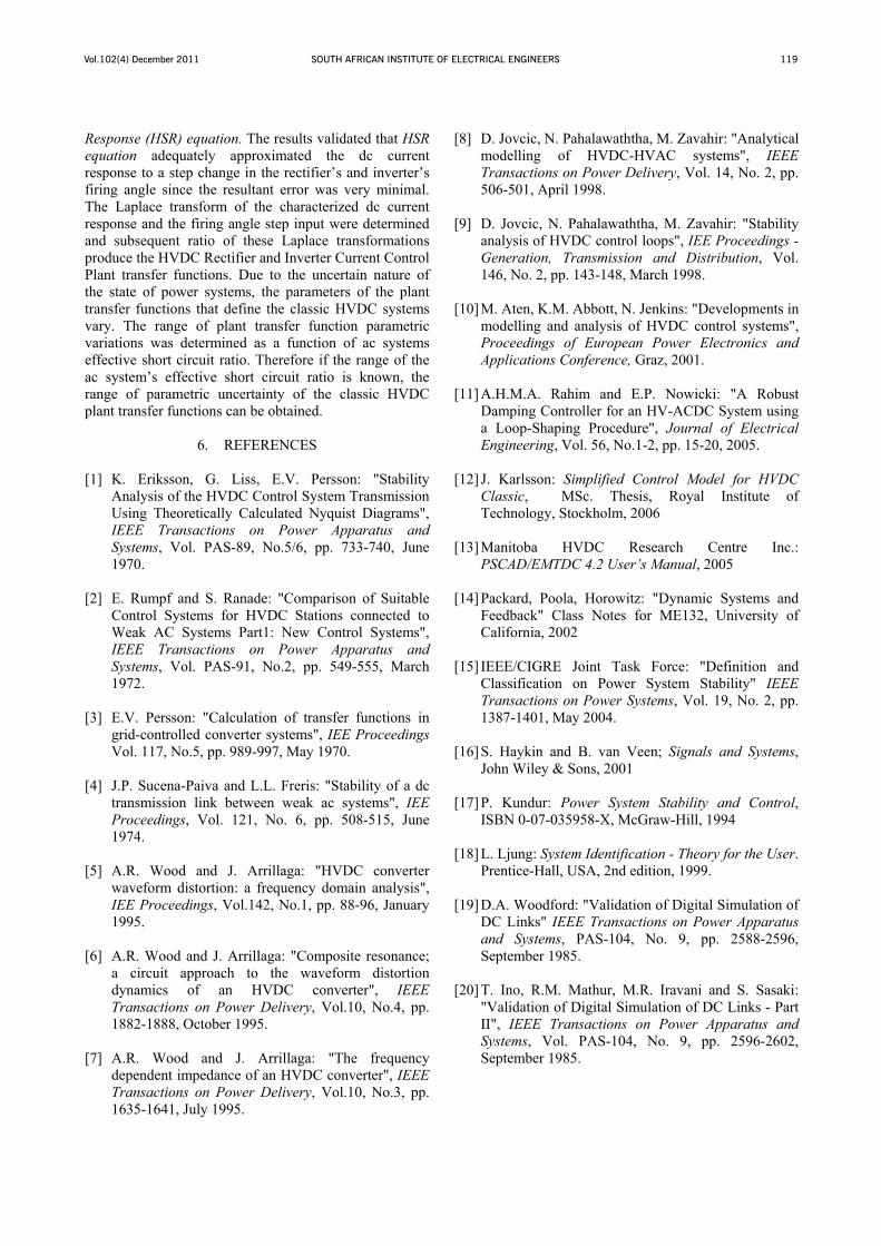
Vol.102(4) December 2011 SOUTH AFRICAN INSTITUTE OF ELECTRICAL ENGINEERS 119
Response (HSR) equation. The results validated that HSR equation adequately approximated the dc current response to a step change in the rectifier’s and inverter’s firing angle since the resultant error was very minimal. The Laplace transform of the characterized dc current response and the firing angle step input were determined and subsequent ratio of these Laplace transformations produce the HVDC Rectifier and Inverter Current Control Plant transfer functions. Due to the uncertain nature of the state of power systems, the parameters of the plant transfer functions that define the classic HVDC systems vary. The range of plant transfer function parametric variations was determined as a function of ac systems effective short circuit ratio. Therefore if the range of the ac system’s effective short circuit ratio is known, the range of parametric uncertainty of the classic HVDC plant transfer functions can be obtained.
6. REFERENCES
[1] K. Eriksson, G. Liss, E.V. Persson: "Stability Analysis of the HVDC Control System Transmission Using Theoretically Calculated Nyquist Diagrams", IEEE Transactions on Power Apparatus and Systems, Vol. PAS-89, No.5/6, pp. 733-740, June 1970.
[2] E. Rumpf and S. Ranade: "Comparison of Suitable Control Systems for HVDC Stations connected to Weak AC Systems Part1: New Control Systems", IEEE Transactions on Power Apparatus and Systems, Vol. PAS-91, No.2, pp. 549-555, March 1972.
[3] E.V. Persson: "Calculation of transfer functions in
grid-controlled converter systems", IEE Proceedings Vol. 117, No.5, pp. 989-997, May 1970.
[4] J.P. Sucena-Paiva and L.L. Freris: "Stability of a dc
transmission link between weak ac systems", IEE Proceedings, Vol. 121, No. 6, pp. 508-515, June 1974.
[5] A.R. Wood and J. Arrillaga: "HVDC converter waveform distortion: a frequency domain analysis", IEE Proceedings, Vol.142, No.1, pp. 88-96, January 1995.
[6] A.R. Wood and J. Arrillaga: "Composite resonance; a circuit approach to the waveform distortion dynamics of an HVDC converter", IEEE Transactions on Power Delivery, Vol.10, No.4, pp. 1882-1888, October 1995.
[7] A.R. Wood and J. Arrillaga: "The frequency dependent impedance of an HVDC converter", IEEE Transactions on Power Delivery, Vol.10, No.3, pp. 1635-1641, July 1995.
[8] D. Jovcic, N. Pahalawaththa, M. Zavahir: "Analytical modelling of HVDC-HVAC systems", IEEE Transactions on Power Delivery, Vol. 14, No. 2, pp. 506-501, April 1998.
[9] D. Jovcic, N. Pahalawaththa, M. Zavahir: "Stability analysis of HVDC control loops", IEE Proceedings - Generation, Transmission and Distribution, Vol. 146, No. 2, pp. 143-148, March 1998.
[10] M. Aten, K.M. Abbott, N. Jenkins: "Developments in modelling and analysis of HVDC control systems", Proceedings of European Power Electronics and Applications Conference, Graz, 2001.
[11] A.H.M.A. Rahim and E.P. Nowicki: "A Robust
Damping Controller for an HV-ACDC System using a Loop-Shaping Procedure", Journal of Electrical Engineering, Vol. 56, No.1-2, pp. 15-20, 2005.
[12] J. Karlsson: Simplified Control Model for HVDC Classic, MSc. Thesis, Royal Institute of Technology, Stockholm, 2006
[13] Manitoba HVDC Research Centre Inc.:
PSCAD/EMTDC 4.2 User’s Manual, 2005
[14] Packard, Poola, Horowitz: "Dynamic Systems and Feedback" Class Notes for ME132, University of California, 2002
[15] IEEE/CIGRE Joint Task Force: "Definition and Classification on Power System Stability" IEEE Transactions on Power Systems, Vol. 19, No. 2, pp. 1387-1401, May 2004.
[16] S. Haykin and B. van Veen; Signals and Systems, John Wiley & Sons, 2001
[17] P. Kundur: Power System Stability and Control, ISBN 0-07-035958-X, McGraw-Hill, 1994
[18] L. Ljung: System Identification - Theory for the User. Prentice-Hall, USA, 2nd edition, 1999.
[19] D.A. Woodford: "Validation of Digital Simulation of DC Links" IEEE Transactions on Power Apparatus and Systems, PAS-104, No. 9, pp. 2588-2596, September 1985.
[20] T. Ino, R.M. Mathur, M.R. Iravani and S. Sasaki: "Validation of Digital Simulation of DC Links - Part II", IEEE Transactions on Power Apparatus and Systems, Vol. PAS-104, No. 9, pp. 2596-2602, September 1985.

Vol.102(4) December 2011SOUTH AFRICAN INSTITUTE OF ELECTRICAL ENGINEERS120
Notes