Approximation Algorithms for Stochastic k-TSP∗

Alina Ene1, Viswanath Nagarajan2, and Rishi Saket3

1 Computer Science Department, Boston University. aene@bu.edu2 Industrial and Operations Engineering Department, University of Michigan.

viswa@umich.edu3 IBM Research India. rissaket@in.ibm.com

AbstractThis paper studies the stochastic variant of the classical k-TSP problem where rewards at thevertices are independent random variables which are instantiated upon the tour’s visit. Theobjective is to minimize the expected length of a tour that collects reward at least k. Thesolution is a policy describing the tour which may (adaptive) or may not (non-adaptive) dependon the observed rewards. Our work presents an adaptive O(log k)-approximation algorithmfor Stochastic k-TSP, along with a non-adaptive O(log2 k)-approximation algorithm whichalso upper bounds the adaptivity gap by O(log2 k). We also show that the adaptivity gap ofStochastic k-TSP is at least e, even in the special case of stochastic knapsack cover.

1998 ACM Subject Classification F.2.2 Nonnumerical Algorithms and Problems

Keywords and phrases Stochastic TSP, algorithms, approximation, adaptivity gap

Digital Object Identifier 10.4230/LIPIcs.FSTTCS.2017.27

1 Introduction

In this paper, we consider the following stochastic variant of the classical k-TSP problem.The input consists of a metric (V, d) with depot r ∈ V . Each vertex v ∈ V has an independentstochastic reward Rv ∈ Z+. All reward distributions are given as input and thus they areknown upfront, but the actual reward instantiation Rv is only known when vertex v isvisited. Given a target value k, the goal is to find an adaptive tour originating from r thatcollects a total reward at least k with the minimum expected length.1 We assume that allrewards are supported on 0, 1, . . . , k.

Any feasible solution to this problem can be described by a decision tree where nodescorrespond to vertices that are visited and branches correspond to observed reward instanti-ations. The size of such decision trees can be exponentially large. So we focus on obtainingsolutions (aka policies) that implicitly specify decision trees. These solutions are called adap-tive because the choice of the next vertex to visit depends on past random instantiations.

We will also consider the special class of non-adaptive solutions. Such a solution isdescribed simply by an ordered list of vertices: the policy involves visiting vertices in thegiven order until the target of k is met (at which point the tour returns to r). Thesesolutions are often preferred over adaptive solutions as they are easier to implement inpractice. However, the performance of non-adaptive solutions may be much worse, and so itis important to bound the adaptivity gap [15] which is the worst-case ratio between optimal

∗ This work was partly done when the authors were at the IBM T. J. Watson Research Center.1 If the total instantiated reward

∑v∈V

Rv happens to be less than k, the tour ends after visiting allvertices.

© Alina Ene, Viswanath Nagarajan, and Rishi Saket;licensed under Creative Commons License CC-BY

37th IARCS Annual Conference on Foundations of Software Technology and Theoretical Computer Science(FSTTCS 2017).Editors: Satya Lokam and R. Ramanujam; Article No. 27; pp. 27:1–27:14

Leibniz International Proceedings in InformaticsSchloss Dagstuhl – Leibniz-Zentrum für Informatik, Dagstuhl Publishing, Germany

27:2 Approximation Algorithms for Stochastic k-TSP

adaptive and non-adaptive policies. This approach via non-adaptive policies has been veryuseful for a number of stochastic optimization problems, eg. [15, 19, 22, 5, 23, 24, 6, 25].

The Stochastic k-TSP problem captures several well-studied problems, including theclassical k-TSP problem where the rewards are deterministic, and the stochastic knapsackcover problem where the metric (V, d) is a weighted star rooted at r: given n items witheach item i ∈ [n] having deterministic cost di and independent random reward Ri ∈ Z+, anda target k, find an adaptive policy that obtains total reward k at the minimum expectedcost. The k-TSP problem (and the related spanning tree variant k-MST) have receivedconsiderable attention, leading to the development of a 2-approximation algorithm for theproblem [18]. The stochastic knapsack cover problem was considered recently in [16], wherean adaptive 2-approximation algorithm was obtained; however, no bounds on the adaptivitygap were known previously even for this special case.

Results and Techniques. In this paper, we give the first approximation algorithm forthe general stochastic k-TSP, with an approximation ratio of O(log k). We also show thatthe adaptivity gap is O(log2 k). The adaptivity gap is constructive: we give a non-adaptivealgorithm that is an O(log2 k)-approximation to the optimal adaptive policy.

I Theorem 1. There is an adaptive algorithm for stochastic k-TSP with approximationratio O(log k). Moreover, the adaptivity gap is upper bounded by O(log2 k).

To motivate our approach, consider an algorithm for the classical k-TSP problem whichhas access to a hypothetical2 subroutine exactly solving the deterministic orienteering prob-lem: given a metric (V, d) on vertices with non-negative reward, a root vertex r, and a boundt compute a tour starting at r of length at most t which collects the maximum reward. Thealgorithm iterates over tour lengths of increasing powers of 2, solving for each length thedeterministic orienteering problem, until the union of the computed tours yields reward k.It can be seen that this is an O(1)-approximation to k-TSP. Our algorithm adapts this iter-ative method to Stochastic k-TSP using the expected truncated rewards at each vertex.At the beginning of each iteration, the rewards distribution at each vertex is appropriatelytruncated w.r.t. the residual target (and set to zero if the vertex has been previously visited).However, in the stochastic setting, even if we used an exact orienteering algorithm, we needto construct roughly (log k) tours for each length (see Example 2 in Section 2.1). We showthat using O(log k) many tours of each length suffices to obtain an O(log k)-approximationalgorithm for stochastic k-TSP. Moreover, this multiple-tour approach also allows for theuse of an O(1)-approximation for orienteering, which is needed for a poly-time algorithm.

The high-level idea in the analysis is to show that the non-completion probability in thealgorithm drops (roughly) by a constant factor in each iteration. This approach is similarto that for the classic min-latency TSP [10, 17]. Such an approach has also been used forstochastic optimization problems in [27, 28], but those results do not apply directly to metric-based costs that we need to handle here. Our main technical contribution is in proving thebound on non-completion probabilities in successive iterations (Lemma 3). This involvesupper and lower bounding the expected “relative gain” which is the expected (truncated)increase in reward divided by the residual target. See Section 2 for details.

The non-adaptive algorithm is based on “simulating” the above adaptive algorithm.Corresponding to each orienteering instance solved in the adaptive algorithm we now solvelog2 k different instances based on different power-of-two values for the residual target. This

2 We do not expect a poly-time exact algorithm for orienteering as the problem is APX-hard [9].

A. Ene, V. Nagarajan, and R. Saket 27:3

results in a worse O(log2 k) approximation ratio; this is relative to the optimal adaptivevalue and hence it bounds the adaptivity gap. We are not aware of a more direct approachfor the non-adaptive problem, even if we compare to the optimal non-adaptive value.

We also show that the adaptivity gap is at least e ≈ 2.718, which holds even in thespecial case of stochastic knapsack cover with a single random item.

I Theorem 2. The adaptivity gap of Stochastic k-TSP (knapsack cover) is at least e.

This result is obtained in an indirect manner. Using LP-duality we show that random-ized online lower bounds for the online bidding problem [13] can be reduced to adaptivitygap lower bounds for stochastic knapsack-cover. These lower bound instances contain asingle stochastic item. We can also show using a connection to the incremental k-MSTproblem [29], that the adaptivity gap for such instances is exactly e.

Other related work. Stochastic packing and covering problems have received considerableattention, leading to approximation guarantees and adaptivity gaps for several importantproblems, including knapsack [15, 8, 30, 16], packing and covering integer programs [14, 19],matching [12, 5, 1, 7, 2], matroid intersection [25, 3], submodular cover [20, 27, 21, 28], andorienteering [22, 24, 6]. Recently, [26] proved a constant adaptivity gap for submodular max-imization problems under a very general class of constraints (including orienteering). Thisis however not directly applicable to stochastic k-TSP because we have (i) a minimizationobjective with strict covering requirement and (ii) general random variables as opposed tojust binary in [26].

Sections 2 and 3 describe and analyze the adaptive and non-adaptive algorithms respec-tively for Stochastic k-TSP. Together they prove Theorem 1. The lower bound on theadaptivity gap (Theorem 2) is proved in Section 4.

2 Stochastic k-TSP Algorithm

Let us begin with an informal description of the adaptive algorithm. The algorithm relies oniteratively solving instances of the (deterministic) orienteering problem. In the orienteeringproblem, we are given a metric (V, d), depot r, profits at vertices and a length boundB; the goal is to find a tour originating from r of length at most B that maximizes thetotal profit. There is a (2 + ε)-approximation algorithm for orienteering [11] which wecan use directly. The vertex-profits in the orienteering instance are chosen to be truncatedexpectations of the random rewards Rv where the truncation threshold is the current residualtarget. The length bounds are geometrically increasing with the phases of the algorithm.The algorithm terminates when the residual target reaches zero or all the vertices havebeen visited. However, in each phase the algorithm solves α ≈ (log k) many iterationseach approximately solving the residual orienteering instance with the same length boundof that phase. This (roughly speaking) results in the O(log k) approximation ratio. Therequirement of many iterations per phase turns out to be a somewhat subtle issue: we showin Section 2.1 that significantly reducing the number of repetitions results in a much worseapproximation ratio.

The formal algorithm is given below. We assume (by scaling) that the minimum positivedistance in the metric (V, d) is one. At any point in the algorithm, S denotes the set ofcurrently visited vertices, σ denotes the reward instantiations of S, and k(σ) is the totalobserved reward. The number of iterations of the inner for-loop is α := c ·Hk, where c ≥ 1is a constant to be fixed later and Hk ≈ ln k is the kth harmonic number. We will showthat Ad-kTSP is an 8α-approximation algorithm for Stochastic k-TSP.

FSTTCS 2017

27:4 Approximation Algorithms for Stochastic k-TSP

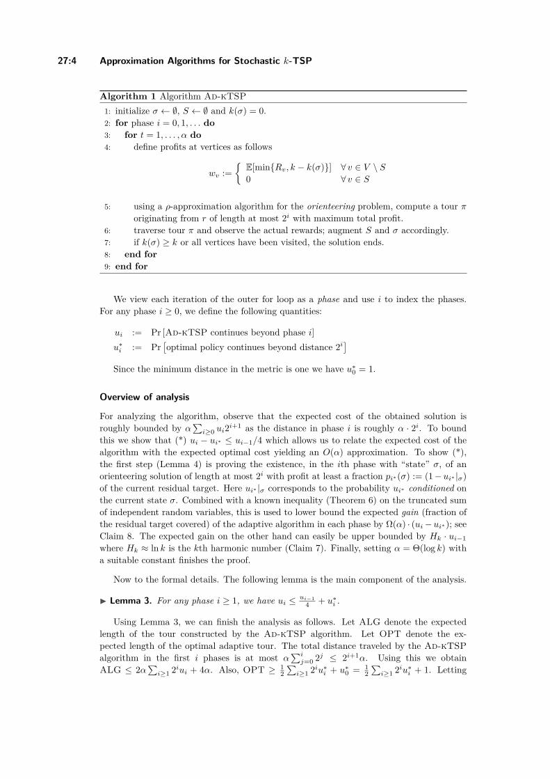
Algorithm 1 Algorithm Ad-kTSP1: initialize σ ← ∅, S ← ∅ and k(σ) = 0.2: for phase i = 0, 1, . . . do3: for t = 1, . . . , α do4: define profits at vertices as follows

wv :=

E[minRv, k − k(σ)] ∀ v ∈ V \ S0 ∀ v ∈ S

5: using a ρ-approximation algorithm for the orienteering problem, compute a tour πoriginating from r of length at most 2i with maximum total profit.

6: traverse tour π and observe the actual rewards; augment S and σ accordingly.7: if k(σ) ≥ k or all vertices have been visited, the solution ends.8: end for9: end for

We view each iteration of the outer for loop as a phase and use i to index the phases.For any phase i ≥ 0, we define the following quantities:

ui := Pr [Ad-kTSP continues beyond phase i]u∗i := Pr

[optimal policy continues beyond distance 2i

]Since the minimum distance in the metric is one we have u∗0 = 1.

Overview of analysis

For analyzing the algorithm, observe that the expected cost of the obtained solution isroughly bounded by α

∑i≥0 ui2i+1 as the distance in phase i is roughly α · 2i. To bound

this we show that (*) ui − ui∗ ≤ ui−1/4 which allows us to relate the expected cost of thealgorithm with the expected optimal cost yielding an O(α) approximation. To show (*),the first step (Lemma 4) is proving the existence, in the ith phase with “state” σ, of anorienteering solution of length at most 2i with profit at least a fraction pi∗(σ) := (1−ui∗ |σ)of the current residual target. Here ui∗ |σ corresponds to the probability ui∗ conditioned onthe current state σ. Combined with a known inequality (Theorem 6) on the truncated sumof independent random variables, this is used to lower bound the expected gain (fraction ofthe residual target covered) of the adaptive algorithm in each phase by Ω(α) · (ui−ui∗); seeClaim 8. The expected gain on the other hand can easily be upper bounded by Hk · ui−1where Hk ≈ ln k is the kth harmonic number (Claim 7). Finally, setting α = Θ(log k) witha suitable constant finishes the proof.

Now to the formal details. The following lemma is the main component of the analysis.

I Lemma 3. For any phase i ≥ 1, we have ui ≤ ui−14 + u∗i .

Using Lemma 3, we can finish the analysis as follows. Let ALG denote the expectedlength of the tour constructed by the Ad-kTSP algorithm. Let OPT denote the ex-pected length of the optimal adaptive tour. The total distance traveled by the Ad-kTSPalgorithm in the first i phases is at most α

∑ij=0 2j ≤ 2i+1α. Using this we obtain

ALG ≤ 2α∑i≥1 2iui + 4α. Also, OPT ≥ 1

2∑i≥1 2iu∗i + u∗0 = 1

2∑i≥1 2iu∗i + 1. Letting

A. Ene, V. Nagarajan, and R. Saket 27:5

T :=∑i≥1 2iui and using Lemma 3, we obtain

T ≤ 14∑i≥1

2i · ui−1 +∑i≥1

2i · u∗i ≤12∑i≥1

2i · ui +∑i≥1

2i · u∗i + 12 ≤

12T + 2 ·OPT− 3

2 .

It follows that T ≤ 4 ·OPT−3 and ALG ≤ 8α ·OPT. Thus we obtain an 8α-approximationalgorithm, which proves the first part of Theorem 1.

Now we turn to the proof of Lemma 3. We start by introducing some notation. Consideran arbitrary point in the execution of algorithm Ad-kTSP, and let 〈S, σ, k(σ)〉 be a triplein which S is the set of vertices visited so far, σ is the observed instantiation of S, and k(σ)is the total reward observed in S. We refer to such a triple 〈S, σ, k(σ)〉 as the state of thealgorithm.

I Lemma 4. Consider a state 〈S, σ, k(σ)〉 of the Ad-kTSP algorithm. Consider the Ori-enteering instance in which each vertex in S is assigned a profit of zero and each vertexv not in S is assigned a profit of E [min Rv, k − k(σ)]. There is an orienteering tour fromr of length at most 2i with profit at least (k − k(σ)) · p∗i (σ), where

p∗i (σ) = Pr[optimal policy completes before distance 2i | σ

].

Proof. Consider the tree T ∗ representing the optimal policy. We condition on the instan-tiations σ on vertices S to obtain tree T ∗(S, σ). Formally, we start with T ∗(S, σ) = T ∗and apply the following transformation for each vertex v ∈ S with instantiation σv: at eachnode ν in T ∗(S, σ) corresponding to v, we remove all subtrees of ν except the subtree cor-responding to instantiation σv; additionally, the probability of this edge (labeled σv) is setto one. Note that the probabilities at nodes corresponding to vertices V \ S are unchanged,since rewards at different vertices are independent.

Now, mark those nodes in T ∗(S, σ) that correspond to completion (i.e. reward at leastk is collected) within distance 2i. Note that the probability of reaching a marked node isexactly p∗i (σ). Finally, let T denote the subtree of T ∗(S, σ) containing only those nodesthat have a marked descendant. When tree T is traversed, the probability of reaching aleaf-node is p∗i (σ); with the remaining probability the traversal ends at some internal node.Clearly, every leaf-node in T is marked and hence corresponds to an r-tour of length at most2i along with instantiated rewards that sum to at least k. Define modified rewards at nodesof T as follows:

Rv =

minRv, k − k(σ) if v 6∈ S0 if v ∈ S

Notice that the profits in the deterministic Orienteering instance are precisely wv =E[Rv]. Observe that the sum of modified rewards at each leaf of T is at least k−k(σ). Thusthe expected R-reward obtained in T is E ≥ (k − k(σ)) · p∗i (σ). Also,

E =∑ν∈T

Pr[reach ν]·E[Rν | reach ν

]=∑ν∈T

Pr[reach ν]·E[Rν

]=∑ν∈T

Pr[end at ν]·

∑µν

wµ

.

Above, for a node ν ∈ T , we use Rν and wν to denote the respective variables for the vertex(in V ) corresponding to ν. Also, the notation µ ν refers to node µ being an ancestorof node ν in T . The first equality is by definition of E, the second uses the fact thatRv : v ∈ V are independent, and the last is an interchange of summation. By averaging,there is some node ν′ ∈ T with

∑µ≺ν′ wµ ≥ E ≥ (k− k(σ)) · p∗i (σ). We can assume that ν′

FSTTCS 2017

27:6 Approximation Algorithms for Stochastic k-TSP

is a leaf node (otherwise we can reset ν′ to be any leaf node of T below ν′). So the r-tourcorresponding to this node ν′ has length at most 2i and is feasible for the deterministicOrienteering instance. Moreover, it has profit at least (k − k(σ)) · p∗i (σ) as claimed. J

I Lemma 5. Consider a state 〈S, σ, k(σ)〉 of the Ad-kTSP algorithm with k(σ) < k.Consider the Orienteering instance with profits wv : v ∈ V where wv = 0 for v ∈ Sand wv = E [min Rv, k − k(σ)] for v 6∈ S. Let π be any ρ-approximate orienteering tourconsisting of vertices V (π). Then,

E

min

∑v∈V (π)\S

Rv, k − k(σ)

≥ 1

ρ·(

1− 1e

)· (k − k(σ))· p∗i (σ).

Proof. For each v ∈ V (π)\S define Xv := min

Rv

k−k(σ) , 1. Note that Xvs are independent

[0, 1] random variables, and E[Xv] = wv

k−k(σ) . Let X :=∑v∈V (π)\S Xv and Y = min(X, 1).

So the profit obtained by solution π to the deterministic orienteering instance is (k− k(σ)) ·E[X]. Using Lemma 4 and the fact that π is a ρ-approximate solution, we obtain E[X] ≥1ρ · p∗i . We can now complete the proof of the lemma by applying Theorem 6 below. J

I Theorem 6 ([4]). Given a set Xv of independent [0, 1] random variables with X =∑Xv

and Y = min(X, 1), we have E[Y ] ≥ (1− 1/e) ·minE[X], 1.

Now we are ready to prove Lemma 3.

Proof of Lemma 3. Consider any phase i ≥ 1 and let 〈S, σ, k(σ)〉 be the state of the Ad-kTSP algorithm at the start of some iteration of the inner loop. Let π be the orienteeringtour that the algorithm visits next. Define

gain(〈S, σ〉) :=E[min

∑v∈V (π)\S Rv, k − k(σ)

]k − k(σ) if k(σ) < k,

and gain(〈S, σ〉) := 0 if k(σ) ≥ k. The quantity gain(〈S, σ〉) measures the expected fractionof the residual target that we cover after visiting π.

Let I(σ) = [k(σ) ≥ k] be an indicator variable that is equal to one if k(σ) ≥ k and it isequal to zero otherwise. We have:

gain(〈S, σ〉) ≥ 1ρ·(

1− 1e

)· (p∗i (σ)− I(σ)) . (1)

To see this, note that if I(σ) is one, the gain is zero and the inequality above holds sincep∗i (σ) ≤ 1; and if I(σ) is zero, this inequality follows from Lemma 5.

Recall that there are α iterations of the inner loop in phase i, and we use t ∈ [α] to indexthe iterations. For each iteration t (of phase i), let St be the random variable denoting thevertices visited until iteration t, and let σt denote the reward instantiations of St. Define:

Gt := E〈St,σt〉

[gain(〈St, σt〉)]

Let ∆ =∑αt=1Gt denote the total gain in phase i. The proof relies on upper and lower

bounding ∆, which is done in the next two claims.

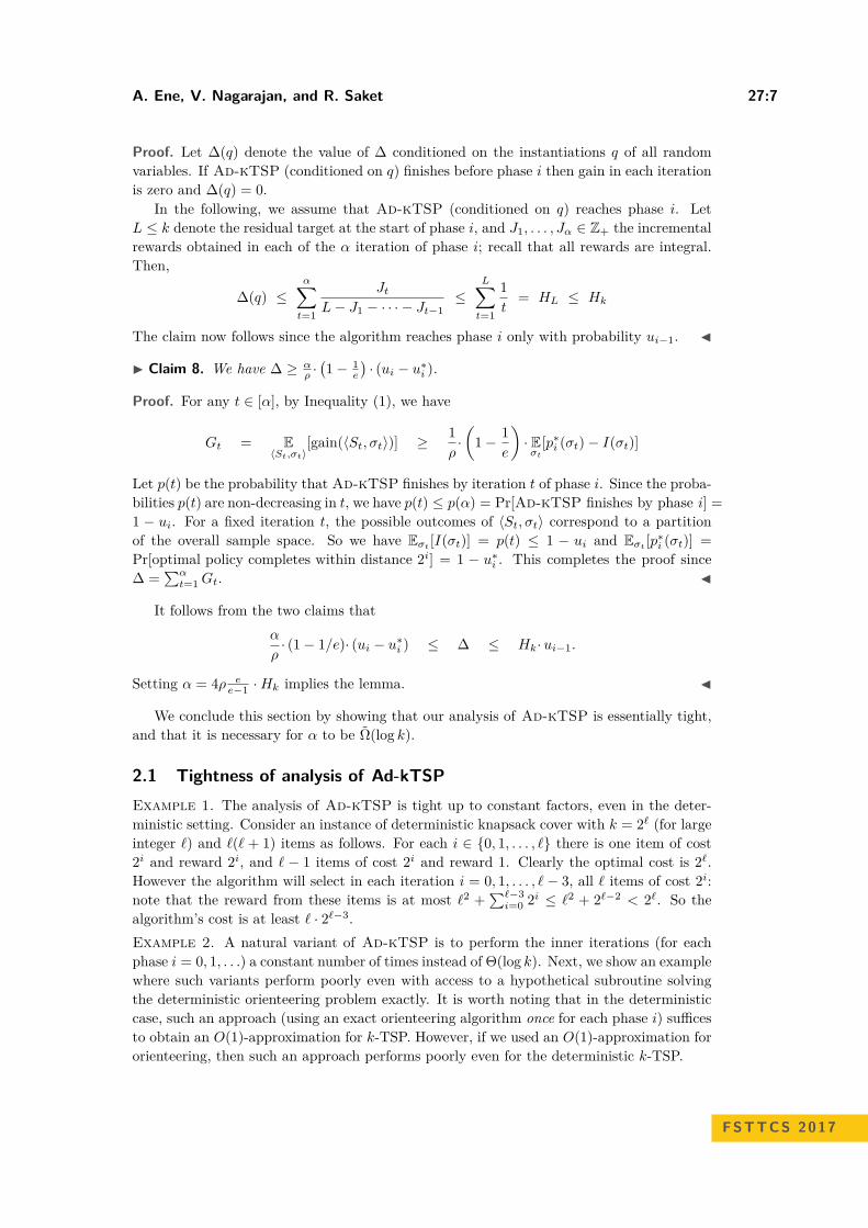
I Claim 7. We have ∆ ≤ Hk·ui−1.

A. Ene, V. Nagarajan, and R. Saket 27:7

Proof. Let ∆(q) denote the value of ∆ conditioned on the instantiations q of all randomvariables. If Ad-kTSP (conditioned on q) finishes before phase i then gain in each iterationis zero and ∆(q) = 0.

In the following, we assume that Ad-kTSP (conditioned on q) reaches phase i. LetL ≤ k denote the residual target at the start of phase i, and J1, . . . , Jα ∈ Z+ the incrementalrewards obtained in each of the α iteration of phase i; recall that all rewards are integral.Then,

∆(q) ≤α∑t=1

JtL− J1 − · · · − Jt−1

≤L∑t=1

1t

= HL ≤ Hk

The claim now follows since the algorithm reaches phase i only with probability ui−1. J

I Claim 8. We have ∆ ≥ αρ ·(1− 1

e

)· (ui − u∗i ).

Proof. For any t ∈ [α], by Inequality (1), we have

Gt = E〈St,σt〉

[gain(〈St, σt〉)] ≥ 1ρ·(

1− 1e

)· Eσt

[p∗i (σt)− I(σt)]

Let p(t) be the probability that Ad-kTSP finishes by iteration t of phase i. Since the proba-bilities p(t) are non-decreasing in t, we have p(t) ≤ p(α) = Pr[Ad-kTSP finishes by phase i] =1 − ui. For a fixed iteration t, the possible outcomes of 〈St, σt〉 correspond to a partitionof the overall sample space. So we have Eσt

[I(σt)] = p(t) ≤ 1 − ui and Eσt[p∗i (σt)] =

Pr[optimal policy completes within distance 2i] = 1 − u∗i . This completes the proof since∆ =

∑αt=1Gt. J

It follows from the two claims thatα

ρ· (1− 1/e)· (ui − u∗i ) ≤ ∆ ≤ Hk·ui−1.

Setting α = 4ρ ee−1 ·Hk implies the lemma. J

We conclude this section by showing that our analysis of Ad-kTSP is essentially tight,and that it is necessary for α to be Ω(log k).

2.1 Tightness of analysis of Ad-kTSPExample 1. The analysis of Ad-kTSP is tight up to constant factors, even in the deter-ministic setting. Consider an instance of deterministic knapsack cover with k = 2` (for largeinteger `) and `(` + 1) items as follows. For each i ∈ 0, 1, . . . , ` there is one item of cost2i and reward 2i, and ` − 1 items of cost 2i and reward 1. Clearly the optimal cost is 2`.However the algorithm will select in each iteration i = 0, 1, . . . , `− 3, all ` items of cost 2i:note that the reward from these items is at most `2 +

∑`−3i=0 2i ≤ `2 + 2`−2 < 2`. So the

algorithm’s cost is at least ` · 2`−3.Example 2. A natural variant of Ad-kTSP is to perform the inner iterations (for eachphase i = 0, 1, . . .) a constant number of times instead of Θ(log k). Next, we show an examplewhere such variants perform poorly even with access to a hypothetical subroutine solvingthe deterministic orienteering problem exactly. It is worth noting that in the deterministiccase, such an approach (using an exact orienteering algorithm once for each phase i) sufficesto obtain an O(1)-approximation for k-TSP. However, if we used an O(1)-approximation fororienteering, then such an approach performs poorly even for the deterministic k-TSP.

FSTTCS 2017

27:8 Approximation Algorithms for Stochastic k-TSP

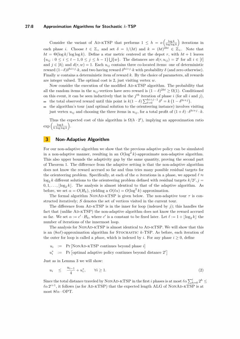
Consider the variant of Ad-kTSP that performs 1 ≤ h = o(

log klog log k

)iterations in

each phase i. Choose t ∈ Z+ and set δ = 1/(ht) and k = (ht)2ht ∈ Z+. Note thatht = Θ(log k/ log log k). Define a star metric centered at the depot r, with ht + 1 leavesuij : 0 ≤ i ≤ t − 1, 0 ≤ j ≤ h − 1

⋃w. The distances are d(r, uij) = 2i for all i ∈ [t]

and j ∈ [h]; and d(r, w) = 1. Each uij contains three co-located items: one of deterministicreward (1−δ)δhi+j ·k, and two having reward δhi+j ·k with probability δ (and zero otherwise).Finally w contains a deterministic item of reward k. By the choice of parameters, all rewardsare integer valued. The optimal cost is 2, just visiting vertex w.

Now consider the execution of the modified Ad-kTSP algorithm. The probability thatall the random items in the uij-vertices have zero reward is (1− δ)2ht ≥ Ω(1). Conditionedon this event, it can be seen inductively that in the jth iteration of phase i (for all i and j),

the total observed reward until this point is k(1− δ)∑hi+j−1`=0 δ` = k

(1− δhi+j

).

the algorithm’s tour (and optimal solution to the orienteering instance) involves visitingjust vertex uij and choosing the three items in uij , for a total profit of (1 + δ) · δhi+j · k.

Thus the expected cost of this algorithm is Ω(h · 2t), implying an approximation ratioexp

(log k

h·log log k

).

3 Non-Adaptive Algorithm

For our non-adaptive algorithm we show that the previous adaptive policy can be simulatedin a non-adaptive manner, resulting in an O(log2 k)-approximate non-adaptive algorithm.This also upper bounds the adaptivity gap by the same quantity, proving the second partof Theorem 1. The difference from the adaptive setting is that the non-adaptive algorithmdoes not know the reward accrued so far and thus tries many possible residual targets forthe orienteering problem. Specifically, at each of the α iterations in a phase, we append ` ≈log2 k different solutions to the orienteering problem defined with residual targets k/2j , j =0, 1, . . . , blog2 kc. The analysis is almost identical to that of the adaptive algorithm. Asbefore, we set α = O(Hk), yielding a O(`α) = O(log2 k) approximation.

The formal algorithm NonAd-kTSP is given below. The non-adaptive tour τ is con-structed iteratively; S denotes the set of vertices visited in the current tour.

The difference from Ad-kTSP is in the inner for loop (indexed by j); this handles thefact that (unlike Ad-kTSP) the non-adaptive algorithm does not know the reward accruedso far. We set α := c′ ·Hk, where c′ is a constant to be fixed later. Let ` := 1 + blog2 kc thenumber of iterations of the innermost loop.

The analysis for NonAd-kTSP is almost identical to Ad-kTSP. We will show that thisis an (8α`)-approximation algorithm for Stochastic k-TSP. As before, each iteration ofthe outer for loop is called a phase, which is indexed by i. For any phase i ≥ 0, define

ui := Pr [NonAd-kTSP continues beyond phase i]u∗i := Pr

[optimal adaptive policy continues beyond distance 2i

]Just as in Lemma 3 we will show:

ui ≤ ui−14 + u∗i , ∀i ≥ 1. (2)

Since the total distance traveled by NonAd-kTSP in the first i phases is at most `α∑ih=0 2h ≤

`α 2i+1, it follows (as for Ad-kTSP) that the expected length ALG of NonAd-kTSP is atmost 8`α ·OPT.

A. Ene, V. Nagarajan, and R. Saket 27:9

Algorithm 2 Algorithm NonAd-kTSP1: initialize τ, S ← ∅.2: for phase i = 0, 1, . . . do3: for t = 1, . . . , α do4: for j = 0, 1, . . . , blog2 kc do5: define profits as follows

wv :=

E[minRv, k/2j] for v ∈ V \ S0 for v ∈ S

6: using a ρ-approximation algorithm for the orienteering problem, compute a tourπ originating from r of length at most 2i with maximum total profit.

7: append tour π to τ , i.e. τ ← τ π.8: end for9: end for

10: end for

We now prove (2). Consider a fixed phase i ≥ 1 and one of the α iterations of the secondfor-loop (indexed by t). Let S denote the set of vertices visited before the start of thisiteration 〈i, t〉. Let σ denote the reward instantiations at S, and k(σ) the total reward in σ.Note that σ is only used in the analysis and not in the algorithm. Let V (i, t) ⊆ V \S be thenew vertices visited in iteration 〈i, t〉; these come from ` different subtours corresponding tothe inner for-loop. We will show (analogous to Lemma 5) that:

E

min

∑v∈V (i,t)

Rv, k − k(σ)

≥ 1

2ρ ·(

1− 1e

)· (k − k(σ))· p∗i (σ). (3)

Above, p∗i (σ) = Pr[optimal adaptive policy completes before distance 2i | σ

]. Exactly as

in the proof of Lemma 3, this would imply (2) when we set α = 8ρ ee−1 ·Hk.

It remains to prove (3). Let g ∈ 0, 1, . . . , ` denote the index such that k2g ≤ k−k(σ) <

k2g−1 and let c := k/2g. An identical proof to Lemma 4 implies:

I Lemma 9. Consider the Orienteering instance with profits sv := E[min Rv, c] forv ∈ V \ S and sv := 0 otherwise. There is an orienteering tour of length at most 2i withprofit at least c · p∗i (σ).

Let T ⊆ V \ S denote the vertices added in iteration 〈i, t〉 corresponding to inner loopiterations j ∈ 0, 1, . . . , g − 1. Note that in the inner loop iteration j = g, we haveprofits wv = E[min Rv, c] for v ∈ V \ (S ∪ T ) and wv = 0 otherwise. Lemma 9 nowimplies that the optimal profit of the orienteering instance in iteration j = g is at leastc ·p∗i (σ)−

∑u∈T E[min Ru, c]. Let T ′ denote the vertices added in the inner-loop iteration

j = g. Since we obtain a ρ-approximate solution, it follows that the additional profitobtained

∑v∈T ′ wv ≥

1ρ

(c · p∗i (σ)−

∑u∈T E[min Ru, c]

). So,

∑v∈V (i,t)

E[min Rv, c] ≥∑

v∈T∪T ′E[min Rv, c] ≥ c

ρ· p∗i (σ).

FSTTCS 2017

27:10 Approximation Algorithms for Stochastic k-TSP

Exactly as in Lemma 5 we now obtain:

E

min

∑v∈V (π)\S

Rv, c

≥ 1

ρ·(

1− 1e

)· c· p∗i (σ).

And using c ≤ k − k(σ) < 2c, we obtain (3).In the following few paragraphs we give example showing that our analysis of NonAd-

kTSP is tight, and that it is necessary for h to be Ω(log k).

3.1 Tightness of analysis of NonAd-kTSPExample 3. The analysis of NonAd-kTSP is tight up to constant factors, even in thedeterministic setting. This example is similar to that for Ad-kTSP. Consider an instanceof deterministic knapsack cover with k = 2` and `2(` + 1) items as follows. For eachi ∈ 0, 1, . . . , ` there is one item of cost 2i and reward 2i, and `2 − 1 items of cost 2i andreward 1. Clearly the optimal cost is 2`. However algorithm NonAd-kTSP will select ineach iteration i = 0, 1, . . . , ` − 3, all `2 items of cost 2i: note that the reward from theseitems is at most `3 +

∑`−3i=0 2i ≤ `3 + 2`−2 < 2`. So the algorithm’s cost is at least `2 · 2`−3,

implying an approximation ratio of Ω(log2 k).Example 4. One might also consider the variant of NonAd-kTSP where the second for-loop (indexed by t) is performed 1 ≤ h log k times instead of Θ(log k). The followingexample shows that such variants have a large approximation ratio. Consider an instance ofstochastic knapsack cover with k = 2`. There are an infinite number of items, each of cost oneand reward k with probability 2

3` (the reward is otherwise zero). For each i ∈ 0, 1, . . . , `/hand j ∈ 1, . . . , ` there are h items of cost 2i and reward k/2j with probability 2

3` (thereward is otherwise zero). The optimal (adaptive and non-adaptive) policy considers onlythe cost one items with 0, k reward, and has optimal cost O(`).

Algorithm NonAd-kTSP chooses in each iteration i ∈ 0, 1, . . . , `/h (of the first for-loop), iteration t ∈ 1, · · · , h (of the second for-loop) and iteration j ∈ 0, 1, . . . , ` (of thethird for-loop) one of the items of cost 2i with 0, k/2j reward. (This is an optimal choicefor the orienteering instance as rewards are capped at k/2j and the length bound is 2i.)These items have total cost Θ(` · 2`/h). For each j ∈ 0, 1, . . . , ` there are `

h · h = ` itemshaving reward k/2j with probability 2

3` . It can be seen that the total reward from theseitems is less than k with constant probability. So the expected cost of NonAd-kTSP isΩ(` · 2`/h), implying an approximation ratio Ω(2`/h).

4 Lower Bound on Adaptivity Gap

We show that the adaptivity gap of Stochastic k-TSP is at least e ≈ 2.718 (Theorem 2).This holds even in the special case of the stochastic covering knapsack problem with a singlerandom item. For such instances, we can even prove that the adaptivity gap is exactly e.

Here is an overview of the proof. We start by embedding an online bidding probleminto a stochastic knapsack-cover instance such that non-adaptive (adaptive) policies for thelatter correspond to online (offline) bidding strategies for the former. A result of Chrobaket al. [13] shows that no online bidding strategy is better than e-competitive. To completethe analysis, LP duality is used to show that the worst possible adaptivity gap for thestochastic knapsack-cover instance equals the best possible competitiveness of any onlinebidding strategy.

The gap example is based on the following problem studied in [13].

A. Ene, V. Nagarajan, and R. Saket 27:11

I Definition 10 (Online Bidding Problem). Given input n ∈ Z+, an algorithm outputs arandomized sequence b1, b2, . . . , b` of bids from the set [n] := 1, 2, . . . , n. The algorithm’scost under (an unknown) threshold T ∈ [n] equals the (expected) sum of its bid values untilit bids a value at least T . The algorithm is β-competitive if its cost under threshold T is atmost β · T , for all T ∈ [n].

I Theorem 11 ([13]). There is no randomized algorithm for online bidding that is less thane-competitive.

Without loss of generality, any bid sequence must be increasing; let Γ denote the setof increasing sequences on [n]. For any I ∈ Γ and T ∈ [n], let C(I, T ) denote the cost ofsequence I under threshold T . In terms of this notation, Theorem 11 is equivalent to:

minπ :distribution(Γ)

maxT∈[n]

EI←π[C(I, T )]T

≥ e. (4)

We now define the stochastic covering knapsack instance. The target k := 2n+1. Thereis one random item r of zero cost having reward k − 2i with probability pi (for all i ∈ [n]).There are n deterministic items uini=1 where ui has cost i and reward 2i. We will showthat there exist probabilities pis so that the adaptivity gap is e.

It is clear that an optimal policy (adaptive or non-adaptive) will first choose item r,since it has zero cost. Moreover, an optimal adaptive policy will next choose item ui exactlywhen r is observed to have reward k − 2i. Hence the optimal adaptive cost is

∑ni=1 i · pi.

Any non-adaptive policy is given by a sequence τ of the deterministic items; recall thatitem r is always chosen first. Moreover, due to the exponentially increasing rewards, we canassume that τ is an increasing sub-sequence of ui : 1 ≤ i ≤ n. So there is a one-to-onecorrespondence between non-adaptive policies and Γ (in the online bidding instance). Notethat the cost of non-adaptive solution I ∈ Γ is exactly

∑nT=1 pT · C(I, T ); if the random

item r has size k− 2T then the policy will keep choosing items in I until it reaches an indexat least T . Thus, the maximum adaptivity gap achieved by such an instance is:

maxp :distribution([n])

minI∈Γ

ET←p[C(I, T )]ET←p[T ] . (5)

The next lemma relates the quantities in (4) and (5). Below, for any set S, D(S) denotesthe collection of probability distributions on S.

I Lemma 12. For any non-negative matrix C(Γ, [n]), we have:

maxp∈D([n])

minI∈Γ

ET←p[C(I, T )]ET←p[T ] = min

π∈D(Γ)maxT∈[n]

EI←π[C(I, T )]T

.

Proof. The second expression equals the LP:

min β

s.t. T · β −∑I∈Γ C(I, T ) · π(I) ≥ 0, ∀T ∈ [n],∑

I∈Γ π(I) ≥ 1,β, π ≥ 0.

Taking the dual, we obtain:

max α

s.t. α−∑T∈[n] C(I, T ) · σ(T ) ≤ 0, ∀I ∈ Γ,∑

T∈[n] T · σ(I) ≤ 1,α, σ ≥ 0.

FSTTCS 2017

27:12 Approximation Algorithms for Stochastic k-TSP

Define functions g, f : [n]→ R+ where

f(p) := minI∈Γ

n∑T=1

pT · C(I, T ) and g(p) :=n∑

T=1pT · T.

Note that when p corresponds to a probability distribution, f(p) = minI∈Γ ET←p[C(I, T )]and g(p) = ET←p[T ]. So the first expression in the lemma is just maxp∈D([n]) f(p)/g(p). Thekey observation is that f and g are homogeneous, i.e. f(a ·p) = a ·f(p) and g(a ·p) = a ·g(p)for any scalar a ∈ R+ and vector p ∈ Rn+. This implies that the first expression equals:

maxp∈D([n])

f(p)g(p) = max

p∈Rn+

f(p)g(p) = max

p∈Rn+ : g(p)≤1

f(p).

It is easy to check that this equals the dual LP above, which proves the lemma. J

Thus the above instance of stochastic knapsack cover has adaptivity gap at least e, whichproves Theorem 2. It can also be shown that every instance of stochastic knapsack cover witha single stochastic item has adaptivity gap at most e: this uses a relation to the incrementalk-MST problem [29].

I Proposition 13. The adaptivity gap of any instance of stochastic knapsack cover with asingle random item is at most e.

Proof. Consider any such instance with item n having random reward R ∈ 0, 1, · · · k andeach item i ∈ [n− 1] having deterministic reward ri. Let ci denote the cost of each i ∈ [n].As there is only one random item, any adaptive policy is of the following form (i) select asubset T1 ⊆ [n− 1] of deterministic items, (ii) select random item n, (iii) depending on thevalue of reward R, select subset T2(R) ⊆ [n− 1] of deterministic items.

Note that if the reward in T1 is itself at least k then we do not even need to use therandom item: so the optimal adaptive and non-adaptive policies are the same (both are T1).On the other hand, if r(T1) < k then the random item will be selected with probability one:so we can assume that it is the first item to be selected, i.e. T1 = ∅.

Now, consider the following incremental k-MST instance. There are n vertices withdistances induced by a star with root n and leaves [n − 1] where the distance d(n, i) = ci.There is zero reward at the root and reward ri at each i ∈ [n − 1]. The goal is to find arandom sequence σ of edges so that the following ratio is minimized:

max`≥0

Eσ[cost of minimal prefix of σ with reward at least `]optimal `-MST value .

As shown in [29], there is always a random sequence σ with the above ratio at most e.In the stochastic knapsack-cover instance let p` = Pr[R = `] for ` ∈ 0, 1, · · · k. Then

it is clear that the adaptive optimum is AD = cn +∑k`=0 pk−` · OPT (`) where OPT (`)

is the optimal `-MST value. Note also that the sequence σ corresponds to a randomizednon-adaptive solution: item n followed by the remaining n− 1 items in the order that theyfirst appear in σ. This has expected value NA = cn +

∑k`=0 pk−` ·Eσ[σ(`)] where σ(`) is the

cost of the minimal prefix of σ with reward at least `. So the adaptivity gap is at most:

NA

AD=cn +

∑k`=0 pk−` · Eσ[σ(`)]

cn +∑k`=0 pk−` ·OPT (`)

≤ max`

Eσ[σ(`)]OPT (`) ≤ e.

This also implies that the best deterministic non-adaptive policy costs at most e ·AD. J

A. Ene, V. Nagarajan, and R. Saket 27:13

5 Conclusion

The main (perhaps challenging) open question is to obtain a constant-factor approximationalgorithm for Stochastic k-TSP in either the adaptive or non-adaptive setting. Anotherinteresting question is the adaptivity gap, even in the special case of stochastic knapsackcover, where there is a wide gap between the lower bound of e and upper bound of O(log2 k).

Acknowledgment

We thank Itai Ashlagi for initial discussions that lead to this problem definition.

References1 M. Adamczyk. Improved analysis of the greedy algorithm for stochastic matching. Infor-

mation Processing Letters, 111(15):731–737, 2011.2 M. Adamczyk, F. Grandoni, and J. Mukherjee. Improved approximation algorithms for

stochastic matching. In Proc. Annual European Symposium on Algorithms, pages 1–12,2015.

3 M. Adamczyk, M. Sviridenko, and J. Ward. Submodular stochastic probing on matroids.Math. Oper. Res., 41(3):1022–1038, 2016.

4 Y. Azar, A. Madry, T. Moscibroda, D. Panigrahi, and A. Srinivasan. Maximum bipartiteflow in networks with adaptive channel width. Theoretical Computer Science, 412(24):2577–2587, 2011.

5 N. Bansal, A. Gupta, J. Li, J. Mestre, V. Nagarajan, and A. Rudra. When LP is thecure for your matching woes: Improved bounds for stochastic matchings. Algorithmica,63(4):733–762, 2012.

6 N. Bansal and V. Nagarajan. On the adaptivity gap of stochastic orienteering. MathematicalProgramming, 154(1-2):145–172, 2015.

7 A. Baveja, A. Chavan, A. Nikiforov, A. Srinivasan, and P. Xu. Improved bounds in stochas-tic matching and optimization. In Proc. International Workshop on Approximation Algo-rithms for Combinatorial Optimization Problems (APPROX), pages 124–134, 2015.

8 A. Bhalgat, A. Goel, and S. Khanna. Improved approximation results for stochastic knap-sack problems. In Proc. Annual ACM-SIAM Symposium on Discrete Algorithms, pages1647–1665. Society for Industrial and Applied Mathematics, 2011.

9 A. Blum, S. Chawla, D. R. Karger, T. Lane, A. Meyerson, and M. Minkoff. Approximationalgorithms for orienteering and discounted-reward TSP. SIAM Journal of Computing,37(2):653–670, 2007.

10 K. Chaudhuri, B. Godfrey, S. Rao, and K. Talwar. Paths, trees, and minimum latencytours. In Proc. Annual Symposium on Foundations of Computer Science, pages 36–45,2003.

11 C. Chekuri, N. Korula, and M. Pál. Improved algorithms for orienteering and relatedproblems. ACM Transactions on Algorithms, 8(3):23, 2012.

12 N. Chen, N. Immorlica, A. R Karlin, M. Mahdian, and A. Rudra. Approximating matchesmade in heaven. In Proc. International Colloquium on Automata, Languages and Program-ming, pages 266–278. Springer, 2009.

13 M. Chrobak, C. Kenyon, J. Noga, and N. E. Young. Incremental medians via online bidding.Algorithmica, 50(4):455–478, 2008.

14 B. C Dean, M. X. Goemans, and J. Vondrák. Adaptivity and approximation for stochasticpacking problems. In Proc. Annual ACM-SIAM Symposium on Discrete Algorithms, pages395–404. Society for Industrial and Applied Mathematics, 2005.

FSTTCS 2017

27:14 Approximation Algorithms for Stochastic k-TSP

15 B. C. Dean, M. X. Goemans, and J. Vondrák. Approximating the stochastic knapsackproblem: The benefit of adaptivity. Math. Oper. Res., 33(4):945–964, 2008.

16 A. Deshpande, L. Hellerstein, and D. Kletenik. Approximation algorithms for stochasticsubmodular set cover with applications to boolean function evaluation and min-knapsack.ACM Transactions on Algorithms, 12(3):42, 2016.

17 J. Fakcharoenphol, C. Harrelson, and S. Rao. The k-traveling repairmen problem. ACMTransactions on Algorithms, 3(4), 2007.

18 N. Garg. Saving an epsilon: a 2-approximation for the k-mst problem in graphs. In Proc.ACM Symposium on the Theory of Computing, pages 396–402, 2005.

19 M. X. Goemans and Jan Vondrák. Stochastic covering and adaptivity. In Proc. LatinAmerican Symposium on Theoretical Informatics(LATIN), pages 532–543, 2006.

20 D. Golovin and A. Krause. Adaptive submodularity: Theory and applications in activelearning and stochastic optimization. Journal of Artificial Intelligence Research, 42:427–486, 2011.

21 N. Grammel, L. Hellerstein, D. Kletenik, and P. Lin. Scenario submodular cover. InInternational Workshop on Approximation and Online Algorithms, pages 116–128. Springer,2016.

22 S. Guha and K. Munagala. Multi-armed bandits with metric switching costs. Automata,Languages and Programming, pages 496–507, 2009.

23 A. Gupta, R. Krishnaswamy, M. Molinaro, and R. Ravi. Approximation algorithms for cor-related knapsacks and non-martingale bandits. In Proc. Annual Symposium on Foundationsof Computer Science, pages 827–836, 2011.

24 A. Gupta, R. Krishnaswamy, V. Nagarajan, and R. Ravi. Running errands in time: Ap-proximation algorithms for stochastic orienteering. Math. Oper. Res., 40(1):56–79, 2015.

25 A. Gupta and V. Nagarajan. A stochastic probing problem with applications. In Proc.Conference on Integer Programming and Combinatorial Optimization (IPCO), pages 205–216, 2013.

26 A. Gupta, V. Nagarajan, and S. Singla. Adaptivity gaps for stochastic probing: Submodularand XOS functions. In Proc. Annual ACM-SIAM Symposium on Discrete Algorithms, pages1688–1702, 2017.

27 Sungjin Im, Viswanath Nagarajan, and Ruben van der Zwaan. Minimum latency submod-ular cover. ACM Trans. Algorithms, 13(1):13:1–13:28, 2016.

28 P. Kambadur, V. Nagarajan, and F. Navidi. Adaptive submodular ranking. In Proc.Conference on Integer Programming and Combinatorial Optimization (IPCO), pages 317–329, 2017.

29 G. Lin, C. Nagarajan, R. Rajaraman, and D. P. Williamson. A general approach forincremental approximation and hierarchical clustering. SIAM Journal of Computing,39(8):3633–3669, 2010.

30 W. Ma. Improvements and generalizations of stochastic knapsack and multi-armed banditapproximation algorithms. In Proc. Annual ACM-SIAM Symposium on Discrete Algo-rithms, pages 1154–1163. Society for Industrial and Applied Mathematics, 2014.