Applications of Wavelets inNumerical Mathematics

Kees Verhoeven

1. Brief summary

2. Data compression

3. Denoising

4. Preconditioning

5. Adaptive grids

6. Integral equations

1

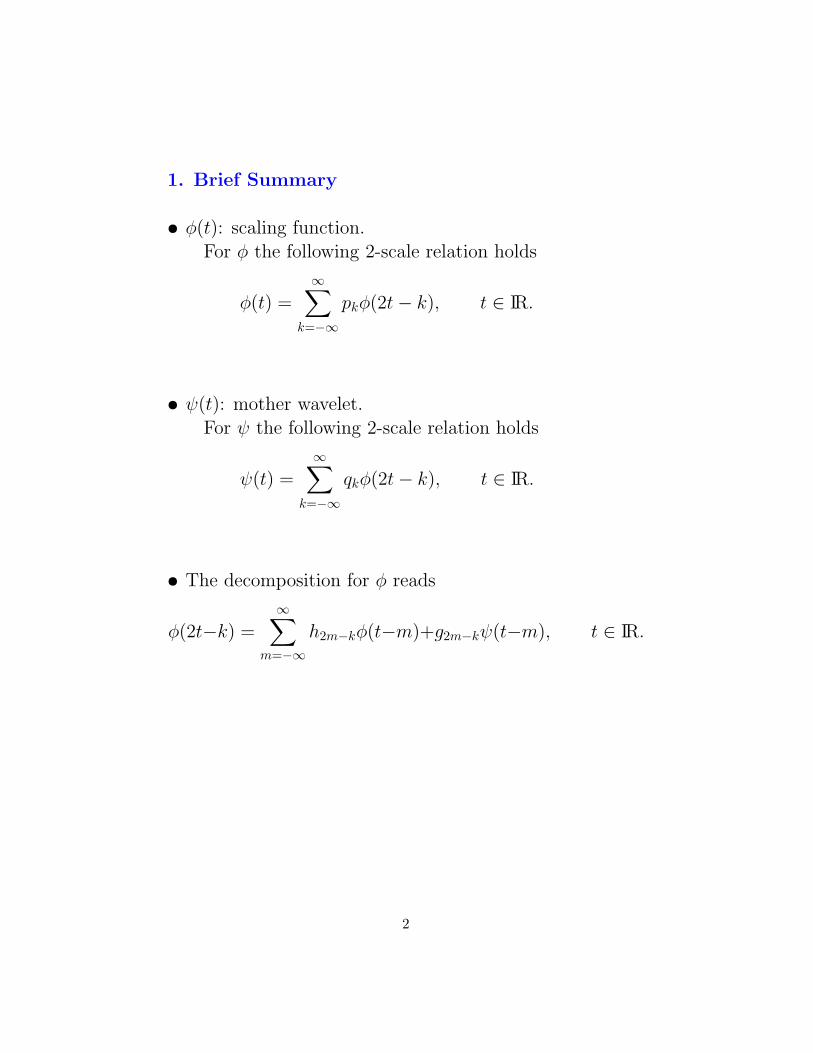
1. Brief Summary

• φ(t): scaling function.For φ the following 2-scale relation holds

φ(t) =∞∑

k=−∞

pkφ(2t− k), t ∈ IR.

• ψ(t): mother wavelet.For ψ the following 2-scale relation holds

ψ(t) =∞∑

k=−∞

qkφ(2t− k), t ∈ IR.

• The decomposition for φ reads

φ(2t−k) =∞∑

m=−∞h2m−kφ(t−m)+g2m−kψ(t−m), t ∈ IR.

2

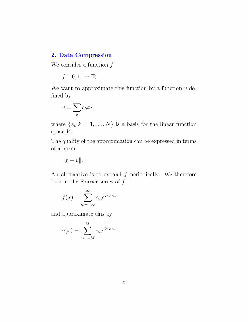
2. Data Compression

We consider a function f

f : [0, 1]→ IR.

We want to approximate this function by a function v de-fined by

v =∑k

ckφk,

where φk|k = 1, . . . , N is a basis for the linear functionspace V .

The quality of the approximation can be expressed in termsof a norm

‖f − v‖.

An alternative is to expand f periodically. We thereforelook at the Fourier series of f

f(x) =∞∑

m=−∞cme

2πimx

and approximate this by

v(x) =M∑

m=−M

cme2πimx.

3

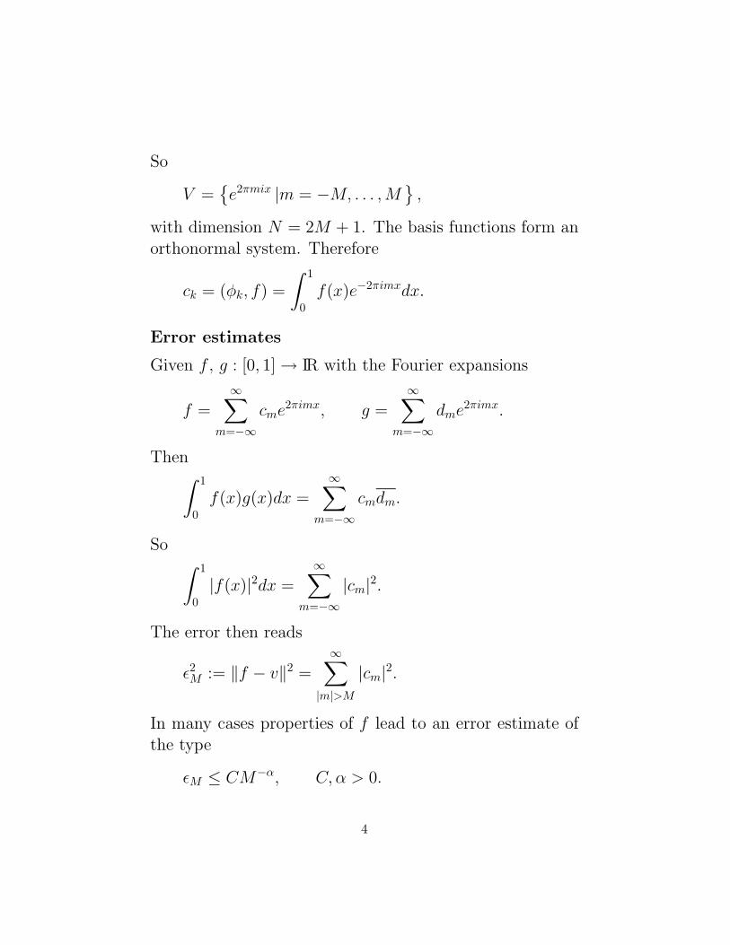
So

V =e2πmix |m = −M, . . . ,M

,

with dimension N = 2M + 1. The basis functions form anorthonormal system. Therefore

ck = (φk, f) =

∫ 1

0f(x)e−2πimxdx.

Error estimates

Given f , g : [0, 1]→ IR with the Fourier expansions

f =∞∑

m=−∞cme

2πimx, g =∞∑

m=−∞dme

2πimx.

Then∫ 1

0f(x)g(x)dx =

∞∑m=−∞

cmdm.

So ∫ 1

0|f(x)|2dx =

∞∑m=−∞

|cm|2.

The error then reads

ε2M := ‖f − v‖2 =∞∑

|m|>M

|cm|2.

In many cases properties of f lead to an error estimate ofthe type

εM ≤ CM−α, C, α > 0.

4

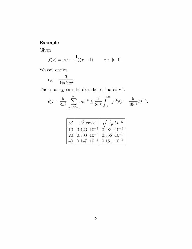
Example

Given

f(x) = x(x− 1

2)(x− 1), x ∈ [0, 1].

We can derive

cm =3

4iπ3m3 .

The error εM can therefore be estimated via

ε2M =9

8π6

∞∑m=M+1

m−6 ≤ 9

8π6

∫ ∞M

y−6dy =9

40π6M−5.

M L2-error√

940π6M−5

10 0.426 ·10−4 0.484 ·10−4

20 0.803 ·10−5 0.855 ·10−5

40 0.147 ·10−5 0.151 ·10−5

5

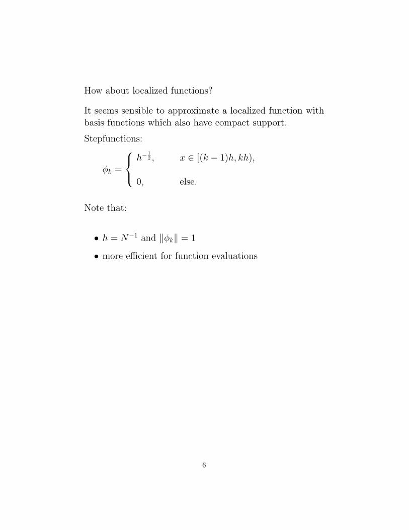
How about localized functions?

It seems sensible to approximate a localized function withbasis functions which also have compact support.

Stepfunctions:

φk =

h−12 , x ∈ [(k − 1)h, kh),

0, else.

Note that:

• h = N−1 and ‖φk‖ = 1

• more efficient for function evaluations

6

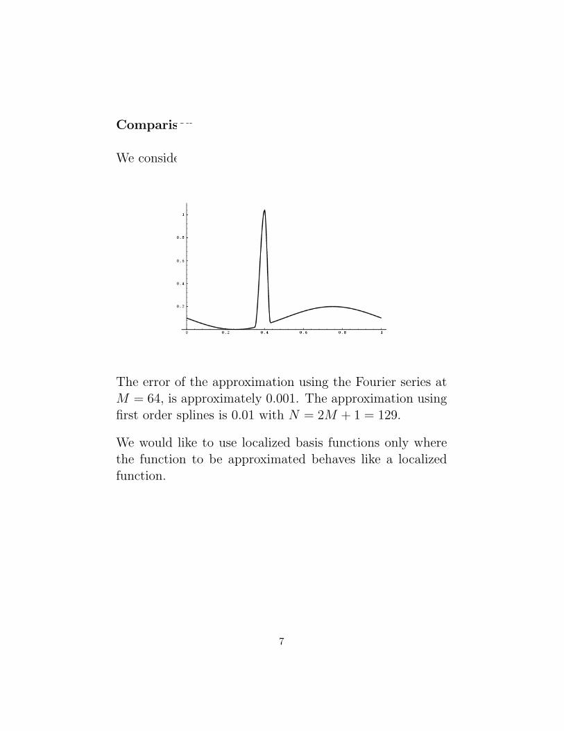
Comparison

We consider the following function.

The error of the approximation using the Fourier series atM = 64, is approximately 0.001. The approximation usingfirst order splines is 0.01 with N = 2M + 1 = 129.

We would like to use localized basis functions only wherethe function to be approximated behaves like a localizedfunction.

7

Therefore, we would like basis functions which all have thesame shape but different scales. Then, if we have

v =N∑k=1

ckφk

and |cj| ε, we also have∥∥∥∥∥f −∑k

ckφk

∥∥∥∥∥ ≤∥∥∥∥∥∥f −

∑k 6=j

ckφk

∥∥∥∥∥∥+ ‖cjφj‖.

This leads to data compression.

8

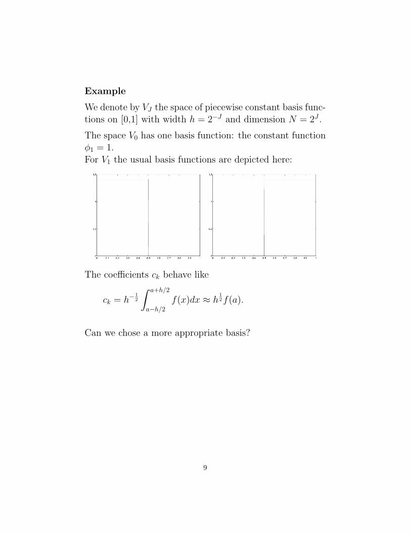
Example

We denote by VJ the space of piecewise constant basis func-tions on [0,1] with width h = 2−J and dimension N = 2J .

The space V0 has one basis function: the constant functionφ1 = 1.For V1 the usual basis functions are depicted here:

The coefficients ck behave like

ck = h−12

∫ a+h/2

a−h/2f(x)dx ≈ h

12f(a).

Can we chose a more appropriate basis?

9

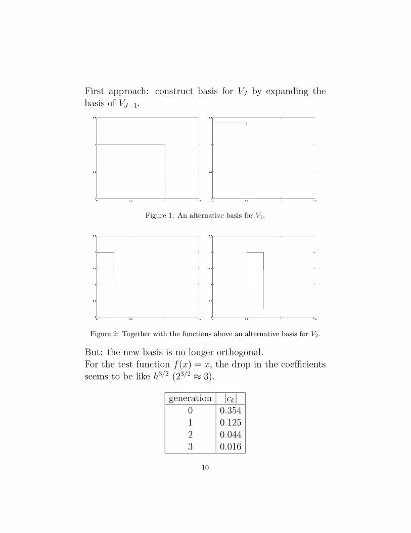
First approach: construct basis for VJ by expanding thebasis of VJ−1.

Figure 1: An alternative basis for V1.

Figure 2: Together with the functions above an alternative basis for V2.

But: the new basis is no longer orthogonal.For the test function f(x) = x, the drop in the coefficientsseems to be like h3/2 (23/2 ≈ 3).

generation |ck|0 0.3541 0.1252 0.0443 0.016

10

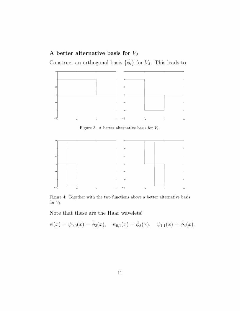
A better alternative basis for VJ

Construct an orthogonal basis φi for VJ . This leads to

Figure 3: A better alternative basis for V1.

Figure 4: Together with the two functions above a better alternative basisfor V2.

Note that these are the Haar wavelets!

ψ(x) = ψ0,0(x) = φ2(x), ψ0,1(x) = φ3(x), ψ1,1(x) = φ4(x).

11

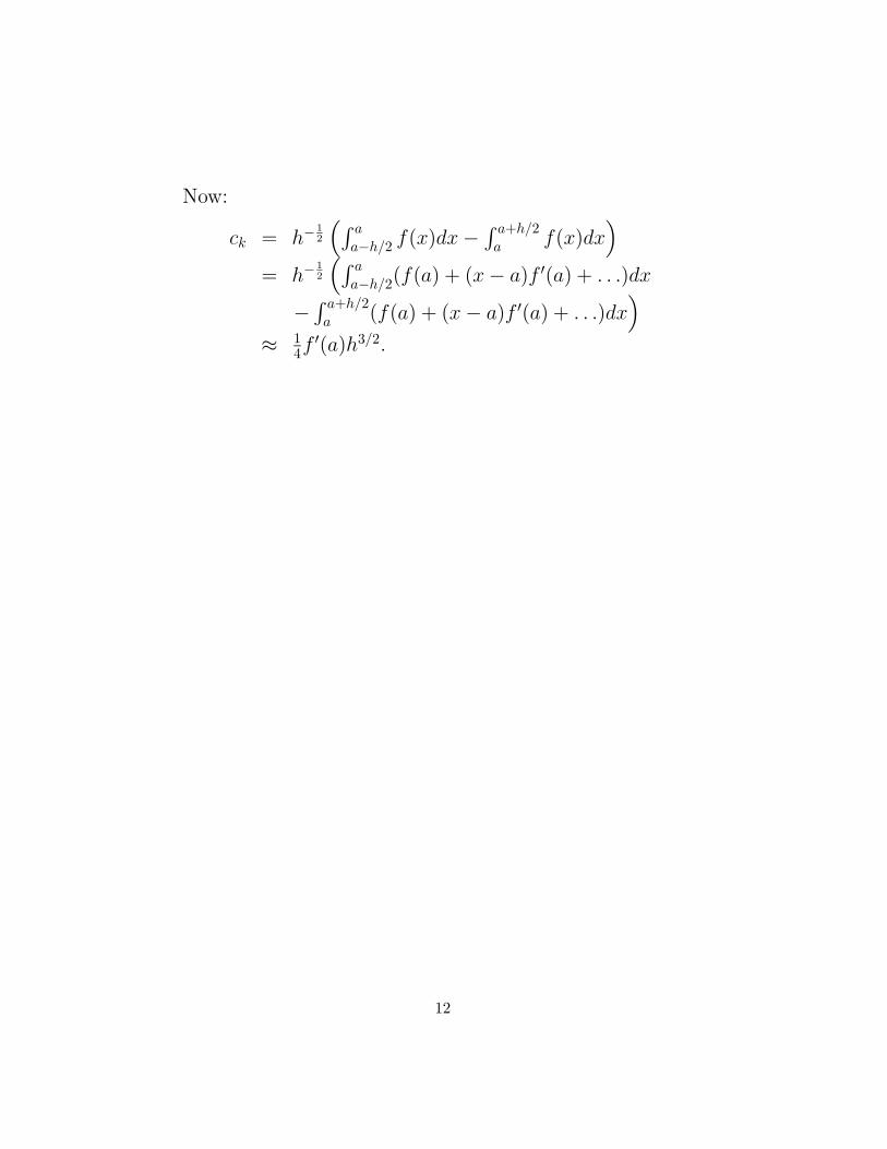
Now:

ck = h−12

(∫ aa−h/2 f(x)dx−

∫ a+h/2a f(x)dx

)= h−

12

(∫ aa−h/2(f(a) + (x− a)f ′(a) + . . .)dx

−∫ a+h/2a (f(a) + (x− a)f ′(a) + . . .)dx

)≈ 1

4f′(a)h3/2.

12

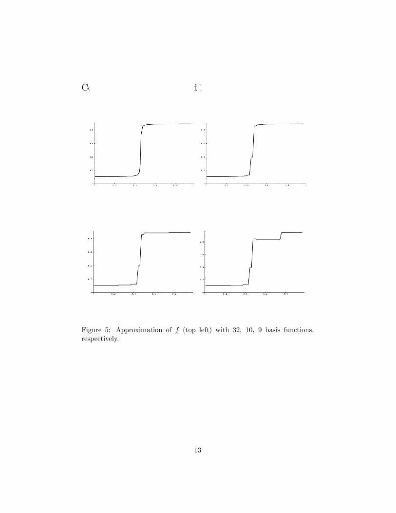
Comparison of this basis and homogeneous one:

Figure 5: Approximation of f (top left) with 32, 10, 9 basis functions,respectively.

13

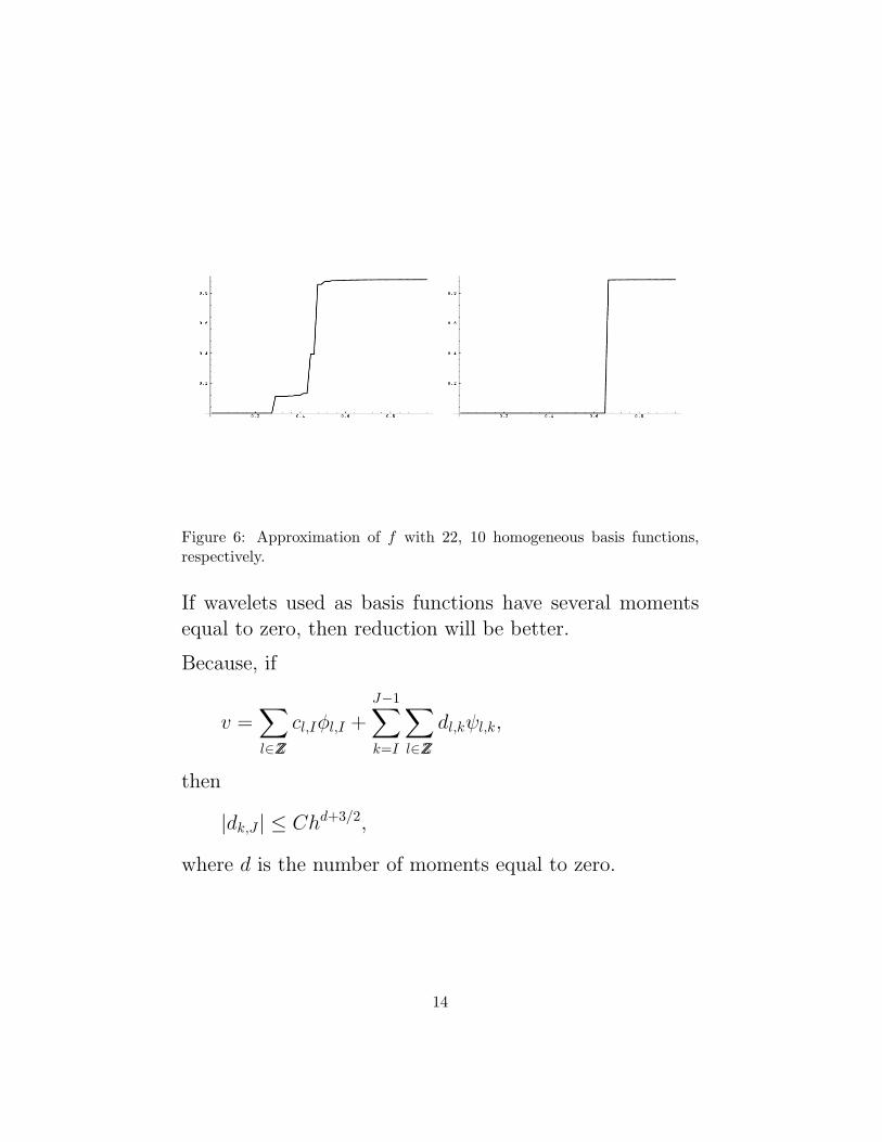
Figure 6: Approximation of f with 22, 10 homogeneous basis functions,respectively.

If wavelets used as basis functions have several momentsequal to zero, then reduction will be better.

Because, if

v =∑l∈ZZ

cl,Iφl,I +J−1∑k=I

∑l∈ZZ

dl,kψl,k,

then

|dk,J | ≤ Chd+3/2,

where d is the number of moments equal to zero.

14

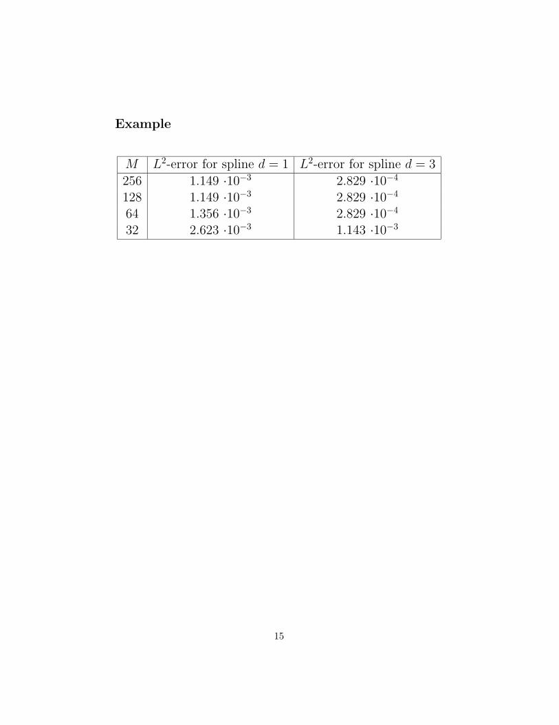
Example

M L2-error for spline d = 1 L2-error for spline d = 3

256 1.149 ·10−3 2.829 ·10−4

128 1.149 ·10−3 2.829 ·10−4

64 1.356 ·10−3 2.829 ·10−4

32 2.623 ·10−3 1.143 ·10−3

15

3. Denoising

Suppose we have a signal with some noise. We can make awavelet decomposition up to a certain depth.If the coefficients of the wavelets remain relatively large(say |dj, k| > ε), then we have some localized noise.So cancel these contributions by forcing dj,k = 0 at L levelsdeep.

Then, we can reconstruct the filtered signal.

16

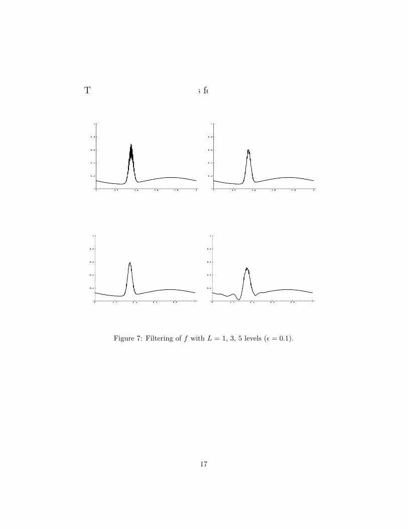
The role of L can be seen as follows:

Figure 7: Filtering of f with L = 1, 3, 5 levels (ε = 0.1).

17

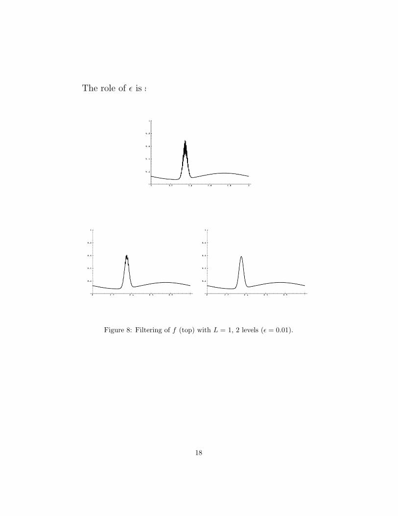
The role of ε is shown here:

Figure 8: Filtering of f (top) with L = 1, 2 levels (ε = 0.01).

18

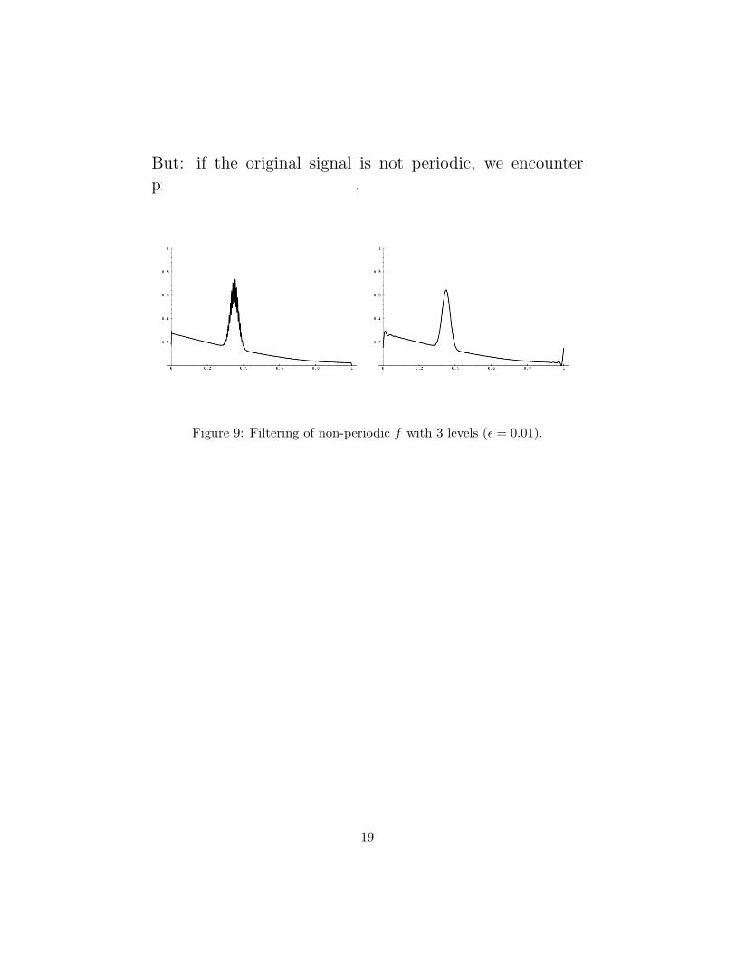
But: if the original signal is not periodic, we encounterproblems at the boundaries.

Figure 9: Filtering of non-periodic f with 3 levels (ε = 0.01).

19

4. Preconditioning

Consider

D(u) = f

on a domain Ω, with the differential operator D elliptic. IfD is linear, this would lead to a linear system

Dc = r,

with

Dj,k = (φj,Dφk), rj = (φj, f).

The matrix D is called the stiffness matrix. If we use aniterative method to solve this system, the speed of con-vergence strongly depends on the condition number of thematrix D, κ(D) = ‖D‖‖D−1‖, with

‖D‖ = sup‖c‖=1

cTDc, ‖D−1‖−1 = inf‖c‖=1

cTDc.

For symmetric matrices, we can express the condition num-ber in terms of the eigenvalues:

κ(D) =λmax

λmin.

20

Example

We consider

D(u) = −d2u

dx2 + u = f, x ∈ (0, 1),

with periodical boundary conditions.We assume that the numerical solution v can be writtenas a linear combination of certain scaling functions whichspan VJ .Galerkin’s method and integration by parts gives us

Dc = r,

with

Di,j =

(dφi,Jdx

,dφj,Jdx

)+ (φi,J , φj,J),

and, as before

rj = (φj, f).

For linear B-splines:(dφi,Jdx

,dφj,Jdx

)=

∫2J/2

d

dxφ(2Jx−i)2J/2 d

dxφ(2Jx−j)dx.

The derivatives are piecewise constant, and therefore wederive

Di,j =

2N 2 + 2

3 , i = j,

−N 2 + 16 , i = (j ± 1) mod N,

0 else.

This is a circulant matrix, that is Di,j = d(i− j).

21

We define the symbol of a circulant matrix as

D(z) =∑j

Di,jzi−j.

For D now follows

λmax = maxzN=1|D(z)|, λmin = min

zN=1|D(z)|.

For the differential equation we have

D(z) =∑j

((dφi,Jdx

,dφj,Jdx

)+ (φi,J , φj,J)

)zi−j.

We write

D(z) = D1(z) +D2(z),

with

D1(z) =∑j

(dφi,Jdx

,dφj,Jdx

)zi−j, D2(z) =

∑j

(φi,J , φj,J)zi−j.

The second term can be recognized as D2(z) = Rφ(z). Inthe same manner we can derive D1(z) = 22JRφ(z).Using this and the 2-scale relations, we can derive

D(z) = N 2(2− z − z−1) +1

6(4 + z + z−1).

Calculating the biggest and smallest eigenvalue, we see that

κ1 = 4N 2 +1

3.

If N →∞, κ1 →∞.

22

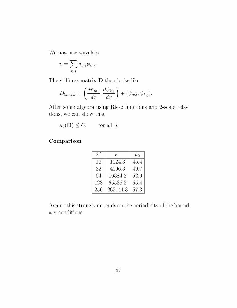
We now use wavelets

v =∑k,j

dk,jψk,j.

The stiffness matrix D then looks like

Dl,m,j,k =

(dψm,ldx

,dψk,jdx

)+ (ψm,l, ψk,j).

After some algebra using Riesz functions and 2-scale rela-tions, we can show that

κ2(D) ≤ C, for all J.

Comparison

2J κ1 κ2

16 1024.3 45.432 4096.3 49.764 16384.3 52.9128 65536.3 55.4256 262144.3 57.3

Again: this strongly depends on the periodicity of the bound-ary conditions.

23

5. Adaptive grids

We consider a hyperbolic PDE

∂u(x, t)

∂t= F(u,

∂u

∂x, . . .),

together with initial condition and periodic boundary con-ditions.

The approximation of the initial condition u(x, 0) is doneby

v(x, 0) =N−1∑i=0

ci,I(0)φi,I(x) +J−1∑j=I

∑i∈Ij

di,j(0)ψi,j(x).

Here N = 2J is the amount of intervals on the coarsestgrid I, the set Ij is a subset of all possible wavelets on thegrids j = I, . . . , J −1. These sets Ij are found by making awavelet decomposition and leave out all wavelet coefficientsbelow a certain threshold ε.

But: this would mean that we have to approximate thefunction on the finest grid first!

24

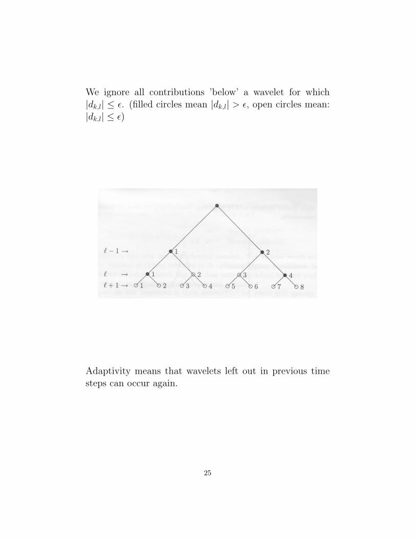
We ignore all contributions ’below’ a wavelet for which|dk,l| ≤ ε. (filled circles mean |dk,l| > ε, open circles mean:|dk,l| ≤ ε)

Adaptivity means that wavelets left out in previous timesteps can occur again.

25

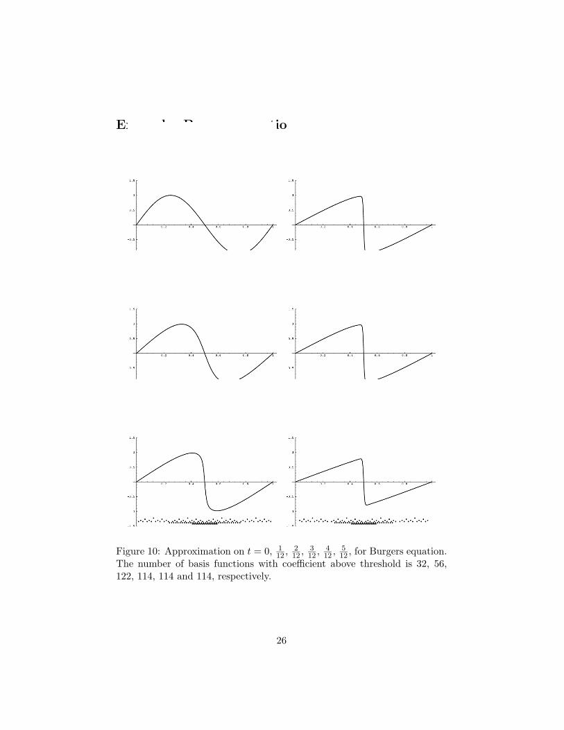
Example: Burgers equation

Figure 10: Approximation on t = 0, 112 , 2

12 , 312 , 4

12 , 512 , for Burgers equation.

The number of basis functions with coefficient above threshold is 32, 56,122, 114, 114 and 114, respectively.

26

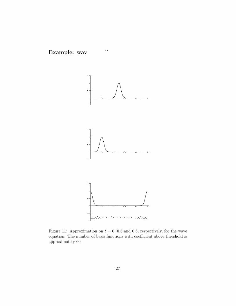
Example: wave equation

Figure 11: Approximation on t = 0, 0.3 and 0.5, respectively, for the waveequation. The number of basis functions with coefficient above threshold isapproximately 60.

27

6. Integral Equations

We consider

u(x) =

∫K(x; t)u(t)dt+ f(x).

We take

v(x) =∑j

cjφj(x).

Galerkin’s method would leave us with

Ac = r,

with

Aj,k = (φj, φk)−∫ ∫

φj(x)K(x; t)φk(t)dxdt, rj = (φj, f).

Often this A is well conditioned, but full.

Using wavelets reduces the number of nonzero elements.We represent

v(x) =∑l∈ZZ

cl,Iφl,I +J−1∑k=I

∑l∈ZZ

dl,kψl,k.

Look at the second term of A

Kl,m,j,k =

∫ ∫ψm,l(x)K(x; t)ψk,j(t)dxdt.

We make the following assumption on K(x; t)∣∣∣∣ ∂d∂xdK(x; t)

∣∣∣∣+

∣∣∣∣ ∂d∂tdK(x; t)

∣∣∣∣ ≤ Cd1

|x− t|d+1 ,

for a certain d > 0.

28

Making use of the Taylor series of K(x; t) and taking awavelet with d zero moments, we can derive

|Kl,m,j,k| ≤ C1

|x0 − t0|d+1 .

Using this we can bring down the number of nonzero ele-ments (or better: the number of elements with value abovea certain threshold ε).

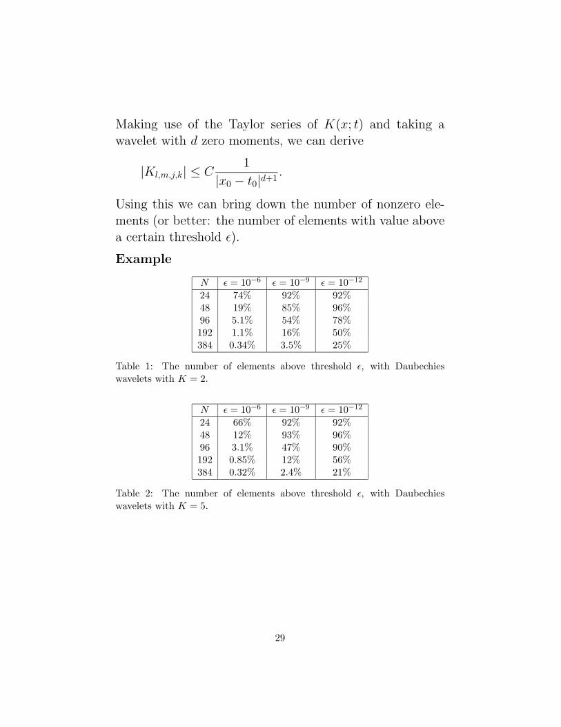
Example

N ε = 10−6 ε = 10−9 ε = 10−12

24 74% 92% 92%48 19% 85% 96%96 5.1% 54% 78%192 1.1% 16% 50%384 0.34% 3.5% 25%

Table 1: The number of elements above threshold ε, with Daubechieswavelets with K = 2.

N ε = 10−6 ε = 10−9 ε = 10−12

24 66% 92% 92%48 12% 93% 96%96 3.1% 47% 90%192 0.85% 12% 56%384 0.32% 2.4% 21%

Table 2: The number of elements above threshold ε, with Daubechieswavelets with K = 5.

29