Appendix S5 Solutions to Chapter 5 exercisespeople.ucalgary.ca/~lvov/543/chap5soln.pdf · S5...
34
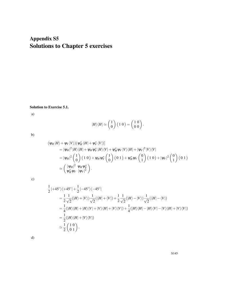
Appendix S5 Solutions to Chapter 5 exercises Solution to Exercise 5.1. a) |HihH|’ 1 0 ( 10 ) = 10 00 . b) (ψ H |Hi + ψ V | V i)(ψ * H hH| + ψ * V h V |)] = |ψ H | 2 |HihH| + ψ H ψ * V |Hih V | + ψ * H ψ V | V ihH| + |ψ V | 2 | V ih V | = |ψ H | 2 1 0 ( 10 ) + ψ H ψ * V 1 0 ( 01 ) + ψ * H ψ V 0 1 ( 10 ) + |ψ V | 2 0 1 ( 01 ) ’ |ψ H | 2 ψ H ψ * V ψ * H ψ V |ψ V | 2 . c) 1 2 |+45 ◦ ih+45 ◦ | + 1 2 |-45 ◦ ih-45 ◦ | = 1 2 1 √ 2 (|Hi + | V i) 1 √ 2 (hH| + h V |)+ 1 2 1 √ 2 (|Hi-| V i) 1 √ 2 (hH|-h V |) = 1 4 (|HihH| + |Hih V | + | V ihH| + | V ih V |)+ 1 4 (|HihH|-|Hih V |-| V ihH| + | V ih V |) = 1 2 (|HihH| + | V ih V |) ’ 1 2 10 01 . d) S145
Transcript of Appendix S5 Solutions to Chapter 5 exercisespeople.ucalgary.ca/~lvov/543/chap5soln.pdf · S5...
Appendix S5Solutions to Chapter 5 exercises
Solution to Exercise 5.1.
a)
|H〉〈H| '(
10
)(1 0)=
(1 00 0
).
b)
(ψH |H〉+ψV |V 〉)(ψ∗H 〈H|+ψ∗V 〈V |)]
= |ψH |2 |H〉〈H|+ψHψ∗V |H〉〈V |+ψ
∗HψV |V 〉〈H|+ |ψV |2 |V 〉〈V |
= |ψH |2(
10
)(1 0)+ψHψ
∗V
(10
)(0 1)+ψ
∗HψV
(01
)(1 0)+ |ψV |2
(01
)(0 1)
'(|ψH |2 ψHψ∗Vψ∗HψV |ψV |2
).
c)
12|+45〉〈+45|+ 1
2|−45〉〈−45|
=12
1√2(|H〉+ |V 〉) 1√
2(〈H|+ 〈V |)+ 1
21√2(|H〉− |V 〉) 1√
2(〈H|− 〈V |)
=14(|H〉〈H|+ |H〉〈V |+ |V 〉〈H|+ |V 〉〈V |)+ 1
4(|H〉〈H|− |H〉〈V |− |V 〉〈H|+ |V 〉〈V |)
=12(|H〉〈H|+ |V 〉〈V |)
' 12
(1 00 1
).
d)
S145
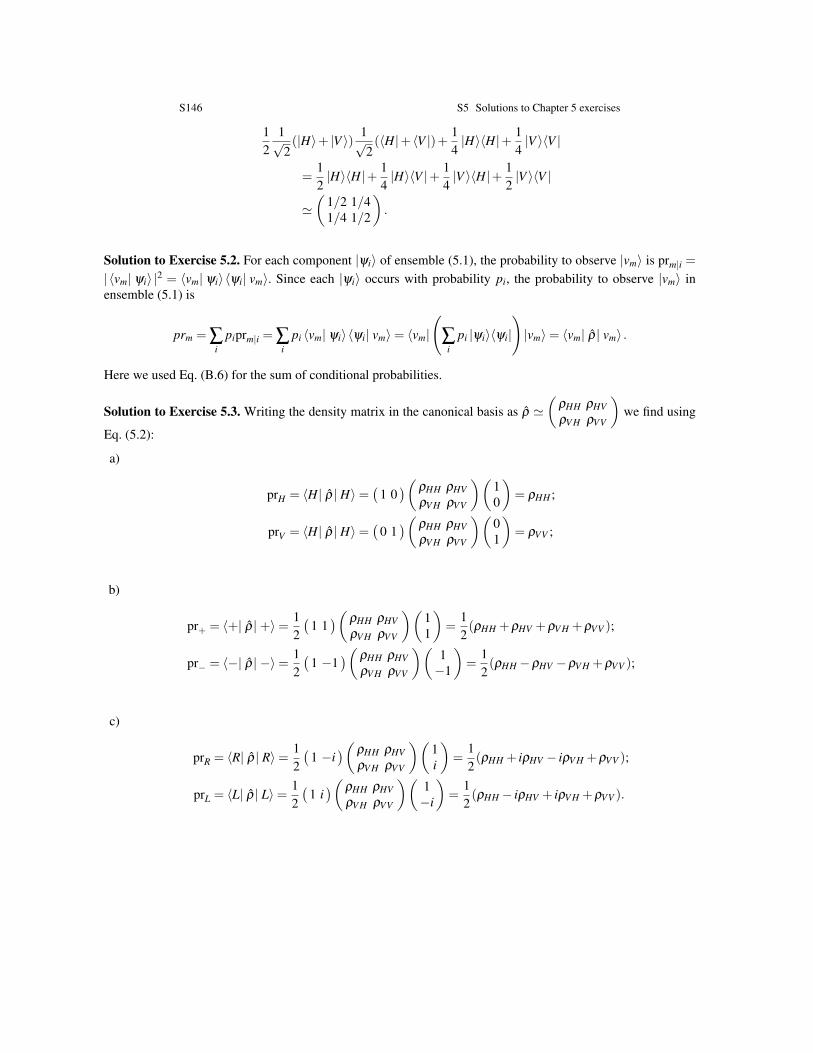
S146 S5 Solutions to Chapter 5 exercises
12
1√2(|H〉+ |V 〉) 1√
2(〈H|+ 〈V |)+ 1
4|H〉〈H|+ 1
4|V 〉〈V |
=12|H〉〈H|+ 1
4|H〉〈V |+ 1
4|V 〉〈H|+ 1
2|V 〉〈V |
'(
1/2 1/41/4 1/2
).
Solution to Exercise 5.2. For each component |ψi〉 of ensemble (5.1), the probability to observe |vm〉 is prm|i =
| 〈vm| ψi〉 |2 = 〈vm| ψi〉〈ψi| vm〉. Since each |ψi〉 occurs with probability pi, the probability to observe |vm〉 inensemble (5.1) is
prm = ∑i
piprm|i = ∑i
pi 〈vm| ψi〉〈ψi| vm〉= 〈vm|(
∑i
pi |ψi〉〈ψi|)|vm〉= 〈vm| ρ| vm〉 .
Here we used Eq. (B.6) for the sum of conditional probabilities.
Solution to Exercise 5.3. Writing the density matrix in the canonical basis as ρ '(
ρHH ρHVρV H ρVV
)we find using
Eq. (5.2):
a)
prH = 〈H| ρ| H〉=(
1 0)(ρHH ρHV
ρV H ρVV
)(10
)= ρHH ;
prV = 〈H| ρ| H〉=(
0 1)(ρHH ρHV
ρV H ρVV
)(01
)= ρVV ;
b)
pr+ = 〈+| ρ|+〉= 12(
1 1)(ρHH ρHV
ρV H ρVV
)(11
)=
12(ρHH +ρHV +ρV H +ρVV );
pr− = 〈−| ρ| −〉= 12(
1 −1)(ρHH ρHV
ρV H ρVV
)(1−1
)=
12(ρHH −ρHV −ρV H +ρVV );
c)
prR = 〈R| ρ| R〉= 12(
1 −i)(ρHH ρHV
ρV H ρVV
)(1i
)=
12(ρHH + iρHV − iρV H +ρVV );
prL = 〈L| ρ| L〉= 12(
1 i)(ρHH ρHV
ρV H ρVV
)(1−i
)=
12(ρHH − iρHV + iρV H +ρVV ).
S5 Solutions to Chapter 5 exercises S147
Solution to Exercise 5.4. As defined in Sec. 1.8, an unnormalized state |ψi〉 corresponds to the physical state|ϕi〉= |ψi〉/‖|ψi〉‖ existing with probability pi = ‖|ψi〉‖2. Using the density operator definition (5.1), we find
ρ = ∑i
pi |ϕi〉〈ϕi|= ∑i‖|ψi〉‖2 |ψi〉〈ψi|
‖ |ψi〉‖2 = ∑i|ψi〉〈ψi| .
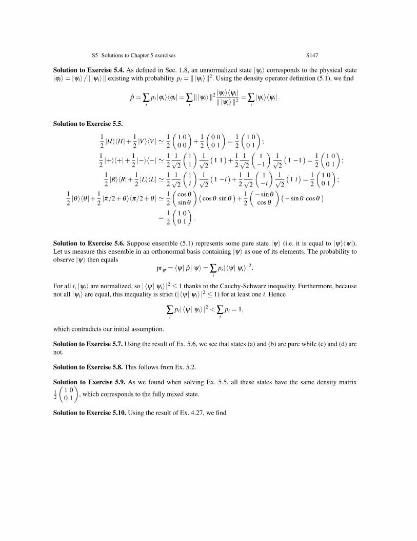
Solution to Exercise 5.5.
12|H〉〈H|+ 1
2|V 〉〈V | ' 1
2
(1 00 0
)+
12
(0 00 1
)=
12
(1 00 1
);
12|+〉〈+|+ 1
2|−〉〈−| ' 1
21√2
(11
)1√2
(1 1)+
12
1√2
(1−1
)1√2
(1 −1
)=
12
(1 00 1
);
12|R〉〈R|+ 1
2|L〉〈L| ' 1
21√2
(1i
)1√2
(1 −i
)+
12
1√2
(1−i
)1√2
(1 i)=
12
(1 00 1
);
12|θ〉〈θ |+ 1
2|π/2+θ〉〈π/2+θ | ' 1
2
(cosθ
sinθ
)(cosθ sinθ
)+
12
(−sinθ
cosθ
)(−sinθ cosθ
)=
12
(1 00 1
).
Solution to Exercise 5.6. Suppose ensemble (5.1) represents some pure state |ψ〉 (i.e. it is equal to |ψ〉〈ψ|).Let us measure this ensemble in an orthonormal basis containing |ψ〉 as one of its elements. The probability toobserve |ψ〉 then equals
prψ = 〈ψ| ρ| ψ〉= ∑i
pi| 〈ψ| ψi〉 |2.
For all i, |ψi〉 are normalized, so | 〈ψ| ψi〉 |2 ≤ 1 thanks to the Cauchy-Schwarz inequality. Furthermore, becausenot all |ψi〉 are equal, this inequality is strict (| 〈ψ| ψi〉 |2 ≤ 1) for at least one i. Hence
∑i
pi| 〈ψ| ψi〉 |2 < ∑i
pi = 1,
which contradicts our initial assumption.
Solution to Exercise 5.7. Using the result of Ex. 5.6, we see that states (a) and (b) are pure while (c) and (d) arenot.
Solution to Exercise 5.8. This follows from Ex. 5.2.
Solution to Exercise 5.9. As we found when solving Ex. 5.5, all these states have the same density matrix12
(1 00 1
), which corresponds to the fully mixed state.
Solution to Exercise 5.10. Using the result of Ex. 4.27, we find
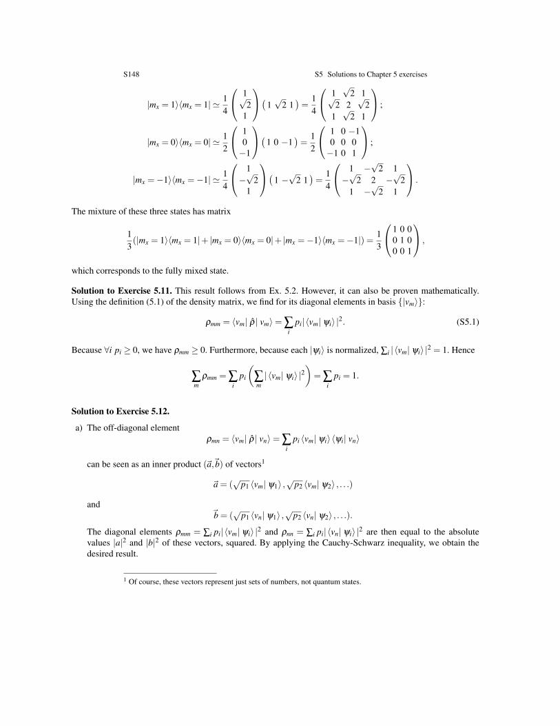
S148 S5 Solutions to Chapter 5 exercises
|mx = 1〉〈mx = 1| ' 14
1√2
1
(1√
2 1)=
14
1√
2 1√2 2
√2
1√
2 1
;
|mx = 0〉〈mx = 0| ' 12
10−1
(1 0 −1)=
12
1 0 −10 0 0−1 0 1
;
|mx =−1〉〈mx =−1| ' 14
1−√
21
(1 −√
2 1)=
14
1 −√
2 1−√
2 2 −√
21 −
√2 1
.
The mixture of these three states has matrix
13(|mx = 1〉〈mx = 1|+ |mx = 0〉〈mx = 0|+ |mx =−1〉〈mx =−1|) = 1
3
1 0 00 1 00 0 1
,
which corresponds to the fully mixed state.
Solution to Exercise 5.11. This result follows from Ex. 5.2. However, it can also be proven mathematically.Using the definition (5.1) of the density matrix, we find for its diagonal elements in basis |vm〉:
ρmm = 〈vm| ρ| vm〉= ∑i
pi| 〈vm| ψi〉 |2. (S5.1)
Because ∀i pi ≥ 0, we have ρmm ≥ 0. Furthermore, because each |ψi〉 is normalized, ∑i | 〈vm| ψi〉 |2 = 1. Hence
∑m
ρmm = ∑i
pi
(∑m| 〈vm| ψi〉 |2
)= ∑
ipi = 1.
Solution to Exercise 5.12.
a) The off-diagonal elementρmn = 〈vm| ρ| vn〉= ∑
ipi 〈vm| ψi〉〈ψi| vn〉
can be seen as an inner product (~a,~b) of vectors1
~a = (√
p1 〈vm| ψ1〉 ,√
p2 〈vm| ψ2〉 , . . .)
and~b = (
√p1 〈vn| ψ1〉 ,
√p2 〈vn| ψ2〉 , . . .).
The diagonal elements ρmm = ∑i pi| 〈vm| ψi〉 |2 and ρnn = ∑i pi| 〈vn| ψi〉 |2 are then equal to the absolutevalues |a|2 and |b|2 of these vectors, squared. By applying the Cauchy-Schwarz inequality, we obtain thedesired result.
1 Of course, these vectors represent just sets of numbers, not quantum states.
S5 Solutions to Chapter 5 exercises S149
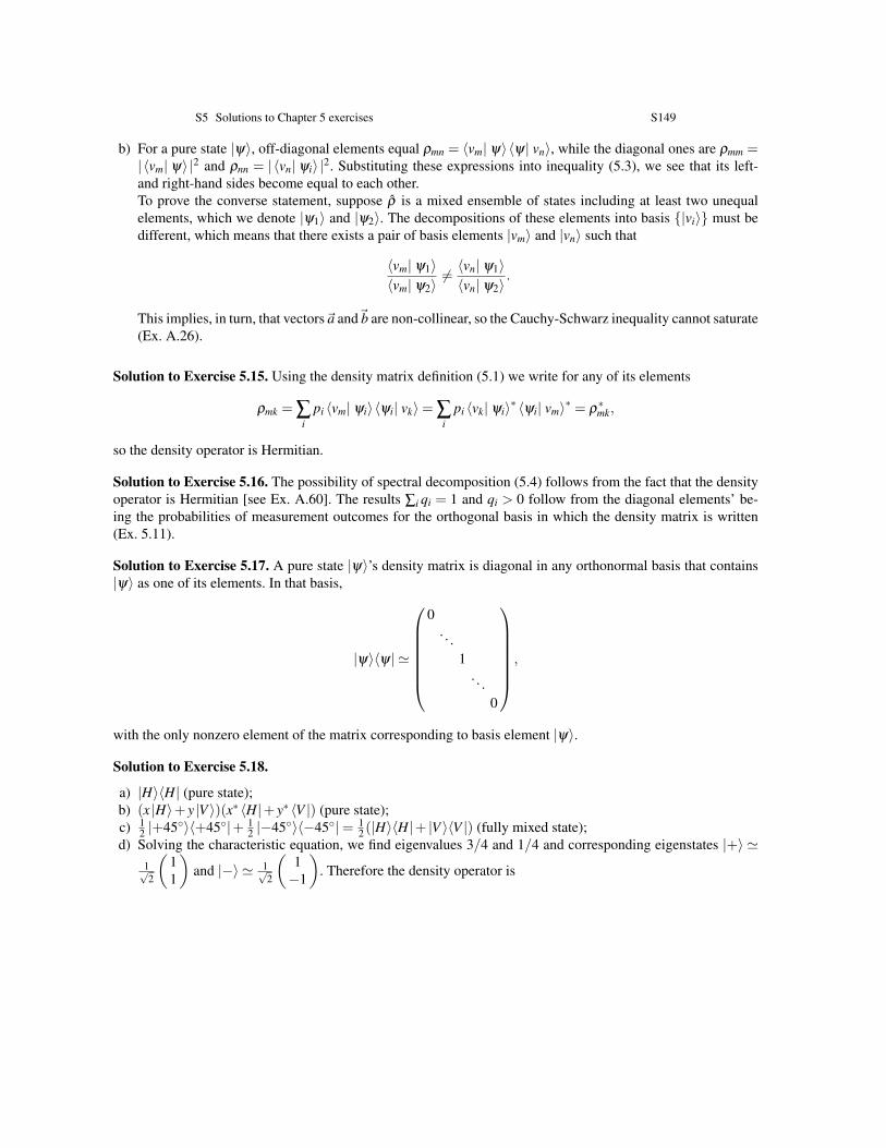
b) For a pure state |ψ〉, off-diagonal elements equal ρmn = 〈vm| ψ〉〈ψ| vn〉, while the diagonal ones are ρmm =| 〈vm| ψ〉 |2 and ρnn = | 〈vn| ψi〉 |2. Substituting these expressions into inequality (5.3), we see that its left-and right-hand sides become equal to each other.To prove the converse statement, suppose ρ is a mixed ensemble of states including at least two unequalelements, which we denote |ψ1〉 and |ψ2〉. The decompositions of these elements into basis |vi〉 must bedifferent, which means that there exists a pair of basis elements |vm〉 and |vn〉 such that
〈vm| ψ1〉〈vm| ψ2〉
6= 〈vn| ψ1〉〈vn| ψ2〉
.
This implies, in turn, that vectors~a and~b are non-collinear, so the Cauchy-Schwarz inequality cannot saturate(Ex. A.26).
Solution to Exercise 5.15. Using the density matrix definition (5.1) we write for any of its elements
ρmk = ∑i
pi 〈vm| ψi〉〈ψi| vk〉= ∑i
pi 〈vk| ψi〉∗ 〈ψi| vm〉∗ = ρ∗mk,
so the density operator is Hermitian.
Solution to Exercise 5.16. The possibility of spectral decomposition (5.4) follows from the fact that the densityoperator is Hermitian [see Ex. A.60]. The results ∑i qi = 1 and qi > 0 follow from the diagonal elements’ be-ing the probabilities of measurement outcomes for the orthogonal basis in which the density matrix is written(Ex. 5.11).
Solution to Exercise 5.17. A pure state |ψ〉’s density matrix is diagonal in any orthonormal basis that contains|ψ〉 as one of its elements. In that basis,
|ψ〉〈ψ| '
0
. . .1
. . .0
,
with the only nonzero element of the matrix corresponding to basis element |ψ〉.
Solution to Exercise 5.18.
a) |H〉〈H| (pure state);b) (x |H〉+ y |V 〉)(x∗ 〈H|+ y∗ 〈V |) (pure state);c) 1
2 |+45〉〈+45|+ 12 |−45〉〈−45|= 1
2 (|H〉〈H|+ |V 〉〈V |) (fully mixed state);d) Solving the characteristic equation, we find eigenvalues 3/4 and 1/4 and corresponding eigenstates |+〉 '
1√2
(11
)and |−〉 ' 1√
2
(1−1
). Therefore the density operator is
S150 S5 Solutions to Chapter 5 exercises
34|+〉〈+|+ 1
4|−〉〈−| '
(1/2 1/41/4 1/2
).
Solution to Exercise 5.19.
a) In the Fock basis:
(a |0〉+b |1〉)(a∗ 〈0|+b∗ 〈1|)'
aa∗ ab∗ 0 . . .ba∗ bb∗ 0 . . .0 0 0 . . ....
......
. . .
b) In the position basis, using wavefunctions ψ0(X) and ψ1(X) of the first two Fock states, given by Eqs. (3.106)
and (3.107), respectively, we find:
ρ(X ,X ′) = [aψ0(X)+bψ1(X)][a∗ψ∗0 (X′)+b∗ψ∗1 (X
′)]
= π−1/2e−(X2+X ′2)/2[a+bX
√2][a∗+b∗X ′
√2].
Solution to Exercise 5.20.
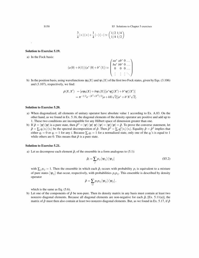
a) When diagonalized, all elements of unitary operator have absolute value 1 according to Ex. A.83. On theother hand, as we found in Ex. 5.16, the diagonal elements of the density operator are positive and add up to1. These two conditions are incompatible for any Hilbert space of dimension greater than one.
b) If ρ = |ψ〉〈ψ| is a pure state, then ρ2 = |ψ〉〈ψ| ψ〉〈ψ|= |ψ〉〈ψ|= ρ . To prove the converse statement, letρ = ∑i qi |vi〉〈vi| be the spectral decomposition of ρ . Then ρ2 = ∑i q2
i |vi〉〈vi|. Equality ρ = ρ2 implies thateither qi = 0 or qi = 1 for any i. Because ∑i qi = 1 for a normalized state, only one of the qi’s is equal to 1while others are 0. This means that ρ is a pure state.
Solution to Exercise 5.21.
a) Let us decompose each element ρi of the ensemble in a form analogous to (5.1):
ρi = ∑j
pi j∣∣ψi j
⟩⟨ψi j∣∣ (S5.2)
with ∑ j pi j = 1. Then the ensemble in which each ρi occurs with probability pi is equivalent to a mixtureof pure states
∣∣ψi j⟩
that occur, respectively, with probabilities pi pi j. This ensemble is described by densityoperator
ρ = ∑i j
pi pi j∣∣ψi j
⟩⟨ψi j∣∣ ,
which is the same as Eq. (5.6).b) Let one of the components of ρ be non-pure. Then its density matrix in any basis must contain at least two
nonzero diagonal elements. Because all diagonal elements are non-negative for each ρi [Ex. 5.11(a)], thematrix of ρ must then also contain at least two nonzero diagonal elements. But, as we found in Ex. 5.17, if ρ
S5 Solutions to Chapter 5 exercises S151
were pure, there would exist a basis in which its density matrix contains only one element. We have arrivedat a contradiction.
Solution to Exercise 5.22.
a) Using the representation of the density operator as a statistical ensemble (5.1), and using the Schrodingerequation (1.31) we have
˙ρ =ddt ∑
ipi |ψi〉〈ψi|
= ∑i
pi(|ψi〉〈ψi|+ |ψi〉〈ψi|)
= ∑i
pi(−ih
H |ψi〉〈ψi|+ |ψi〉〈ψi|ih
H)
= − ih(Hρ− ρH)
= − ih[H, ρ].
b) Using Eqs. (1.29) and (1.30), we find
ρ(t) = ∑i
pi |ψi(t)〉〈ψi(t)|
= ∑i
piU(t) |ψi(0)〉〈ψi(0)|U†(t)
= e−ih Ht
ρ(0)eih Ht ,
where U(t) = e−ih Ht is the evolution operator.
Solution to Exercise 5.23. If ρ(0) = ∑i pi |Ei〉〈Ei|, the evolution according to Eq. (5.8) is
ρ(t) = ∑i
pie−ih Ht |Ei〉〈Ei|e
ih Ht
= ∑i
pie−ih Eit |Ei〉〈Ei|e
ih EiHt
= ∑i
pi |Ei〉〈Ei|= ρ,
where we used the fact that each |Ei〉 is an eigenstate of H with eigenvalue Ei.
Solution to Exercise 5.24.
a) Since |ψ(0)〉= (|E1〉+ |E2〉)/√
2, and because |E1〉 and |E2〉 are eigenstates of the Hamiltonian, we have
|ψ(t)〉= e−ih Ht |ψ(0)〉= (e−
ih E1t |E1〉+ e−
ih E2t |E2〉)/
√2,
S152 S5 Solutions to Chapter 5 exercises
and thus
ρ(t) = |ψ(t)〉〈ψ(t)|= 12(|E1〉〈E1|+ e−
ih (E1−E2)t |E1〉〈E2|+ e−
ih (E2−E1)t |E2〉〈E1|+ |E2〉〈E2|).
b) Using Eq. (5.8),
ρ(t) = e−ih Ht
ρ(0)eih Ht
=12(e−
ih E1t |E1〉〈E1|e
ih E1t + e−
ih E2t |E2〉〈E2|e
ih E2t)
=12(|E1〉〈E1|+ |E2〉〈E2|)
= ρ(0).
Solution to Exercise 5.25.
a) The Hamiltonian is H =− 12 ΩLσx, where ΩL = γB is the Larmor frequency. The evolution operator for this
Hamiltonian has been found in Exercise 4.62(c). Specializing to θ0 = π/2, we have
e−ih Ht '
(cos(ΩLt/2) isin(ΩLt/2)isin(ΩLt/2) cos(ΩLt/2)
),
Hence
e−ih Ht |↑〉 '
(cos(ΩLt/2)isin(ΩLt/2)
);
e−ih Ht |↓〉 '
(isin(ΩLt/2)cos(ΩLt/2)
)Accordingly,
ρ(t) =34
e−ih Ht |↑〉Adjoint
(e−
ih Ht |↑〉
)+
14
e−ih Ht |↓〉Adjoint
(e−
ih Ht |↓〉
)'
14 +
12 cos2(ΩLt/2) − i
2 cos(ΩLt/2)sin(ΩLt/2)
i2 cos(ΩLt/2)sin(ΩLt/2) 3
4 −12 cos2(ΩLt/2)
.
b) The initial density matrix is
ρ(0) = 3/4 |↑〉〈↑|+1/4 |↓〉〈↓| '( 3
4 00 1
4
).
Applying the evolution operator directly to the density matrix according to Eq. (5.8), we obtain the sameresult:
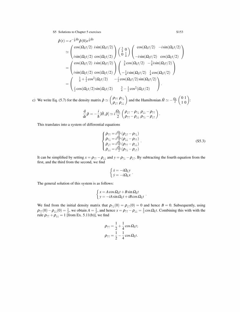
S5 Solutions to Chapter 5 exercises S153
ρ(t) = e−ih Ht
ρ(0)eih Ht
'
cos(ΩLt/2) isin(ΩLt/2)
isin(ΩLt/2) cos(ΩLt/2)
( 34 00 1
4
) cos(ΩLt/2) −isin(ΩLt/2)
−isin(ΩLt/2) cos(ΩLt/2)
=
cos(ΩLt/2) isin(ΩLt/2)
isin(ΩLt/2) cos(ΩLt/2)
34 cos(ΩLt/2) − 3
4 isin(ΩLt/2)
− 14 isin(ΩLt/2) 1
4 cos(ΩLt/2)
=
14 +
12 cos2(ΩLt/2) − i
2 cos(ΩLt/2)sin(ΩLt/2)
i2 cos(ΩLt/2)sin(ΩLt/2) 3
4 −12 cos2(ΩLt/2)
.
c) We write Eq. (5.7) for the density matrix ρ '(
ρ↑↑ ρ↑↓ρ↓↑ ρ↓↓
)and the Hamiltonian H '−ΩL
2
(0 11 0
):
ddt
ρ =− ih[H, ρ]' i
ΩL
2
(ρ↓↑−ρ↑↓ ρ↓↓−ρ↑↑ρ↑↑−ρ↓↓ ρ↑↓−ρ↓↑
).
This translates into a system of differential equationsρ↑↑ = i ΩL
2 (ρ↓↑−ρ↑↓)
ρ↑↓ = i ΩL2 (ρ↓↓−ρ↑↑)
ρ↓↑ = i ΩL2 (ρ↑↑−ρ↓↓)
ρ↓↓ = i ΩL2 (ρ↑↓−ρ↓↑)
. (S5.3)
It can be simplified by setting x = ρ↑↑−ρ↓↓ and y = ρ↑↓−ρ↓↑. By subtracting the fourth equation from thefirst, and the third from the second, we find
x =−iΩLyy =−iΩLx .
The general solution of this system is as follows:x = AcosΩLt +BsinΩLty =−iAsinΩLt + iBcosΩLt .
We find from the initial density matrix that ρ↑↓(0) = ρ↓↑(0) = 0 and hence B = 0. Subsequently, usingρ↑↑(0)−ρ↓↓(0) = 1
2 , we obtain A = 12 , and hence x = ρ↑↑−ρ↓↓ =
12 cosΩLt. Combining this with with the
rule ρ↑↑+ρ↓↓ = 1 [from Ex. 5.11(b)], we find
ρ↑↑ =12+
14
cosΩLt;
ρ↑↑ =12− 1
4cosΩLt.
S154 S5 Solutions to Chapter 5 exercises
Next, we look for the off-diagonal elements of ρ(t). Because ρ↓↑ = i ΩL2 (ρ↓↓−ρ↑↑) [from Eq. (S5.3)], we
findρ↓↑ =
i4
sinΩLt +C
with C = 0 from the initial density matrix. Finally,
ρ↑↓ = ρ∗↓↑ =−
i4
sinΩLt.
To summarize, the density matrix is
ρ(t)'( 1
2 +14 cosΩLt − i
4 sinΩLti4 sinΩLt 1
2 −14 cosΩLt
). (S5.4)
Using the trigonometric identities cos(ΩLt/2)sin(ΩLt/2) = 12 sinΩLt and cos2(ΩLt/2) = 1
2 +12 cosΩLt, we
find our result to be identical to that of parts (a) and (b).
Solution to Exercise 5.26. Let |vi〉 and ∣∣w j⟩ be two different bases in V. Then the trace of the matrix in
basis |vi〉 isTr(A) = ∑
iAii = ∑
i〈vi| A |vi〉 (S5.5)
Inserting identity operators, we see
Tr(A) = ∑i〈vi| 1A1 |vi〉
= ∑i, j,k
⟨vi∣∣ w j
⟩⟨w j∣∣ A |wk〉〈wk| vi〉
= ∑i, j,k〈wk| vi〉
⟨vi∣∣ w j
⟩⟨w j∣∣ A |wk〉
= ∑j,k〈wk|
(∑
i|vi〉〈vi|
)∣∣w j⟩⟨
w j∣∣ A |wk〉
= ∑j,k〈wk| 1
∣∣w j⟩⟨
w j∣∣ A |wk〉
= ∑j,k
δ jk⟨w j∣∣ A |wk〉
= ∑j
⟨w j∣∣ A ∣∣w j
⟩,
hence the trace is basis-independent.
Solution to Exercise 5.27. This statement is the same as that of Ex. 5.11(b).
Solution to Exercise 5.29.
S5 Solutions to Chapter 5 exercises S155
a) This follows from Ex. 5.28.b) This follows from part (a) if we denote A1 . . . Ak−1 = A and Ak = B.
Solution to Exercise 5.30. For Pauli matrices, we have
σxσyσz =
(i 00 i
)and
σyσxσz =
(−i 00 −i
).
In the first case the trace equals 2i, in the second case −2i.
Solution to Exercise 5.31. Using Ex. 5.28, we have
Tr(A |ϕ〉〈ψ|) = ∑mn
⟨vn∣∣ A∣∣ vm
⟩〈vm|(|ϕ〉〈ψ|) |vn〉
= ∑mn〈ψ| vn〉
⟨vn∣∣ A∣∣ vm
⟩〈vm| ϕ〉
= 〈ψ|(
∑n|vn〉〈vn|
)A(
∑n|vn〉〈vn|
)|ϕ〉
=⟨ψ∣∣ A∣∣ ϕ⟩.
Solution to Exercise 5.32. If ρ = |ψ〉〈ψ| is a pure state, then ρ2 = ρ , so Tr(ρ2) = 1. If the state is non-pure,the diagonalized form of its density matrix ρ ' diag(ρ11, . . . ,ρNN) has at least two nonzero elements. BecauseTrρ = 1, we have ρii < 1 for any i, and hence ρ2
ii < ρii. Therefore
Tr(ρ2) = ∑i
ρ2ii < ∑
iρii = Trρ = 1.
To prove the other inequality, let us consider the scalar product of vectors ~a = (ρ11, . . . ,ρNN) and ~b =(1, . . . ,1). According to the Cauchy-Schwarz inequality,
(~a ·~b)2 ≤ (~a ·~a)× (~b ·~b),
or (∑
iρii
)2
≤∑i
ρ2ii×N.
The left-hand side of the above inequality is (Trρ)2 = 1. Therefore Tr(ρ2) = ∑i ρ2ii ≥ 1/N, with the inequality
saturating for~a ∝~b, i.e. for the fully mixed state ρ ' diag(1/N, . . . ,1/N).
Solution to Exercise 5.33.
S156 S5 Solutions to Chapter 5 exercises
a) Let us once again recall that the density matrix is an expression (5.1) for the statistical ensemble of purestates. As we found in Sec. 1.9.1, upon detection of basis element |vm〉 in a measurement, each componentof the ensemble transforms according to |ψi〉 → Πm |ψi〉. The whole ensemble will therefore transform asfollows:
ρ = ∑i
pi |ψi〉〈ψi| → ∑i
piΠm |ψi〉〈ψi|Πm = ΠmρΠm. (S5.6)
Here we used the Hermitian nature of the projection operator.b) For each component |ψi〉 of the ensemble, the probability of detecting |vm〉 is prm|i = | 〈vm| ψi〉 |2, so the
probability of detecting |vm〉 for the full density matrix is (see Ex. B.6)
prm = ∑i
piprm|i
= ∑i
pi| 〈vm| ψi〉 |2
= ∑i
pi 〈vm| ψi〉〈ψi| vm〉
Ex. 5.31= Tr
[(∑
ipi |ψi〉〈ψi|
)(|vm〉〈vm|)
]= Tr[ρΠm]
Ex. 5.29(a)= Tr[Πmρ]
Solution to Exercise 5.34. The projector onto |+45〉 is
Π+ = |+〉〈+|= 12
(1 11 1
).
Accordingly, using the density matrices from Ex. 5.1, we find
a)
Tr[Π+ρ] =12
Tr(
1 01 0
)=
12,
consistent with | 〈+| H〉 |2 = 12 ;
b)
Tr[Π+ρ] =12
Tr(|ψH |2 +ψ∗HψV ψHψ∗V + |ψV |2|ψH |2 +ψ∗HψV ψHψ∗V + |ψV |2
)=
12(|ψH |2 +ψHψ
∗V +ψ
∗HψV + |ψV |2) =
12|ψH +ψV |2,
consistent with | 〈+|(ψH |H〉+ψV |V 〉)|2 = | 1√2(〈H|+ 〈V |)(ψH |H〉+ψV |V 〉)|2 = 1
2 |ψH +ψV |2;c)
Tr[Π+ρ] =14
Tr(
1 11 1
)=
12,
consistent with p1| 〈+|+〉 |2 + p2| 〈+| −〉|2 = 12 +0 = 1
2 ;d)
S5 Solutions to Chapter 5 exercises S157
Tr[Π+ρ] = Tr
38
38
38
38
=34,
consistent with p1| 〈+|+〉 |2 + p2| 〈+| H〉 |2 + p3| 〈+|V 〉 |2 = 12 +
18 +
18 = 3
4 .
Solution to Exercise 5.35. We know from Ex. 5.33 that the unnormalized state after the measurement, if result|vm〉 is obtained, is given by ΠmρΠm = 〈vm| ρ| vm〉 |vm〉〈vm|. If the measurement result is unknown, we have tosum this expression over all m’s according to Ex. 5.4:
∑m〈vm| ρ| vm〉 |vm〉〈vm| . (S5.7)
The matrix of this operator in basis |vm〉 is given by expression (5.15).
Solution to Exercise 5.36. Writing the definition (1.12) of observable operator in the form V = ∑i vi |vi〉〈vi| =∑i viΠi, we have
Tr(V ρ) = ∑i
viTr(Πiρ)(5.13)= ∑
ivipri
(B.1)= 〈V 〉 ,
where pri = Tr(Πiρ) is the probability of projecting ρ onto eigenstate |vi〉 of V .
Solution to Exercise 5.37.
a) We write ρAB = ∑i pi |Ψi〉 in accordance with the density operator definition (5.1), with |Ψi〉 being bipartitestates (pure, but not necessarily separable). As we found in Chapter 2 [see Eq. (2.22)], Alice’s measurementof state |Ψi〉, which results in observation of element |vm〉 of her measurement basis, transforms |Ψi〉 intounnormalized state ΠA,m |Ψi〉. Accordingly, the full density matrix becomes
ρAB,m →∑i
piΠA,m |Ψi〉〈Ψi|ΠA,m
= ΠA,m
(∑
ipi |Ψi〉〈Ψi|
)ΠA,m
= ΠA,mρABΠA,m
= |vm〉〈vm|⊗ 〈vm| ρAB| vm〉 . (S5.8)
Bob’s portion of this bipartite state is ρB,m = 〈vm| ρAB| vm〉.b) If Alice’s measurement result is unknown, Bob has a probabilistic ensemble of ρB,m for different m’s, so its
density operator is the sum of unnormalized individual density matrices as per Ex. 5.4:
ρB = ∑m〈vm| ρAB| vm〉= TrA(ρAB).
Solution to Exercise 5.38.
a) The proof is analogous to that in Ex. 5.26.
S158 S5 Solutions to Chapter 5 exercises
b) Let us calculate the trace of ρAB in basis |vm〉⊗|wn〉, where |vn〉 |wn〉 are orthonormal bases in Alice’sand Bob’s spaces, respectively. We find
TrρAB = ∑mn(〈vm|⊗ 〈wn|)(ρAB)(|vm〉⊗ |wn〉)
= ∑n〈wn|
(∑m〈vm| ρAB |vm〉
)|wn〉
= Tr(TrAρAB).
If the left-hand side of the above equation is 1, so must be its right-hand side.
Solution to Exercise 5.39. For Bell state |Φ+〉,
ρB = TrA∣∣Φ+
⟩⟨Φ
+∣∣
=12〈H|A (|HH〉+ |VV 〉)(〈HH|+ 〈VV |) |H〉A +
12〈V |A (|HH〉+ |VV 〉)(〈HH|+ 〈VV |) |V 〉A
=12|H〉B 〈H|B +
12|V 〉B 〈V |B ,
i.e. the fully mixed state. For the three other Bell states, the calculation is analogous and the result is the same.
Solution to Exercise 5.40.
a) Similarly to the previous exercise,
ρB = TrA |Ψ〉〈Ψ |
=15〈H|A (|HH〉+2 |VV 〉)(〈HH|+2〈VV |) |H〉A +
15〈V |A (|HH〉+2 |VV 〉)(〈HH|+2〈VV |) |V 〉A
=15|H〉B 〈H|B +
45|V 〉B 〈V |B
'(
1/5 00 4/5
)This is consistent with the verbal description of Bob’s photon found in the solution to Ex. 2.43: “either|H〉 with probability 1/5 or |V 〉 with probability 4/5”. It is also consistent with the alternative description:“either
√1/5 |H〉+
√4/5 |V 〉 or
√1/5 |H〉−
√4/5 |V 〉 with probabilities 1/2” because this ensemble has
the density matrix12
(1/5 2/52/5 4/5
)+
12
(1/5 −2/5−2/5 4/5
)=
(1/5 00 4/5
).
b) Similarly to the previous exercise,
S5 Solutions to Chapter 5 exercises S159
ρB = TrA |Ψ〉〈Ψ |
=13〈H|A (|HH〉+ |HV 〉+ |VV 〉)(〈HH|+ 〈HV |+ 〈VV |) |H〉A
+13〈V |A (|HH〉+ |HV 〉+ |VV 〉)(〈HH|+ 〈HV |+ 〈VV |) |V 〉A
=13(|H〉B + |V 〉B)(〈H|B + 〈V |B)+
13|V 〉B 〈V |B
'(
1/3 1/31/3 2/3
).
The verbal descriptions of Bob’s photon found in the solution to Ex. 2.43 are “either |+〉with probability 2/3or |V 〉 with probability 1/3” and “either
√1/5 |H〉+
√4/5 |V 〉 with probability 5/6 or |H〉 with probability
1/6”. Indeed, these ensembles corresponds to the density matrices
23
(1/2 1/21/2 1/2
)+
13
(0 00 1
)=
(1/3 1/31/3 2/3
)and
56
(1/5 2/52/5 4/5
)+
16
(1 00 0
)=
(1/3 1/31/3 2/3
),
i.e. the same as what we found by taking the partial trace.
Solution to Exercise 5.41.
a) If ρAB = |φ〉〈φ |⊗ |ψ〉〈ψ| (where states |φ〉 and |ψ〉 live, respectively, in Alice’s and Bob’s Hilbert spaces),then for any element |vm〉 of Alice’s basis we have 〈vm| ρAB |vm〉= | 〈vm| φ〉 |2 |ψ〉〈ψ| and hence
TrA(ρAB) =
(∑m| 〈vm| φ〉 |2
)|ψ〉〈ψ| ,
which is a separable state. The argument for tracing over Bob’s space is analogous.b) Let us first assume the entangled bipartite state to be pure: ρAB = |Ψ〉〈Ψ |. We can decompose this state as
we did in Sec. 2.2.2: |Ψ〉= ∑i1Ni|vi〉⊗|bi〉, where |vi〉 is an orthonormal basis in Alice’s space and |bi〉
is a set of normalized vectors in Bob’s space. Tracing this over Alice’s Hilbert space, we have
ρB = TrA |Ψ〉〈Ψ |= ∑i
1N2
i|bi〉〈bi| .
If |Ψ〉 is entangled, at least two of the |bi〉’s are different, so ρB is mixed.For a non-pure ρAB = ∑i pi |Ψi〉〈Ψi|, we have TrA(ρAB) = ∑i piTrA |Ψi〉〈Ψi|. This is a statistical mixture ofmixed states, which, as we have shown in Ex. 5.21, cannot be pure.
Solution to Exercise 5.42. Suppose the system is in initial state ρS = ∑i j ρi j |vi〉⟨v j∣∣. The von Neumann mea-
surement brings about the state
S160 S5 Solutions to Chapter 5 exercises
ρSA = ∑i j
ρi j(|vi〉⟨v j∣∣)system⊗ (|wi〉
⟨w j∣∣)apparatus
Tracing over the apparatus in basis |wk〉], we find
ρ′S = ∑
i jkρi j(|vi〉
⟨v j∣∣)system 〈wk| wi〉
⟨w j∣∣ wk
⟩= ∑
i jkρi j(|vi〉
⟨v j∣∣)systemδikδ jk
= ∑k
ρkk(|vk〉〈vk|)system,
which corresponds to a diagonal density matrix in basis |vk〉].
Solution to Exercise 5.43. For ρ = ∑i pi |ψi〉〈ψi|, the expectation value of Pauli observable σx is
〈σx〉(5.16)= Tr(ρσx) = ∑
ipiTr(|ψi〉〈ψi| σx)
(5.11)= ∑
ipi 〈ψi| σx| ψi〉
Ex. 4.48(c)= ∑
ipiRxi.
The arguments for the y and z components of the Bloch vector are analogous.
Solution to Exercise 5.44. The density matrix found in Ex. 5.25 is
ρ(t)'( 1
2 +14 cosΩLt − i
4 sinΩLti4 sinΩLt 1
2 −14 cosΩLt
). (S5.9)
The components of the Bloch vector associated with this state are
Rx(t) = Tr(ρσx) = 0;
Ry(t) = Tr(ρσy) =12
sinΩLt;
Ry(t) = Tr(ρσz) =12
cosΩLt;
The corresponding trajectory of the Bloch vector is a circle of radius 12 in the y-z plane, which corresponds to the
precession around the x axis.
Solution to Exercise 5.45.
a) An ensemble average ~Rρ = ∑i pi~Ri of unequal geometric vectors of length 1 has length less than 1. To provethis rigorously, we find for the length of the Bloch vector

S5 Solutions to Chapter 5 exercises S161
|Rρ |2 = ~Rρ ·~Rρ
= ∑i j
pi p j~Ri ·~R j
< ∑i j
pi p j|Ri||R j|
=
(∑
ipi|Ri|
)2
=
(∑
ipi
)2
= 1.
We have used the Cauchy-Schwarz inequality. It is strict because at least two of the ~Ri’s correspond tounequal states and are hence non-collinear. We also used the fact that |Ri|= 1 for a pure state.
b) The fully mixed state is an equal mixture of states |↑〉 and |↓〉. The Bloch vector of state |↑〉 points along thepositive z axis while that of state |↓〉 along the negative z axis. Both these vectors have length 1, so their sumis zero.
Solution to Exercise 5.46. Given spectral decomposition
ρ = p |v1〉〈v1|+(1− p) |v2〉〈v2| , (S5.10)
we findρ
2 = p2 |v1〉〈v1|+(1− p)2 |v2〉〈v2|
and henceTrρ2 = p2 +(1− p)2 = 2p2−2p+1. (S5.11)
To find the length of the Bloch vector corresponding to state (S5.10), we notice that the Bloch vectors of orthog-onal pure states |v1〉 and |v2〉 are opposite and have length 1. The geometric sum of these vectors with weights pand 1− p gives a vector of length
|Rρ |= |p− (1− p)|= |2p−1|. (S5.12)
Combining Eqs. (S5.11) and (S5.12), we obtain Eq. (5.21).
Solution to Exercise 5.47. Let us consider an arbitrary vector ~R of length 0 < |R| ≤ 1 and find normalized stateρ such that ~R is its Bloch vector. This state has spectral decomposition
ρ = p |v1〉〈v1|+(1− p) |v2〉〈v2| (S5.13)
into orthogonal pure states |v1〉 and |v2〉. Let ~R1 and ~R2 be the Bloch vectors of these states. Then
~R = p~R1 +(1− p)~R2. (S5.14)
Vectors ~R1 and ~R2 have length 1 and are opposite in direction. Therefore, in order to satisfy Eq. (S5.14), thesevectors must be collinear with ~R, and hence Eq. (S5.14) has a unique (up to a transposition of ~R1 and ~R2) solution;
S162 S5 Solutions to Chapter 5 exercises
~R1 = ~R/|R|, ~R2 =−~R1 and p = (1+ |R|)/2. These vectors uniquely define the corresponding states |v1〉 and |v2〉,which, in turn, uniquely define the density operator (S5.13) whose Bloch vector is ~R.
Solution to Exercise 5.48.
a) Since the components of Bloch vector are the mean values of the corresponding Pauli operators,
R j =⟨σ j⟩ (5.16)
= Tr(ρσ j),
the time derivative of the Bloch vector in the Schrodinger picture is
ddt
R j = Tr(
dρ
dtσ j
)(5.30)= − i
hTr[[H, ρ]σ j
](S5.15)
We now use the chain rule for the trace [Ex. 5.29(b)] to write
− ih
Tr[[H, ρ]σ j
]=− i
hTr[Hρσ j− ρHσ j
]]
=− ih
Tr[ρσ jH− ρHσ j
]=
ih
Tr[ρ[H, σ j]
]=
ih
⟨[H, σ j]
⟩.
b) Now specializing to the magnetic field Hamiltonian (4.76), which we rewrite as H =− γ
h 2σkBk, we find
ddt
R j =ih
⟨[H, σ j]
⟩=− iγ
2⟨[σk, σ j]
⟩Bk
(A.47)= − iγ
2⟨2iεk jmσm
⟩Bk
= γεk jm 〈σm〉Bk
= γε jmkRmBk
= γ[~R×~B] j,
where we have used the Levi-Civita symbol for the vector product.
Solution to Exercise 5.49. Suppose at a given time t the spin state is given by
ρ(t) =(
ρ↑↑(t) ρ↑↓(t)ρ↓↑(t) ρ↓↓(t)
).
After a short interval ∆ t, it will decohere, i.e. become
S5 Solutions to Chapter 5 exercises S163
ρdec(t) =(
ρ↑↑(t) 00 ρ↓↓(t)
)with probability ∆ t/T2, and remain the same with probability 1−∆ t/T2. Accordingly, the density matrix atmoment t +∆ t is
ρ(t +∆ t) = (1−∆ t/T2)ρ(t)+(∆ t/T2)ρdec(t)
=
(ρ↑↑(t) (1−∆ t/T2)ρ↑↓(t)
(1−∆ t/T2)ρ↓↑(t) ρ↓↓(t)
).
The change of the off-diagonal elements during time ∆ t can hence be written as
∆ρi j(t) =−(∆ t/T2)ρi j(t).
Dividing both sides of this equation by ∆ t, we obtain Eq. (5.23) in the limit ∆ t→ 0.
Solution to Exercise 5.50. If the dc field has been turned on for a long enough time for the spins to thermalize,the ratio of their probabilities will be determined by Boltzmann’s law:
pr↓pr↑
= exp(−γ hB0
kT
)(4.70)= exp
(− gehB0
2MpkT
)≈ exp
(−1.1×10⁻⁵
)≈ 1−1.1×10⁻⁵,
where the mass and Lande factor of the proton are found in Table 4.3. Because this ratio is close to unity, bothprobabilities are close to 0.5 so pr↓−pr↑ ≈−0.55×10⁻⁵.
Solution to Exercise 5.51. Solving the system of equationsρ↓↓,0/ρ↑↑,0 = e−
γ hB0kT
ρ↓↓,0 +ρ↑↑,0 = 1,
we find ρ↑↑,0 =
12 +
12 e−
γ hB0kT
ρ↓↓,0 =12 −
12 e−
γ hB0kT
.
This corresponds to a Bloch vector of length e−γ hB0
kT pointing straight up.
Solution to Exercise 5.53. In the presence of relaxation, Eq. (S5.15) for the Bloch vector evolution obtains anadditional term, which unites the decoherence and thermalization terms of Eq. (5.30):
ddt~R =− i
hTr[[H, ρ]~σ
]+Tr
[(dρ
dt
)relax
~σ
]. (S5.16)
The first term in the above equation has already been shown in the solution to Ex. 5.48 to read to the first termin each of the Eqs. 5.31. For the relaxation term, we bring together Eqs. (5.23) and (5.29) to write(
dρi j
dt
)relax
=
−[ρii(t)−ρii,0]/T1, i = j−ρi j(t)/T2, i 6= j , (S5.17)
S164 S5 Solutions to Chapter 5 exercises
or, explicitly, (dρ
dt
)relax'(−[ρ↑↑(t)−ρ↑↑,0]/T1 −ρ↑↓(t)/T2−ρ↓↑(t)/T2 −[ρ↓↓(t)−ρ↓↓,0]/T1
). (S5.18)
From this result, we can calculate the second term of Eq. (S5.15) for each Pauli operator:
Tr[(
dρ
dt
)relax
σx
]=−[ρ↑↓(t)+ρ↓↑(t)]/T2;
Tr[(
dρ
dt
)relax
σx
]=−i[ρ↑↓(t)−ρ↓↑(t)]/T2;
Tr[(
dρ
dt
)relax
σx
]=−[ρ↑↑(t)−ρ↓↓(t)]/T1 +[ρ↑↑,0(t)−ρ↓↓,0(t)]/T1.
Observing that the components of the Bloch vector are related to the density matrix elements according to
Rx = Tr[ρσx] = ρ↑↓(t)+ρ↓↑(t);Ry = Tr[ρσx] = iρ↑↓(t)− iρ↓↑(t);Rz = Tr[ρσx] = ρ↑↑(t)−ρ↓↓(t),
we obtain the second term in Eqs. (5.31).
Solution to Exercise 5.54. In the absence of the rf field, the fictitious magnetic field (4.86) has only the zcomponent which is determined by the detuning: Bz =−∆/γ . Substituting this into differential equations (5.31),we obtain
Rx(t) = −∆Ry−Rx(t)/T2;Ry(t) = ∆Rx−Ry(t)/T2; (S5.19)Rz(t) = −[Rz(t)−R0]/T1,
On can verify by direct substitution that Eqs. (5.32) solve these equations.
Solution to Exercise 5.56. Polar coordinates (θ ,0) of the initial Bloch vector correspond to Cartesian coordi-nates ~R(0) = (sinθ ,0,cosθ). We take the derivative of the Bloch vector length according to Eqs. (5.31):
ddt|~R(t)|2
∣∣∣∣t=0
= 2(RxRx +RyRy +RzRz
)∣∣t=0
=−2sin2
θ
T2+2cosθ
1− cosθ
T1
=−2sin2
θ
T2+2
cosθ
T1−2
cos2 θ
T1.
Approximating sin2θ ≈ θ 2, cosθ ≈ 1−θ 2/2, cos2 θ ≈ 1−θ 2 for small θ , we obtain
ddt|~R(t)|2
∣∣∣∣t=0≈−2
θ 2
T2− θ 2
T1+2
θ 2
T1=−2
θ 2
T2+
θ 2
T1.
S5 Solutions to Chapter 5 exercises S165
This derivative cannot be positive because the length of the Bloch vector is already at the maximum possiblevalue of 1 at t = 0. This means that −2/T2 +1/T1 ≤ 0 or T1 ≥ T2/2.
Solution to Exercise 5.57. Let us first track the evolution of the Bloch vector associated with a specific detuning∆ akin to what we did when solving Ex. 4.74. Applying a π/2 pulse to the spin-up state will transform it intothe state with the spin pointing along the y axis, so ~R(0) = (0,1,0). After the rf field has been turned off, theevolution is governed by Eqs. (5.32):
~R(t) =(−sin∆ te−t/T2 ,cos∆ te−t/T2 ,1− e−t/T1
).
The π pulse at t = t0 rotates the spin by 180 around the x axis, resulting in
~R(t0) = (−sin∆ t0e−t0/T2 ,−cos∆ t0e−t0/T2 ,−1+ e−t0/T1).
Subsequent evolution yields
~R(t) =[(−sin∆ t0 cos∆(t− t0)+ cos∆ t0 sin∆(t− t0))e−t/T2 ,
(−sin∆ t0 sin∆(t− t0)− cos∆ t0 cos∆(t− t0))e−t0/T2 ,
1+[−2+ e−t0/T1 ]e−(t−t0)/T1]
= (sin∆(t−2t0)e−t/T2 ,−cos∆(t−2t0)e−t/T2 ,1−2e−(t−t0)/T1 + e−t/T1).
Now integrating the y component of that vector over all detunings, we find, by analogy with the previous exercise,
〈µx〉= 0;⟨µy⟩=− hγ
2e−
[∆0(t−2t0)]2
4 e−t/T2 ;
〈µz〉= 1−2e−(t−t0)/T1 + e−t/T1 .
Solution to Exercise 5.58. The thermal state is characterized by Bloch vector ~R0(5.26)= (0,0,R0z), where R0z =
e−γ hB0
kT . The initial π pulse will flip this vector so that ~R(0) = (0,0,−R0z). The subsequent evolution accordingto Eqs. (5.32) is as follows:
~R(t) = (0,0,R0 +[Rz(0)−R0]e−t/T1) = (0,0,Rz0(1−2e−t/T1).
We see that ~R(t) = 0 when e−t/T1 = 1/2 or t = T1 ln2.
Solution to Exercise 5.59. We have µHH = 3/4, µHV = 1/4,µV H = 1/3, µVV = 2/3. Accordingly,
Solution to Exercise 5.60. ∑ j µi j is the sum of the probabilities for all possible mappings of the ith output of theclassic measurement device onto the outputs of the scrambler. Because one and only one of the mappings occurswith certainty, this sum is equal to one.
S166 S5 Solutions to Chapter 5 exercises
Solution to Exercise 5.61. Suppose n photons are incident on the detector. Each of these photons will generatean avalanche with probability η . The “no click” state will occur if none of the photons generate an avalanche,which happens with probability (1−η)n. Hence µn,no click = (1−η)n. Hence µn,no click +µn,click = 1 (Ex. 5.60),we have µn,click = 1− (1−η)n.
Solution to Exercise 5.62.
a) Using the result of Ex. 5.59 and summing over all possible output states of the quantum mesaurement deviceaccording to Eq. (5.34), we find
FH =µHH |H〉〈H|+µV H |V 〉〈V |=(
3/4 00 1/3
);
FV =µHV |H〉〈H|+µVV |V 〉〈V |=(
1/4 00 2/3
).
b) Similarly, using the result of Ex. 5.61, we obtain Eqs. (5.35).
Solution to Exercise 5.63.M
∑j=1
Fj =M
∑j=1
N
∑i=1
Πiµi jEx. 5.60=
N
∑i=1
Πi = 1.
Solution to Exercise 5.64.
a) Using the result of Ex. B.6, we find
pr j = ∑i
µi jpri(5.13)= ∑
iµi jTr(Πiρ) = Tr(∑
iµi jΠiρ) = Tr(Fjρ),
b) Similarly,
pr j = ∑i
µi jρB,i(5.18)= ∑
iµi jTrA(ΠiρAB) = TrA(FjρAB),
where ρB,i is Bob’s state in the event Alice detected |vi〉.
Solution to Exercise 5.65.Method 1: using the pure state and projective measurement formalism
a) We use the model of Fig. 5.2, i.e. assume that Alice’s detector consists of a pure quantum polarizationmeasurement device followed by a scrambler. There are four possibilities that define Bob’s ensemble.• The initial state is |Ψ1〉 and Alice’s quantum polarization measurement detects |H〉. In this case, the
unnormalized state of Bob’s photon is 〈H|Ψ1〉= (|H〉+ |V 〉)/√
6. The probability that Alice’s scramblerwill map her result onto output state H is 3/4.
• The initial state is |Ψ1〉 and Alice’s quantum polarization measurement detects |V 〉. In this case, theunnormalized state of Bob’s photon is 〈H|Ψ1〉 = 2 |V 〉/
√6. The probability that Alice’s scrambler will
map her result onto output state H is 1/3.
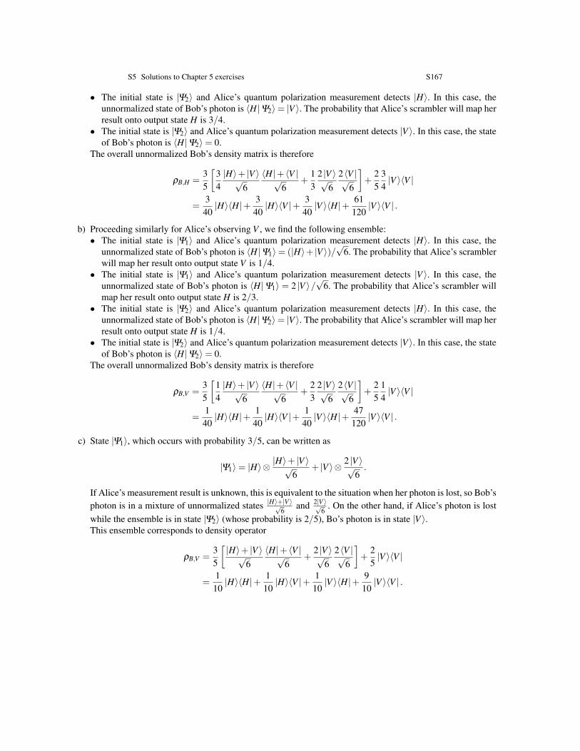
S5 Solutions to Chapter 5 exercises S167
• The initial state is |Ψ2〉 and Alice’s quantum polarization measurement detects |H〉. In this case, theunnormalized state of Bob’s photon is 〈H|Ψ2〉= |V 〉. The probability that Alice’s scrambler will map herresult onto output state H is 3/4.
• The initial state is |Ψ2〉 and Alice’s quantum polarization measurement detects |V 〉. In this case, the stateof Bob’s photon is 〈H|Ψ2〉= 0.
The overall unnormalized Bob’s density matrix is therefore
ρB,H =35
[34|H〉+ |V 〉√
6〈H|+ 〈V |√
6+
13
2 |V 〉√6
2〈V |√6
]+
25
34|V 〉〈V |
=340|H〉〈H|+ 3
40|H〉〈V |+ 3
40|V 〉〈H|+ 61
120|V 〉〈V | .
b) Proceeding similarly for Alice’s observing V , we find the following ensemble:• The initial state is |Ψ1〉 and Alice’s quantum polarization measurement detects |H〉. In this case, the
unnormalized state of Bob’s photon is 〈H|Ψ1〉= (|H〉+ |V 〉)/√
6. The probability that Alice’s scramblerwill map her result onto output state V is 1/4.
• The initial state is |Ψ1〉 and Alice’s quantum polarization measurement detects |V 〉. In this case, theunnormalized state of Bob’s photon is 〈H|Ψ1〉 = 2 |V 〉/
√6. The probability that Alice’s scrambler will
map her result onto output state H is 2/3.• The initial state is |Ψ2〉 and Alice’s quantum polarization measurement detects |H〉. In this case, the
unnormalized state of Bob’s photon is 〈H|Ψ2〉= |V 〉. The probability that Alice’s scrambler will map herresult onto output state H is 1/4.
• The initial state is |Ψ2〉 and Alice’s quantum polarization measurement detects |V 〉. In this case, the stateof Bob’s photon is 〈H|Ψ2〉= 0.
The overall unnormalized Bob’s density matrix is therefore
ρB,V =35
[14|H〉+ |V 〉√
6〈H|+ 〈V |√
6+
23
2 |V 〉√6
2〈V |√6
]+
25
14|V 〉〈V |
=1
40|H〉〈H|+ 1
40|H〉〈V |+ 1
40|V 〉〈H|+ 47
120|V 〉〈V | .
c) State |Ψ1〉, which occurs with probability 3/5, can be written as
|Ψ1〉= |H〉⊗|H〉+ |V 〉√
6+ |V 〉⊗ 2 |V 〉√
6.
If Alice’s measurement result is unknown, this is equivalent to the situation when her photon is lost, so Bob’sphoton is in a mixture of unnormalized states |H〉+|V 〉√
6and 2|V 〉√
6. On the other hand, if Alice’s photon is lost
while the ensemble is in state |Ψ2〉 (whose probability is 2/5), Bo’s photon is in state |V 〉.This ensemble corresponds to density operator
ρB,V =35
[|H〉+ |V 〉√
6〈H|+ 〈V |√
6+
2 |V 〉√6
2〈V |√6
]+
25|V 〉〈V |
=1
10|H〉〈H|+ 1
10|H〉〈V |+ 1
10|V 〉〈H|+ 9
10|V 〉〈V | .
S168 S5 Solutions to Chapter 5 exercises
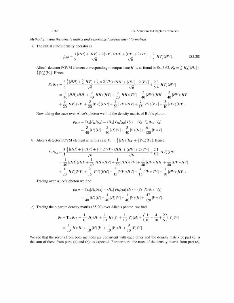
Method 2: using the density matrix and generalized measurement formalism
a) The initial state’s density operator is
ρAB =35|HH〉+ |HV 〉+2 |VV 〉√
6〈HH|+ 〈HV |+2〈VV |√
6+
25|HV 〉〈HV | . (S5.20)
Alice’s detector POVM element corresponding to output state H is, as found in Ex. 5.62, FH = 34 |HA〉〈HA|+
13 |VA〉〈VA|. Hence
FH ρAB =35
34 |HH〉+ 3
4 |HV 〉+ 13 ×2 |VV 〉
√6
〈HH|+ 〈HV |+2〈VV |√6
+25
34|HV 〉〈HV |
=3
40|HH〉〈HH|+ 3
40|HH〉〈HV |+ 3
20|HH〉〈VV |+ 3
40|HV 〉〈HH|+ 3
40|HV 〉〈HV |
+3
20|HV 〉〈VV |+ 3
20|VV 〉〈HH|+ 3
20|VV 〉〈HV |+ 2
15|VV 〉〈VV |+ 3
10|HV 〉〈HV | .
Now taking the trace over Alice’s photon we find the density matrix of Bob’s photon.
ρB,H = TrA[FH ρAB] = 〈HA| FH ρAB| HA〉+ 〈VA| FH ρAB|VA〉
=340|H〉〈H|+ 3
40|H〉〈V |+ 3
40|V 〉〈H|+ 61
120|V 〉〈V | .
b) Alice’s detector POVM element is in this case FV = 14 |HA〉〈HA|+ 2
3 |VA〉〈VA|. Hence
FV ρAB =35
14 |HH〉+ 1
4 |HV 〉+ 23 ×2 |VV 〉
√6
〈HH|+ 〈HV |+2〈VV |√6
+25
14|HV 〉〈HV |
=1
40|HH〉〈HH|+ 1
40|HH〉〈HV |+ 1
20|HH〉〈VV |+ 1
40|HV 〉〈HH|+ 1
40|HV 〉〈HV |
+120|HV 〉〈VV |+ 2
15|VV 〉〈HH|+ 2
15|VV 〉〈HV |+ 4
15|VV 〉〈VV |+ 1
10|HV 〉〈HV | .
Tracing over Alice’s photon we find:
ρB,H = TrA[FH ρAB] = 〈HA| FH ρAB| HA〉+ 〈VA| FH ρAB|VA〉
=140|H〉〈H|+ 1
40|H〉〈V |+ 1
40|V 〉〈H|+ 47
120|V 〉〈V | .
c) Tracing the bipartite density matrix (S5.20) over Alice’s photon, we find
ρB = TrAρAB =1
10|H〉〈H|+ 1
10|H〉〈V |+ 1
10|V 〉〈H|+
(110
+4
10+
25
)|V 〉〈V |
=110|H〉〈H|+ 1
10|H〉〈V |+ 1
10|V 〉〈H|+ 9
10|V 〉〈V | .
We see that the results from both methods are consistent with each other and the density matrix of part (c) isthe sum of those from parts (a) and (b), as expected. Furthermore, the trace of the density matrix from part (c),
S5 Solutions to Chapter 5 exercises S169
which gives the state of Bob’s photon independently of Alice’s measurement result equals one, which means thatthe state occurs with certainty.
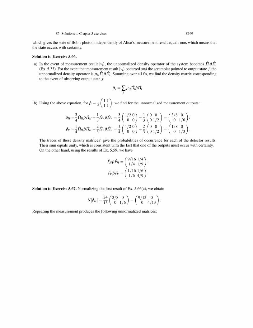
Solution to Exercise 5.66.
a) In the event of measurement result |vi〉, the unnormalized density operator of the system becomes ΠiρΠi(Ex. 5.33). For the event that measurement result |vi〉 occurred and the scrambler pointed to output state j, theunnormalized density operator is µi jΠiρΠi. Summing over all i’s, we find the density matrix correspondingto the event of observing output state j:
ρ j = ∑i
µi jΠiρΠi.
b) Using the above equation, for ρ = 12
(1 11 1
), we find for the unnormalized measurement outputs:
ρH =34
ΠH ρΠH +13
ΠV ρΠV =34
(1/2 00 0
)+
13
(0 00 1/2
)=
(3/8 00 1/6
);
ρV =14
ΠH ρΠH +23
ΠV ρΠV =14
(1/2 00 0
)+
23
(0 00 1/2
)=
(1/8 00 1/3
).
The traces of these density matrices’ give the probabilities of occurrence for each of the detector results.Their sum equals unity, which is consistent with the fact that one of the outputs must occur with certainty.On the other hand, using the results of Ex. 5.59, we have
FH ρFH =
(9/16 1/41/4 1/9
);
FV ρFV =
(1/16 1/61/6 4/9
).
Solution to Exercise 5.67. Normalizing the first result of Ex. 5.66(a), we obtain
N[ρH ] =2413
(3/8 00 1/6
)=
(9/13 0
0 4/13
).
Repeating the measurement produces the following unnormalized matrices:
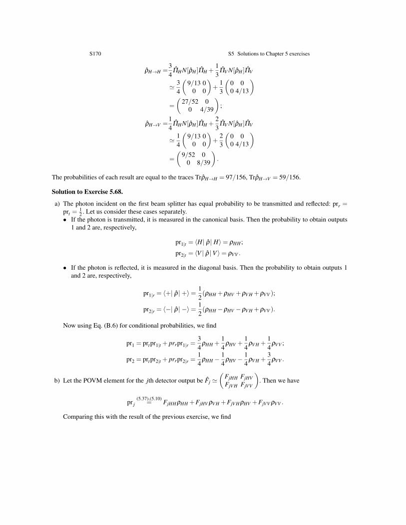
S170 S5 Solutions to Chapter 5 exercises
ρH→H =34
ΠHN[ρH ]ΠH +13
ΠV N[ρH ]ΠV
' 34
(9/13 0
0 0
)+
13
(0 00 4/13
)=
(27/52 0
0 4/39
);
ρH→V =14
ΠHN[ρH ]ΠH +23
ΠV N[ρH ]ΠV
' 14
(9/13 0
0 0
)+
23
(0 00 4/13
)=
(9/52 0
0 8/39
).
The probabilities of each result are equal to the traces TrρH→H = 97/156, TrρH→V = 59/156.
Solution to Exercise 5.68.
a) The photon incident on the first beam splitter has equal probability to be transmitted and reflected: prr =prt =
12 . Let us consider these cases separately.
• If the photon is transmitted, it is measured in the canonical basis. Then the probability to obtain outputs1 and 2 are, respectively,
pr1|t = 〈H| ρ| H〉= ρHH ;
pr2|t = 〈V | ρ|V 〉= ρVV .
• If the photon is reflected, it is measured in the diagonal basis. Then the probability to obtain outputs 1and 2 are, respectively,
pr1|r = 〈+| ρ|+〉=12(ρHH +ρHV +ρV H +ρVV );
pr2|r = 〈−| ρ| −〉=12(ρHH −ρHV −ρV H +ρVV ).
Now using Eq. (B.6) for conditional probabilities, we find
pr1 = prtpr1|t + prrpr1|r =34
ρHH +14
ρHV +14
ρV H +14
ρVV ;
pr2 = prtpr2|t + prrpr2|r =14
ρHH −14
ρHV −14
ρV H +34
ρVV .
b) Let the POVM element for the jth detector output be Fj '(
FjHH FjHVFjV H FjVV
). Then we have
pr j(5.37),(5.10)
= FjHHρHH +FjHV ρV H +FjV HρHV +FjVV ρVV .
Comparing this with the result of the previous exercise, we find
S5 Solutions to Chapter 5 exercises S171
F1 '(
3/4 1/41/4 1/4
); F2 '
(1/4 −1/4−1/4 3/4
).
As expected, F1 + F2 = 1.
Solution to Exercise 5.69.
a) We rely on the fact that probability (5.37) is a real number for any physical state ρ . Let us first set ρ =|vk〉〈vk|, where |vk〉 is an arbitrary orthonormal basis of the Hilbert space. We then have
Tr(Fjρ) =⟨vk∣∣ Fj∣∣ vk⟩∈ R,
which shows that all diagonal elements (Fj)kk of the matrix of Fj are real. Next, let us prove that anyoff-diagonal elements (Fj)kl and (Fj)lk are complex conjugate of each other. Consider states ρre,im =∣∣ψre,im
⟩⟨ψre,im
∣∣ with ψre = (|vk〉+ |vl〉)/√
2 and ψim = (|vk〉+ i |vl〉)/√
2. For these states, (ρre,im)kk =
(ρre,im)ll = (ρre)kl = (ρre)lk =12 , (ρim)kl =− i
2 , and (ρim)lk =i2 . Hence
Tr[Fj |ψre〉〈ψre|] =12[(Fj)kk +(Fj)ll +(Fj)kl +(Fj)lk] ∈ R;
Tr[Fj |ψim〉〈ψre|] =12[(Fj)kk +(Fj)ll ]+
i2[(Fj)kl− (Fj)lk] ∈ R.
Because, as we found out, both (Fj)kk and (Fj)ll are real, it follows from the above that
Im [(Fj)kl +(Fj)lk] = 0;Re [(Fj)kl− (Fj)lk] = 0.
This means that Im(Fj)kl =−Im(Fj)lk and Re(Fj)kl = Re(Fj)lk, i.e. (Fj)kl = (Fj)∗lk.
b) Suppose a POVM element Fj is not non-negative, i.e. there exists a state |ψ〉 such that⟨ψ∣∣ Fj∣∣ ψ⟩< 0.
But this value, according to Eq. (5.37), equals the probability pr j = Tr(Fj |ψ〉〈ψ|) of observing the jthdetector output when measuring state |ψ〉. Because negative probabilities are impossible, we have arrived ata contradiction.
c) Suppose we perform a measurement on a physical state with density matrix ρ . Because this measurementwill with certainty result in exactly one output state of the detector, we can write using Eq. (5.37):
∑j
pr j = ∑j
Tr(Fjρ) = Tr(X ρ) = 1, (S5.21)
where we denoted ∑ j Fj = X .Because all Fj are Hermitian operators, so is X . Hence there exists an orthonormal basis |vk〉 in which Xdiagonalizes (see Ex. A.60). Setting ρ = |vk〉〈vk| and substituting this state into Eq. (S5.21), we then have
Tr(X ρ) =⟨vk∣∣ X∣∣ vk⟩= 1.
Because the matrix of X is diagonal in basis |vk〉, it follows from the above relation that this matrixcorresponds to the identity operator.
S172 S5 Solutions to Chapter 5 exercises
Solution to Exercise 5.70. For any POVM element Fj, there exists an orthonormal basis |vi〉 in which Fj diag-onalizes. Substituting elements of this basis into Eq. (5.37), we find for the probability of the jth measurementoutcome
pr j = Tr(Fj |vi〉〈vi|) =⟨vi∣∣ Fj∣∣ vi⟩.
The detector’s not being able to provide information about the system’s quantum state means that p j is the samefor all input states, so
⟨vi∣∣ Fj∣∣ vi⟩
is the same for all values of i. In other words, the matrix of Fj in basis |vi〉 isdiagonal with all diagonal elements equal to p j.
Solution to Exercise 5.71.
a) The density matrix contains N2 elements, which implies that N2 complex parameters suffice to fully describeit. However, since the density operator is Hermitian, ρi j = ρ∗ji, so one pair of real numbers provides infor-mation about both these matrix elements (and only one real number is required for each diagonal element).Hence N2 real parameters are in fact sufficient. Furthemore, physical density matrices have the unity tracerestriction, which means that if we know any N− 1 diagonal elements, we can calculate the Nth one. Thisfurther reduces the number of needed real parameters to N2−1.Note that physical density matrices are also restricted by condition (5.3). However, this condition is aninequality and hence does not further reduce the number of required parameters.
b) Projective measurements in a given basis ∣∣v j⟩ yield N real probabilities pr j =
⟨v j∣∣ ρ∣∣ v j⟩
associated withthe N basis elements. However, because these probabilities add up to one, the information about them canbe contained in N−1 real numbers.
Solution to Exercise 5.72. Using the results of Exercise 5.3, we find
ρVV = prH ;ρVV = prV ;
ρHV +ρV H = 2pr+−prH −prV = 2pr+−1;ρHV −ρV H =−i(2prR−prH −prV ) =−i(2prR−1),
where we used prH +prV = 1. The latter two equations give
ρHV = pr+− iprR +−1+ i
2;
ρHV = pr++ iprR +−1− i
2.
Solution to Exercise 5.73. We look for the two photons’ density matrix in the canonical basis
ρ '
ρHHHH ρHHHV ρHHV H ρHHVVρHV HH ρHV HV ρHVV H ρHVVVρV HHH ρV HHV ρV HV H ρV HVVρVV HH ρVV HV ρVVV H ρVVVV
,
where e.g. ρHHHV = 〈HH| ρ| HV 〉.
S5 Solutions to Chapter 5 exercises S173
• Measurements in Alice’s and Bob’s canonical bases yield the diagonal elements
prHH = 〈HH| ρ| HH〉= ρHHHH ;prHV = 〈HV | ρ| HV 〉= ρHV HV ;prV H = 〈V H| ρ|V H〉= ρV HV H ;prVV = 〈VV | ρ|VV 〉= ρVVVV .
• Measurements in which Alice’s basis is canonical and Bob’s diagonal and circular yield
prH+ =12[〈H|⊗ (〈H|+ 〈V |)
]ρ[|H〉⊗ (|H〉+ |V 〉)
]=
12(ρHHHH +ρHHHV +ρHV HH +ρHV HV );
prHR =12[〈H|⊗ (〈H|− i〈V |)
]ρ[|H〉⊗ (|H〉+ i |V 〉)
]=
12(ρHHHH + iρHHHV − iρHV HH +ρHV HV ),
from which, using the existing knowledge of ρHHHH and ρHV HV , we find ρHHHV ±ρHV HH and, subsequently,both ρHHHV and ρHV HH . Similarly, from prV+ and prV R we find ρVVV H and ρV HVV .
• Measurements in which Bob’s basis is canonical and Alice’s diagonal and circular yield, by the same token,ρHHV H , ρV HHH , ρVV HV and ρHVVV .
• The matrix elements that remain to be found are ρHHVV , ρVV HH , ρHVV H and ρV HHV . We can calculate themby from measurements in which Alice’s and Bob’s bases are diagonal and circular. In particular,
pr++ =12[(〈H|+ 〈V |)⊗ (〈H|+ 〈V |)
]ρ[(|H〉+ |V 〉)⊗ (|H〉+ |V 〉)
]=
14(. . .+ρHHVV +ρVV HH +ρHVV H +ρV HHV + . . .);
pr+R =12[(〈H|+ 〈V |)⊗ (〈H|− i〈V |)
]ρ[(|H〉+ |V 〉)⊗ (|H〉+ i |V 〉)
]=
14(. . .+ iρHHVV − iρVV HH − iρHVV H + iρV HHV + . . .);
prR+ =12[(〈H|− i〈V |)⊗ (〈H|+ 〈V |)
]ρ[(|H〉+ i |V 〉)⊗ (|H〉+ |V 〉)
]=
14(. . .+ iρHHVV − iρVV HH + iρHVV H − iρV HHV + . . .);
prRR =12[(〈H|− i〈V |)⊗ (〈H|− i〈V |)
]ρ[(|H〉+ i |V 〉)⊗ (|H〉+ i |V 〉)
]=
14(. . .−ρHHVV −ρVV HH +ρHVV H +ρV HHV + . . .),
where the ellipses stand for those density matrix elements that are known from previous steps. The above fourequations can be readily solved to find the four remaining unknown matrix elements.
S174 S5 Solutions to Chapter 5 exercises
Solution to Exercise 5.74. As found in Ex. 5.22(b), E(ρ) = U ρU†. The matrix of E(ρ) in basis |vi〉 istherefore simply the product of matrices U , ρ and U†.
Solution to Exercise 5.75. As we found in Ex. 5.21(a), state αρ1 +βρ2 is equivalent, in all its physical prop-erties, to the ensemble in which state ρ1 occurs with probability α , and state ρ2 with probability β . So wecan, without loss of generality, assume that it is the ensemble entering the “black box”. After passing through the“black box”, states ρ1,2 produce states E(ρ1,2), respectively. Therefore, the output has an ensemble in which stateE(ρ1) occurs with probability α , and state E(ρ2) with probability β . This is equivalent to αE(ρ1)+βE(ρ2).
Solution to Exercise 5.76. By construction, each element in Q (the set defined in the Hint to this Exercise)corresponds to a physical state. The number of elements in Q is N2. According to Ex. A.7, all that needs to beproven to demonstrate that Q is a basis is that it forms a spanning set in the space of linear operators.
To this end, we express operator |vk〉〈vl |, for any k and l, through the elements of Q. For k = l, this expressionis trivial |vk〉〈vl |= ρkk. For k 6= l we write
ρre,kl =12(ρkk + ρll + |vk〉〈vl |+ |vl〉〈vk|);
ρim,kl =12(ρkk + ρll− i |vk〉〈vl |+ i |vl〉〈vk|),
from which it follows that
|vk〉〈vl |= ρre,kl + iρim,kl−1+ i
2(ρkk + ρll);
|vl〉〈vk|= ρre,kl− iρim,kl−1− i
2(ρkk + ρll).
Because set |vk〉〈vl | forms a basis in the space of linear operators (see Ex. A.42), so does Q.
Solution to Exercise 5.77. The statement of this exercise is a direct generalization of Ex. 5.75.
Solution to Exercise 5.78. The verification of linear independence of the setρ↑ '
(1 00 0
), ρ↓ '
(0 00 1
), ρ+ '
12
(1 11 1
), ρR '
12
(1 −ii 1
). (S5.22)
is straightforward. Let us check that Q is also a spanning set. We need to find the coefficients of decomposition
ρ = λ↑ρ↑+λ↓ρ↓+λ+ρ++λRρR,
which we can rewrite in the matrix form as(ρ↑↑ ρ↑↓ρ↓↑ ρ↓↓
)=
(λ↑+
12 (λ++λR)
12 (λ+− iλR)
12 (λ++ iλR) λ↓+
12 (λ++λR)
).
Solving the above equation for the λ ’s, we find
S5 Solutions to Chapter 5 exercises S175
λ+ = ρ↑↓+ρ↓↑;λR = i(ρ↑↓−ρ↓↑);
λ↑ = ρ↑↑−1+ i
2ρ↑↓−
1− i2
ρ↓↑;
λ↓ = ρ↓↓−1+ i
2ρ↑↓−
1− i2
ρ↓↑. (S5.23)
or
ρ '(
ρ↑↑−1+ i
2ρ↑↓−
1− i2
ρ↓↑
)ρ↑ (S5.24)
+
(ρ↓↓−
1+ i2
ρ↑↓−1− i
2ρ↓↑
)ρ↓
+(ρ↑↓+ρ↓↑)ρ++ i(ρ↑↓−ρ↓↑)ρR.
We see that a decomposition into the elements of Q exists for every ρ , so Q is indeed a spanning set.
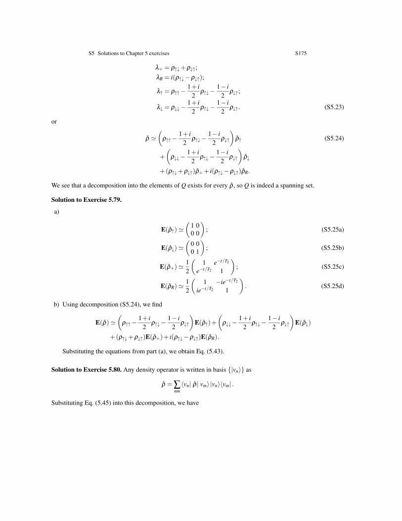
Solution to Exercise 5.79.
a)
E(ρ↑)'(
1 00 0
); (S5.25a)
E(ρ↓)'(
0 00 1
); (S5.25b)
E(ρ+)'12
(1 e−t/T2
e−t/T2 1
); (S5.25c)
E(ρR)'12
(1 −ie−t/T2
ie−t/T2 1
). (S5.25d)
b) Using decomposition (S5.24), we find
E(ρ)'(
ρ↑↑−1+ i
2ρ↑↓−
1− i2
ρ↓↑
)E(ρ↑)+
(ρ↓↓−
1+ i2
ρ↑↓−1− i
2ρ↓↑
)E(ρ↓)
+(ρ↑↓+ρ↓↑)E(ρ+)+ i(ρ↑↓−ρ↓↑)E(ρR).
Substituting the equations from part (a), we obtain Eq. (5.43).
Solution to Exercise 5.80. Any density operator is written in basis |vn〉 as
ρ = ∑nm〈vn| ρ| vm〉 |vn〉〈vm| .
Substituting Eq. (5.45) into this decomposition, we have
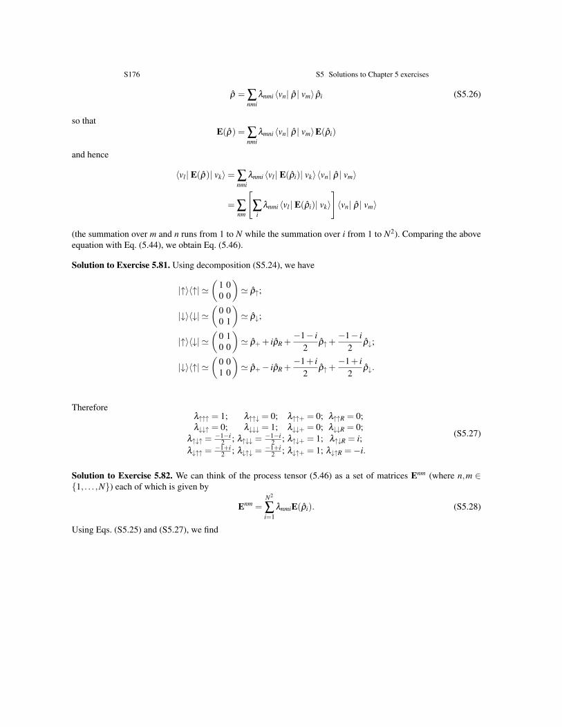
S176 S5 Solutions to Chapter 5 exercises
ρ = ∑nmi
λnmi 〈vn| ρ| vm〉 ρi (S5.26)
so thatE(ρ) = ∑
nmiλmni 〈vn| ρ| vm〉E(ρi)
and hence
〈vl | E(ρ)| vk〉= ∑nmi
λnmi 〈vl | E(ρi)| vk〉〈vn| ρ| vm〉
= ∑nm
[∑
iλnmi 〈vl | E(ρi)| vk〉
]〈vn| ρ| vm〉
(the summation over m and n runs from 1 to N while the summation over i from 1 to N2). Comparing the aboveequation with Eq. (5.44), we obtain Eq. (5.46).
Solution to Exercise 5.81. Using decomposition (S5.24), we have
|↑〉〈↑| '(
1 00 0
)' ρ↑;
|↓〉〈↓| '(
0 00 1
)' ρ↓;
|↑〉〈↓| '(
0 10 0
)' ρ++ iρR +
−1− i2
ρ↑+−1− i
2ρ↓;
|↓〉〈↑| '(
0 01 0
)' ρ+− iρR +
−1+ i2
ρ↑+−1+ i
2ρ↓.
Thereforeλ↑↑↑ = 1; λ↑↑↓ = 0; λ↑↑+ = 0; λ↑↑R = 0;λ↓↓↑ = 0; λ↓↓↓ = 1; λ↓↓+ = 0; λ↓↓R = 0;
λ↑↓↑ =−1−i
2 ; λ↑↓↓ =−1−i
2 ; λ↑↓+ = 1; λ↑↓R = i;λ↓↑↑ =
−1+i2 ; λ↓↑↓ =
−1+i2 ; λ↓↑+ = 1; λ↓↑R =−i.
(S5.27)
Solution to Exercise 5.82. We can think of the process tensor (5.46) as a set of matrices Enm (where n,m ∈1, . . . ,N) each of which is given by
Enm =N2
∑i=1
λnmiE(ρi). (S5.28)
Using Eqs. (S5.25) and (S5.27), we find
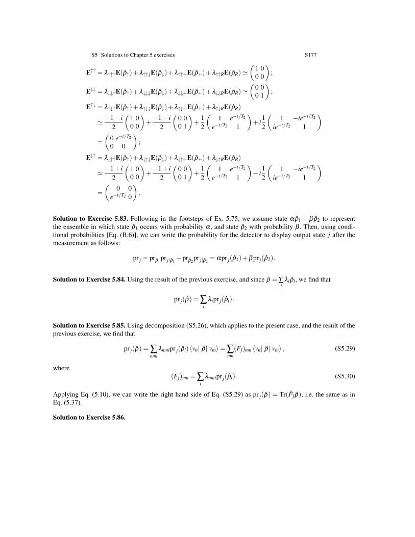
S5 Solutions to Chapter 5 exercises S177
E↑↑ = λ↑↑↑E(ρ↑)+λ↑↑↓E(ρ↓)+λ↑↑+E(ρ+)+λ↑↑RE(ρR)'(
1 00 0
);
E↓↓ = λ↓↓↑E(ρ↑)+λ↓↓↓E(ρ↓)+λ↓↓+E(ρ+)+λ↓↓RE(ρR)'(
0 00 1
);
E↑↓ = λ↑↓↑E(ρ↑)+λ↑↓↓E(ρ↓)+λ↑↓+E(ρ+)+λ↑↓RE(ρR)
' −1− i2
(1 00 0
)+−1− i
2
(0 00 1
)+
12
(1 e−t/T2
e−t/T2 1
)+ i
12
(1 −ie−t/T2
ie−t/T2 1
)=
(0 e−t/T2
0 0
);
E↓↑ = λ↓↑↑E(ρ↑)+λ↓↑↓E(ρ↓)+λ↓↑+E(ρ+)+λ↓↑RE(ρR)
' −1+ i2
(1 00 0
)+−1+ i
2
(0 00 1
)+
12
(1 e−t/T2
e−t/T2 1
)− i
12
(1 −ie−t/T2
ie−t/T2 1
)=
(0 0
e−t/T2 0
).
Solution to Exercise 5.83. Following in the footsteps of Ex. 5.75, we assume state αρ1 + βρ2 to representthe ensemble in which state ρ1 occurs with probability α , and state ρ2 with probability β . Then, using condi-tional probabilities [Eq. (B.6)], we can write the probability for the detector to display output state j after themeasurement as follows:
pr j = prρ1pr j|ρ1
+prρ2pr j|ρ2
= αpr j(ρ1)+βpr j(ρ2).
Solution to Exercise 5.84. Using the result of the previous exercise, and since ρ = ∑i
λiρi, we find that
pr j(ρ) = ∑i
λipr j(ρi).
Solution to Exercise 5.85. Using decomposition (S5.26), which applies to the present case, and the result of theprevious exercise, we find that
pr j(ρ) = ∑nmi
λnmipr j(ρi)〈vn| ρ| vm〉= ∑nm(Fj)mn 〈vn| ρ| vm〉 , (S5.29)
where(Fj)mn = ∑
iλnmipr j(ρi). (S5.30)
Applying Eq. (5.10), we can write the right-hand side of Eq. (S5.29) as pr j(ρ) = Tr(Fjρ), i.e. the same as inEq. (5.37).
Solution to Exercise 5.86.
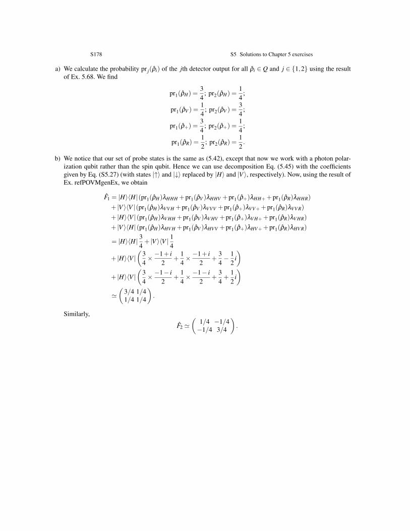
S178 S5 Solutions to Chapter 5 exercises
a) We calculate the probability pr j(ρi) of the jth detector output for all ρi ∈ Q and j ∈ 1,2 using the resultof Ex. 5.68. We find
pr1(ρH) =34
; pr2(ρH) =14
;
pr1(ρV ) =14
; pr2(ρV ) =34
;
pr1(ρ+) =34
; pr2(ρ+) =14
;
pr1(ρR) =12
; pr2(ρR) =12.
b) We notice that our set of probe states is the same as (5.42), except that now we work with a photon polar-ization qubit rather than the spin qubit. Hence we can use decomposition Eq. (5.45) with the coefficientsgiven by Eq. (S5.27) (with states |↑〉 and |↓〉 replaced by |H〉 and |V 〉, respectively). Now, using the result ofEx. refPOVMgenEx, we obtain
F1 = |H〉〈H|(pr1(ρH)λHHH +pr1(ρV )λHHV +pr1(ρ+)λHH++pr1(ρR)λHHR)
+ |V 〉〈V |(pr1(ρH)λVV H +pr1(ρV )λVVV +pr1(ρ+)λVV++pr1(ρR)λVV R)
+ |H〉〈V |(pr1(ρH)λV HH +pr1(ρV )λV HV +pr1(ρ+)λV H++pr1(ρR)λV HR)
+ |V 〉〈H|(pr1(ρH)λHV H +pr1(ρV )λHVV +pr1(ρ+)λHV++pr1(ρR)λHV R)
= |H〉〈H| 34+ |V 〉〈V | 1
4
+ |H〉〈V |(
34× −1+ i
2+
14× −1+ i
2+
34− 1
2i)
+ |H〉〈V |(
34× −1− i
2+
14× −1− i
2+
34+
12
i)
'(
3/4 1/41/4 1/4
).
Similarly,
F2 '(
1/4 −1/4−1/4 3/4
).