Appendix B Overview in Probability and Random Processes
53
Appendix B Overview in Probability and Random Processes Po-Ning Chen, Professor Institute of Communications Engineering National Chiao Tung University Hsin Chu, Taiwan 30010, R.O.C.
Transcript of Appendix B Overview in Probability and Random Processes
Appendix B
Overview in Probability and RandomProcesses
Po-Ning Chen, Professor
Institute of Communications Engineering
National Chiao Tung University
Hsin Chu, Taiwan 30010, R.O.C.
B.1 Probability space I: b-1
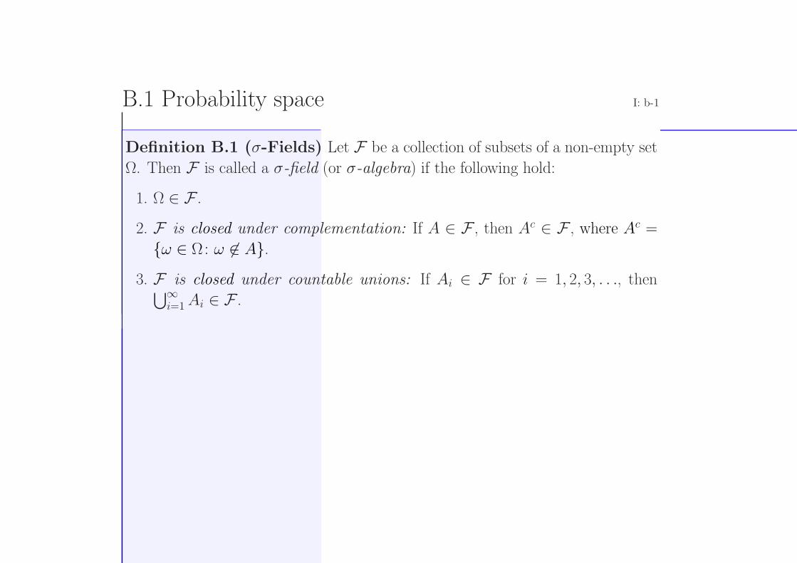
Definition B.1 (σ-Fields) Let F be a collection of subsets of a non-empty set
Ω. Then F is called a σ-field (or σ-algebra) if the following hold:
1. Ω ∈ F .
2. F is closed under complementation: If A ∈ F , then Ac ∈ F , where Ac =
ω ∈ Ω: ω ∈ A.3. F is closed under countable unions: If Ai ∈ F for i = 1, 2, 3, . . ., then⋃∞
i=1Ai ∈ F .
B.1 Probability space I: b-2
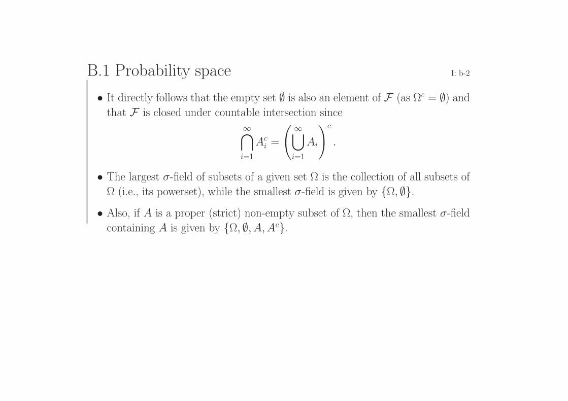
• It directly follows that the empty set ∅ is also an element of F (as Ωc = ∅) andthat F is closed under countable intersection since
∞⋂i=1
Aci =
( ∞⋃i=1
Ai
)c
.
• The largest σ-field of subsets of a given set Ω is the collection of all subsets of
Ω (i.e., its powerset), while the smallest σ-field is given by Ω, ∅.• Also, if A is a proper (strict) non-empty subset of Ω, then the smallest σ-field
containing A is given by Ω, ∅, A,Ac.
B.1 Probability space I: b-3
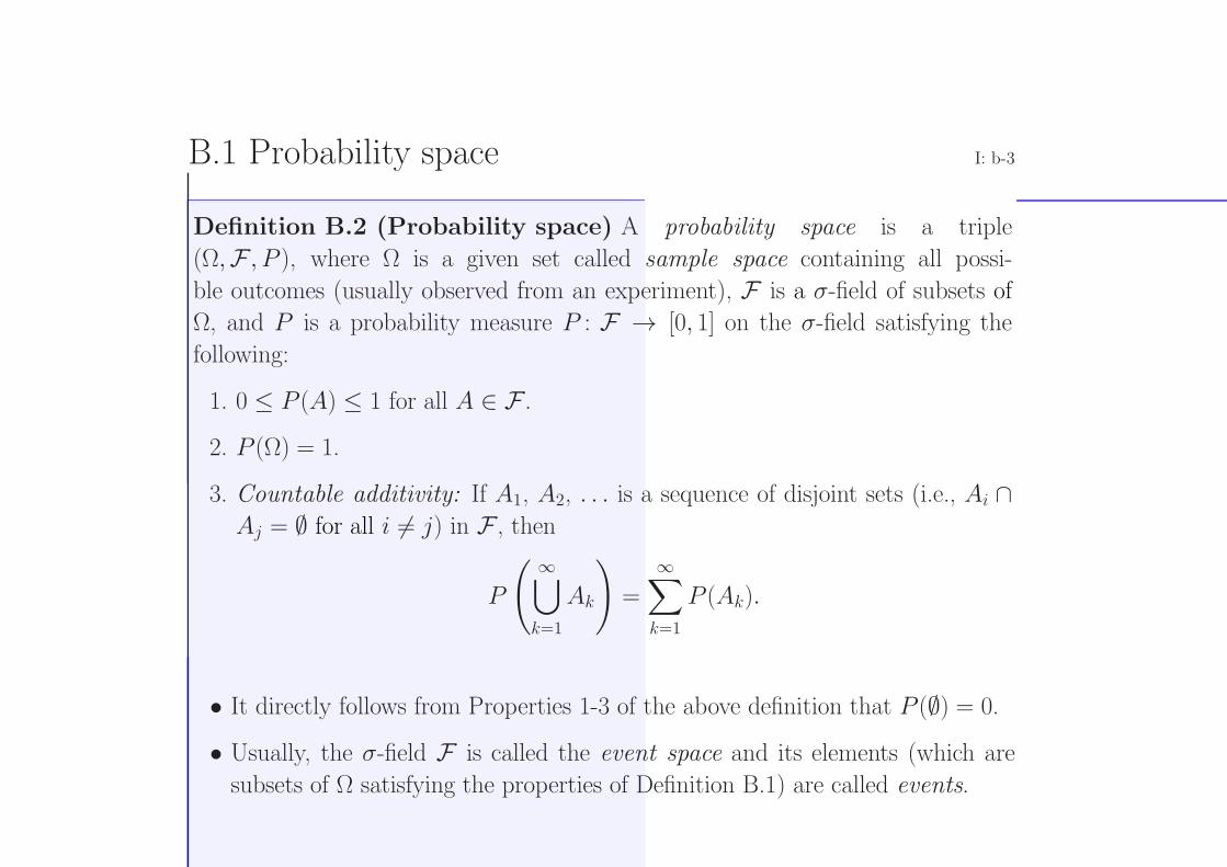
Definition B.2 (Probability space) A probability space is a triple
(Ω,F , P ), where Ω is a given set called sample space containing all possi-
ble outcomes (usually observed from an experiment), F is a σ-field of subsets of
Ω, and P is a probability measure P : F → [0, 1] on the σ-field satisfying the
following:
1. 0 ≤ P (A) ≤ 1 for all A ∈ F .
2. P (Ω) = 1.
3. Countable additivity: If A1, A2, . . . is a sequence of disjoint sets (i.e., Ai ∩Aj = ∅ for all i = j) in F , then
P
( ∞⋃k=1
Ak
)=
∞∑k=1
P (Ak).
• It directly follows from Properties 1-3 of the above definition that P (∅) = 0.
• Usually, the σ-field F is called the event space and its elements (which are
subsets of Ω satisfying the properties of Definition B.1) are called events.
B.1 Probability space I: b-4
• The Borel σ-field of R, denoted by B(R), is the smallest σ-field of subsets of
R containing all open intervals in R.
• The elements of B(R) are called Borel sets.
• For any random variable X , we use PX to denote the probability distribution
on B(R) induced by X , given by
PX(B) := Pr[X ∈ B] = P (w ∈ Ω : X(w) ∈ B) , B ∈ B(R).
Note that the quantities PX(B), B ∈ B(R), fully characterize the random
variable X as they determine the probabilities of all events that concern X .
B.2 Random variables and random processes I: b-5
• A random variable X defined over probability space (Ω,F , P ) is a real-valued
function X : Ω → R that is measurable (or F-measurable), i.e., satisfying the
property that
X−1((−∞, t]) := ω ∈ Ω : X(ω) ≤ t ∈ Ffor each real t.
• A random process (or random source) is a collection of random variables that
arise from the same probability space. It can be mathematically represented
by the collection
Xt, t ∈ I,where Xt denotes the t
th random variable in the process, and the index t runs
over an index set I which is arbitrary.
B.2 Random variables and random processes I: b-6
• The index set I can be uncountably infinite (e.g., I = R), in which case we are
dealing with a continuous-time process.
• Except for a brief interlude with the continuous-time (waveform) Gaussian
channel in Chapter 5, we will consider discrete-time communication systems
throughout the lectures.
To be precise, we will only consider the following cases of index set I :
case a) I consists of one index only.
case b) I is finite.
case c) I is countably infinite.
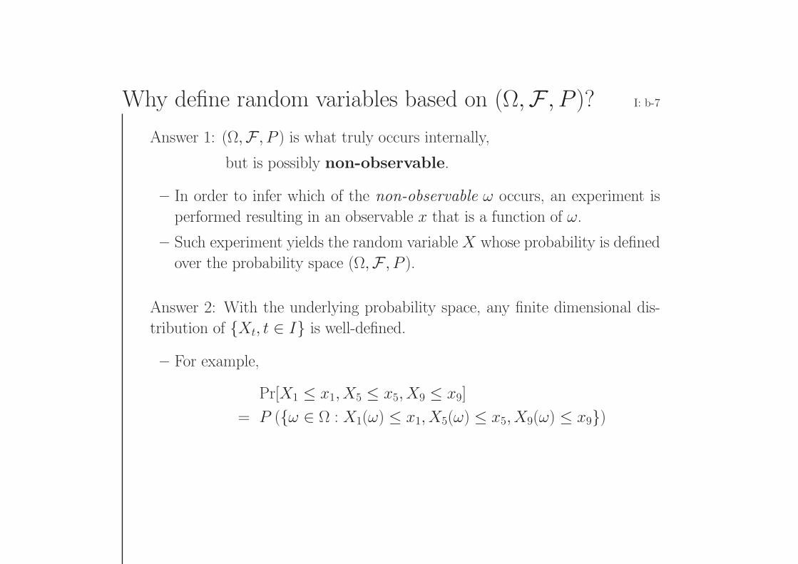
Why define random variables based on (Ω,F , P )? I: b-7
Answer 1: (Ω,F , P ) is what truly occurs internally,
but is possibly non-observable.
– In order to infer which of the non-observable ω occurs, an experiment is
performed resulting in an observable x that is a function of ω.
– Such experiment yields the random variable X whose probability is defined
over the probability space (Ω,F , P ).
Answer 2: With the underlying probability space, any finite dimensional dis-
tribution of Xt, t ∈ I is well-defined.
– For example,
Pr[X1 ≤ x1, X5 ≤ x5, X9 ≤ x9]
= P (ω ∈ Ω : X1(ω) ≤ x1, X5(ω) ≤ x5, X9(ω) ≤ x9)
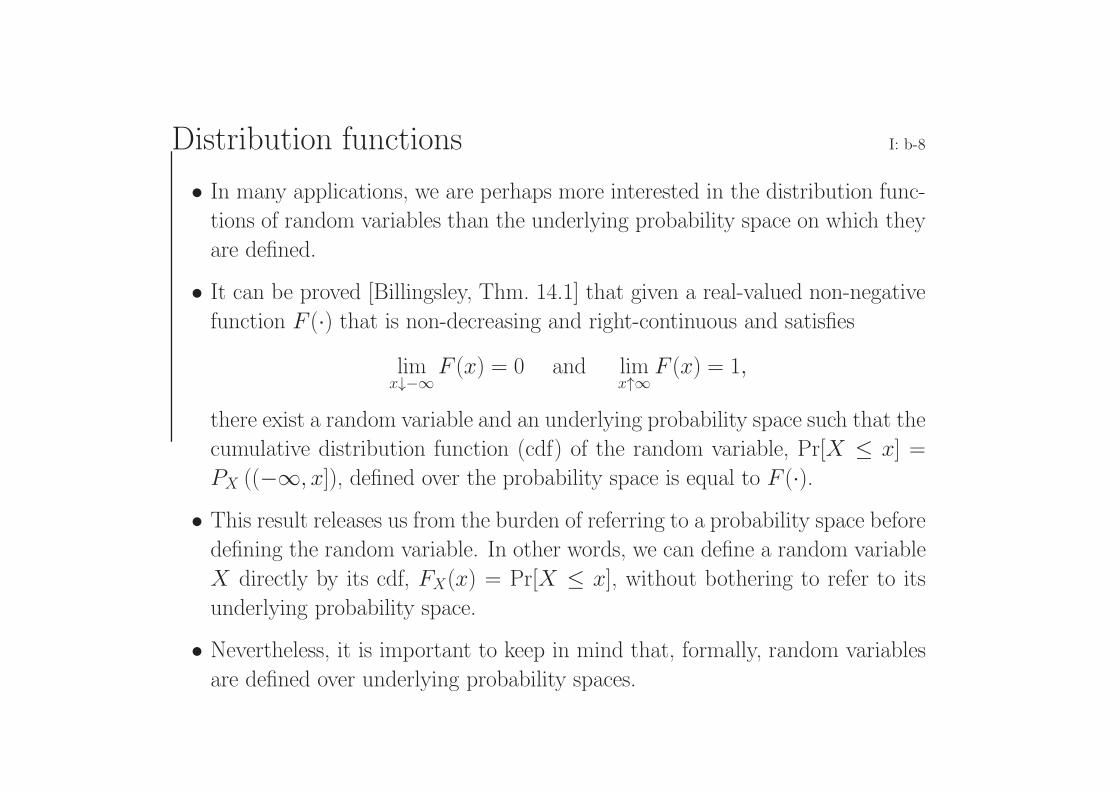
Distribution functions I: b-8
• In many applications, we are perhaps more interested in the distribution func-
tions of random variables than the underlying probability space on which they
are defined.
• It can be proved [Billingsley, Thm. 14.1] that given a real-valued non-negative
function F (·) that is non-decreasing and right-continuous and satisfies
limx↓−∞
F (x) = 0 and limx↑∞
F (x) = 1,
there exist a random variable and an underlying probability space such that the
cumulative distribution function (cdf) of the random variable, Pr[X ≤ x] =
PX ((−∞, x]), defined over the probability space is equal to F (·).• This result releases us from the burden of referring to a probability space before
defining the random variable. In other words, we can define a random variable
X directly by its cdf, FX(x) = Pr[X ≤ x], without bothering to refer to its
underlying probability space.
• Nevertheless, it is important to keep in mind that, formally, random variables
are defined over underlying probability spaces.
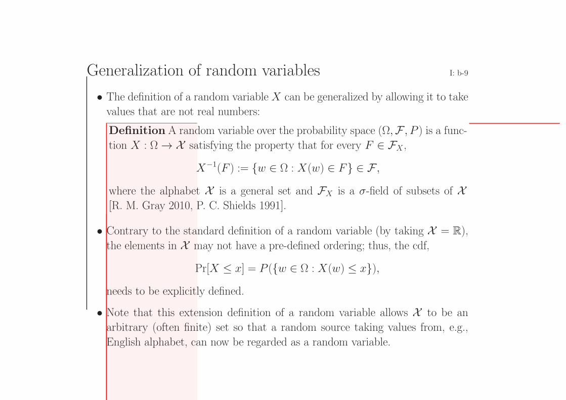
Generalization of random variables I: b-9
• The definition of a random variableX can be generalized by allowing it to take
values that are not real numbers:
Definition A random variable over the probability space (Ω,F , P ) is a func-
tion X : Ω → X satisfying the property that for every F ∈ FX ,
X−1(F ) := w ∈ Ω : X(w) ∈ F ∈ F ,
where the alphabet X is a general set and FX is a σ-field of subsets of X[R. M. Gray 2010, P. C. Shields 1991].
• Contrary to the standard definition of a random variable (by taking X = R),
the elements in X may not have a pre-defined ordering; thus, the cdf,
Pr[X ≤ x] = P (w ∈ Ω : X(w) ≤ x),needs to be explicitly defined.
• Note that this extension definition of a random variable allows X to be an
arbitrary (often finite) set so that a random source taking values from, e.g.,
English alphabet, can now be regarded as a random variable.
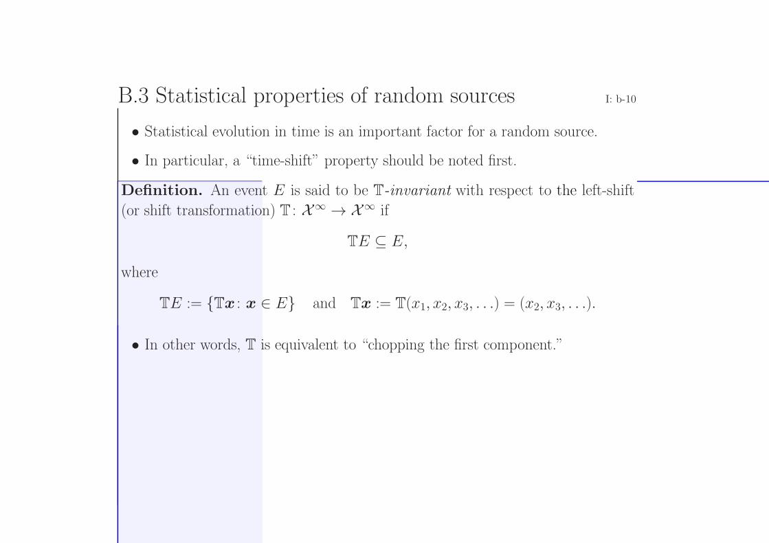
B.3 Statistical properties of random sources I: b-10
• Statistical evolution in time is an important factor for a random source.
• In particular, a “time-shift” property should be noted first.
Definition. An event E is said to be T-invariant with respect to the left-shift
(or shift transformation) T : X∞ → X∞ if
TE ⊆ E,
where
TE := Tx : x ∈ E and Tx := T(x1, x2, x3, . . .) = (x2, x3, . . .).
• In other words, T is equivalent to “chopping the first component.”
B.3 Statistical properties of random sources I: b-11
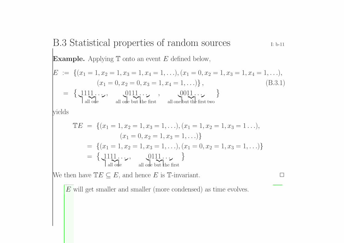
Example. Applying T onto an event E defined below,
E := (x1 = 1, x2 = 1, x3 = 1, x4 = 1, . . .), (x1 = 0, x2 = 1, x3 = 1, x4 = 1, . . .),
(x1 = 0, x2 = 0, x3 = 1, x4 = 1, . . .) , (B.3.1)
=
1111 . . .︸ ︷︷ ︸all one
, 0111 . . .︸ ︷︷ ︸all one but the first
, 0011 . . .︸ ︷︷ ︸all one but the first two
yields
TE = (x1 = 1, x2 = 1, x3 = 1, . . .), (x1 = 1, x2 = 1, x3 = 1 . . .),
(x1 = 0, x2 = 1, x3 = 1, . . .)= (x1 = 1, x2 = 1, x3 = 1, . . .), (x1 = 0, x2 = 1, x3 = 1, . . .)=
1111 . . .︸ ︷︷ ︸all one
, 0111 . . .︸ ︷︷ ︸all one but the first
We then have TE ⊆ E, and hence E is T-invariant.
E will get smaller and smaller (more condensed) as time evolves.
B.3 Statistical properties of random sources I: b-12
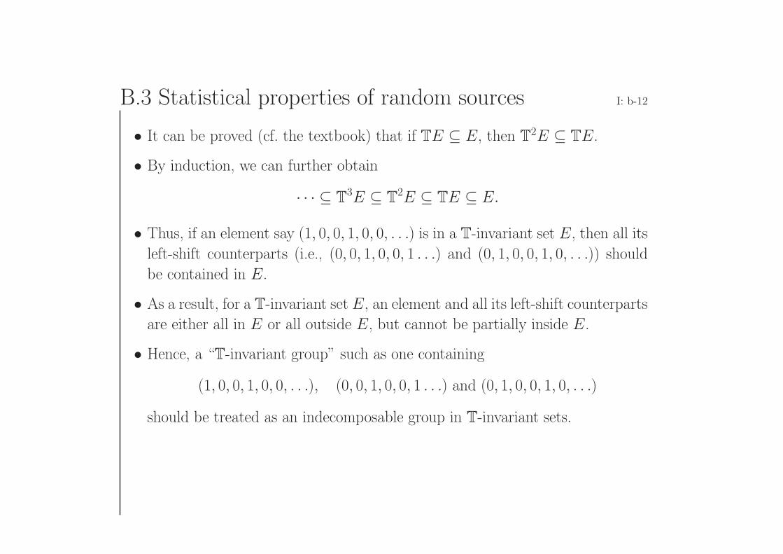
• It can be proved (cf. the textbook) that if TE ⊆ E, then T2E ⊆ TE.
• By induction, we can further obtain
· · · ⊆ T3E ⊆ T
2E ⊆ TE ⊆ E.
• Thus, if an element say (1, 0, 0, 1, 0, 0, . . .) is in a T-invariant set E, then all its
left-shift counterparts (i.e., (0, 0, 1, 0, 0, 1 . . .) and (0, 1, 0, 0, 1, 0, . . .)) should
be contained in E.
• As a result, for a T-invariant set E, an element and all its left-shift counterparts
are either all in E or all outside E, but cannot be partially inside E.
• Hence, a “T-invariant group” such as one containing
(1, 0, 0, 1, 0, 0, . . .), (0, 0, 1, 0, 0, 1 . . .) and (0, 1, 0, 0, 1, 0, . . .)
should be treated as an indecomposable group in T-invariant sets.
B.3 Statistical properties of random sources I: b-13
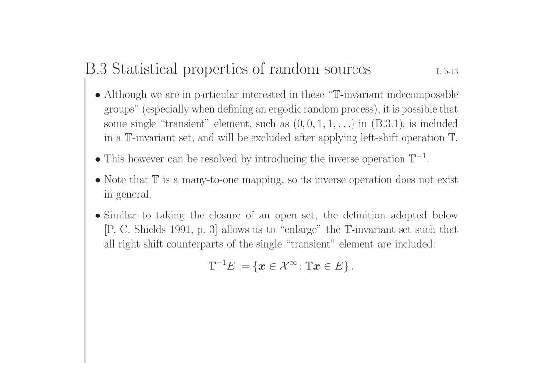
• Although we are in particular interested in these “T-invariant indecomposable
groups” (especially when defining an ergodic random process), it is possible that
some single “transient” element, such as (0, 0, 1, 1, . . .) in (B.3.1), is included
in a T-invariant set, and will be excluded after applying left-shift operation T.
• This however can be resolved by introducing the inverse operation T−1.
• Note that T is a many-to-one mapping, so its inverse operation does not exist
in general.
• Similar to taking the closure of an open set, the definition adopted below
[P. C. Shields 1991, p. 3] allows us to “enlarge” the T-invariant set such that
all right-shift counterparts of the single “transient” element are included:
T−1E := x ∈ X∞ : Tx ∈ E .
B.3 Statistical properties of random sources I: b-14
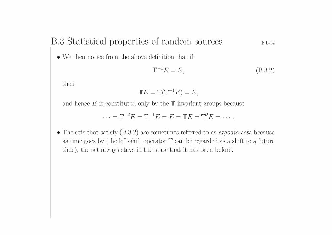
• We then notice from the above definition that if
T−1E = E, (B.3.2)
then
TE = T(T−1E) = E,
and hence E is constituted only by the T-invariant groups because
· · · = T−2E = T
−1E = E = TE = T2E = · · · .
• The sets that satisfy (B.3.2) are sometimes referred to as ergodic sets because
as time goes by (the left-shift operator T can be regarded as a shift to a future
time), the set always stays in the state that it has been before.
B.3 Statistical properties of random sources I: b-15
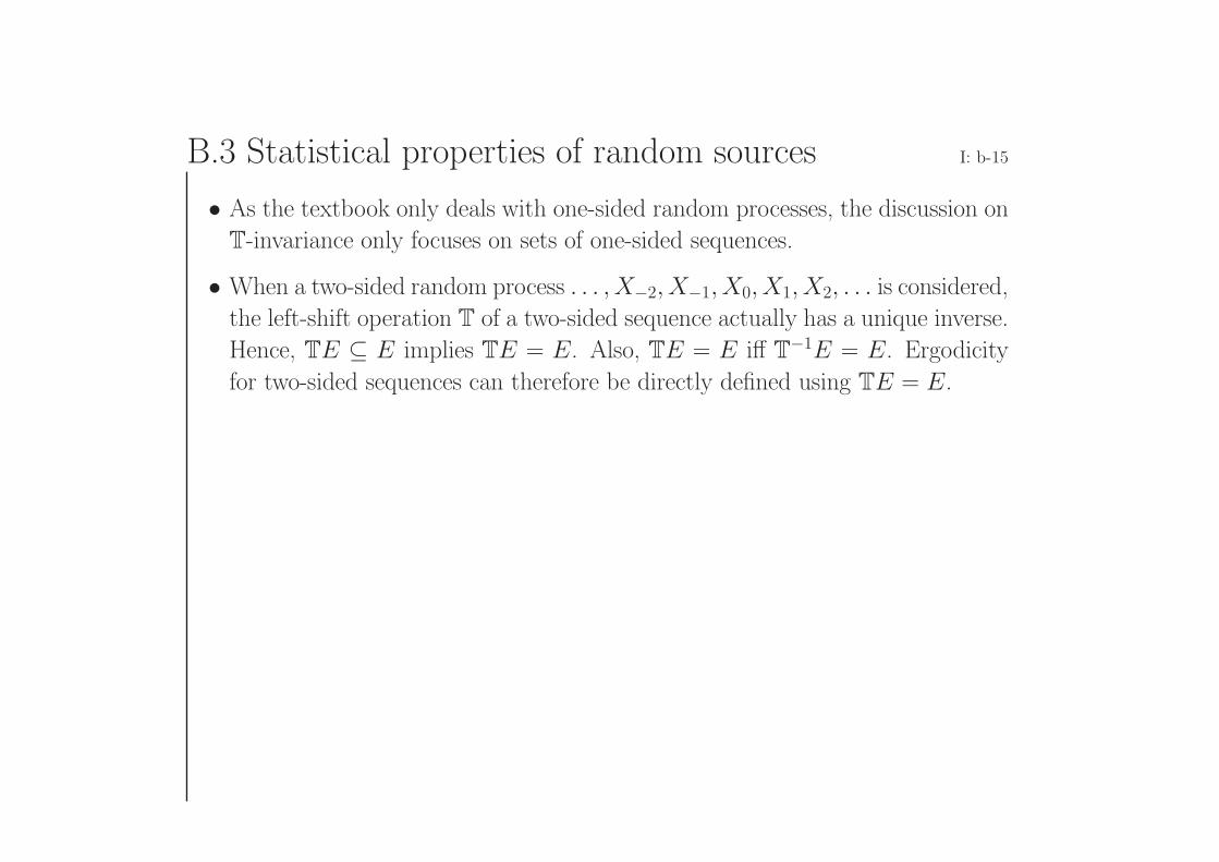
• As the textbook only deals with one-sided random processes, the discussion on
T-invariance only focuses on sets of one-sided sequences.
• When a two-sided random process . . . , X−2, X−1, X0, X1, X2, . . . is considered,
the left-shift operation T of a two-sided sequence actually has a unique inverse.
Hence, TE ⊆ E implies TE = E. Also, TE = E iff T−1E = E. Ergodicity
for two-sided sequences can therefore be directly defined using TE = E.
B.3 Statistical properties of random sources I: b-16
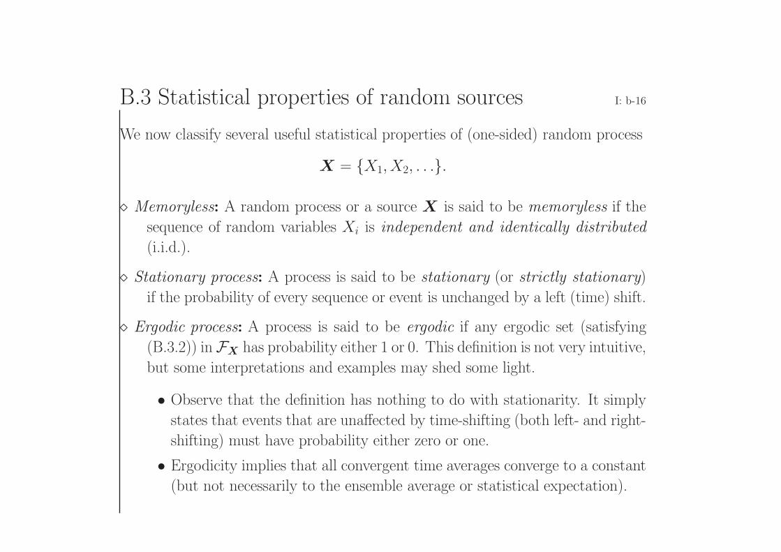
We now classify several useful statistical properties of (one-sided) random process
X = X1, X2, . . ..
Memoryless: A random process or a source X is said to be memoryless if the
sequence of random variables Xi is independent and identically distributed
(i.i.d.).
Stationary process: A process is said to be stationary (or strictly stationary)
if the probability of every sequence or event is unchanged by a left (time) shift.
Ergodic process: A process is said to be ergodic if any ergodic set (satisfying
(B.3.2)) inFX has probability either 1 or 0. This definition is not very intuitive,
but some interpretations and examples may shed some light.
• Observe that the definition has nothing to do with stationarity. It simply
states that events that are unaffected by time-shifting (both left- and right-
shifting) must have probability either zero or one.
• Ergodicity implies that all convergent time averages converge to a constant
(but not necessarily to the ensemble average or statistical expectation).
B.3 Statistical properties of random sources I: b-17
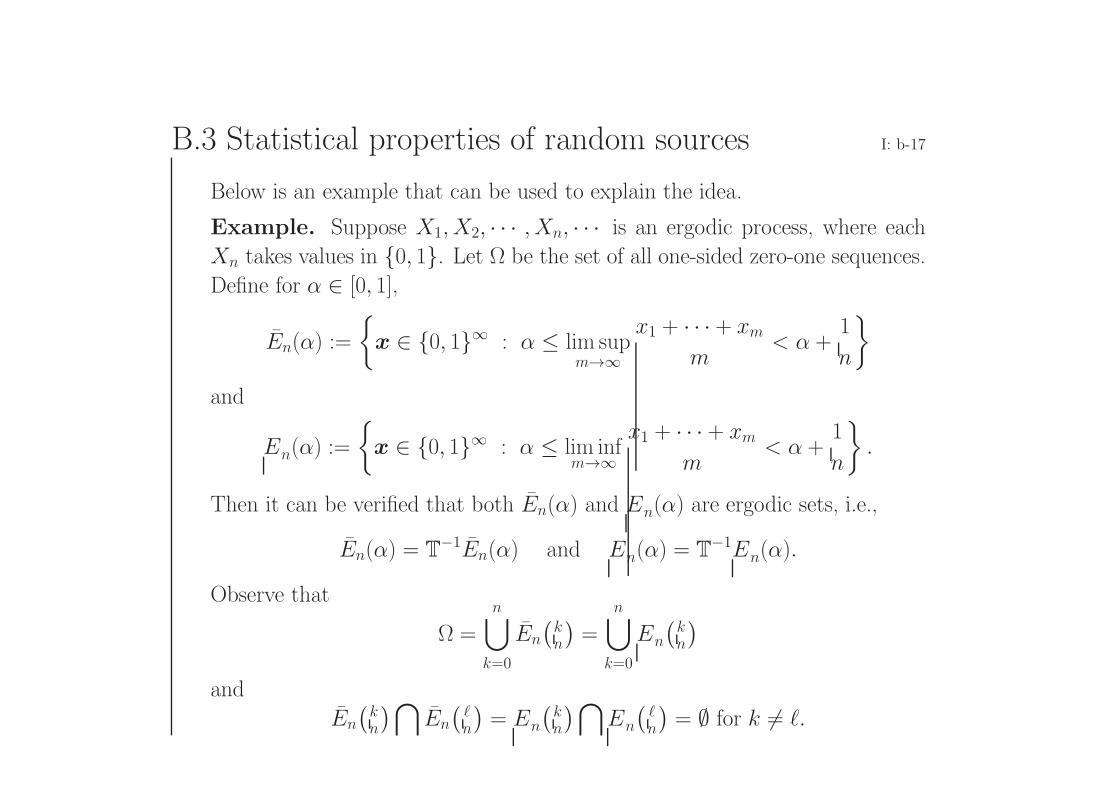
Below is an example that can be used to explain the idea.
Example. Suppose X1, X2, · · · , Xn, · · · is an ergodic process, where each
Xn takes values in 0, 1. Let Ω be the set of all one-sided zero-one sequences.
Define for α ∈ [0, 1],
En(α) :=
x ∈ 0, 1∞ : α ≤ lim sup
m→∞x1 + · · · + xm
m< α +
1
n
and
En(α) :=
x ∈ 0, 1∞ : α ≤ lim inf
m→∞x1 + · · · + xm
m< α +
1
n
.
Then it can be verified that both En(α) and En(α) are ergodic sets, i.e.,
En(α) = T−1En(α) and En(α) = T
−1En(α).
Observe that
Ω =
n⋃k=0
En
(kn
)=
n⋃k=0
En
(kn
)and
En
(kn
)⋂En
(n
)= En
(kn
)⋂En
(n
)= ∅ for k = .
B.3 Statistical properties of random sources I: b-18
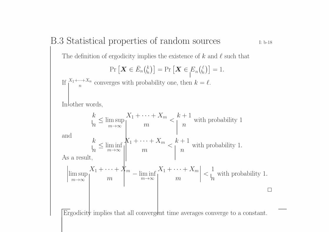
The definition of ergodicity implies the existence of k and such that
Pr[X ∈ En
(kn
)]= Pr
[X ∈ En
(n
)]= 1.
If X1+···+Xnn
converges with probability one, then k = .
In other words,
k
n≤ lim sup
m→∞X1 + · · · +Xm
m<
k + 1
nwith probability 1
andk
n≤ lim inf
m→∞X1 + · · · +Xm
m<
k + 1
nwith probability 1.
As a result,∣∣∣∣lim supm→∞
X1 + · · · +Xm
m− lim inf
m→∞X1 + · · · +Xm
m
∣∣∣∣ < 1
nwith probability 1.
Ergodicity implies that all convergent time averages converge to a constant.
B.3 Statistical properties of random sources I: b-19
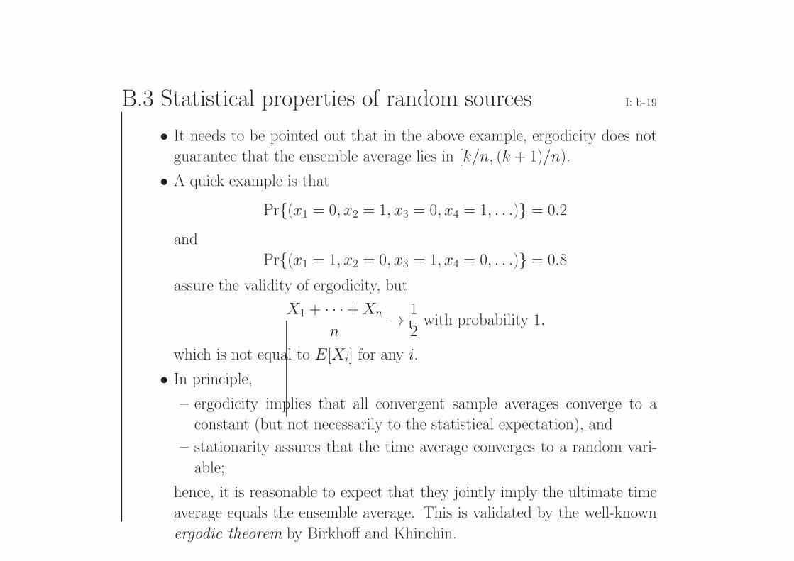
• It needs to be pointed out that in the above example, ergodicity does not
guarantee that the ensemble average lies in [k/n, (k + 1)/n).
• A quick example is that
Pr(x1 = 0, x2 = 1, x3 = 0, x4 = 1, . . .) = 0.2
and
Pr(x1 = 1, x2 = 0, x3 = 1, x4 = 0, . . .) = 0.8
assure the validity of ergodicity, but
X1 + · · · +Xn
n→ 1
2with probability 1.
which is not equal to E[Xi] for any i.
• In principle,
– ergodicity implies that all convergent sample averages converge to a
constant (but not necessarily to the statistical expectation), and
– stationarity assures that the time average converges to a random vari-
able;
hence, it is reasonable to expect that they jointly imply the ultimate time
average equals the ensemble average. This is validated by the well-known
ergodic theorem by Birkhoff and Khinchin.
B.3 Statistical properties of random sources I: b-20
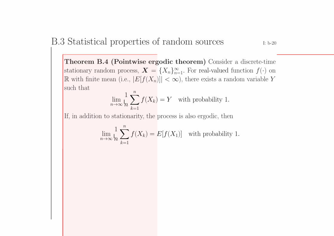
Theorem B.4 (Pointwise ergodic theorem) Consider a discrete-time
stationary random process, X = Xn∞n=1. For real-valued function f(·) onR with finite mean (i.e., |E[f(Xn)]| < ∞), there exists a random variable Y
such that
limn→∞
1
n
n∑k=1
f(Xk) = Y with probability 1.
If, in addition to stationarity, the process is also ergodic, then
limn→∞
1
n
n∑k=1
f(Xk) = E[f(X1)] with probability 1.
Operational meaning of stationary ergodic assumption I: b-21
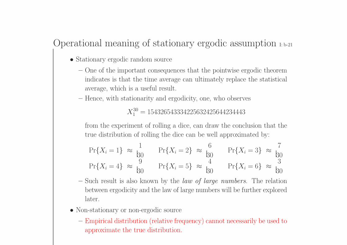
• Stationary ergodic random source
– One of the important consequences that the pointwise ergodic theorem
indicates is that the time average can ultimately replace the statistical
average, which is a useful result.
– Hence, with stationarity and ergodicity, one, who observes
X301 = 154326543334225632425644234443
from the experiment of rolling a dice, can draw the conclusion that the
true distribution of rolling the dice can be well approximated by:
PrXi = 1 ≈ 1
30PrXi = 2 ≈ 6
30PrXi = 3 ≈ 7
30
PrXi = 4 ≈ 9
30PrXi = 5 ≈ 4
30PrXi = 6 ≈ 3
30
– Such result is also known by the law of large numbers. The relation
between ergodicity and the law of large numbers will be further explored
later.
• Non-stationary or non-ergodic source
– Empirical distribution (relative frequency) cannot necessarily be used to
approximate the true distribution.
Operational meaning of stationary ergodic assumption I: b-22
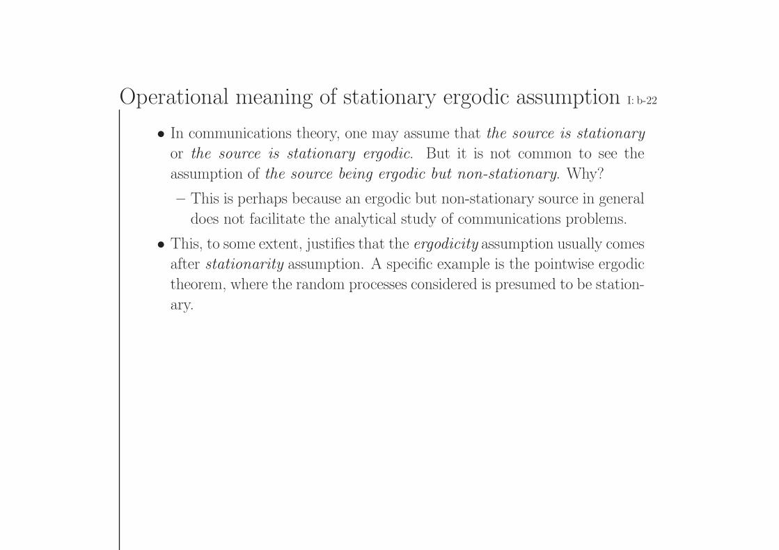
• In communications theory, one may assume that the source is stationary
or the source is stationary ergodic. But it is not common to see the
assumption of the source being ergodic but non-stationary. Why?
– This is perhaps because an ergodic but non-stationary source in general
does not facilitate the analytical study of communications problems.
• This, to some extent, justifies that the ergodicity assumption usually comes
after stationarity assumption. A specific example is the pointwise ergodic
theorem, where the random processes considered is presumed to be station-
ary.
B.3 Statistical properties of random sources I: b-23
We continue to classify useful statistical properties of (one-sided) random process
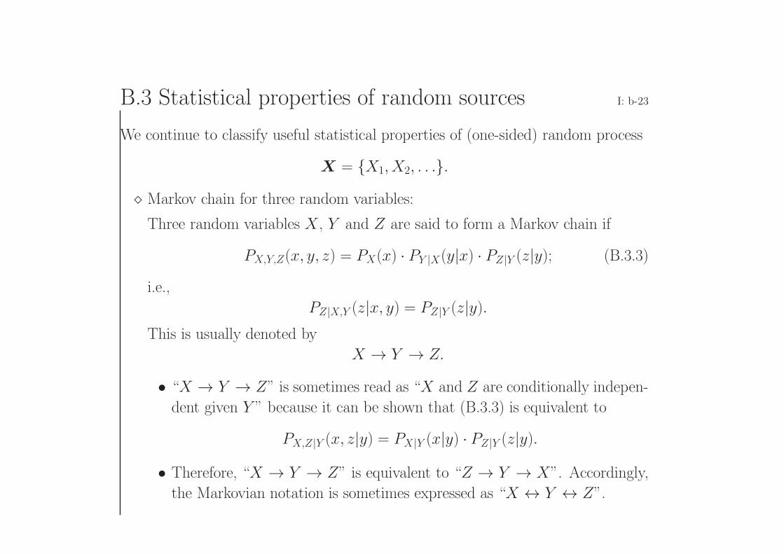
X = X1, X2, . . .. Markov chain for three random variables:
Three random variables X , Y and Z are said to form a Markov chain if
PX,Y,Z(x, y, z) = PX(x) · PY |X(y|x) · PZ|Y (z|y); (B.3.3)
i.e.,
PZ|X,Y (z|x, y) = PZ|Y (z|y).This is usually denoted by
X → Y → Z.
• “X → Y → Z” is sometimes read as “X and Z are conditionally indepen-
dent given Y ” because it can be shown that (B.3.3) is equivalent to
PX,Z|Y (x, z|y) = PX|Y (x|y) · PZ|Y (z|y).• Therefore, “X → Y → Z” is equivalent to “Z → Y → X”. Accordingly,
the Markovian notation is sometimes expressed as “X ↔ Y ↔ Z”.
B.3 Statistical properties of random sources I: b-24
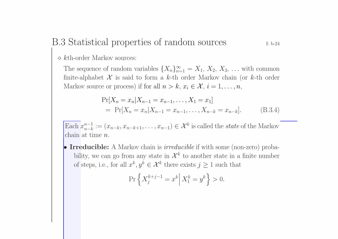
kth-order Markov sources:
The sequence of random variables Xn∞n=1 = X1, X2, X3, . . . with common
finite-alphabet X is said to form a k-th order Markov chain (or k-th order
Markov source or process) if for all n > k, xi ∈ X , i = 1, . . . , n,
Pr[Xn = xn|Xn−1 = xn−1, . . . , X1 = x1]
= Pr[Xn = xn|Xn−1 = xn−1, . . . , Xn−k = xn−k]. (B.3.4)
Each xn−1n−k := (xn−k, xn−k+1, . . . , xn−1) ∈ X k is called the state of the Markov
chain at time n.
• Irreducible: A Markov chain is irreducible if with some (non-zero) proba-
bility, we can go from any state in X k to another state in a finite number
of steps, i.e., for all xk, yk ∈ X k there exists j ≥ 1 such that
PrXk+j−1
j = xk∣∣∣Xk
1 = yk> 0.
B.3 Statistical properties of random sources I: b-25
• Time-invariant: A Markov chain is said to be time-invariant or homo-
geneous, if for every n > k,
Pr[Xn = xn|Xn−1 = xn−1, . . . , Xn−k = xn−k]
= Pr[Xk+1 = xk+1|Xk = xk, . . . , X1 = x1].
– Therefore, a homogeneous first-order Markov chain can be defined thr-
ough its transition probability:[PrX2 = x2|X1 = x1
]|X |×|X |,
and its initial state distribution PX1(x).
B.3 Statistical properties of random sources I: b-26
• Aperiodic:
– In a first-order Markov chain, the period d(x) of state x ∈ X is defined
by
d(x):=gcd n ∈ 1, 2, 3, . . . : PrXn+1 = x|X1 = x > 0 ,where gcd denotes the greatest common divisor; in other words, if the
Markov chain starts in state x, then the chain cannot return to state x
at any time that is not a multiple of d(x).
– If PrXn+1 = x|X1 = x = 0 for all n, we say that state x has an
infinite period and write d(x) = ∞.
– We also say that state x is aperiodic if d(x) = 1 and periodic if d(x) >
1.
– The first-order Markov chain is called aperiodic if all its states are
aperiodic. In other words, the first-order Markov chain is aperiodic if
gcd n ∈ 1, 2, 3, . . . : PrXn+1 = x|X1 = x > 0 = 1 ∀x ∈ X .
Property. In an irreducible first-order Markov chain, all states have the
same period. Hence, if one state in such a chain is aperiodic, then the entire
Markov chain is aperiodic.
B.3 Statistical properties of random sources I: b-27
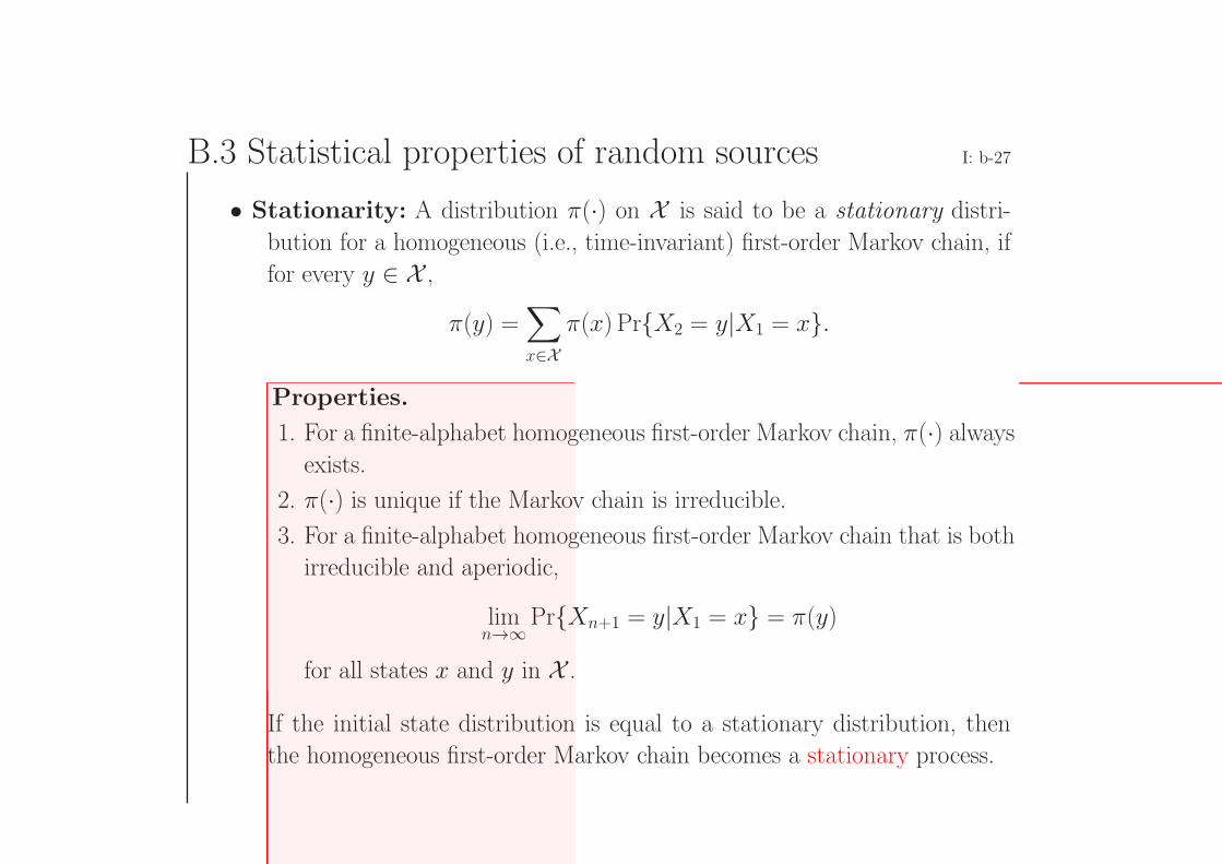
• Stationarity: A distribution π(·) on X is said to be a stationary distri-
bution for a homogeneous (i.e., time-invariant) first-order Markov chain, if
for every y ∈ X ,
π(y) =∑x∈X
π(x) PrX2 = y|X1 = x.
Properties.
1. For a finite-alphabet homogeneous first-order Markov chain, π(·) alwaysexists.
2. π(·) is unique if the Markov chain is irreducible.
3. For a finite-alphabet homogeneous first-order Markov chain that is both
irreducible and aperiodic,
limn→∞PrXn+1 = y|X1 = x = π(y)
for all states x and y in X .
If the initial state distribution is equal to a stationary distribution, then
the homogeneous first-order Markov chain becomes a stationary process.
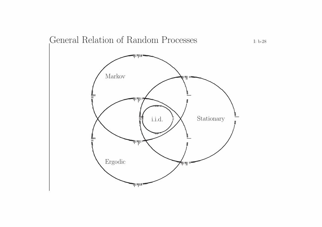
General Relation of Random Processes I: b-28
Markov
i.i.d. Stationary
Ergodic
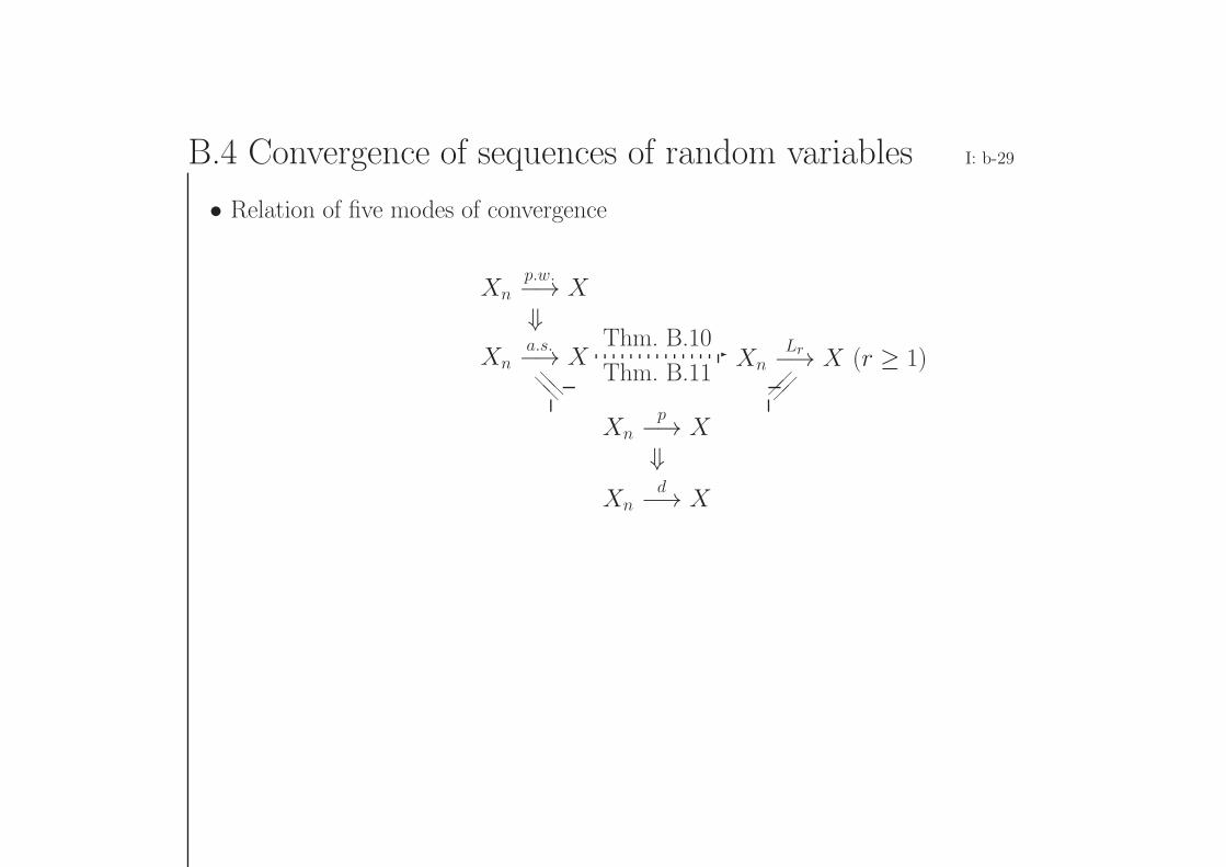
B.4 Convergence of sequences of random variables I: b-29
• Relation of five modes of convergence
Thm. B.10
Thm. B.11
Xnp.w.−→ X⇓
Xna.s.−→ X
XnLr−→ X (r ≥ 1)
Xnp−→ X⇓
Xnd−→ X
B.4 Convergence of sequences of random variables I: b-30
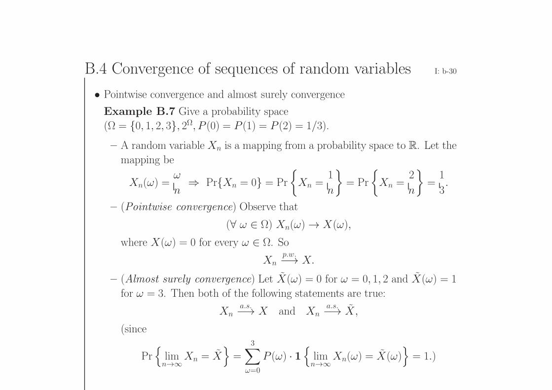
• Pointwise convergence and almost surely convergence
Example B.7 Give a probability space
(Ω = 0, 1, 2, 3, 2Ω, P (0) = P (1) = P (2) = 1/3).
– A random variable Xn is a mapping from a probability space to R. Let the
mapping be
Xn(ω) =ω
n⇒ PrXn = 0 = Pr
Xn =
1
n
= Pr
Xn =
2
n
=
1
3.
– (Pointwise convergence) Observe that
(∀ ω ∈ Ω) Xn(ω) → X(ω),
where X(ω) = 0 for every ω ∈ Ω. So
Xnp.w.−→ X.
– (Almost surely convergence) Let X(ω) = 0 for ω = 0, 1, 2 and X(ω) = 1
for ω = 3. Then both of the following statements are true:
Xna.s.−→ X and Xn
a.s.−→ X,
(since
Prlimn→∞Xn = X
=
3∑ω=0
P (ω) · 1limn→∞Xn(ω) = X(ω)
= 1.)
B.4 Convergence of sequences of random variables I: b-31
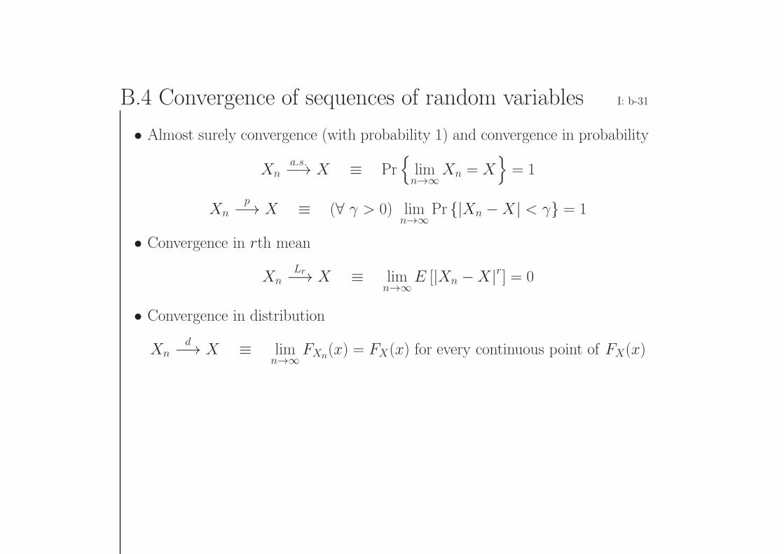
• Almost surely convergence (with probability 1) and convergence in probability
Xna.s.−→ X ≡ Pr
limn→∞Xn = X
= 1
Xnp−→ X ≡ (∀ γ > 0) lim
n→∞Pr |Xn −X| < γ = 1
• Convergence in rth mean
XnLr−→ X ≡ lim
n→∞E [|Xn −X|r] = 0
• Convergence in distribution
Xnd−→ X ≡ lim
n→∞FXn(x) = FX(x) for every continuous point of FX(x)
B.4 Convergence of sequences of random variables I: b-32
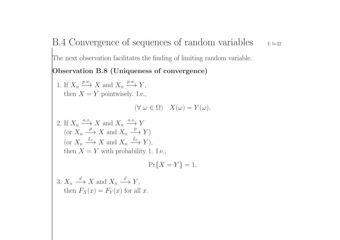
The next observation facilitates the finding of limiting random variable.
Observation B.8 (Uniqueness of convergence)
1. If Xnp.w.−→ X and Xn
p.w.−→ Y ,
then X = Y pointwisely. I.e.,
(∀ ω ∈ Ω) X(ω) = Y (ω).
2. If Xna.s.−→ X and Xn
a.s.−→ Y
(or Xnp−→ X and Xn
p−→ Y )
(or XnLr−→ X and Xn
Lr−→ Y ),
then X = Y with probability 1. I.e.,
PrX = Y = 1.
3. Xnd−→ X and Xn
d−→ Y ,
then FX(x) = FY (x) for all x.
B.4 Convergence of sequences of random variables I: b-33
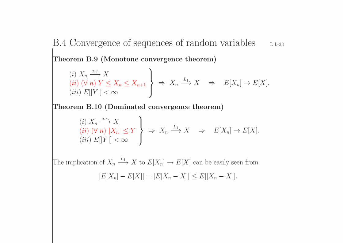
Theorem B.9 (Monotone convergence theorem)
(i) Xna.s.−→ X
(ii) (∀ n) Y ≤ Xn ≤ Xn+1
(iii) E[|Y |] < ∞
⇒ Xn
L1−→ X ⇒ E[Xn] → E[X ].
Theorem B.10 (Dominated convergence theorem)
(i) Xna.s.−→ X
(ii) (∀ n) |Xn| ≤ Y
(iii) E[|Y |] < ∞
⇒ Xn
L1−→ X ⇒ E[Xn] → E[X ].
The implication of XnL1−→ X to E[Xn] → E[X ] can be easily seen from
|E[Xn]− E[X ]| = |E[Xn −X ]| ≤ E[|Xn −X|].
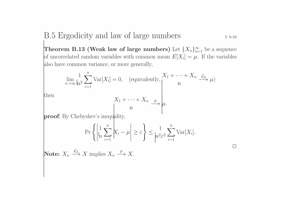
B.5 Ergodicity and law of large numbers I: b-34
Theorem B.13 (Weak law of large numbers) Let Xn∞n=1 be a sequence
of uncorrelated random variables with common mean E[Xi] = µ. If the variables
also have common variance, or more generally,
limn→∞
1
n2
n∑i=1
Var[Xi] = 0, (equivalently,X1 + · · · +Xn
n
L2−→ µ)
thenX1 + · · · +Xn
n
p−→ µ.
proof: By Chebyshev’s inequality,
Pr
∣∣∣∣∣1nn∑
i=1
Xi − µ
∣∣∣∣∣ ≥ ε
≤ 1
n2ε2
n∑i=1
Var[Xi].
Note: XnL2−→ X implies Xn
p−→ X .
B.5 Ergodicity and law of large numbers I: b-35
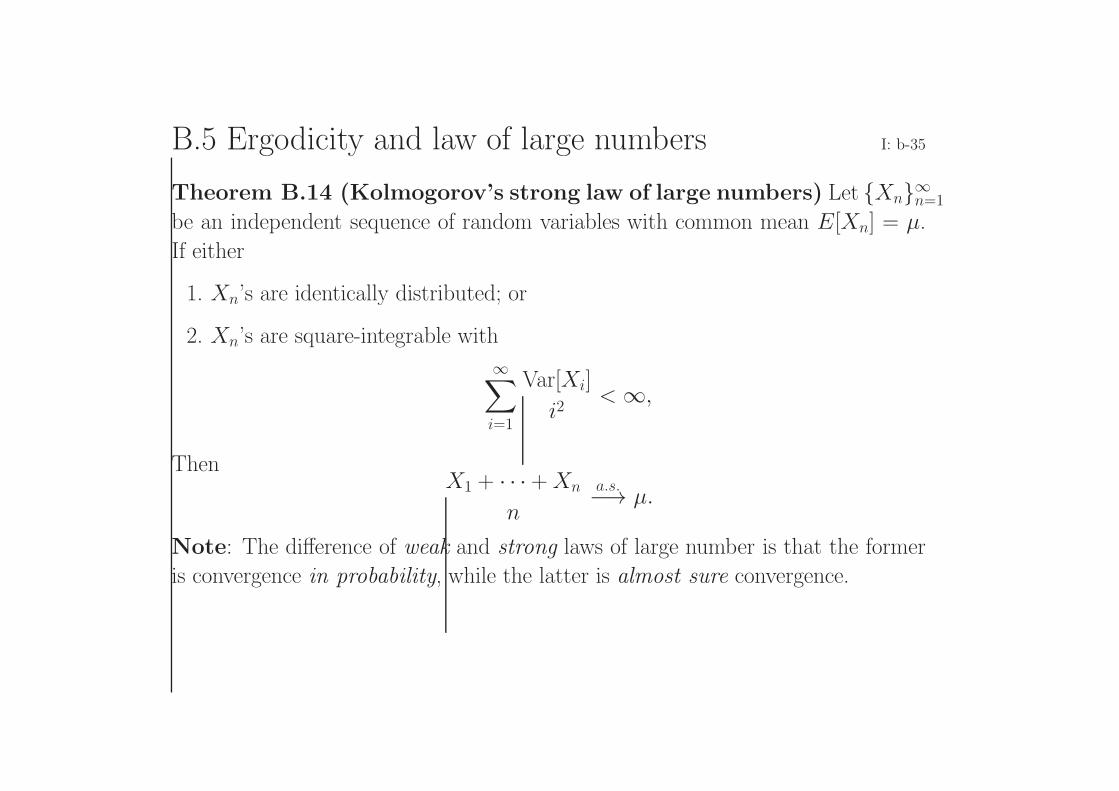
Theorem B.14 (Kolmogorov’s strong law of large numbers) Let Xn∞n=1
be an independent sequence of random variables with common mean E[Xn] = µ.
If either
1. Xn’s are identically distributed; or
2. Xn’s are square-integrable with
∞∑i=1
Var[Xi]
i2< ∞,
ThenX1 + · · · +Xn
n
a.s.−→ µ.
Note: The difference of weak and strong laws of large number is that the former
is convergence in probability, while the latter is almost sure convergence.
B.5 Ergodicity and law of large numbers I: b-36
• After the introduction of Kolmogorov’s strong law of large numbers, one may
find that the pointwise ergodic theorem (Theorem B.4) actually indicates a
similar result.
– In fact, the pointwise ergodic theorem can be viewed as another version of
strong law of large numbers, which states that for stationary and ergodic
processes, time averages converge with probability 1 to the ensemble
expectation.
• The notion of ergodicity is often misinterpreted, since the definition is not very
intuitive. Some engineering texts may provide a definition that a stationary
process satisfying the ergodic theorem is also ergodic.
B.5 Ergodicity and law of large numbers I: b-37
Let us try to clarify the notion of ergodicity by the following remarks.
• The concept of ergodicity does not require stationarity. In other words, a
non-stationary process can be ergodic.
• Many perfectly good models of physical processes are not ergodic, yet they
have a form of law of large numbers. In other words, non-ergodic processes can
be perfectly good and useful models.
• There is no finite-dimensional equivalent definition of ergodicity as there is
for stationarity. This fact makes it more difficult to describe and interpret
ergodicity.
• I.i.d. processes are ergodic; hence, ergodicity can be thought of as a (kind of)
generalization of i.i.d.
• As mentioned earlier, stationarity and ergodicity imply the time average con-
verges with probability 1 to the ensemble mean. Now if a process is stationary
but not ergodic, then the time average still converges, but possibly not to the
ensemble mean.
B.5 Ergodicity and law of large numbers I: b-38
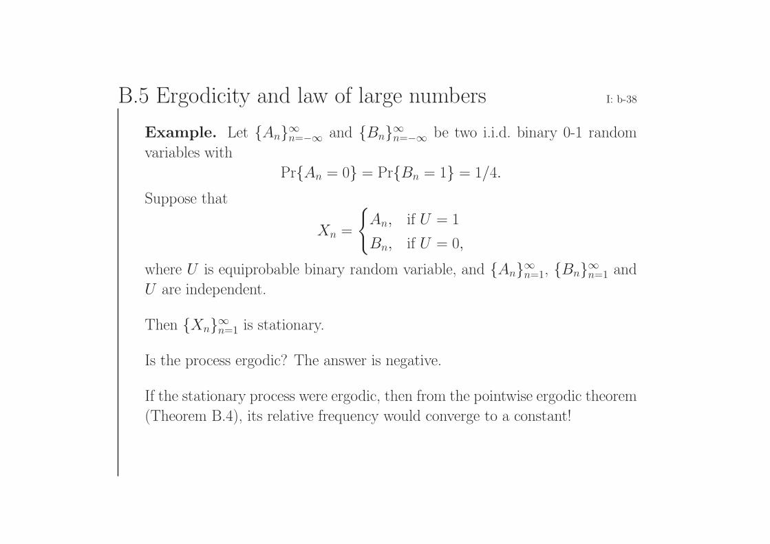
Example. Let An∞n=−∞ and Bn∞n=−∞ be two i.i.d. binary 0-1 random
variables with
PrAn = 0 = PrBn = 1 = 1/4.
Suppose that
Xn =
An, if U = 1
Bn, if U = 0,
where U is equiprobable binary random variable, and An∞n=1, Bn∞n=1 and
U are independent.
Then Xn∞n=1 is stationary.
Is the process ergodic? The answer is negative.
If the stationary process were ergodic, then from the pointwise ergodic theorem
(Theorem B.4), its relative frequency would converge to a constant!
B.5 Ergodicity and law of large numbers I: b-39
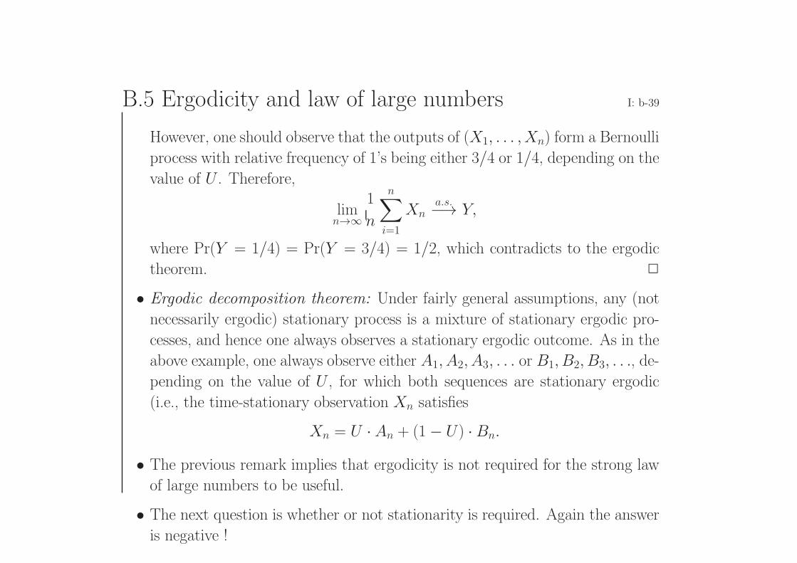
However, one should observe that the outputs of (X1, . . . , Xn) form a Bernoulli
process with relative frequency of 1’s being either 3/4 or 1/4, depending on the
value of U . Therefore,
limn→∞
1
n
n∑i=1
Xna.s.−→ Y,
where Pr(Y = 1/4) = Pr(Y = 3/4) = 1/2, which contradicts to the ergodic
theorem.
• Ergodic decomposition theorem: Under fairly general assumptions, any (not
necessarily ergodic) stationary process is a mixture of stationary ergodic pro-
cesses, and hence one always observes a stationary ergodic outcome. As in the
above example, one always observe either A1, A2, A3, . . . or B1, B2, B3, . . ., de-
pending on the value of U , for which both sequences are stationary ergodic
(i.e., the time-stationary observation Xn satisfies
Xn = U · An + (1− U) · Bn.
• The previous remark implies that ergodicity is not required for the strong law
of large numbers to be useful.
• The next question is whether or not stationarity is required. Again the answer
is negative !
B.5 Ergodicity and law of large numbers I: b-40
• In fact, what is needed in this course is the law of large numbers, which
results the convergence of sample averages to its ensemble expectation.
– It should be reasonable to expect that random processes could exhibit tran-
sient behavior that violates the stationarity definition, yet the sample av-
erage still converges. One can then introduce the notion of asymptotically
stationary to achieve the law of large numbers.

B.6 Central limit theorem I: b-41
Theorem B.15 (Central limit theorem) If Xn∞n=1 is a sequence of i.i.d. ran-
dom variables with finite common marginal mean µ and variance σ2, then
1√n
n∑i=1
(Xi − µ)d−→ Z ∼ N (0, σ2),
where the convergence is in distribution (as n → ∞) and Z ∼ N (0, σ2) is a
Gaussian distributed random variable with mean 0 and variance σ2.
B.7 Convexity, concavity and Jensen’s inequality I: b-42
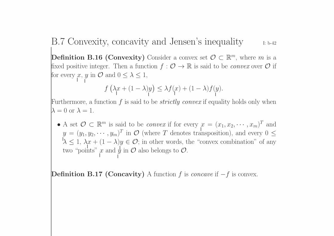
Definition B.16 (Convexity) Consider a convex set O ⊂ Rm, where m is a
fixed positive integer. Then a function f : O → R is said to be convex over O if
for every x, y in O and 0 ≤ λ ≤ 1,
f(λx + (1− λ)y
) ≤ λf(x) + (1− λ)f(y).
Furthermore, a function f is said to be strictly convex if equality holds only when
λ = 0 or λ = 1.
• A set O ⊂ Rm is said to be convex if for every x = (x1, x2, · · · , xm)T and
y = (y1, y2, · · · , ym)T in O (where T denotes transposition), and every 0 ≤λ ≤ 1, λx + (1 − λ)y ∈ O; in other words, the “convex combination” of any
two “points” x and y in O also belongs to O.
Definition B.17 (Concavity) A function f is concave if −f is convex.
Jensen’s inequality I: b-43
Theorem B.18 (Jensen’s inequality) If f : O → R is convex over a convex
set O ⊂ Rm, and X = (X1, X2, · · · , Xm)
T is an m-dimensional random vector
with alphabet X ⊂ O, then
E[f(X)] ≥ f(E[X ]).
Moreover, if f is strictly convex, then equality in the above inequality immediately
implies X = E[X ] with probability 1.
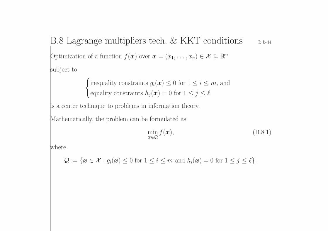
B.8 Lagrange multipliers tech. & KKT conditions I: b-44
Optimization of a function f(x) over x = (x1, . . . , xn) ∈ X ⊆ Rn
subject to inequality constraints gi(x) ≤ 0 for 1 ≤ i ≤ m, and
equality constraints hj(x) = 0 for 1 ≤ j ≤
is a center technique to problems in information theory.
Mathematically, the problem can be formulated as:
minx∈Q
f(x), (B.8.1)
where
Q := x ∈ X : gi(x) ≤ 0 for 1 ≤ i ≤ m and hi(x) = 0 for 1 ≤ j ≤ .
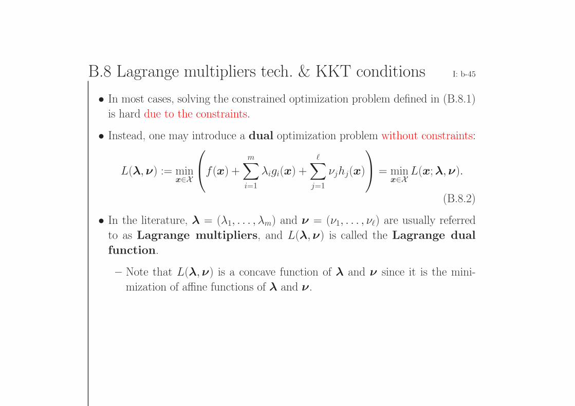
B.8 Lagrange multipliers tech. & KKT conditions I: b-45
• In most cases, solving the constrained optimization problem defined in (B.8.1)
is hard due to the constraints.
• Instead, one may introduce a dual optimization problem without constraints:
L(λ,ν) := minx∈X
f(x) + m∑
i=1
λigi(x) +
∑j=1
νjhj(x)
= min
x∈XL(x;λ,ν).
(B.8.2)
• In the literature, λ = (λ1, . . . , λm) and ν = (ν1, . . . , ν) are usually referred
to as Lagrange multipliers, and L(λ,ν) is called the Lagrange dual
function.
– Note that L(λ,ν) is a concave function of λ and ν since it is the mini-
mization of affine functions of λ and ν.
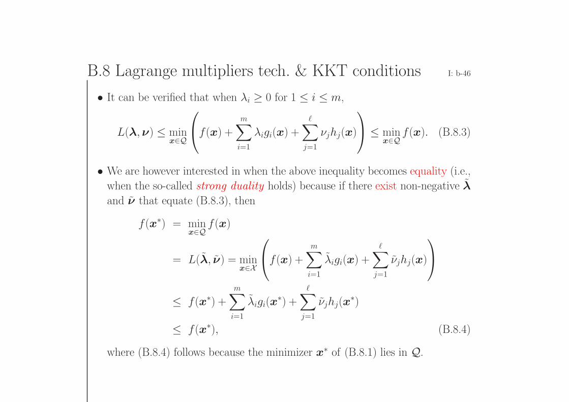
B.8 Lagrange multipliers tech. & KKT conditions I: b-46
• It can be verified that when λi ≥ 0 for 1 ≤ i ≤ m,
L(λ,ν) ≤ minx∈Q
f(x) + m∑
i=1
λigi(x) +∑
j=1
νjhj(x)
≤ min
x∈Qf(x). (B.8.3)
• We are however interested in when the above inequality becomes equality (i.e.,
when the so-called strong duality holds) because if there exist non-negative λ
and ν that equate (B.8.3), then
f(x∗) = minx∈Q
f(x)
= L(λ, ν) = minx∈X
f(x) + m∑
i=1
λigi(x) +
∑j=1
νjhj(x)
≤ f(x∗) +m∑i=1
λigi(x∗) +
∑j=1
νjhj(x∗)
≤ f(x∗), (B.8.4)
where (B.8.4) follows because the minimizer x∗ of (B.8.1) lies in Q.
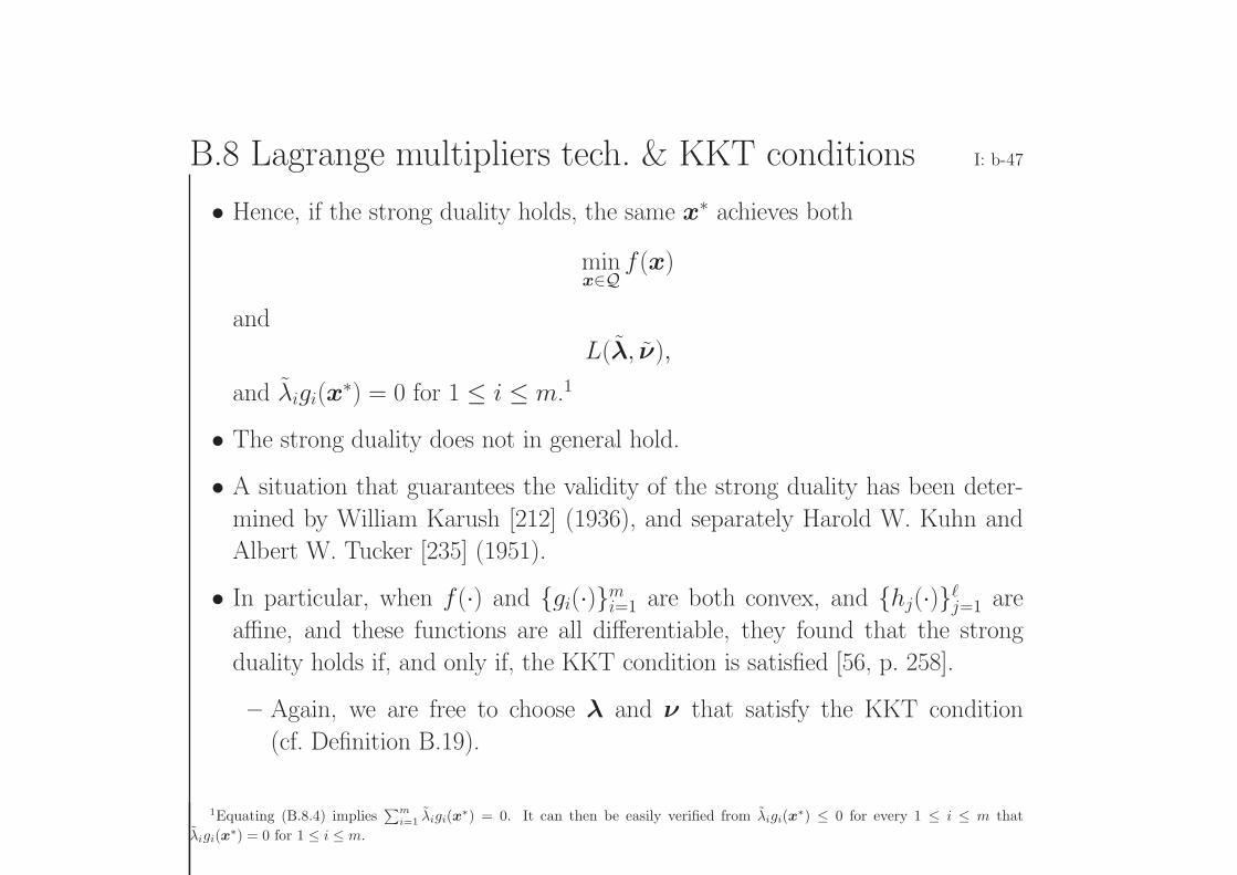
B.8 Lagrange multipliers tech. & KKT conditions I: b-47
• Hence, if the strong duality holds, the same x∗ achieves both
minx∈Q
f(x)
and
L(λ, ν),
and λigi(x∗) = 0 for 1 ≤ i ≤ m.1
• The strong duality does not in general hold.
• A situation that guarantees the validity of the strong duality has been deter-
mined by William Karush [212] (1936), and separately Harold W. Kuhn and
Albert W. Tucker [235] (1951).
• In particular, when f(·) and gi(·)mi=1 are both convex, and hj(·)j=1 are
affine, and these functions are all differentiable, they found that the strong
duality holds if, and only if, the KKT condition is satisfied [56, p. 258].
– Again, we are free to choose λ and ν that satisfy the KKT condition
(cf. Definition B.19).
1Equating (B.8.4) implies∑m
i=1 λigi(x∗) = 0. It can then be easily verified from λigi(x
∗) ≤ 0 for every 1 ≤ i ≤ m that
λigi(x∗) = 0 for 1 ≤ i ≤ m.
B.8 Lagrange multipliers tech. & KKT conditions I: b-48
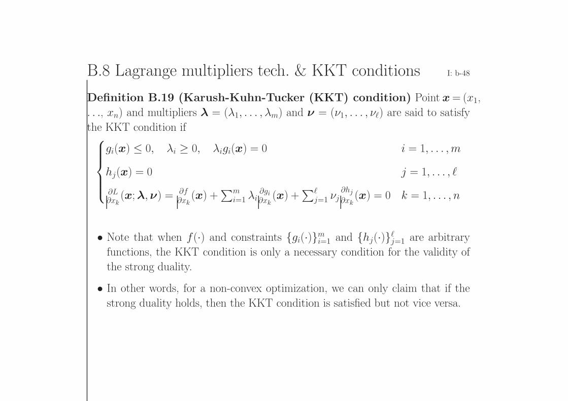
Definition B.19 (Karush-Kuhn-Tucker (KKT) condition) Point x= (x1,
. . ., xn) and multipliers λ = (λ1, . . . , λm) and ν = (ν1, . . . , ν) are said to satisfy
the KKT condition ifgi(x) ≤ 0, λi ≥ 0, λigi(x) = 0 i = 1, . . . ,m
hj(x) = 0 j = 1, . . . ,
∂L∂xk
(x;λ,ν) = ∂f∂xk
(x) +∑m
i=1 λi∂gi∂xk
(x) +∑
j=1 νj∂hj∂xk
(x) = 0 k = 1, . . . , n
• Note that when f(·) and constraints gi(·)mi=1 and hj(·)j=1 are arbitrary
functions, the KKT condition is only a necessary condition for the validity of
the strong duality.
• In other words, for a non-convex optimization, we can only claim that if the
strong duality holds, then the KKT condition is satisfied but not vice versa.
B.8 Lagrange multipliers tech. & KKT conditions I: b-49
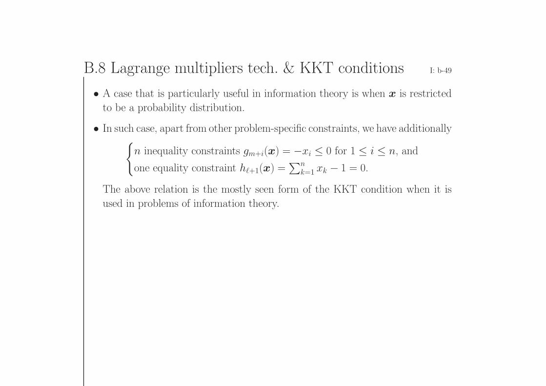
• A case that is particularly useful in information theory is when x is restricted
to be a probability distribution.
• In such case, apart from other problem-specific constraints, we have additionallyn inequality constraints gm+i(x) = −xi ≤ 0 for 1 ≤ i ≤ n, and
one equality constraint h+1(x) =∑n
k=1 xk − 1 = 0.
The above relation is the mostly seen form of the KKT condition when it is
used in problems of information theory.
B.8 Lagrange multipliers tech. & KKT conditions I: b-50
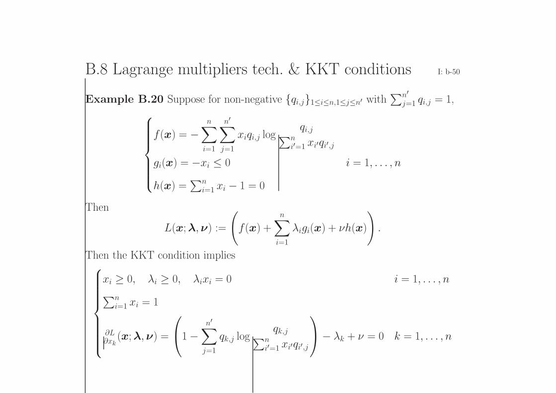
Example B.20 Suppose for non-negative qi,j1≤i≤n,1≤j≤n′ with∑n′
j=1 qi,j = 1,f(x) = −
n∑i=1
n′∑j=1
xiqi,j logqi,j∑n
i′=1 xi′qi′,j
gi(x) = −xi ≤ 0 i = 1, . . . , n
h(x) =∑n
i=1 xi − 1 = 0
Then
L(x;λ,ν) :=
(f(x) +
n∑i=1
λigi(x) + νh(x)
).
Then the KKT condition implies
xi ≥ 0, λi ≥ 0, λixi = 0 i = 1, . . . , n∑ni=1 xi = 1
∂L∂xk
(x;λ,ν) =
1− n′∑
j=1
qk,j logqk,j∑n
i′=1 xi′qi′,j
− λk + ν = 0 k = 1, . . . , n
B.8 Lagrange multipliers tech. & KKT conditions I: b-51
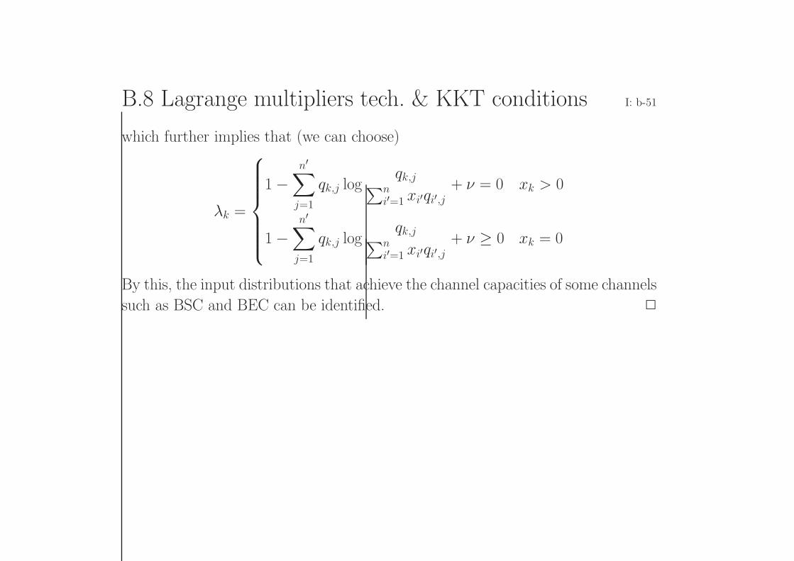
which further implies that (we can choose)
λk =
1−
n′∑j=1
qk,j logqk,j∑n
i′=1 xi′qi′,j+ ν = 0 xk > 0
1−n′∑j=1
qk,j logqk,j∑n
i′=1 xi′qi′,j+ ν ≥ 0 xk = 0
By this, the input distributions that achieve the channel capacities of some channels
such as BSC and BEC can be identified.
Key Notes I: b-52
• Definitions of (weakly, strictly) stationarity, ergodicity and Markovian (irre-
ducible, homogeneous)
• Mode of convergences (almost surely or with probability 1, in probability, in
distribution, in Lr mean)
• Laws of large numbers
• Central limit theorem
• Jensen’s inequality (convexity and concavity)
• KKT conditions