Appendix A Fundamentals of Heat Transfer - Springer978-3-662-46379-6/1.pdfAppendix A Fundamentals of...

Appendix AFundamentals of Heat Transfer

A.1 Heat Conduction

When a temperature gradient exists in a body, energy will transfer from the high-temperature region to the low-temperature region by conduction. The general equa-tions of heat conduction is given by [1]

∇ · (k∇T) + q̇in = ρc∂T

∂t(A.1)

where T is temperature; q̇in is energy generated per unit volume; k, ρ, and c arethermal conductivity, density and specific heat, respectively.

In fire engineering, one-dimensional (1D) heat transfer is usually considered. Theequation of 1D conduction is given by (ignore energy generation, thus q̇in = 0)

∂2T

∂x2= 1

α

∂T

∂t(A.2)

where α = k�ρc is thermal diffusivity.Fourier’s law states that the quantity of heat transferred per unit time per unit area isproportional to the temperature gradient, thus

q̇ = −k∂T

∂x(A.3)

To solve Eq.A.2, the following boundary conditions are usually used [2, 3]

1. Initial condition,T(x, 0) = T∞ (A.4)

2. Dirichlet condition,T(0, t) = Tg(t) (A.5)

© Springer-Verlag Berlin Heidelberg 2015C. Zhang, Reliability of Steel Columns Protected by Intumescent CoatingsSubjected to Natural Fires, Springer Theses, DOI 10.1007/978-3-662-46379-6

113

114 Appendix A: Fundamentals of Heat Transfer

3. Neumann condition,

− k∂T

∂x(0, t) = q̇0 = h[Tg(t) − T(0, t)] (A.6)

where, x denotes opposite normal direction to the surface; T∞, Tg are environmenttemperature and fire temperature, respectively; q̇0 is heat flux per unit time transferredfrom fire environment to the surface; and h is coefficient for convection or radiation.

In unsteady or transient conduction, Boit number is used to determine whether abody can be treated as thermally thin or thermally thick, which is defined by [1]

Bi = δ/k

1/h= hδ

k(A.7)

where, δ = V/A is the characteristic length of the body, in which V and A are thebody’s solid volume and its surface area.

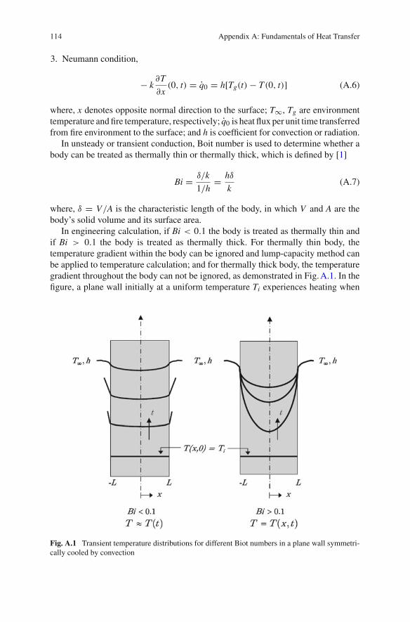
In engineering calculation, if Bi < 0.1 the body is treated as thermally thin andif Bi > 0.1 the body is treated as thermally thick. For thermally thin body, thetemperature gradient within the body can be ignored and lump-capacity method canbe applied to temperature calculation; and for thermally thick body, the temperaturegradient throughout the body can not be ignored, as demonstrated in Fig.A.1. In thefigure, a plane wall initially at a uniform temperature Ti experiences heating when

Fig. A.1 Transient temperature distributions for different Biot numbers in a plane wall symmetri-cally cooled by convection

Appendix A: Fundamentals of Heat Transfer 115

immersed in a fluid of T∞ < Ti. The problem can be treated as one dimensionalin x and the temperature variation with position and time, T(x, t) is shown. Thetemperature variation throughout the section is seen to a strong function of the Biotnumber. When the Biot number is small, temperature gradients in the solid are smalland the main temperature difference is between the solid and the fluid, and the solidtemperature remains nearly uniform as it increases to T∞. For large values of the Biotnumber, temperature gradients within the solid can be significant and the temperaturedifference across the solid is much larger than that between the surface and the fluid.

The temperature of a thermally thin body (Bi < 0.1) under a initial boundarygiven by Eq.A.4 and a Neumann boundary given by Eq.A.6 (A example of this caseis a bare steel member fully engulfed by fire), calculated by using lumped-capacitymethod, is given by [1]

T − T∞Tg − T∞

= exp

(− hA

ρcVt

)= e−Bi·Fo (A.8)

whereFo = αt/δ2 is Fourier number. TakeFo = 1,we can get the thermal penetrationtime of the thermal thin body, given by [4]

tpthin = δ2

α. (A.9)

The thermal penetration time is the time required for a thermal pulse to reach theback face of the body [5].

For thermally thick bodies (Bi > 0.1) like concrete walls and concrete slabs, infire engineering calculations the bodies are usually treated as semi-infinite bodies.The temperature of a semi-infinity solid under a initial boundary given by Eq.A.4and a Neumann boundary given by Eq.A.6 is give by [2, 3]

T − T∞Tg − T∞

= erfc

(x

2√

αt

)− exp

(xh

k+ αt

(k/h)2

)· erfc

(x

2√

αt+

√αt

k/h

)(A.10)

where, erfc(ξ) = 1 − erf (ξ). erf (ξ) is the error function, given by

erf (ξ) = 2

π

∫ ξ

0e−η2dη (A.11)

Take αt�(k/h)2 = 1 or√

αt/(k/h) = 1, we get the thermal penetration time ofthe thermally thick body, given by [4]:

tpthick = (k/h)2

α= kρc

h2(A.12)

The temperature of the same semi-infinity body under a initial boundary given byEq.A.4 and a Dirichlet boundary given by Eq.A.5 is given by


T − T∞Tg − T∞

= 1 − erf

(x

2√

αt

)(A.13)

Take Eq.A.13=0.005, we get

x = L ≈ 4√

αt (A.14)

where L is the distance to the surface at which the temperature decreases to 0.5% ofthe surface temperature. EquationA.14 indicated that a wall or slab, can be treatedas a semi-infinite solid with little error, provided its thickness is greater than 4

√αt.

In fire engineering, if the thickness of a wall or slab is greater than 2√

αt, the semi-infinite solid assumption is used and the corresponding thermal penetration time isgiven by [2, 5]

tp = 1

α

(δw

2

)2

(A.15)

where δw is the thickness of the wall or slab.

A.2 Heat Convection

Convection describes the energy transfer between a surface and a fluid moving overthat surface as a result of an imposed temperature difference. Strictly, convection isnot a basic model of heat transfer, rather it can be considered as a combined effect ofconduction and themotion of some transmittingmedium (The only two basic modelsof heat transfer are conduction and radiation). In general, however, convection istreated as a separate mode of heat transfer involving complex relationships betweenvelocity, temperature and concentration distributions.

Newton’s law of cooling states that the heat flux transferred by convection, q̇c, isproportional to the difference in temperature between the surface and the fluid, that

q̇c = hc(T∞ − Ts) (A.16)

where the proportionality constant hc is the convection heat transfer coefficient orfilm coefficient; Ts is surface temperature; and T∞ is the fluid temperature far awayfrom the surface.

By the boundary layer concept, the heat flux transferred from fluid to surface canalso be calculated by Fourier’s law in conduction, that [6]

q̇ = −kf∂T

∂y

∣∣∣∣y=0

≈ kf

δθ

(T∞ − Ts). (A.17)


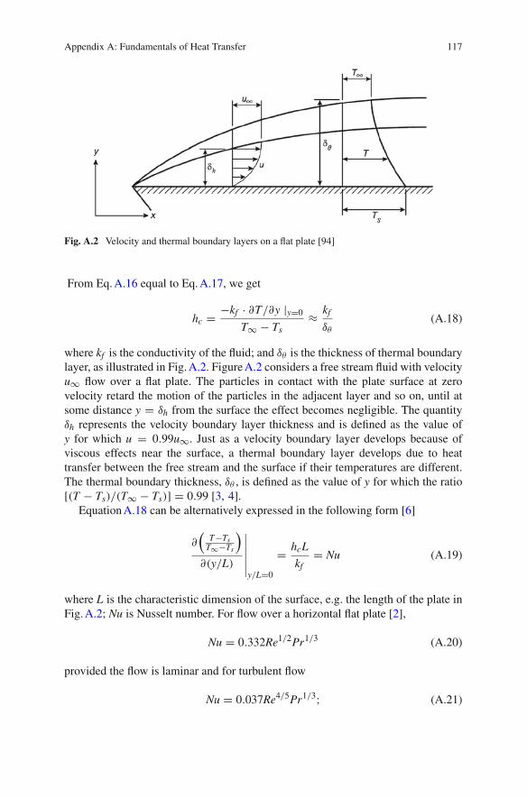
Fig. A.2 Velocity and thermal boundary layers on a flat plate [94]

From Eq.A.16 equal to Eq.A.17, we get

hc = −kf · ∂T/∂y |y=0

T∞ − Ts≈ kf

δθ

(A.18)

where kf is the conductivity of the fluid; and δθ is the thickness of thermal boundarylayer, as illustrated in Fig.A.2. FigureA.2 considers a free stream fluid with velocityu∞ flow over a flat plate. The particles in contact with the plate surface at zerovelocity retard the motion of the particles in the adjacent layer and so on, until atsome distance y = δh from the surface the effect becomes negligible. The quantityδh represents the velocity boundary layer thickness and is defined as the value ofy for which u = 0.99u∞. Just as a velocity boundary layer develops because ofviscous effects near the surface, a thermal boundary layer develops due to heattransfer between the free stream and the surface if their temperatures are different.The thermal boundary thickness, δθ , is defined as the value of y for which the ratio[(T − Ts)/(T∞ − Ts)] = 0.99 [3, 4].

EquationA.18 can be alternatively expressed in the following form [6]

∂(

T−TsT∞−Ts

)∂(y/L)

∣∣∣∣∣∣y/L=0

= hcL

kf= Nu (A.19)

where L is the characteristic dimension of the surface, e.g. the length of the plate inFig.A.2; Nu is Nusselt number. For flow over a horizontal flat plate [2],

Nu = 0.332Re1/2Pr1/3 (A.20)

provided the flow is laminar and for turbulent flow

Nu = 0.037Re4/5Pr1/3; (A.21)


and for buoyancy flow over a vertical flat plate

Nu = 0.59(Gr · Pr)1/4 (A.22)

Nu = 0.59(Gr · Pr)1/4 (A.23)

provided that the flow is laminar; and for turbulent flow

Nu = 0.13(Gr · Pr)1/3 (A.24)

where Re = ρu∞L/μ, Pr = ν/α = μ/ρα and Gr = gβ(T∞ − Ts)L3/ν2 areReynold number, Prandtl number and Grashof number, respectively. ρ, u∞ and μ

are density, velocity and dynamic viscosity of the fluid, respectively and β is thereciprocal of 273 K.

In natural or free convection, the flow is created by buoyancy induced by thetemperature difference between the boundary layer and the ambient fluid (In forcedconvection, the fluid is flowing as a continuous stream past the surface), and for avertical flat plate,

Nu = 0.59(Gr · Pr)1/4 (A.25)

provided that the flow is laminar; and for turbulent flow

Nu = 0.13(Gr · Pr)1/3 (A.26)

where Re = ρu∞L/μ, Pr = ν/α = μ/ρα and Gr = gβ(T∞ − Ts)L3/ν2 areReynold number, Prandtl number and Grashof number, respectively. ρ, u∞ and μ

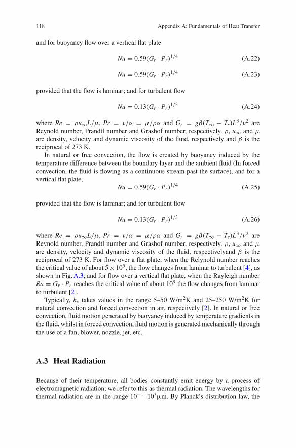
are density, velocity and dynamic viscosity of the fluid, respectivelyand β is thereciprocal of 273 K. For flow over a flat plate, when the Relynold number reachesthe critical value of about 5× 105, the flow changes from laminar to turbulent [4], asshown in Fig.A.3; and for flow over a vertical flat plate, when the Rayleigh numberRa = Gr · Pr reaches the critical value of about 109 the flow changes from laminarto turbulent [2].

Typically, hc takes values in the range 5–50 W/m2K and 25–250 W/m2K fornatural convection and forced convection in air, respectively [2]. In natural or freeconvection, fluid motion generated by buoyancy induced by temperature gradients inthe fluid, whilst in forced convection, fluidmotion is generatedmechanically throughthe use of a fan, blower, nozzle, jet, etc..

A.3 Heat Radiation

Because of their temperature, all bodies constantly emit energy by a process ofelectromagnetic radiation; we refer to this as thermal radiation. The wavelengths forthermal radiation are in the range 10−1–103µm. By Planck’s distribution law, the


Fig. A.3 Velocity boundary layer development on aflat plate showing laminar and turbulent regions,Rexc ≈ 5 × 105 [95]

spectral (or monochromatic) intensity of blackbody radiation is given by

Eb,λ = 2πc2hλ−5

exp(ch�kT) − 1(A.27)

where c is the velocity of light; h is Planck’s constant; k is Boltzmann’s constant;and T is the absolute temperature. The total emissive power of a black body is

Eb =∫ ∞

0Eb,λdλ = σT4 (A.28)

where σ = 5.67 × 10−8 W�m2K4 is Stefan-Boltzmann constant.A blackbody is defined as an ideal body that allows all the incident radiation to

pass into it (no reflected energy) and internally absorbs all the incident radiation (notransmitted energy) [7]. Other types of surfaces do not radiate as much energy as theblackbody. The total energy emitted by a real surface is

E = ε(Ts)Eb(Ts) = ε(Ts)σTs4 (A.29)

where ε(Ts) is emissivity of the surface, which is dependent on temperature. In prac-tice, constant values of emissivity for building materials are used. e.g. the emissivityof concrete and structural steel are taken as 0.7 in EC4 [8].


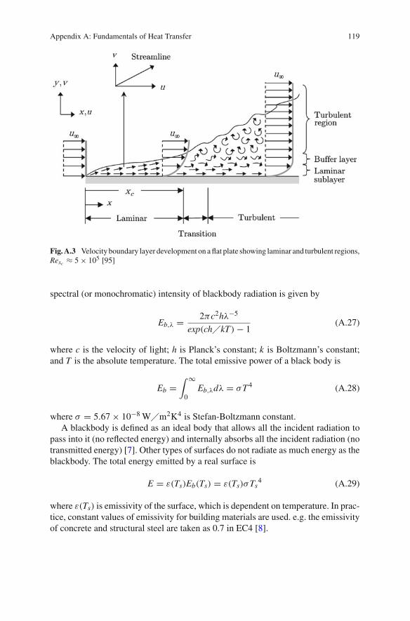
Fig. A.4 Absorption, reflection and transmission processes associated with a semitransparentmedium [95]

As shown in Fig.A.4, when a spectral component of radiation strikes a mediumsurface, portions of this radiation may be reflected, absorbed and transmitted. Byenergy balance,

ρλ + αλ + τλ = 1 (A.30)

where ρλ, αλ, and τλ denotes the fraction of energy absorbed by, reflected at, andtransmitted through the surface, or are reflectivity, absorptivity and transmissivity,respectively.

Kirchoff’s law states that in order to maintain equilibrium, absorptivity and emis-sivity must be related by

αλ = ελ (A.31)

A surface whose emittance is the same for all directions is called a diffuse emitter [9].If the spectral emittance is the same for all wavelength, thus ε = ελ, the surface isgray [9].

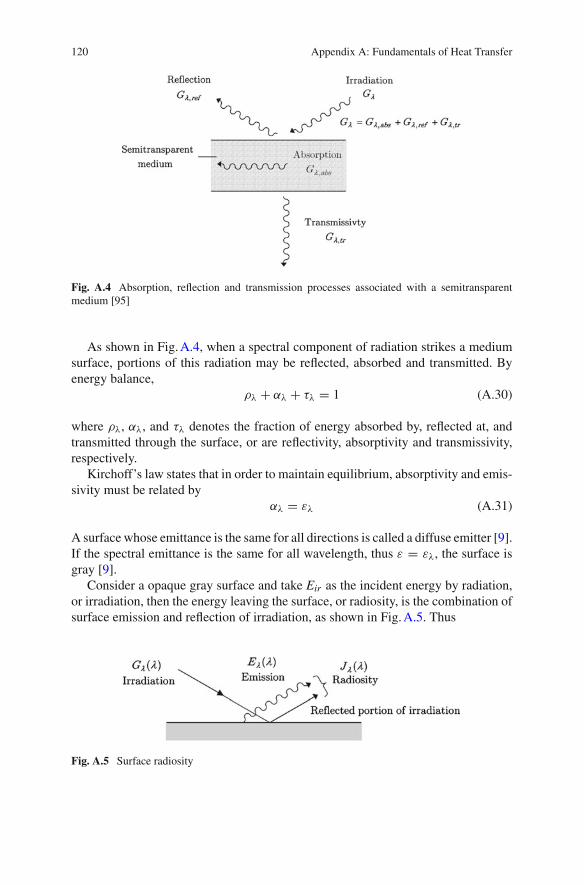
Consider a opaque gray surface and take Eir as the incident energy by radiation,or irradiation, then the energy leaving the surface, or radiosity, is the combination ofsurface emission and reflection of irradiation, as shown in Fig.A.5. Thus

Fig. A.5 Surface radiosity


Etot = ρEir + εEb = (1 − α)Eir + εEb = (1 − ε)Eir + εEb (A.32)

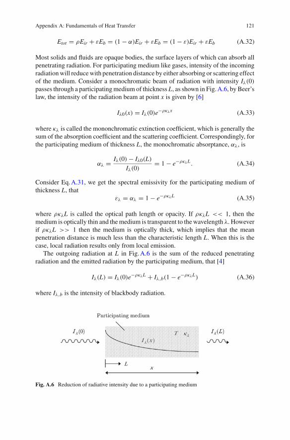
Most solids and fluids are opaque bodies, the surface layers of which can absorb allpenetrating radiation. For participating medium like gases, intensity of the incomingradiationwill reducewith penetration distance by either absorbing or scattering effectof the medium. Consider a monochromatic beam of radiation with intensity Iλ(0)passes through a participatingmedium of thickness L, as shown in Fig.A.6, by Beer’slaw, the intensity of the radiation beam at point x is given by [6]

Iλ0(x) = Iλ(0)e−ρκλx (A.33)

where κλ is called the mononchromatic extinction coefficient, which is generally thesum of the absorption coefficient and the scattering coefficient. Correspondingly, forthe participating medium of thickness L, the monochromatic absorptance, αλ, is

αλ = Iλ(0) − Iλ0(L)

Iλ(0)= 1 − e−ρκλL. (A.34)

Consider Eq.A.31, we get the spectral emissivity for the participating medium ofthickness L, that

ελ = αλ = 1 − e−ρκλL (A.35)

where ρκλL is called the optical path length or opacity. If ρκλL << 1, then themedium is optically thin and themedium is transparent to the wavelength λ. Howeverif ρκλL >> 1 then the medium is optically thick, which implies that the meanpenetration distance is much less than the characteristic length L. When this is thecase, local radiation results only from local emission.

The outgoing radiation at L in Fig.A.6 is the sum of the reduced penetratingradiation and the emitted radiation by the participating medium, that [4]

Iλ(L) = Iλ(0)e−ρκλL + Iλ,b(1 − e−ρκλL) (A.36)

where Iλ,b is the intensity of blackbody radiation.

Fig. A.6 Reduction of radiative intensity due to a participating medium


Monatomic and symmetric diatonic molecules such as N2 and O2 and H2 arecompletely transparent to thermal radiation, while asymmetrical molecules like CO2,H2O, CO, and SO2 absorb (and emit) thermal radiation of certain wavelengths [6].As a result, the absorptivity (or emissivity) of a air volume is mainly determined bythe volume fraction of H2O and CO2.

Combustion products include gases and soot. Soot particles are produced as aresult of incomplete combustion and are usually observed to be in the formof spheres,agglometrated chunks and long chains. The total emissivity of gas-soot mixture canbe calculated approximately by [4]

ε = (1 − e−κmL) + εge−κmL (A.37)

where κm is the mean absorption coefficient of the mixture, related to parameterslike soot volume fraction and temperature [9]

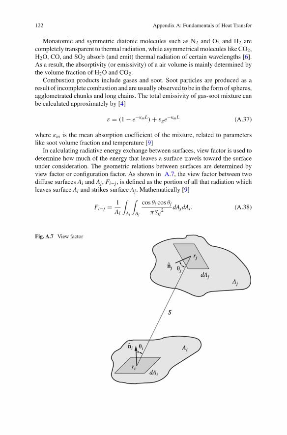
In calculating radiative energy exchange between surfaces, view factor is used todetermine how much of the energy that leaves a surface travels toward the surfaceunder consideration. The geometric relations between surfaces are determined byview factor or configuration factor. As shown in A.7, the view factor between twodiffuse surfaces Ai and Aj, Fi−j, is defined as the portion of all that radiation whichleaves surface Ai and strikes surface Aj. Mathematically [9]

Fi−j = 1

Ai

∫Ai

∫Aj

cos θi cos θj

πSij2 dAjdAi. (A.38)

Fig. A.7 View factor


Obviously,AiFi−j = AjFj−i (A.39)

N∑j=1

Fi−j = 1. (A.40)

Catalog of common view factors can be found in heat transfer handbooks suchas [6, 9].

Appendix BHigh Temperature Material Propertiesof Structural Steel

B.1 Thermal Properties

B.1.1 Coefficient of Thermal Elongation

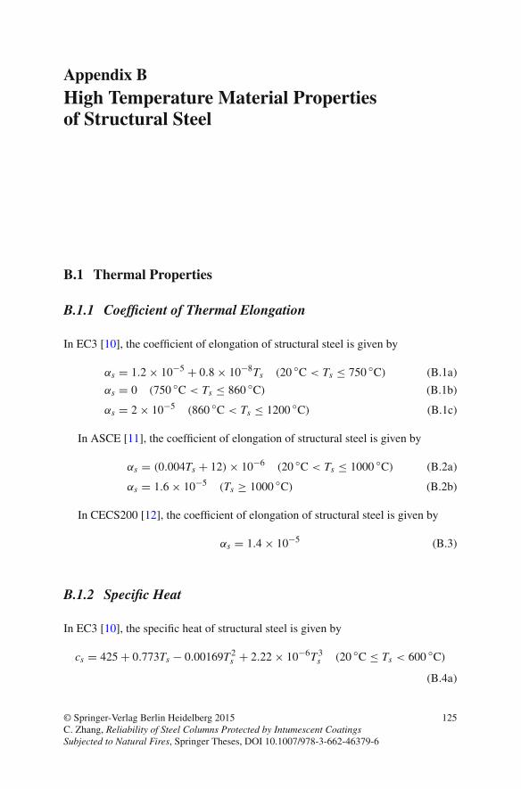
In EC3 [10], the coefficient of elongation of structural steel is given by

αs = 1.2 × 10−5 + 0.8 × 10−8Ts (20 ◦C < Ts ≤ 750 ◦C) (B.1a)

αs = 0 (750 ◦C < Ts ≤ 860 ◦C) (B.1b)

αs = 2 × 10−5 (860 ◦C < Ts ≤ 1200 ◦C) (B.1c)

In ASCE [11], the coefficient of elongation of structural steel is given by

αs = (0.004Ts + 12) × 10−6 (20 ◦C < Ts ≤ 1000 ◦C) (B.2a)

αs = 1.6 × 10−5 (Ts ≥ 1000 ◦C) (B.2b)

In CECS200 [12], the coefficient of elongation of structural steel is given by

αs = 1.4 × 10−5 (B.3)

B.1.2 Specific Heat

In EC3 [10], the specific heat of structural steel is given by

cs = 425 + 0.773Ts − 0.00169T2s + 2.22 × 10−6T3

s (20 ◦C ≤ Ts < 600 ◦C)

(B.4a)


125

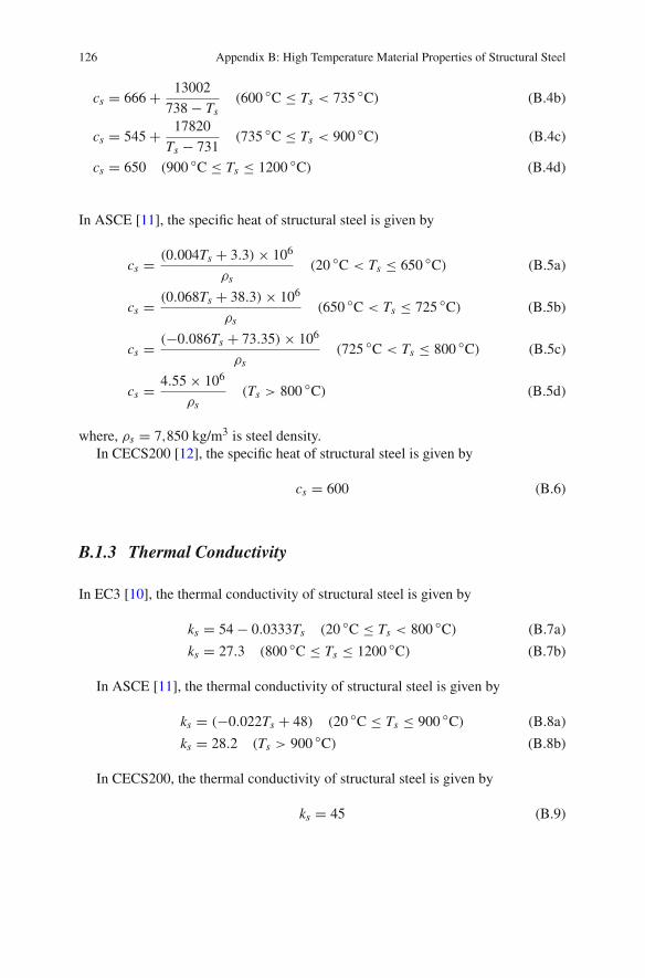
126 Appendix B: High Temperature Material Properties of Structural Steel

cs = 666 + 13002

738 − Ts(600 ◦C ≤ Ts < 735 ◦C) (B.4b)

cs = 545 + 17820

Ts − 731(735 ◦C ≤ Ts < 900 ◦C) (B.4c)

cs = 650 (900 ◦C ≤ Ts ≤ 1200 ◦C) (B.4d)

In ASCE [11], the specific heat of structural steel is given by

cs = (0.004Ts + 3.3) × 106

ρs(20 ◦C < Ts ≤ 650 ◦C) (B.5a)

cs = (0.068Ts + 38.3) × 106

ρs(650 ◦C < Ts ≤ 725 ◦C) (B.5b)

cs = (−0.086Ts + 73.35) × 106

ρs(725 ◦C < Ts ≤ 800 ◦C) (B.5c)

cs = 4.55 × 106

ρs(Ts > 800 ◦C) (B.5d)

where, ρs = 7,850 kg/m3 is steel density.In CECS200 [12], the specific heat of structural steel is given by

cs = 600 (B.6)

B.1.3 Thermal Conductivity

In EC3 [10], the thermal conductivity of structural steel is given by

ks = 54 − 0.0333Ts (20 ◦C ≤ Ts < 800 ◦C) (B.7a)

ks = 27.3 (800 ◦C ≤ Ts ≤ 1200 ◦C) (B.7b)

In ASCE [11], the thermal conductivity of structural steel is given by

ks = (−0.022Ts + 48) (20 ◦C ≤ Ts ≤ 900 ◦C) (B.8a)

ks = 28.2 (Ts > 900 ◦C) (B.8b)

In CECS200, the thermal conductivity of structural steel is given by

ks = 45 (B.9)

Appendix B: High Temperature Material Properties of Structural Steel 127

B.2 Structural Properties

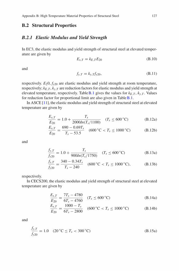
B.2.1 Elastic Modulus and Yield Strength

In EC3, the elastic modulus and yield strength of structural steel at elevated temper-ature are given by

Es,T = kE,T E20 (B.10)

andfy,T = ky,T fy20, (B.11)

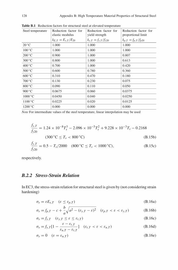
respectively. E20, fy20 are elastic modulus and yield strength at room temperature,respectively; kE,T , ky,T are reduction factors for elastic modulus and yield strength atelevated temperature, respectively. TableB.1 gives the values for kE,T , ky,T . Valuesfor reduction factor for proportional limit are also given in TableB.1.

In ASCE [11], the elastic modulus and yield strength of structural steel at elevatedtemperature are given by

Es,T

E20= 1.0 + Ts

2000In(Ts/1100)(Ts ≤ 600 ◦C) (B.12a)

Es,T

E20= 690 − 0.69Ts

Ts − 53.5(600 ◦C < Ts ≤ 1000 ◦C) (B.12b)

and

fy,Tfy20

= 1.0 + Ts

900In(Ts/1750)(Ts ≤ 600 ◦C) (B.13a)

fy,Tfy20

= 340 − 0.34Ts

Ts − 240(600 ◦C < Ts ≤ 1000 ◦C), (B.13b)

respectively.In CECS200, the elastic modulus and yield strength of structural steel at elevated

temperature are given by

Es,T

E20= 7Ts − 4780

6Ts − 4760(Ts ≤ 600 ◦C) (B.14a)

Es,T

E20= 1000 − Ts

6Ts − 2800(600 ◦C < Ts ≤ 1000 ◦C) (B.14b)

and

fy,Tfy20

= 1.0 (20 ◦C ≤ Ts < 300 ◦C) (B.15a)

128 Appendix B: High Temperature Material Properties of Structural Steel

Table B.1 Reduction factors for structural steel at elevated temperature

Steel temperature Reduction factor forelastic modulus

Reduction factor foryield strength

Reduction factor forproportional limit

kE,T = Es,T /E20 ky,T = fy,T /fy20 kp,T = fp,T /fp20

20 ◦C 1.000 1.000 1.000

100 ◦C 1.000 1.000 1.000

200 ◦C 0.900 1.000 0.807

300 ◦C 0.800 1.000 0.613

400 ◦C 0.700 1.000 0.420

500 ◦C 0.600 0.780 0.360

600 ◦C 0.310 0.470 0.180

700 ◦C 0.130 0.230 0.075

800 ◦C 0.090 0.110 0.050

900 ◦C 0.0675 0.060 0.0375

1000 ◦C 0.0450 0.040 0.0250

1100 ◦C 0.0225 0.020 0.0125

1200 ◦C 0.000 0.000 0.000

Note For intermediate values of the steel temperature, linear interpolation may be used

fy,Tfy20

= 1.24 × 10−8T3s − 2.096 × 10−5T2

s + 9.228 × 10−3Ts − 0.2168

(300 ◦C ≤ Ts < 800 ◦C) (B.15b)

fy,Tfy20

= 0.5 − Ts/2000 (800 ◦C ≤ Ts < 1000 ◦C), (B.15c)

respectively.

B.2.2 Stress-Strain Relation

In EC3, the stress-strain relation for structural steel is given by (not considering strainhardening)

σs = εEs,T (ε ≤ εp,T ) (B.16a)

σs = fp,T − c + b

a

√a2 − (εy,T − ε)2 (εp,T < ε < εy,T ) (B.16b)

σs = fy,T (εy,T ≤ ε ≤ εt,T ) (B.16c)

σs = fy,T [1 − ε − εt,T

εu,T − εt,T] (εt,T < ε < εu,T ) (B.16d)

σs = 0 (ε = εu,T ) (B.16e)

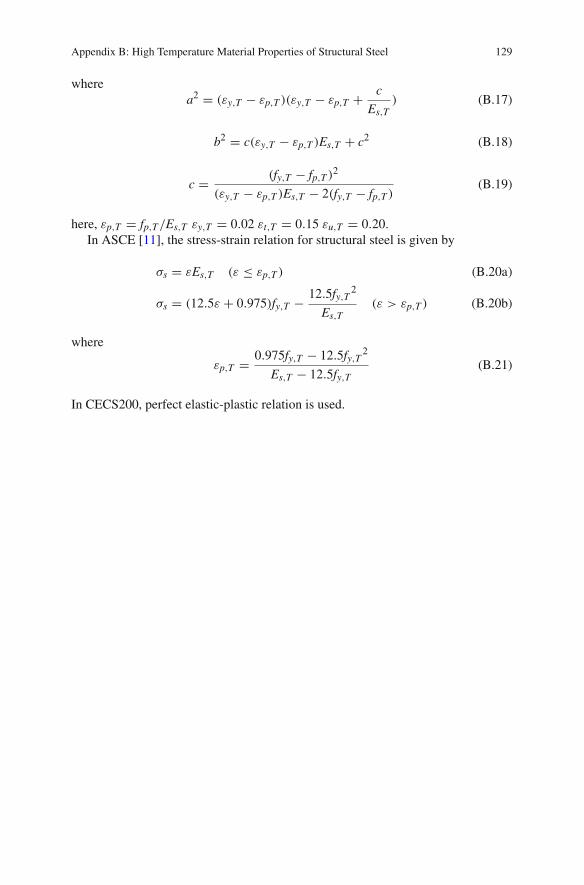
Appendix B: High Temperature Material Properties of Structural Steel 129

wherea2 = (εy,T − εp,T )(εy,T − εp,T + c

Es,T) (B.17)

b2 = c(εy,T − εp,T )Es,T + c2 (B.18)

c = (fy,T − fp,T )2

(εy,T − εp,T )Es,T − 2(fy,T − fp,T )(B.19)

here, εp,T = fp,T /Es,T εy,T = 0.02 εt,T = 0.15 εu,T = 0.20.In ASCE [11], the stress-strain relation for structural steel is given by

σs = εEs,T (ε ≤ εp,T ) (B.20a)

σs = (12.5ε + 0.975)fy,T − 12.5fy,T 2

Es,T(ε > εp,T ) (B.20b)

where

εp,T = 0.975fy,T − 12.5fy,T 2

Es,T − 12.5fy,T(B.21)

In CECS200, perfect elastic-plastic relation is used.

Appendix CCommonds for Modified One Zone Model

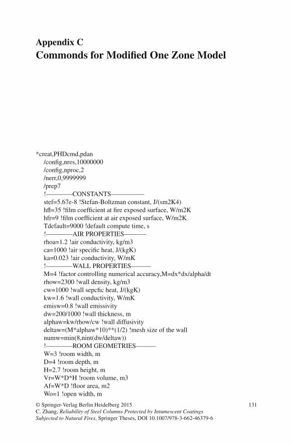
*creat,PHDcmd,pdan/config,nres,10000000/config,nproc,2/nerr,0,9999999/prep7!————CONSTANTS—————stef=5.67e-8 !Stefan-Boltzman constant, J/(sm2K4)hfl=35 !film coefficient at fire exposed surface, W/m2Khfr=9 !film coefficient at air exposed surface, W/m2KTdefault=9000 !default compute time, s!————AIR PROPERTIES———-rhoa=1.2 !air conductivity, kg/m3ca=1000 !air specific heat, J/(kgK)ka=0.023 !air conductivity, W/mK!————WALL PROPERTIES———M=4 !factor controlling numerical accuracy,M=dx*dx/alpha/dtrhow=2300 !wall density, kg/m3cw=1000 !wall sepcfic heat, J/(kgK)kw=1.6 !wall conductivity, W/mKemisw=0.8 !wall emissivitydw=200/1000 !wall thickness, malphaw=kw/rhow/cw !wall diffusivitydeltaw=(M*alphaw*10)**(1/2) !mesh size of the wallnumw=min(8,nint(dw/deltaw))!————ROOM GEOMETRIES———W=3 !room width, mD=4 !room depth, mH=2.7 !room height, mVr=W*D*H !room volume, m3Af=W*D !floor area, m2Wo=1 !open width, m


131

132 Appendix C: Commonds for Modified One Zone Model

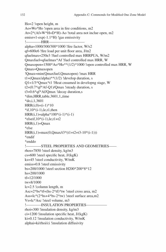
Ho=2 !open height, mAo=Wo*Ho !open area in fire conditions, m2At=2*(Af+W*H+D*H)-Ao !total area not inclue open, m2emisr=1-exp(-1.1*H) !gas emissivity!————HRR—————————–alpha=1000/300/300*1000 !fire factor, W/s2qf=600e6 !fire load per unit floor area, J/m2qfuelmax=250e3 !fuel controlled max HRRPUA, W/m2Qmaxfuel=qfuelmax*Af !fuel controlled max HRR, WQmaxopen=1500*Ao*Ho**(1/2)*1000 !open controlled max HRR, WQmax=Qmaxopen!Qmax=min(Qmaxfuel,Qmaxopen) !max HRRt1=(Qmax/alpha)**(1/2) !develop duration, sQ1=1/3*Qmax*t1 !Heat cnsumed in developng stage, Wt2=(0.7*qf*Af-Q1)/Qmax !steady duration, st3=0.6*qf*Af/Qmax !decay duration,s*dim,HRR,table,3601,1„time*do,i,1,3601HRR(i,0)=(i-1)*10*if,10*(i-1),le,t1,thenHRR(i,1)=alpha*100*(i-1)*(i-1)*elseif,10*(i-1),le,t1+t2HRR(i,1)=Qmax*elseHRR(i,1)=max(0,Qmax/t3*(t1+t2+t3-10*(i-1)))*endif*enddo!————STEEL PROPERTIES AND GEOMETRIES——rhos=7850 !steel density, kg/m3cs=600 !steel specific heat, J/(kgK)ks=45 !steel conductivity, W/mKemiss=0.8 !steel emissivitybs=200/1000 !steel section H200*200*8*12hs=200/1000tf=12/1000tw=8/1000lc=2.5 !column length, mAsc=2*bs*tf+(hs-2*tf)*tw !steel cross area, m2Ass=lc*(2*hs+4*bs-2*tw) !steel surface area,m2Vs=lc*Asc !steel volume, m3!————INSULATION PROPERTIES—————–rhoi=300 !insulation density, kg/m3ci=1200 !insulation specific heat, J/(kgK)ki=0.12 !insulation conductivity, W/mKalphai=ki/rhoi/ci !insulation diffusivity

Appendix C: Commonds for Modified One Zone Model 133

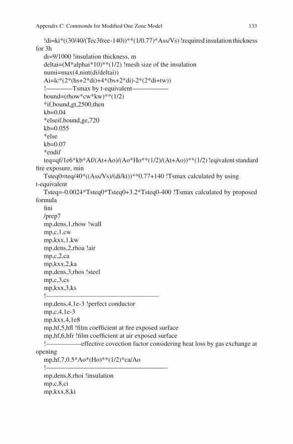
!di=ki*((30/40/(Tec3free-140))**(1/0.77)*Ass/Vs) !required insulation thicknessfor 3h

di=9/1000 !insulation thickness, mdeltai=(M*alphai*10)**(1/2) !mesh size of the insulationnumi=max(4,nint(di/deltai))Ai=lc*(2*(hs+2*di)+4*(bs+2*di)-2*(2*di+tw))!————Tsmax by t-equivalent—————–bound=(rhow*cw*kw)**(1/2)*if,bound,gt,2500,thenkb=0.04*elseif,bound,ge,720kb=0.055*elsekb=0.07*endifteq=qf/1e6*kb*Af/(At+Ao)/(Ao*Ho**(1/2)/(At+Ao))**(1/2) !eqivalent standard

fire exposure, minTsteq0=teq/40*((Ass/Vs)/(di/ki))**0.77+140 !Tsmax calculated by using

t-equivalentTsteq=-0.0024*Tsteq0*Tsteq0+3.2*Tsteq0-400 !Tsmax calculated by proposed

formulafini/prep7mp,dens,1,rhow !wallmp,c,1,cwmp,kxx,1,kwmp,dens,2,rhoa !airmp,c,2,camp,kxx,2,kamp,dens,3,rhos !steelmp,c,3,csmp,kxx,3,ks!—————————————————mp,dens,4,1e-3 !perfect conductormp,c,4,1e-3mp,kxx,4,1e8mp,hf,5,hfl !film coefficient at fire exposed surfacemp,hf,6,hfr !film coefficient at air exposed surface!—————-effective covection factor considering heat loss by gas exchange at

openingmp,hf,7,0.5*Ao*(Ho)**(1/2)*ca/Ao!——————————————————-mp,dens,8,rhoi !insulationmp,c,8,cimp,kxx,8,ki


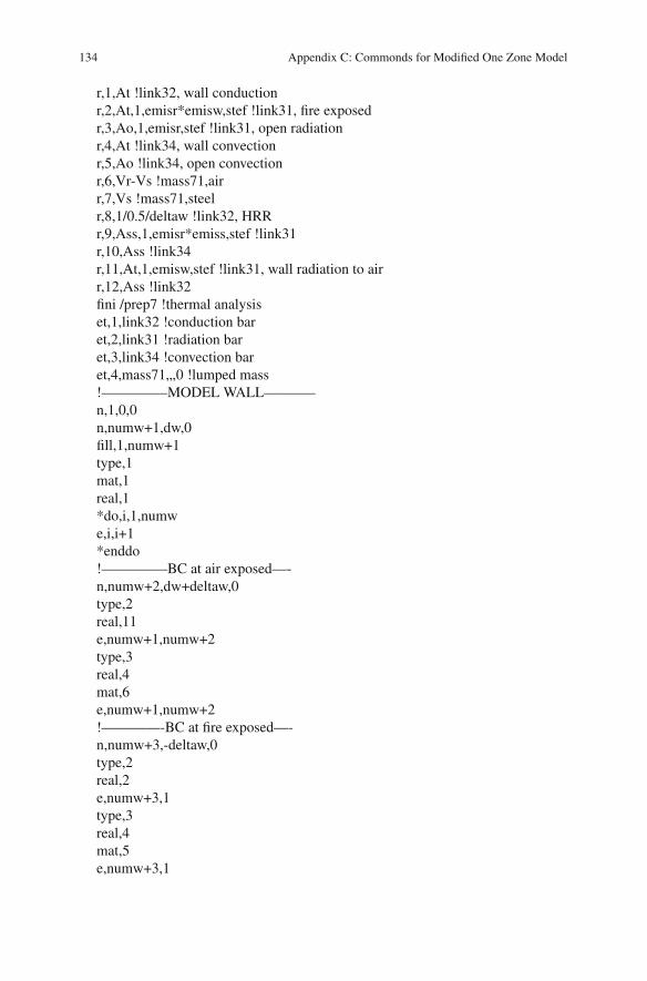
r,1,At !link32, wall conductionr,2,At,1,emisr*emisw,stef !link31, fire exposedr,3,Ao,1,emisr,stef !link31, open radiationr,4,At !link34, wall convectionr,5,Ao !link34, open convectionr,6,Vr-Vs !mass71,airr,7,Vs !mass71,steelr,8,1/0.5/deltaw !link32, HRRr,9,Ass,1,emisr*emiss,stef !link31r,10,Ass !link34r,11,At,1,emisw,stef !link31, wall radiation to airr,12,Ass !link32fini /prep7 !thermal analysiset,1,link32 !conduction baret,2,link31 !radiation baret,3,link34 !convection baret,4,mass71„,0 !lumped mass!————–MODEL WALL———–n,1,0,0n,numw+1,dw,0fill,1,numw+1type,1mat,1real,1*do,i,1,numwe,i,i+1*enddo!————–BC at air exposed—-n,numw+2,dw+deltaw,0type,2real,11e,numw+1,numw+2type,3real,4mat,6e,numw+1,numw+2!————-BC at fire exposed—-n,numw+3,-deltaw,0type,2real,2e,numw+3,1type,3real,4mat,5e,numw+3,1

Appendix C: Commonds for Modified One Zone Model 135

!————-BC at opening———-type,2real,3n,numw+4,-deltaw,-deltawe,numw+3,numw+4type,3mat,7real,5e,numw+3,numw+4!————-HEAT FLUX TO STEEL—–n,numw+5,-deltaw,deltawn,numw+5+numi,-deltaw,deltaw+difill,numw+5,numw+5+numitype,1real,12mat,8*do,i,1,numie,numw+5+i-1,numw+5+i*enddotype,2real,9e,numw+3,numw+5type,3real,10mat,5e,numw+3,numw+5!————–LUMPED MASS————-type,4mat,2real,6e,numw+3mat,3real,7e,numw+5+numi!————–MODEL HRR—————n,numw+6+numi,-1.5*deltaw,0type,1mat,4real,8e,numw+6+numi,numw+3!————–HEAT LOADING————toffset,273tunif,20esel,s,mat„4bfe,all,hgen„


d,numw+2,temp,20d,numw+4,temp,20fini/soluantype,4autots,ondeltim,10,1,100time,Tdefaultoutres,nsol,allallselsolvefini/post26nsol,2,numw+5+numi,tempstore,merge*GET,size,VARI„NSETS*dim,TsFEM,array,size,1vget,TsFEM(1),2*vscfun,TsmaxFEM,max,TsFEMbeta1=Tsteq0-TsmaxFEMbeta2=Tsteq-TsmaxFEMfini*end/inp,PHDcmd,pdan/pdspdanl,PHDcmd,pdanPDVAR,qf,LOG1,600e6,240e6 !PDF of fire load, GaussianPDVAR,alpha,GAUS,0.012*1000,0.003*1000 !PDF of growth fire coefficient,

GaussianPDVAR,Ao,GAUS,2,2*0.2 !PDF of coefficient considering the opening of win-

dows in fire, TGAUPDVAR,kw,GAUS,1.6,0.16PDVAR,dw,GAUS,200/1000,200/1000*0.1PDVAR,ki,GAUS,0.12,0.12*0.3PDVAR,di,LOG1,9/1000,9/1000*0.2PDVAR,Tsteq0,respPDVAR,Tsteq,respPDVAR,TsmaxFEM,respPDVAR,beta1,respPDVAR,beta2,respPDMETH,MCS,LHSPDLHS,200,1„„„,INITPDEXE,MCStri„1e7

Appendix DCommonds for Monte Carlo Simulations

function y=NbT(fy20,e20,T,bs,hs,tw,tf,lc)Asc=2*bs*tf+(hs-2*tf)*tw;Ixx=(bs*hs∧3-(bs-tw)*(hs-2*tf)∧3)/12;Iyy=(2*tf*bs∧3+(hs-2*tf)*tw∧3)/12;ix=sqrt(Ixx/Asc);iy=sqrt(Iyy/Asc);lambdax=lc/ix;lambday=lc/iy;lambda20=lambday;lambdaE20=lambda20/3.14*sqrt(fy20/e20);if T<100ered=1;elseif T<500ered=-0.001*T+1.1;elseif T<600ered=-0.0029*T+2.05;elseif T<700ered=-0.0018*T+1.39;elseif T<800ered=-0.0004*T+0.41;elseif T<1200ered=-0.000225*T+0.27;elseered=0;endeT=e20*ered;if T<=400fyred=1;elseif T<500


137

138 Appendix D: Commonds for Monte Carlo Simulations

fyred=-0.0022*T+1.88;elseif T<600fyred=-0.0031*T+2.33;elseif T<700fyred=-0.0024*T+1.91;elseif T<800fyred=-0.0012*T+1.07;elseif T<900fyred=-0.0005*T+0.51;elseif T<1200fyred=-0.0002*T+0.24;elsefyred=0;endfyT=fy20*fyred;lambdaET=lambdaE20*sqrt(fyred/ered);betaT=0.65;alphaT=betaT*sqrt(235/fy20);phiT=0.5*(1+alphaT*lambdaET+lambdaET∧2);chiT=min(1,1/(phiT+sqrt(phiT∧2-lambdaET∧2)));NbT=chiT*Asc*fyT;y=NbT;function [AB]=MCS(Wi,Di,Hi,Woi,Hoi,qf0,Ri0,fy20,e20,mu0,Nb0,bs0,hs0,tw0,tf0,lc0)N=1000000;qf=lognrnd(log(qf0∧2/((qf0*0.3)∧2+qf0∧2)∧0.5),(log((0.3*qf0)∧2/qf0∧2+1))∧0.5,N,1);Ri=lognrnd(log(Ri0∧2/((Ri0*0.3)∧2+Ri0∧2)∧0.5),(log((0.3*Ri0)∧2/Ri0∧2+1))∧0.5,N,1);zeta=lognrnd(log(0.2∧2/((0.2*1)∧2+0.2∧2)∧0.5),(log((1*0.2)∧2/0.2∧2+1))∧0.5,N,1);b=normrnd(2014,2014*0.09,N,1);kb=ones(N,1);for i=1:Nif b(i)>2500kb(i)=0.04;elseif b(i)<=2500kb(i)=0.055;elsekb(i)=0.07;endendW=Wi.*ones(N,1);D=Di.*ones(N,1);H=Hi.*ones(N,1);Wo=Woi.*ones(N,1);Ho=Hoi.*ones(N,1);Af=W.*D;At=2.*(W.*D+W.*H+D.*H);Ao=Wo.*Ho;OF=Ao.*Ho.∧0.5./At;

Appendix D: Commonds for Monte Carlo Simulations 139

wf=(OF.*(1-zeta)).∧(-0.5).*Af./At;teq=qf.*kb.*wf;lc=normrnd(lc0,lc0*0.05,N,1);fy20=normrnd(fy20,fy20*0.063,N,1);e20=normrnd(e20,e20*0.045,N,1);bs=normrnd(bs0,bs0*0.05,N,1);hs=normrnd(hs0,hs0*0.05,N,1);tw=normrnd(tw0,tw0*0.05,N,1);tf=normrnd(tf0,tf0*0.05,N,1);C=4.*bs-2.*tw+2.*hs;As=2.*bs.*tw+tw.*(hs-2.*tf);AiV=C./As.*1000;Iyy=(2.*tf.*bs.∧3+(hs-2.*tf).*tw.∧3)./12;iyy=(Iyy./As).∧0.5;lambday=lc./iyy;lambdaE=lambday./3.14.*(fy20./e20).∧0.5;alpha=0.65.*(235./fy20).∧0.5;phi=(1+alpha.*lambdaE+lambdaE.∧2)./2;chi=1./(phi+(phi.∧2-lambdaE.∧2).∧0.5);Nb=chi.*As.*fy20;PT=normrnd(mu0*Nb0,mu0*Nb0*0.3,N,1);mu=PT./Nb;PF1=lognrnd(-0.053455,0.121189,N,1);PF2=evrnd(1.00378,0.0954518,N,1);Tb=PF2.*(39.19.*log(1/0.9674./mu.∧3.833-1)+482);Delta=teq./40.*(AiV./Ri).∧0.77;Tsmax=PF1.*(-0.0024.*Delta.∧2+2.528.*Delta+0.96);n=0;m=0;for i=1:Nif Tsmax(i)>=300&&Tsmax(i)<=600if Tb(i)<=Tsmax(i)n=n+1;elsen=n;endm=m;elsem=m+1;endendPfail=n/(N-m);Beta=norminv(1-Pfail,0,1);A=Pfail;B=Beta;

140 Appendix D: Commonds for Monte Carlo Simulations

References

1. J. Holman, Heat Tranfer, 6th edn. (McGraw-Hill, New York, 1986)2. D. Drysdale, An Introduction to Fire Dynamics, 2nd edn. (Wiley, New York, 1999)3. J. Rockett, J. Mike, SFPE Handbbok of Fire Protection Engineering Society of Fire Protection

Engineers, 2002), 3rd edn., chap. Section 1–2: Condction of Heat in Solids4. A. Jowsey, Fire Imposed Heat Fluxes For Structural Analysis. Ph.D. thesis (The University of

Edinburgh, 2006)5. B. McCaffrey, J. Quintiere, M. Harkleroad, Fire Technology 17(2), 98 (1981)6. J.H. Lienhard IV, J.H. Lienhard V, A Heat Transfer Textbook, 3rd edn. (Phlogiston Press,

Cambridge, Massachusetts, 2003)7. R. Siegel, J. Howell, Thermal Radiation Heat Transfer, 3rd edn. (Hemisphere Publishing Cor-

poration, Washington DC, 1992)8. BSI, Eurocode 4: Design of Composite Steel and Concrete Structures—Part 1–2: General

Rules—Structural Fire Design (British Standard, 2005)9. M.F. Modest, Heat Transfer Handbook (Wiley, New York, 2003), (chap. Section 8: Thermal

radiation)10. BSI,Eurocode 3: Design of Steel Structures—Part 1–2: General Rules—StrUctural Fire Design

(British Standard, 2005)11. ASCE, Structural Fire Protection (ASCECommittee on fire protection,Manual No.78, Reston,

VA, 1992)12. China Association for Engineering Construction Standardization (CECS200), Technical Code

for Fire Safety of Steel Structure in Buildings (Beijing, China Planning Press, 2006)

Appendix A Fundamentals of Heat Transfer - Springer978-3-662-46379-6/1.pdfAppendix A Fundamentals of...

Documents

Transcript of Appendix A Fundamentals of Heat Transfer - Springer978-3-662-46379-6/1.pdfAppendix A Fundamentals of...