λ,µ,ρ,An,Wn,L t ,L,L ,w,w - School of Computer Sciencedobo/2460/queuing.pdfA tool crib has...
21
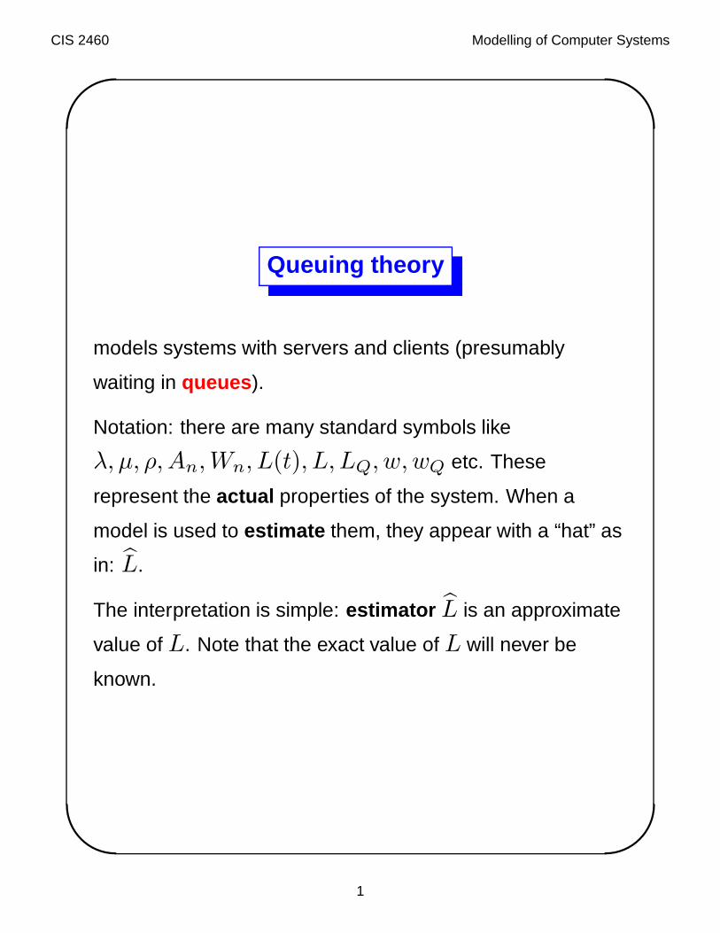
CIS 2460 Modelling of Computer Systems ✬ ✫ ✩ ✪ Queuing theory models systems with servers and clients (presumably waiting in queues). Notation: there are many standard symbols like λ, μ, ρ, A n ,W n ,L(t), L, L Q ,w,w Q etc. These represent the actual properties of the system. When a model is used to estimate them, they appear with a “hat” as in: L. The interpretation is simple: estimator L is an approximate value of L. Note that the exact value of L will never be known. 1
Transcript of λ,µ,ρ,An,Wn,L t ,L,L ,w,w - School of Computer Sciencedobo/2460/queuing.pdfA tool crib has...
CIS 2460 Modelling of Computer Systems'
&
$
%
Queuing theory
models systems with servers and clients (presumably
waiting in queues).
Notation: there are many standard symbols like
λ, µ, ρ, An, Wn, L(t), L, LQ, w, wQ etc. These
represent the actual properties of the system. When a
model is used to estimate them, they appear with a “hat” as
in: L.
The interpretation is simple: estimator L is an approximate
value of L. Note that the exact value of L will never be
known.
1
CIS 2460 Modelling of Computer Systems'
&
$
%
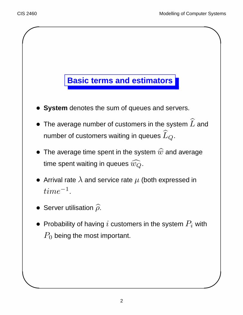
Basic terms and estimators
• System denotes the sum of queues and servers.
• The average number of customers in the system L and
number of customers waiting in queues LQ.
• The average time spent in the system w and average
time spent waiting in queues wQ.
• Arrival rate λ and service rate µ (both expressed in
time−1.
• Server utilisation ρ.
• Probability of having i customers in the system Pi with
P0 being the most important.
2
CIS 2460 Modelling of Computer Systems'
&
$
%
The system and its model
The standard assumption is that the “system” starts its
operation at time 0 and works forever. Thus we will not know
the true properties of the system until the end of time
(whatever that means).
In a model, we use the information gathered so far, i.e. from
time 0 to time T (T is just a symbolic notation). The model
yields some statistics; the larger T is, the closer these
statistics are to the real ones.
Mathematically speaking: if L is the average number of
customers in the system and L is the number that came out
of the model, then:
limT→∞
L = L
The same applies to all estimators.
3
CIS 2460 Modelling of Computer Systems'
&
$
%
Average number of customers
In the actual system the number of customers in the system
is given by the function L(t). Obviously we do not know this
function in its analytical form. The average number of
customers in the real system is:
L = limt→∞
∫ t
0
L(x)dx
4
CIS 2460 Modelling of Computer Systems'
&
$
%
In the model, we know what happened in the period [0, T ].
The number of customers varied in time, but their number at
any moment can be recorded and then tallied up. For each
number of customers i (where 0 ≤ i < ∞) the lengths of
the time intervals when there were precisely i customers in
the system are added together giving a total time Ti Clearly:
∞∑
i=0
Ti = T
The estimator L for the average number of customers is a
weighted average (weights are time durations):
L =1
T
∞∑
i=0
iTi =∞∑
i=0
iTi
T
Note that the right formula looks like the mean of a pdf.
5
CIS 2460 Modelling of Computer Systems'
&
$
%
What we are interested in is L. What we have is L.
It is easy to see that
L =1
T
∫ T
0
L(t)dt
(even though we do not know how L(t) looks like).
Since
L = limt→∞
∫ t
0
L(x)dx
it is obvious that:
limT→∞
L = L
6
CIS 2460 Modelling of Computer Systems'
&
$
%
Average time spent in the system
The average time spent in the system is denoted by w and
is impossible to determine in finite time.
In the model, we can record the times spent in the system of
all the customers that left before time T . Let these times be
W1, W2, · · · , Wn where n is the number of arrivals (or
departures) in the period [0, T ].
An estimator for w is:
w =1
n
n∑
i=1
Wi
As in the case of the number of customers,
limn→∞
w = w
This is true for all “real” cases, but not “mathematically” as
there are some weird (and unrealistic) counterexamples.
7
CIS 2460 Modelling of Computer Systems'
&
$
%
Little’s law
In the model, the arrival rate is nT . We denote this rate by λ
because it is an estimator of the true arrival rate λ.
The conservation law (Little’s) gives the following
relationship:
L = λw
Not surprisingly, Little’s law holds for the real system:
L = λw
but this is purely for the record, because we have no means
to compute L or w.
8
CIS 2460 Modelling of Computer Systems'
&
$
%
Server utilisation
Let µ be the service rate (as in “can handle µ customers per
minute”). Note that 1µ is the average service time.
If µ < λ the system eventually explodes, because the
waiting queue grows to infinity.
A system can be stable only if λ < µ. In that case, the
server rate should be split into two parts: the part when the
server is “busy” and the remainder, when the server is “idle.”
The busy part obviously is equal to the arrival rate λ
because th e server is busy if and only if there is a customer
around.
Hence the server utilisation ρ (“the busy part”) equals:
ρ =λ
µ
If the system has c identical servers, the same rule holds:
ρ =λ
cµλ < cµ
9
CIS 2460 Modelling of Computer Systems'
&
$
%
Types of queuing systems
Kendall proposed a unified notation describing the
properties of a given queuing system: A/B/c/N/K,
where the letters represent:
A interarrival–time distribution
B service–time distribution
c the number of parallel servers
N the system capacity
K the size of the customer population.
10
CIS 2460 Modelling of Computer Systems'
&
$
%
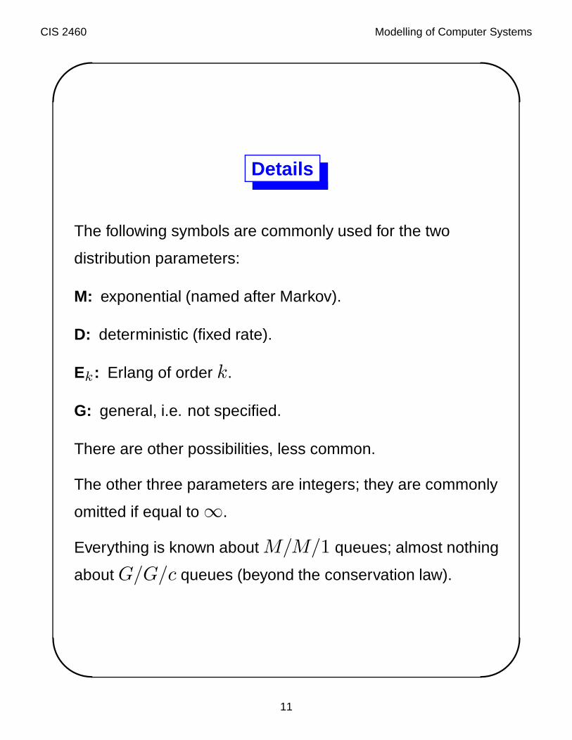
Details
The following symbols are commonly used for the two
distribution parameters:
M: exponential (named after Markov).
D: deterministic (fixed rate).
Ek: Erlang of order k.
G: general, i.e. not specified.
There are other possibilities, less common.
The other three parameters are integers; they are commonly
omitted if equal to ∞.
Everything is known about M/M/1 queues; almost nothing
about G/G/c queues (beyond the conservation law).
11
CIS 2460 Modelling of Computer Systems'
&
$
%
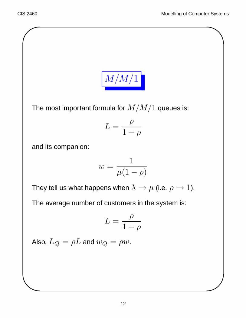
M/M/1
The most important formula for M/M/1 queues is:
L =ρ
1 − ρ
and its companion:
w =1
µ(1 − ρ)
They tell us what happens when λ → µ (i.e. ρ → 1).
The average number of customers in the system is:
L =ρ
1 − ρ
Also, LQ = ρL and wQ = ρw.
12
CIS 2460 Modelling of Computer Systems'
&
$
%
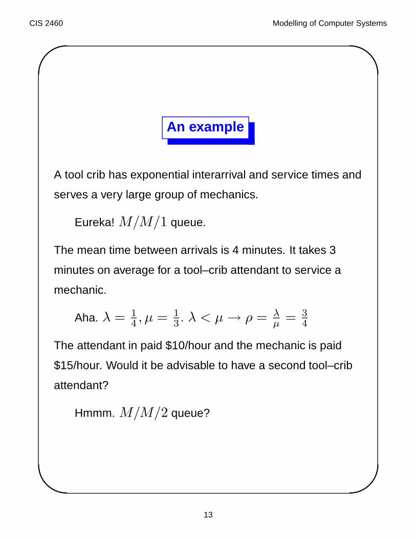
An example
A tool crib has exponential interarrival and service times and
serves a very large group of mechanics.
Eureka! M/M/1 queue.
The mean time between arrivals is 4 minutes. It takes 3
minutes on average for a tool–crib attendant to service a
mechanic.
Aha. λ = 14 , µ = 1
3 . λ < µ → ρ = λµ = 3
4
The attendant in paid $10/hour and the mechanic is paid
$15/hour. Would it be advisable to have a second tool–crib
attendant?
Hmmm. M/M/2 queue?
13
CIS 2460 Modelling of Computer Systems'
&
$
%
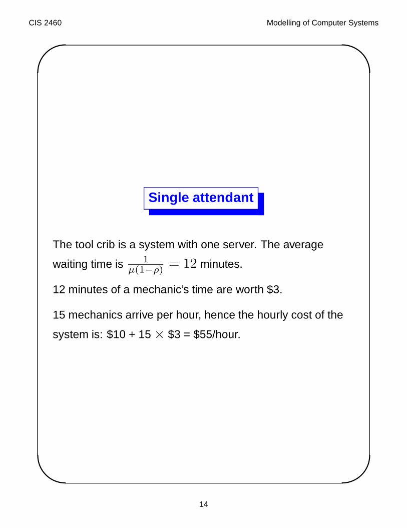
Single attendant
The tool crib is a system with one server. The average
waiting time is 1µ(1−ρ) = 12 minutes.
12 minutes of a mechanic’s time are worth $3.
15 mechanics arrive per hour, hence the hourly cost of the
system is: $10 + 15 × $3 = $55/hour.
14
CIS 2460 Modelling of Computer Systems'
&
$
%
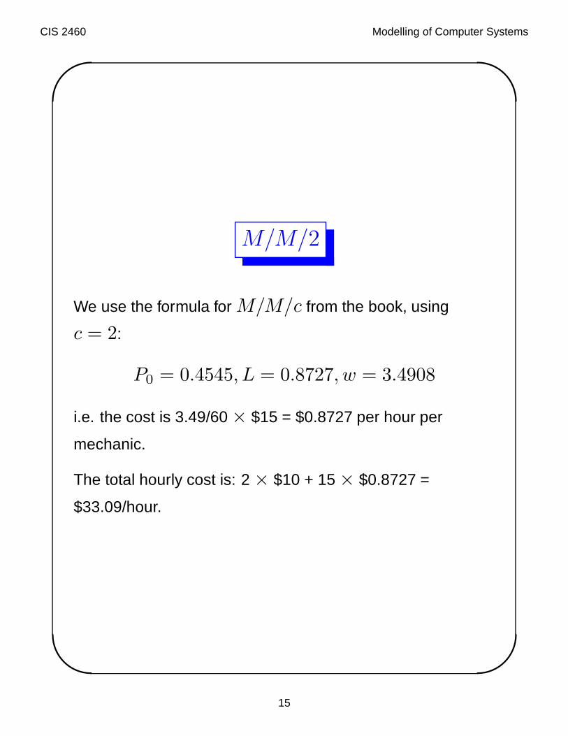
M/M/2
We use the formula for M/M/c from the book, using
c = 2:
P0 = 0.4545, L = 0.8727, w = 3.4908
i.e. the cost is 3.49/60 × $15 = $0.8727 per hour per
mechanic.
The total hourly cost is: 2 × $10 + 15 × $0.8727 =
$33.09/hour.
15
CIS 2460 Modelling of Computer Systems'
&
$
%
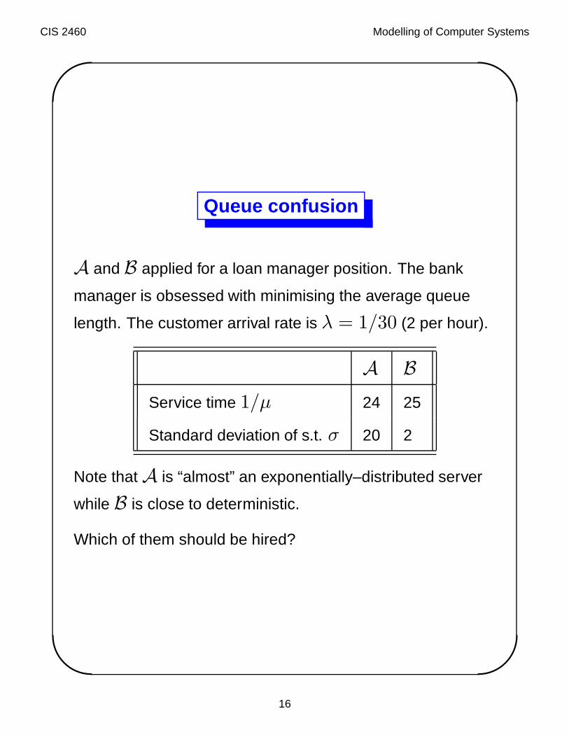
Queue confusion
A and B applied for a loan manager position. The bank
manager is obsessed with minimising the average queue
length. The customer arrival rate is λ = 1/30 (2 per hour).
A B
Service time 1/µ 24 25
Standard deviation of s.t. σ 20 2
Note that A is “almost” an exponentially–distributed server
while B is close to deterministic.
Which of them should be hired?
16
CIS 2460 Modelling of Computer Systems'
&
$
%
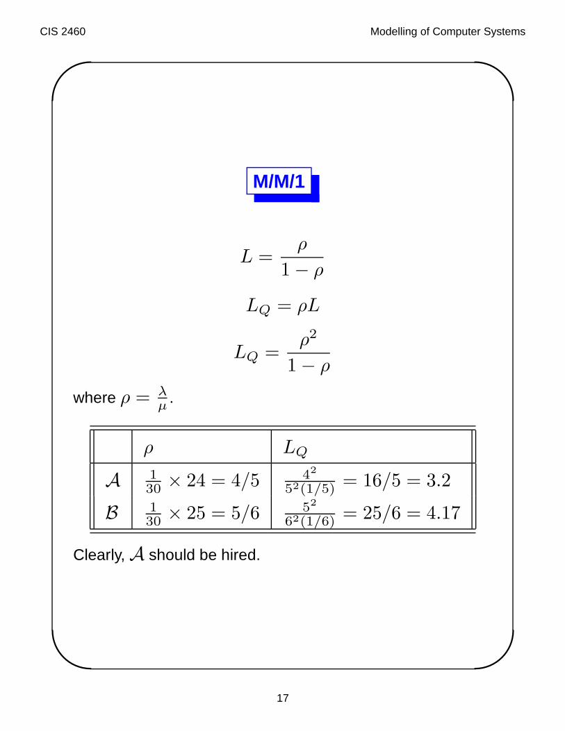
M/M/1
L =ρ
1 − ρ
LQ = ρL
LQ =ρ2
1 − ρ
where ρ = λµ .
ρ LQ
A 130 × 24 = 4/5 42
52(1/5) = 16/5 = 3.2
B 130 × 25 = 5/6 52
62(1/6) = 25/6 = 4.17
Clearly, A should be hired.
17
CIS 2460 Modelling of Computer Systems'
&
$
%
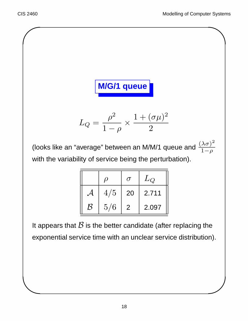
M/G/1 queue
LQ =ρ2
1 − ρ×
1 + (σµ)2
2
(looks like an “average” between an M/M/1 queue and(λσ)2
1−ρ
with the variability of service being the perturbation).
ρ σ LQ
A 4/5 20 2.711
B 5/6 2 2.097
It appears that B is the better candidate (after replacing the
exponential service time with an unclear service distribution).
18
CIS 2460 Modelling of Computer Systems'
&
$
%
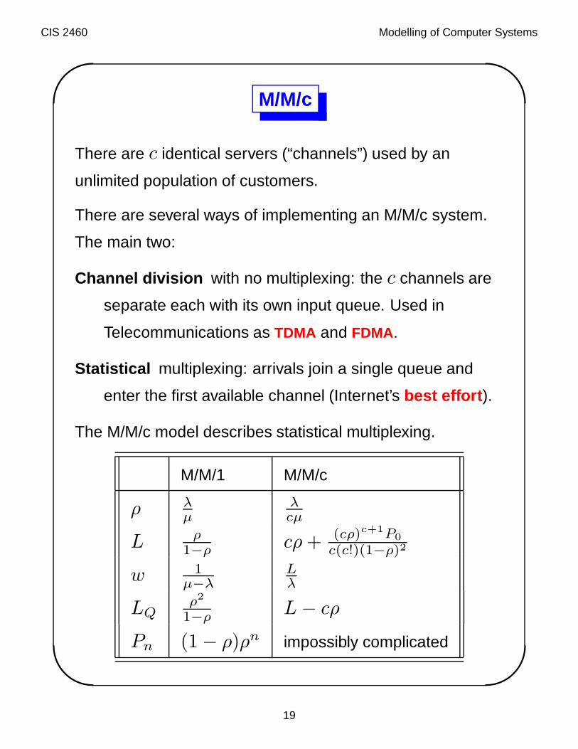
M/M/c
There are c identical servers (“channels”) used by an
unlimited population of customers.
There are several ways of implementing an M/M/c system.
The main two:
Channel division with no multiplexing: the c channels are
separate each with its own input queue. Used in
Telecommunications as TDMA and FDMA.
Statistical multiplexing: arrivals join a single queue and
enter the first available channel (Internet’s best effort).
The M/M/c model describes statistical multiplexing.
M/M/1 M/M/c
ρ λµ
λcµ
L ρ1−ρ cρ + (cρ)c+1P0
c(c!)(1−ρ)2
w 1µ−λ
Lλ
LQρ2
1−ρ L − cρ
Pn (1 − ρ)ρn impossibly complicated
19
CIS 2460 Modelling of Computer Systems'
&
$
%
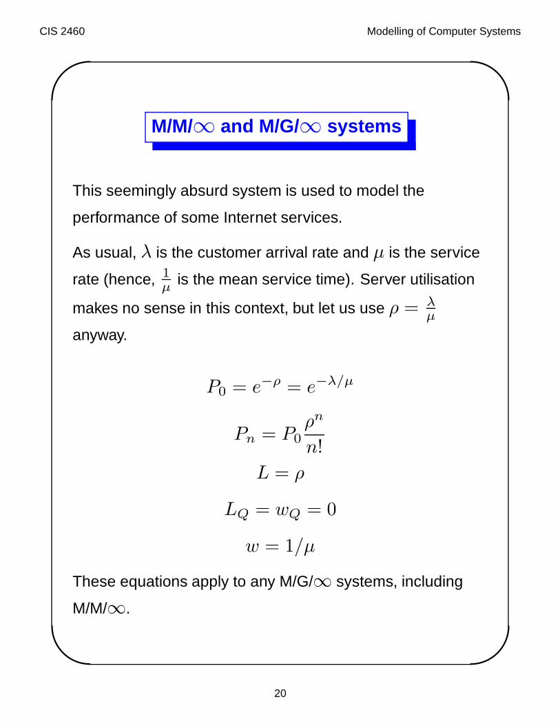
M/M/∞ and M/G/∞ systems
This seemingly absurd system is used to model the
performance of some Internet services.
As usual, λ is the customer arrival rate and µ is the service
rate (hence, 1µ is the mean service time). Server utilisation
makes no sense in this context, but let us use ρ = λµ
anyway.
P0 = e−ρ = e−λ/µ
Pn = P0ρn
n!
L = ρ
LQ = wQ = 0
w = 1/µ
These equations apply to any M/G/∞ systems, including
M/M/∞.
20
CIS 2460 Modelling of Computer Systems'
&
$
%
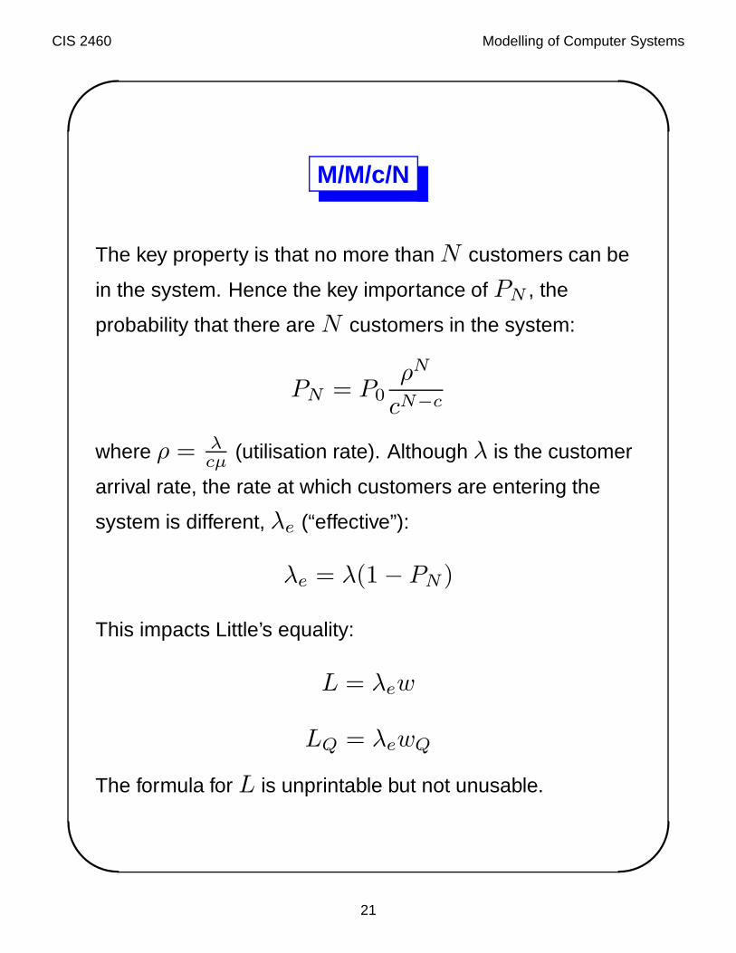
M/M/c/N
The key property is that no more than N customers can be
in the system. Hence the key importance of PN , the
probability that there are N customers in the system:
PN = P0ρN
cN−c
where ρ = λcµ (utilisation rate). Although λ is the customer
arrival rate, the rate at which customers are entering the
system is different, λe (“effective”):
λe = λ(1 − PN )
This impacts Little’s equality:
L = λew
LQ = λewQ
The formula for L is unprintable but not unusable.
21