Anastasia Fialkov - Max Planck Society · Anastasia Fialkov Tel Aviv University MPIK 29.10.2012...
64
Anastasia Fialkov Tel Aviv University MPIK 29.10.2012 Credit: WMAP team Based on: AF, Itzhaki, Kovetz (JCAP 2010) Rathaus, AF, Itzhaki (JCAP 2011)
Transcript of Anastasia Fialkov - Max Planck Society · Anastasia Fialkov Tel Aviv University MPIK 29.10.2012...
Anastasia FialkovTel Aviv University
MPIK 29.10.2012
Credit: WMAP team
Based on:
AF, Itzhaki, Kovetz (JCAP 2010)
Rathaus, AF, Itzhaki (JCAP 2011)
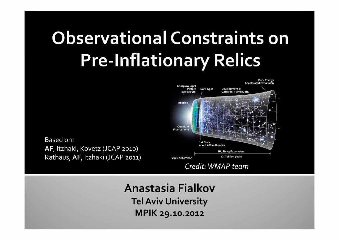
• Inflation is a period of ~ exponential expansion.
• Simplest model:
scalar field (inflaton, φ) slowly rolls down a ~ flat potential
Initial Conditionsfor structure formation:
Quantum fluctuations → classical Comoving
scale
Comoving
Hubble
Horizon
Inflation
Time
Observable
Window
Credit: WMAP team
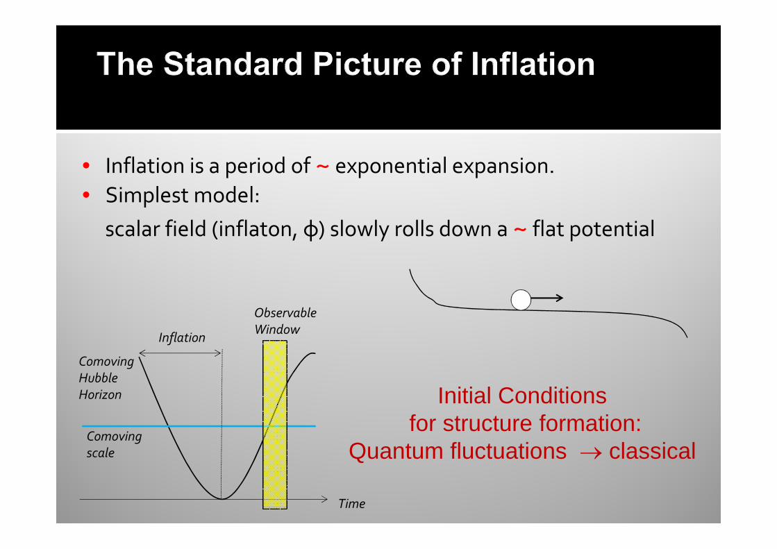
Image: Loeb, Scientific American 2006
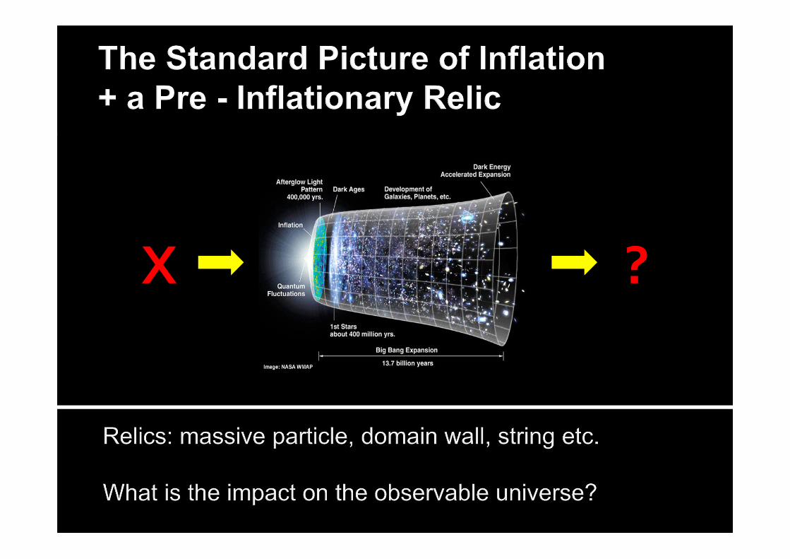
X ?
Credit: WMAP team
X ?
Credit: WMAP team
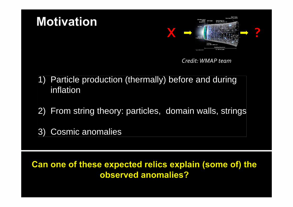
1) Particle production (thermally) before and during inflation
2) From string theory: particles, domain walls, strings
3) Cosmic anomalies
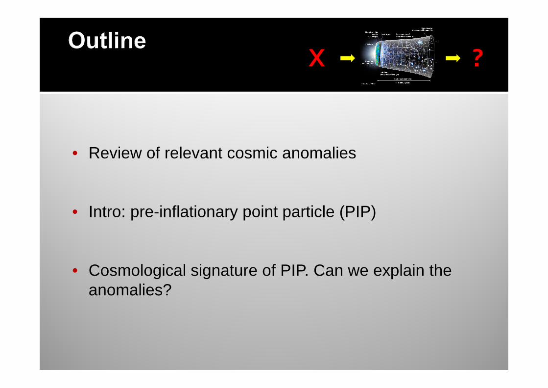
• Review of relevant cosmic anomalies
• Intro: pre-inflationary point particle (PIP)
• Cosmological signature of PIP. Can we explain the anomalies?
X ?
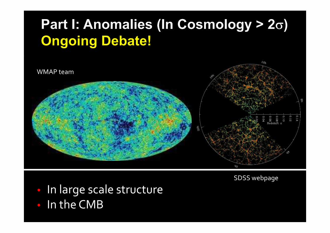
• In large scale structure
• In the CMB
WMAP team
SDSS webpage
WMAP team
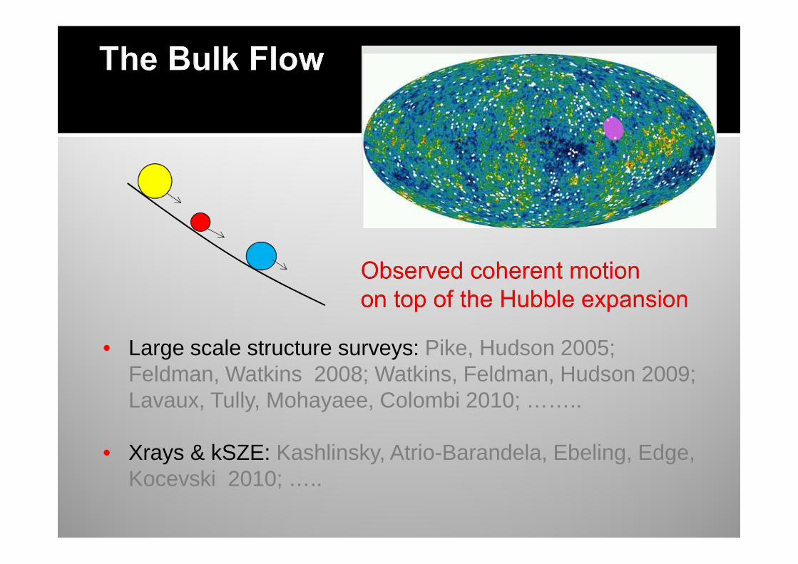
• Large scale structure surveys: Pike, Hudson 2005; Feldman, Watkins 2008; Watkins, Feldman, Hudson 2009; Lavaux, Tully, Mohayaee, Colombi 2010; ……..
• Xrays & kSZE: Kashlinsky, Atrio-Barandela, Ebeling, Edge, Kocevski 2010; …..
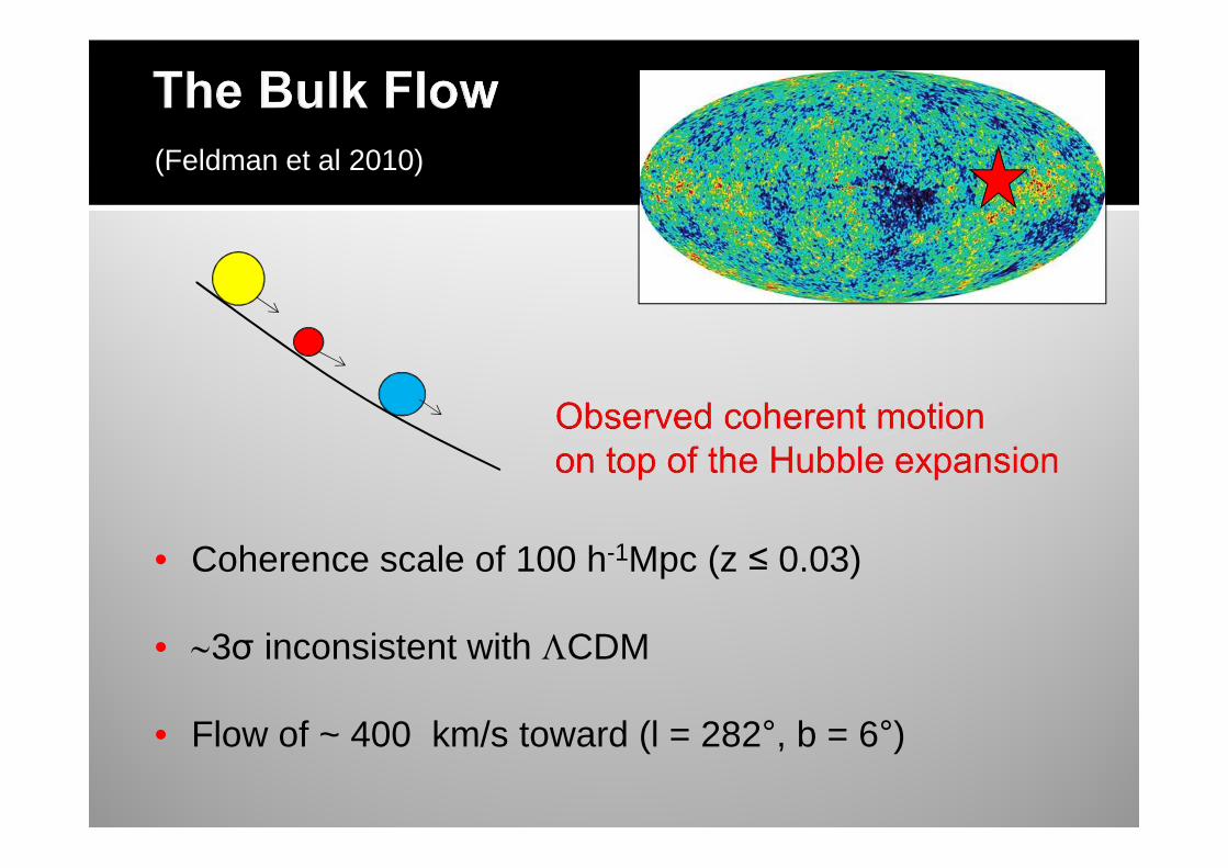
• Coherence scale of 100 h-1Mpc (z ≤ 0.03)
• ∼3σ inconsistent with ΛCDM
• Flow of ~ 400 km/s toward (l = 282°, b = 6°)
(Feldman et al 2010)
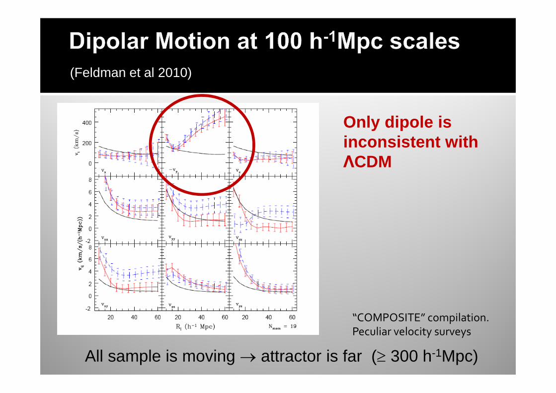
“COMPOSITE” compilation. Peculiar velocity surveys
All sample is moving → attractor is far (≥ 300 h-1Mpc)
Only dipole is inconsistent with ΛCDM
(Feldman et al 2010)
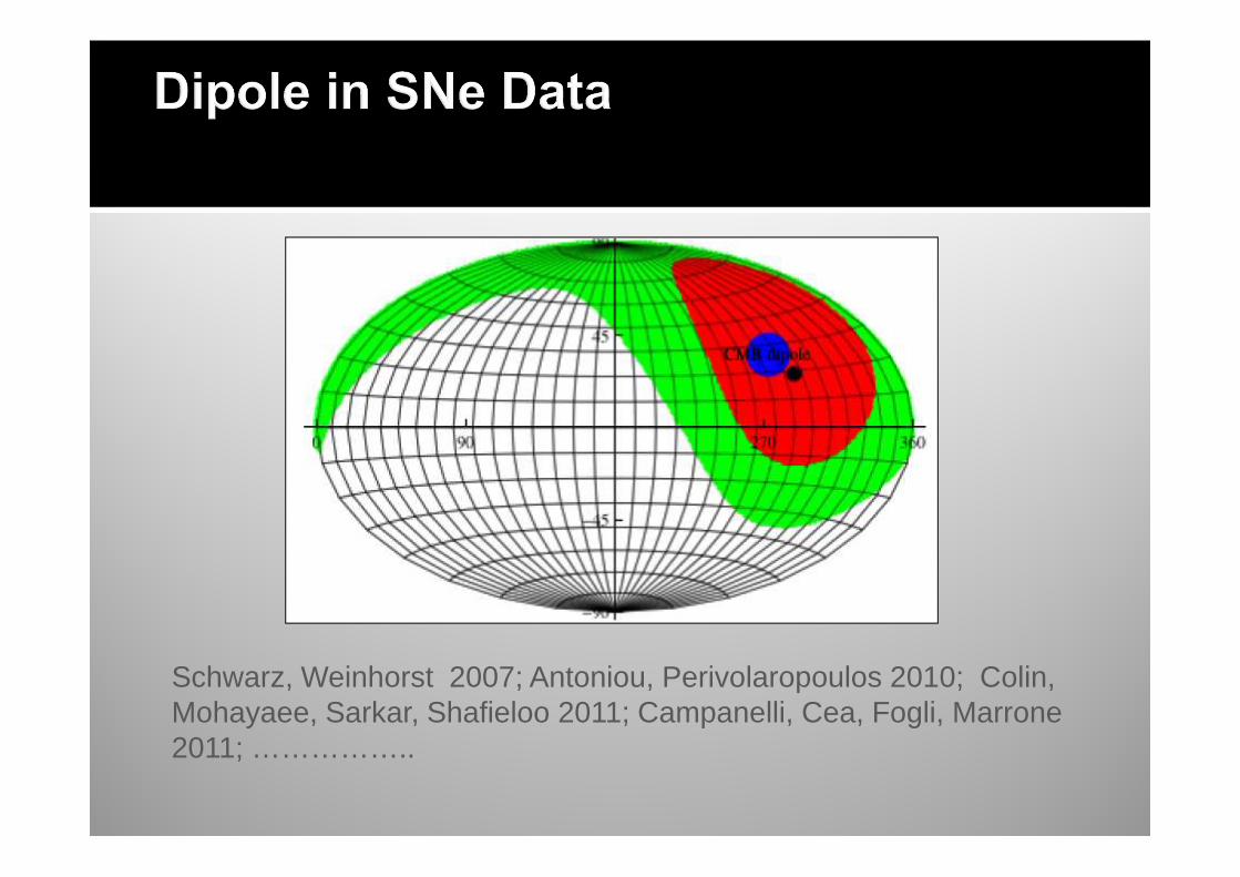
Schwarz, Weinhorst 2007; Antoniou, Perivolaropoulos 2010; Colin, Mohayaee, Sarkar, Shafieloo 2011; Campanelli, Cea, Fogli, Marrone2011; ……………..
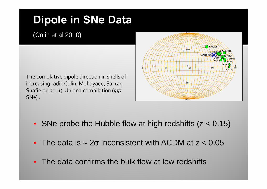
• SNe probe the Hubble flow at high redshifts (z < 0.15)
• The data is ∼ 2σ inconsistent with ΛCDM at z < 0.05
• The data confirms the bulk flow at low redshifts
The cumulative dipole direction in shells of
increasing radii. Colin, Mohayaee, Sarkar,
Shafieloo 2011) Union2 compilation (557
SNe) .
(Colin et al 2010)
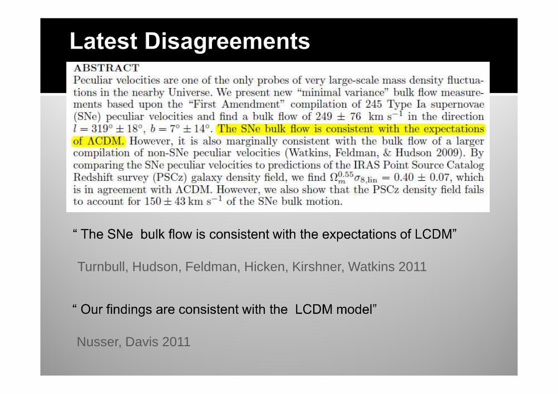
Nusser, Davis 2011
Turnbull, Hudson, Feldman, Hicken, Kirshner, Watkins 2011
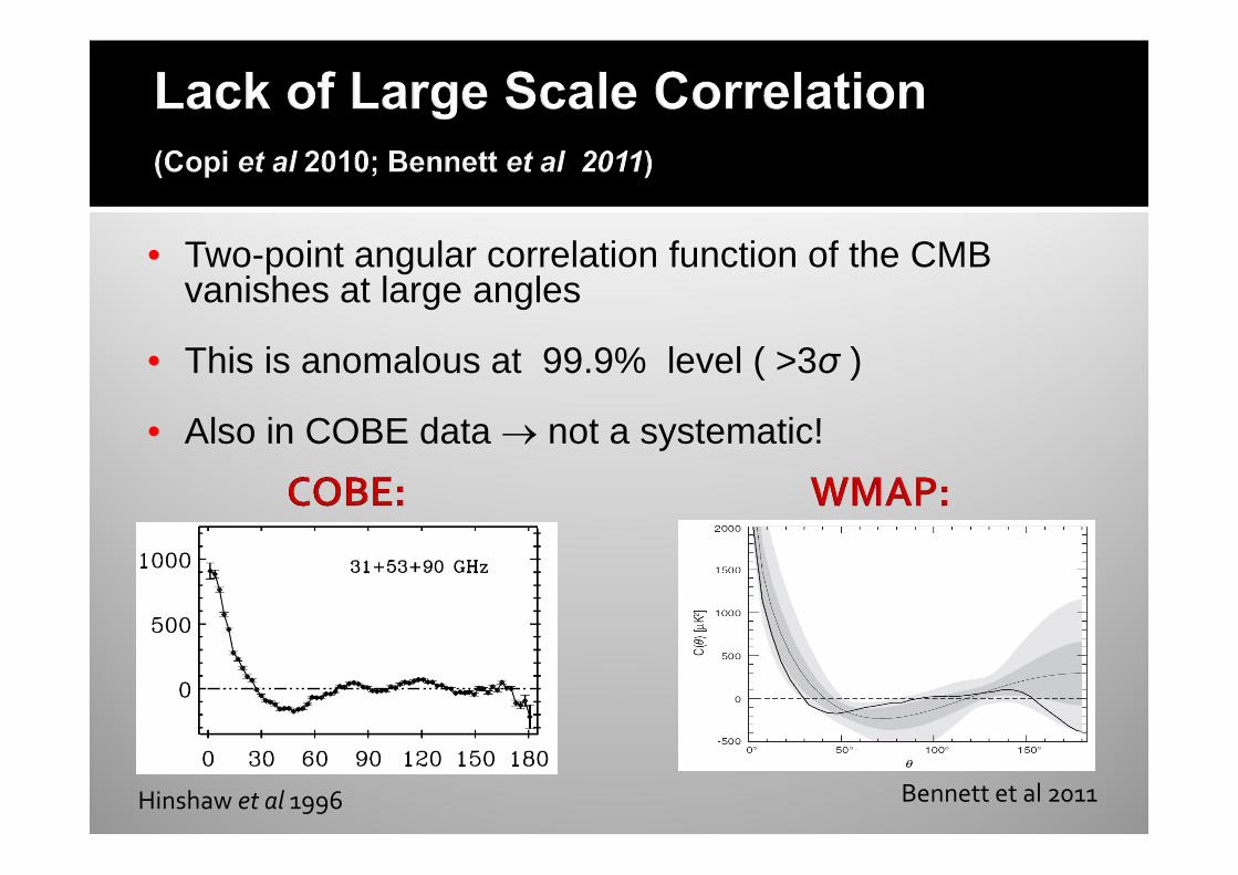
• Two-point angular correlation function of the CMB vanishes at large angles
• This is anomalous at 99.9% level ( >3σ )
• Also in COBE data → not a systematic!
Bennett et al 2011Hinshaw et al 1996
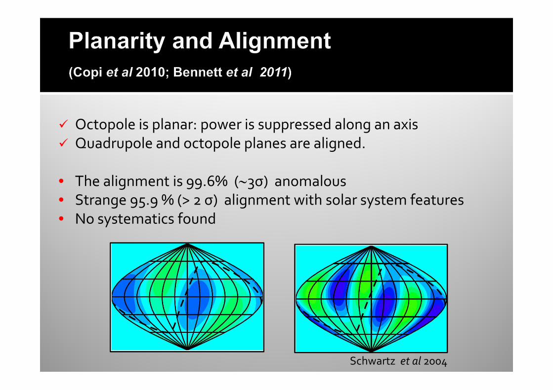
� Octopole is planar: power is suppressed along an axis
� Quadrupole and octopole planes are aligned.
• The alignment is 99.6% (∼3σ) anomalous• Strange 95.9 % (> 2 σ) alignment with solar system features
• No systematics found
Schwartz et al 2004
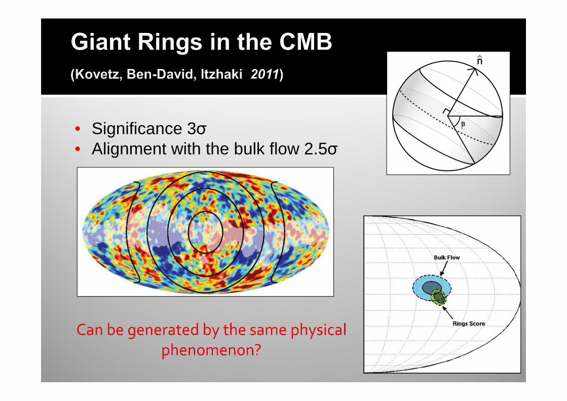
• Significance 3σ• Alignment with the bulk flow 2.5σ
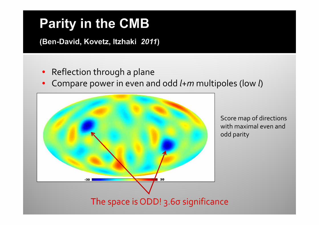
• Reflection through a plane
• Compare power in even and odd l+m multipoles (low l)
Score map of directions
with maximal even and odd parity
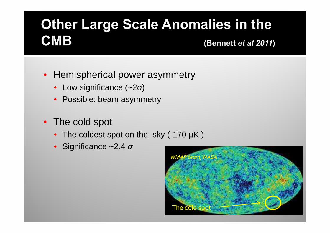
• Hemispherical power asymmetry• Low significance (~2σ)• Possible: beam asymmetry
• The cold spot• The coldest spot on the sky (-170 µK )• Significance ~2.4 σ
The cold spot
WMAP team, NASA
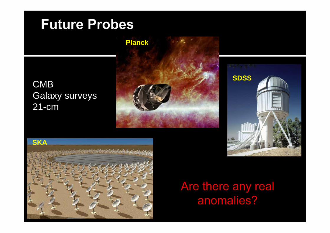
CMB Galaxy surveys21-cm
SDSS
SKA
Planck
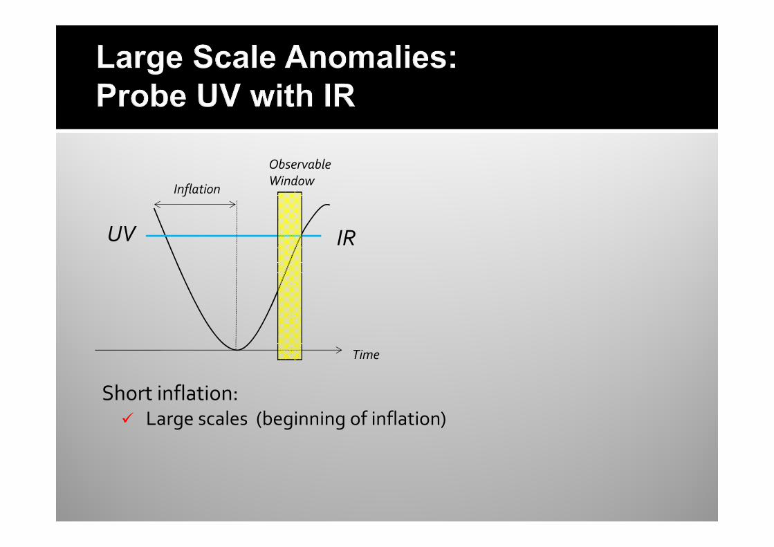
IR
Inflation
Time
Observable
Window
UV
Short inflation:� Large scales (beginning of inflation)
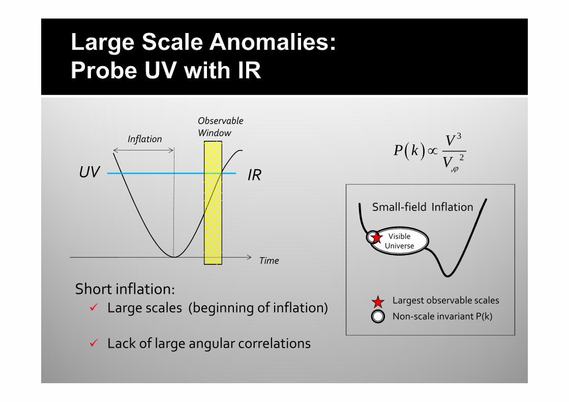
IR
Inflation
Time
Observable
Window
UV
Short inflation:� Large scales (beginning of inflation)
� Lack of large angular correlations
( )3
2,
VP k
Vϕ
∝
Largest observable scales
Non-scale invariant P(k)
Visible Universe
Small-field Inflation
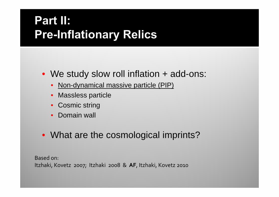
Based on:
Itzhaki, Kovetz 2007; Itzhaki 2008 & AF, Itzhaki, Kovetz 2010
• We study slow roll inflation + add-ons:• Non-dynamical massive particle (PIP)• Massless particle• Cosmic string• Domain wall
• What are the cosmological imprints?
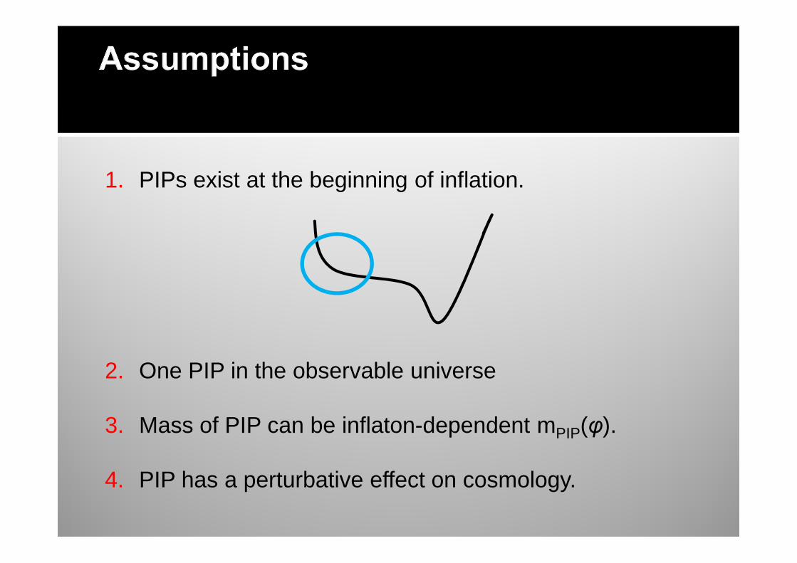
1. PIPs exist at the beginning of inflation.
2. One PIP in the observable universe
3. Mass of PIP can be inflaton-dependent mPIP(φ).
4. PIP has a perturbative effect on cosmology.
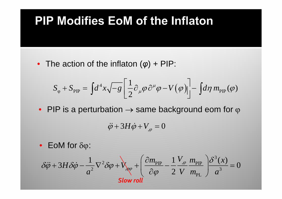
Slow roll
3,2 PIP PIP
,2 3PL
1 1 ( )3 0
2
Vm m xH V
a V m aϕ
ϕϕ
δδϕ δϕ δϕ
ϕ ∂
+ − ∇ + + − = ∂ && &
• The action of the inflaton (φ) + PIP:
( )4φ PIP PIP
1( )
2S S d x g V d mµ
µϕ ϕ ϕ η ϕ + = − ∂ ∂ − − ∫ ∫
,3 0H Vϕϕ ϕ+ + =&& &
• EoM for δϕ:
• PIP is a perturbation → same background eom for ϕ
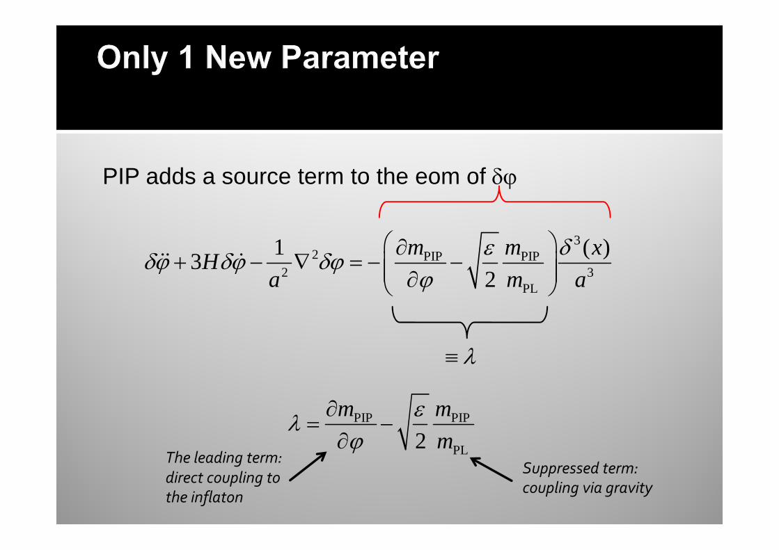
PIP adds a source term to the eom of δϕ
32 PIP PIP
2 3PL
1 ( )3
2
m m xH
a m a
ε δδϕ δϕ δϕ
ϕ
∂+ − ∇ = − − ∂
&& &
PIP PIP
PL2
m m
m
ελ
ϕ∂
= −∂
Suppressed term: coupling via gravity
The leading term:
direct coupling to the inflaton
λ≡
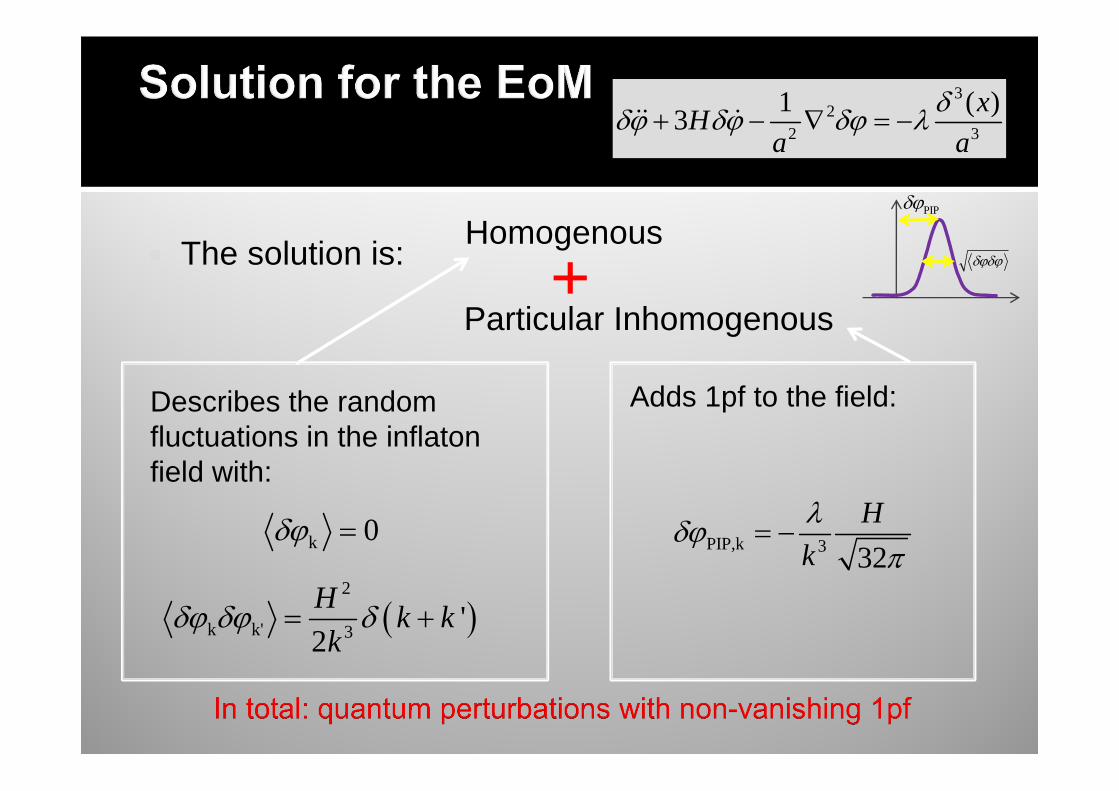
� The solution is:
32
2 3
1 ( )3
xH
a a
δδϕ δϕ δϕ λ+ − ∇ = −&& &
Homogenous
Particular Inhomogenous
Describes the random fluctuations in the inflaton field with:
( )2
k k' 3'
2
Hk k
kδϕ δϕ δ= +
k 0δϕ = PIP,k 3 32
H
k
λδϕ
π= −
Adds 1pf to the field:
PIPδϕ
δϕδϕ
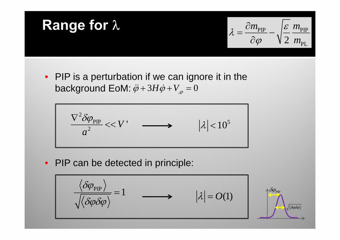
• PIP is a perturbation if we can ignore it in the background EoM:
• PIP can be detected in principle:
2PIP
2'V
a
δϕ∇<< 510λ <
PIP 1δϕ
δϕδϕ= (1)Oλ =
PIP PIP
PL2
m m
m
ελ
ϕ∂
= −∂
,3 0H Vϕϕ ϕ+ + =&& &
PIPδϕ
δϕδϕ
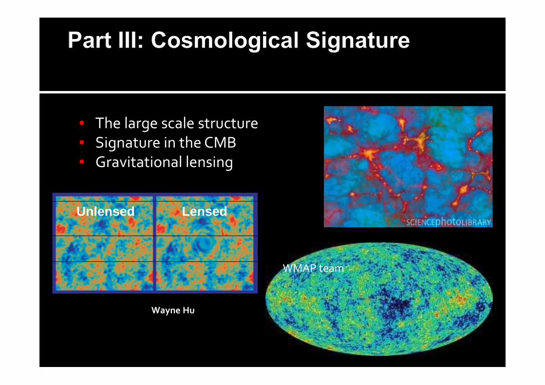
Wayne Hu
LensedUnlensed
WMAP team
• The large scale structure
• Signature in the CMB
• Gravitational lensing
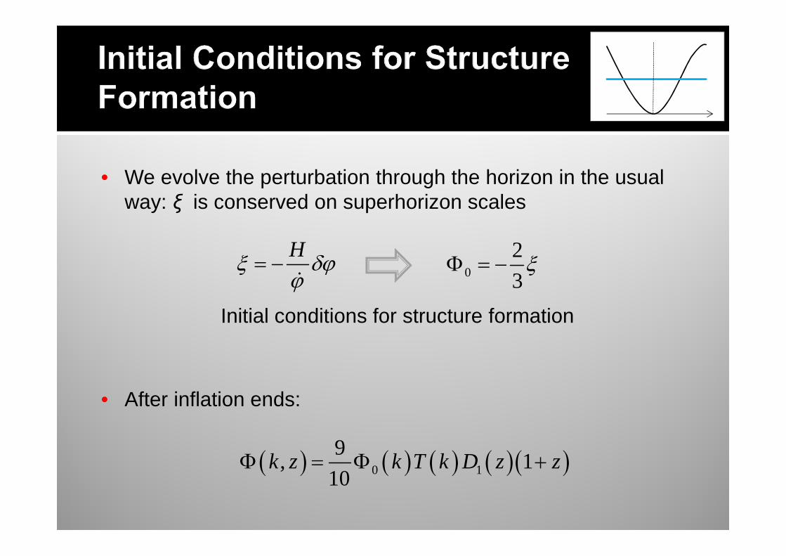
• We evolve the perturbation through the horizon in the usual way: ξ is conserved on superhorizon scales
• After inflation ends:
Hξ δϕ
ϕ= −
&0
2
3ξΦ = −
Initial conditions for structure formation
( ) ( ) ( ) ( ) ( )0 1
9, 1
10k z k T k D z zΦ = Φ +
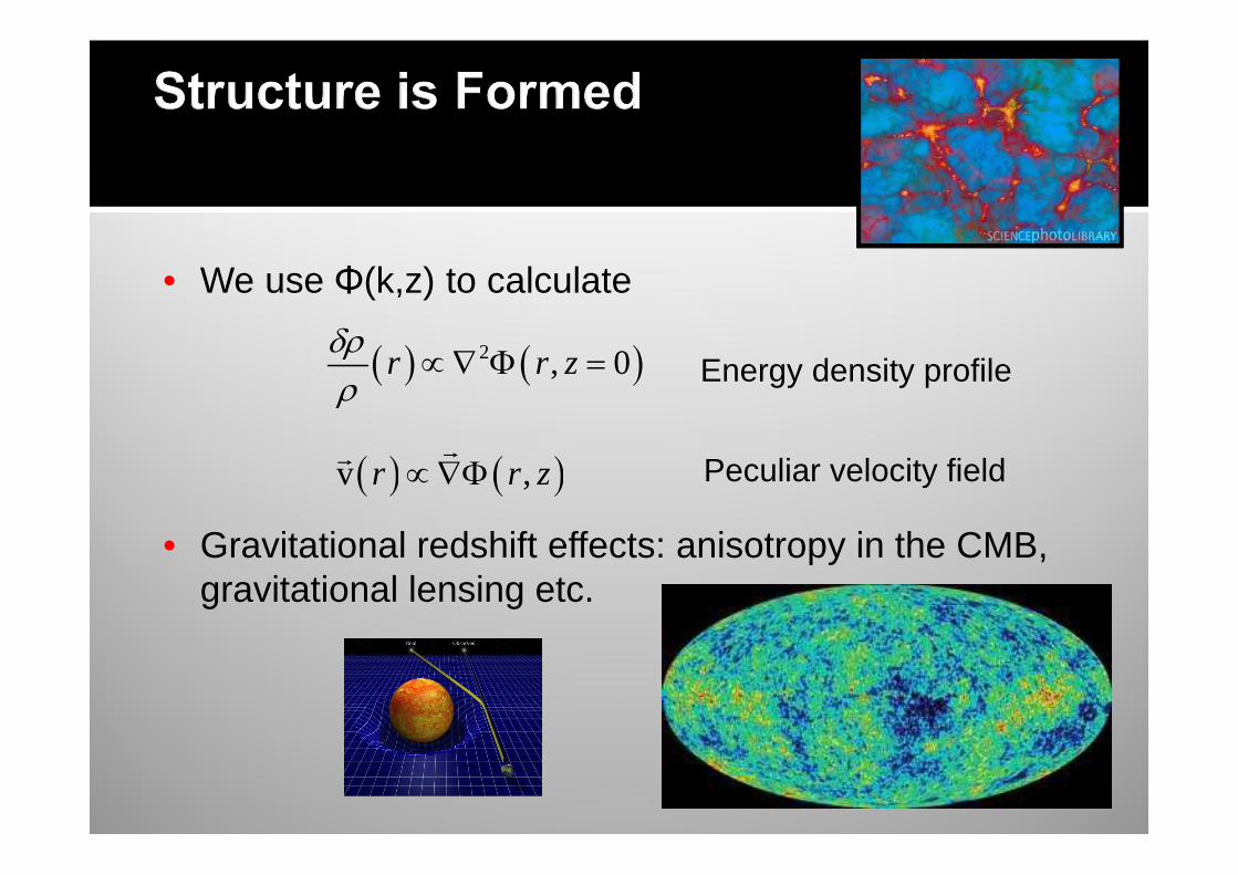
• We use Φ(k,z) to calculate
• Gravitational redshift effects: anisotropy in the CMB, gravitational lensing etc.
( ) ( )2 , 0r r zδρρ
∝∇ Φ = Energy density profile
( ) ( )v ,r r z∝∇Φrr
Peculiar velocity field
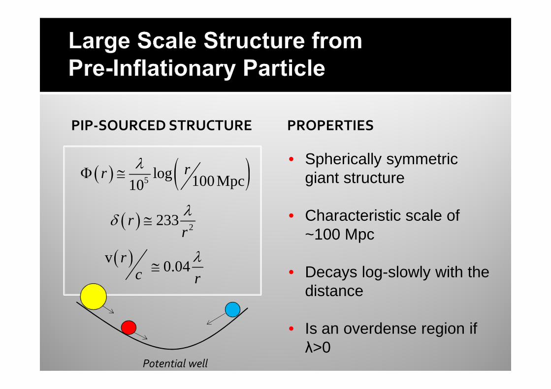
PIP-SOURCED STRUCTURE
• Spherically symmetric giant structure
• Characteristic scale of ~100 Mpc
• Decays log-slowly with the distance
• Is an overdense region if λ>0
PROPERTIES
( ) ( )5log 100Mpc10
rrλ
Φ ≅
( ) 2233r
r
λδ ≅
( )v0.04
rc r
λ≅
Potential well
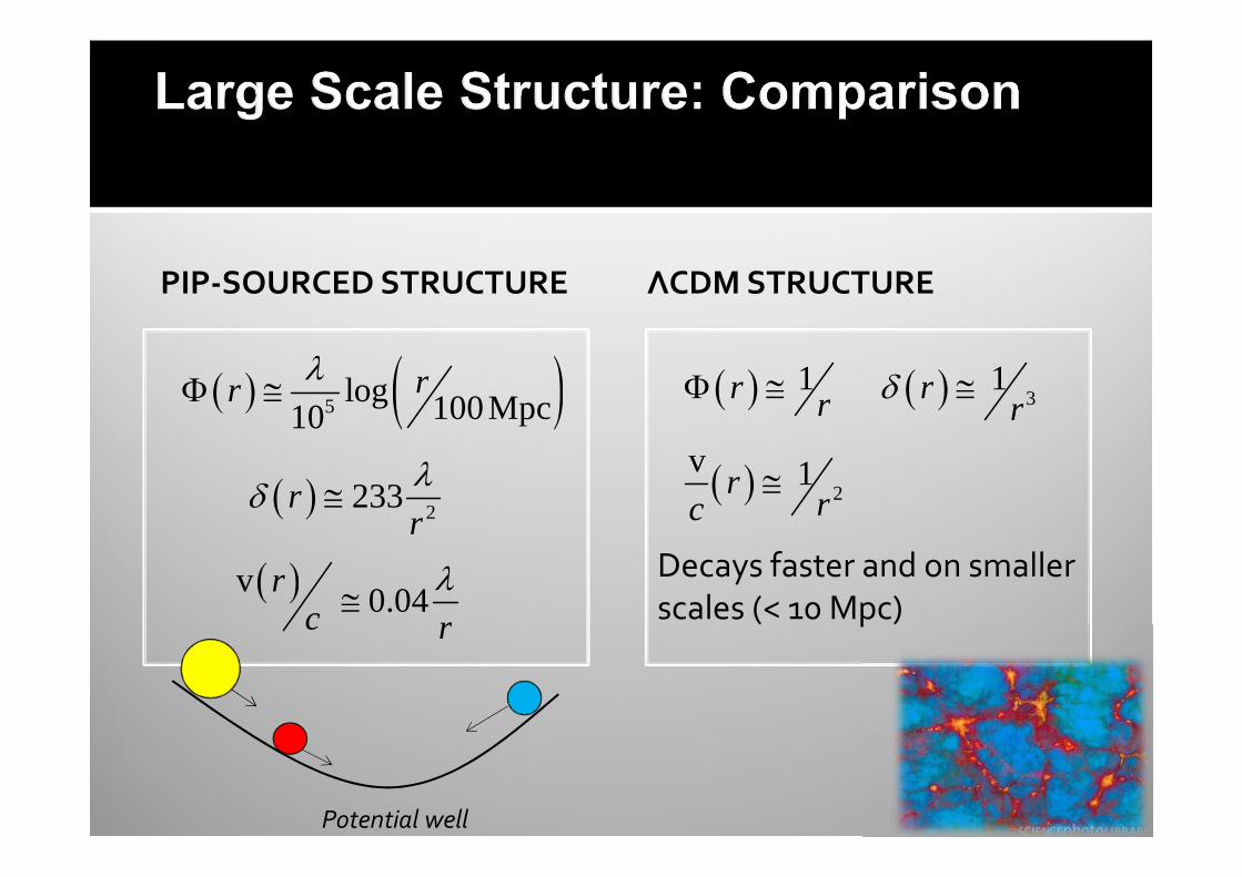
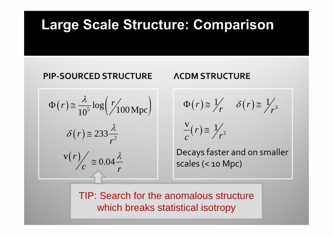
PIP-SOURCED STRUCTURE ΛCDM STRUCTURE
( ) ( )5log 100Mpc10
rrλ
Φ ≅
( ) 2233r
r
λδ ≅
( ) 1r rΦ ≅ ( ) 31r
rδ ≅
( ) 2
v 1rrc
≅
Potential well
Decays faster and on smaller
scales (< 10 Mpc)( )v
0.04r
c r
λ≅
PIP-SOURCED STRUCTURE ΛCDM STRUCTURE
( ) ( )5log 100Mpc10
rrλ
Φ ≅
( ) 2233r
r
λδ ≅
( ) 1r rΦ ≅ ( ) 31r
rδ ≅
( ) 2
v 1rrc
≅
Decays faster and on smaller
scales (< 10 Mpc)
TIP: Search for the anomalous structure which breaks statistical isotropy
( )v0.04
rc r
λ≅
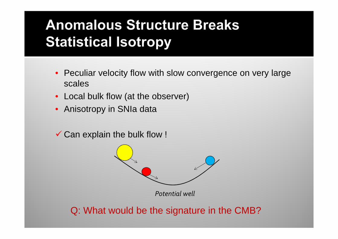
• Peculiar velocity flow with slow convergence on very large scales
• Local bulk flow (at the observer)• Anisotropy in SNIa data
� Can explain the bulk flow !
Q: What would be the signature in the CMB?
Potential well
Redshift
0
Observer
~1~1000
LSS
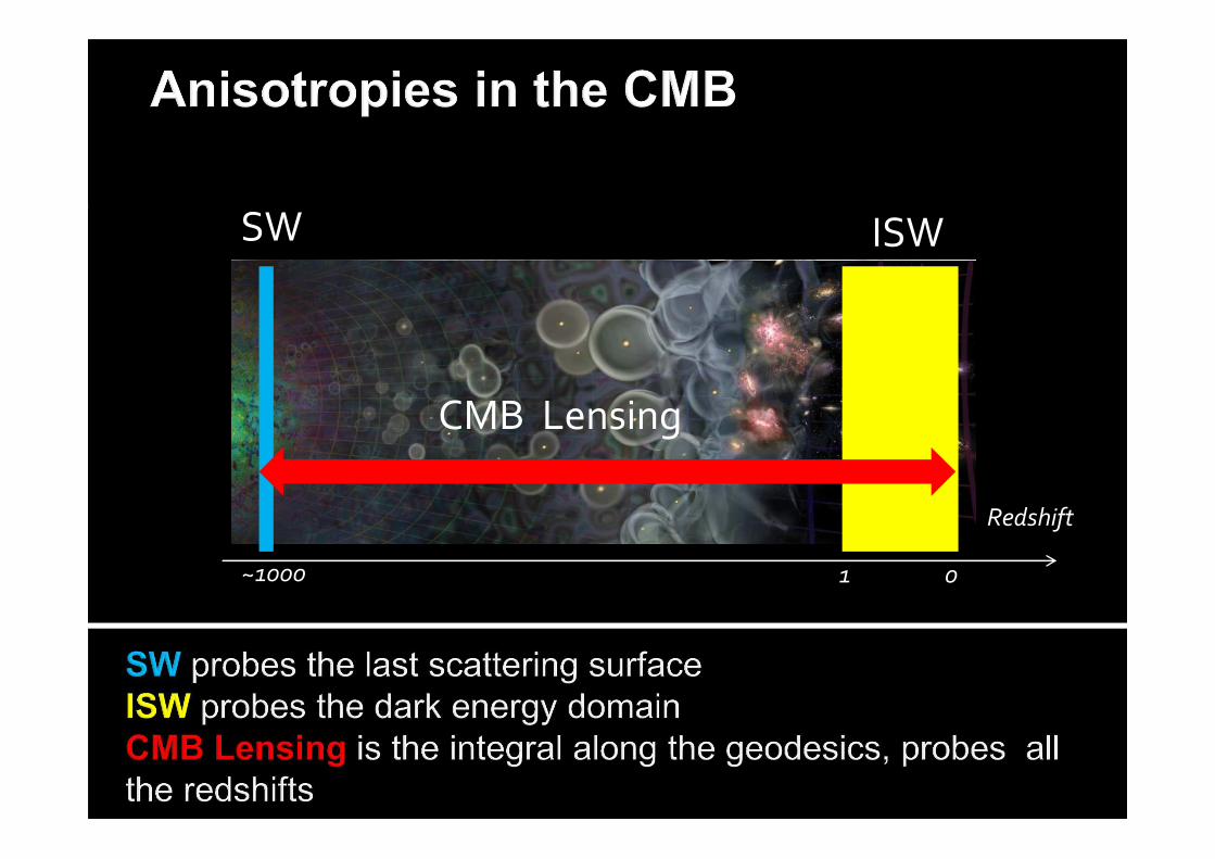
SW ISW
CMB Lensing
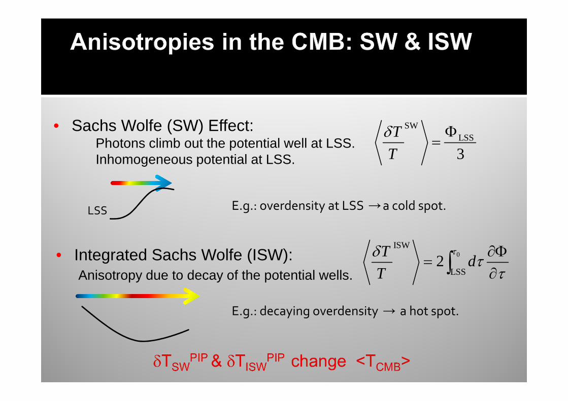
• Sachs Wolfe (SW) Effect:Photons climb out the potential well at LSS. Inhomogeneous potential at LSS.
LSS
SWLSS
3
T
T
δ Φ=
E.g.: overdensity at LSS /a cold spot.
• Integrated Sachs Wolfe (ISW): Anisotropy due to decay of the potential wells.
0ISW
LSS2
Td
T
τδτ
τ∂Φ
=∂∫
E.g.: decaying overdensity / a hot spot.
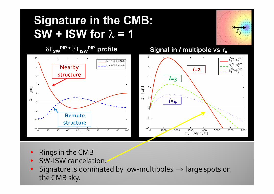
• Rings in the CMB• SW-ISW cancelation.• Signature is dominated by low-multipoles / large spots on
the CMB sky.
0r
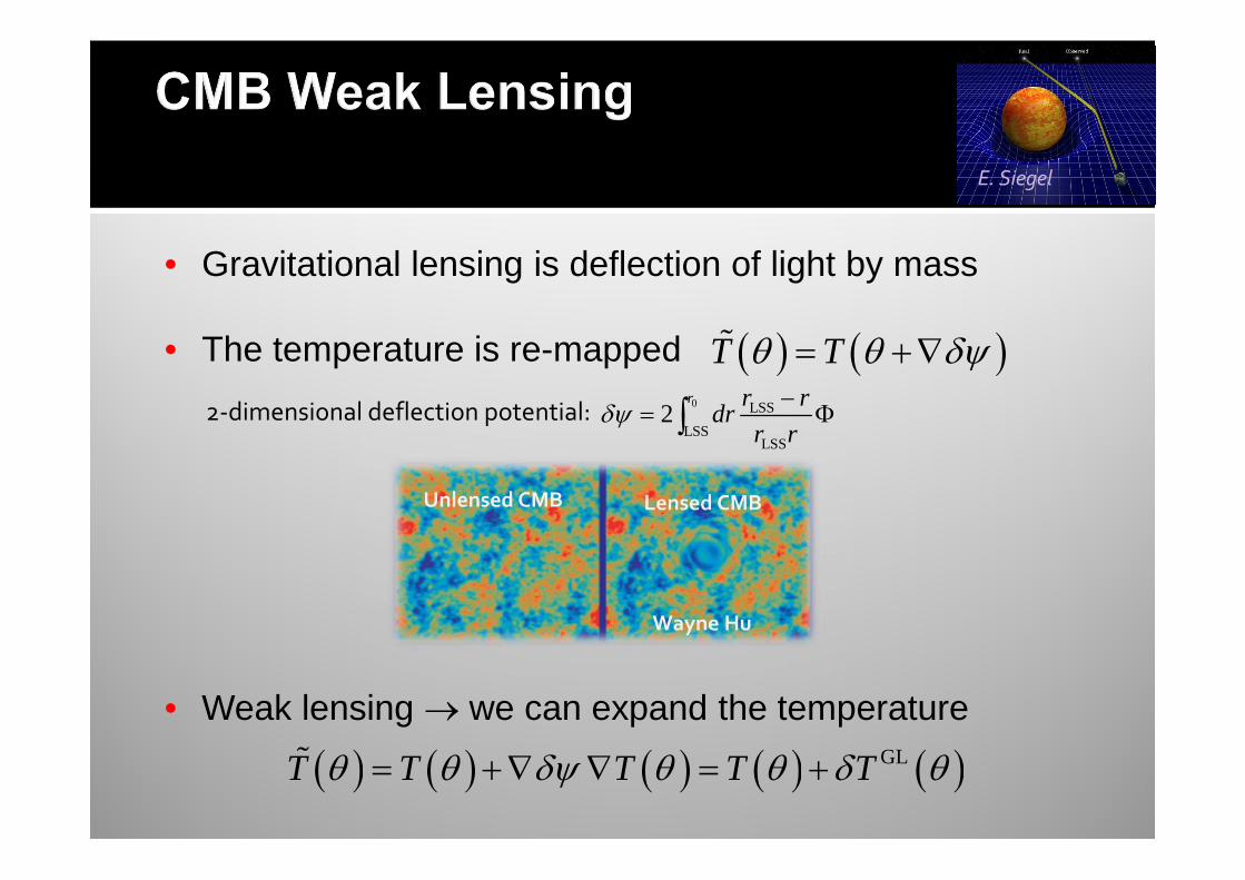
• Gravitational lensing is deflection of light by mass
• The temperature is re-mapped
• Weak lensing → we can expand the temperature
Wayne Hu
Lensed CMBUnlensed CMB
0 LSS
LSSLSS
2r r r
drr r
δψ−
= Φ∫
E. Siegel
( ) ( )T Tθ θ δψ= +∇%
2-dimensional deflection potential:
( ) ( ) ( ) ( ) ( )GLT T T T Tθ θ δψ θ θ δ θ= +∇ ∇ = +%
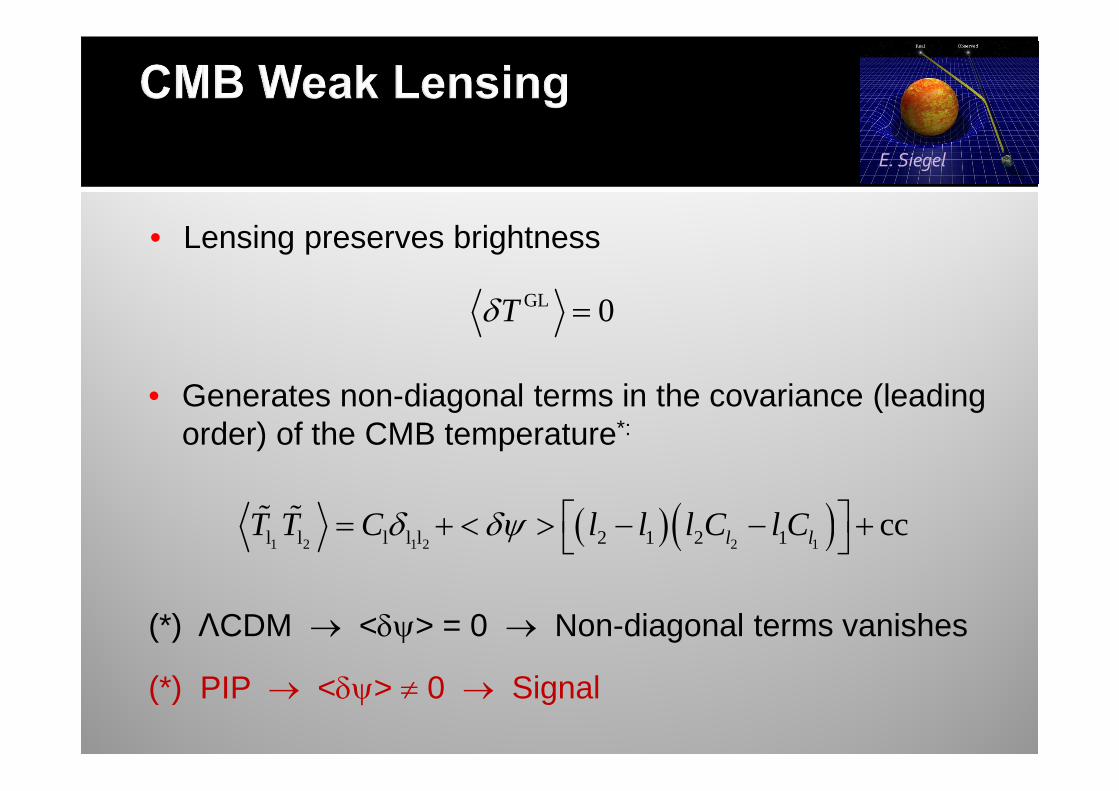
• Generates non-diagonal terms in the covariance (leading order) of the CMB temperature*:
(*) ΛCDM → <δψ> = 0 → Non-diagonal terms vanishes
(*) PIP → <δψ> ≠ 0 → Signal
E. Siegel
GL 0Tδ =
( ) ( )1 2 1 2 2 1l l l l l 2 1 2 1 ccl lT T C l l l C l Cδ δψ = + < > − − + % %
• Lensing preserves brightness
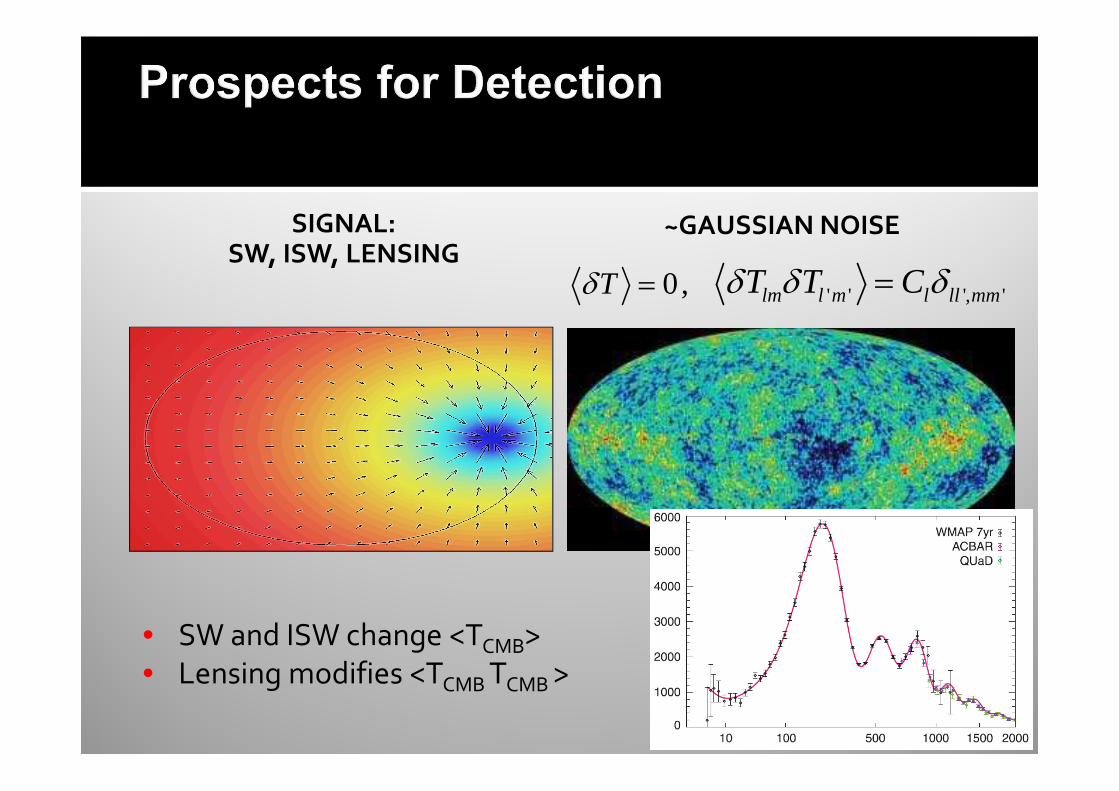
SIGNAL: SW, ISW, LENSING
~GAUSSIAN NOISE
0,Tδ = ' ' ', 'lm l m l ll mmT T Cδ δ δ=
• SW and ISW change <TCMB>
• Lensing modifies <TCMB TCMB >
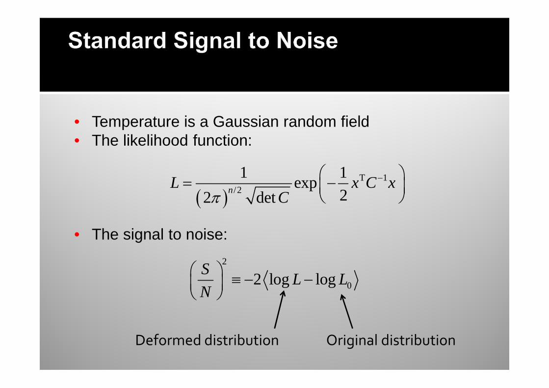
• Temperature is a Gaussian random field• The likelihood function:
• The signal to noise:
2
02 log logS
L LN
≡ − −
( )T 1
/2
1 1exp
22 detn
L x C xCπ
− = −
Deformed distribution Original distribution
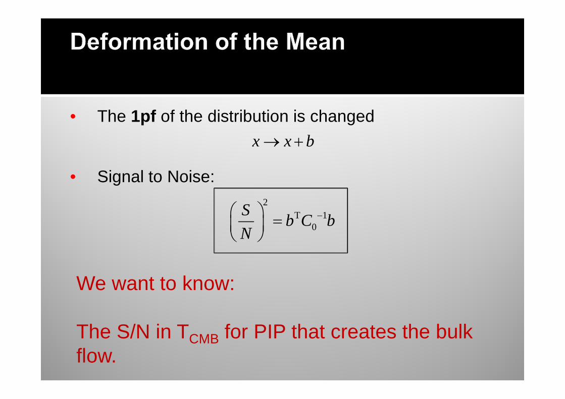
• The 1pf of the distribution is changed
• Signal to Noise:
x x b→ +
2T 1
0
Sb C b
N− =
We want to know:
The S/N in TCMB for PIP that creates the bulk flow.
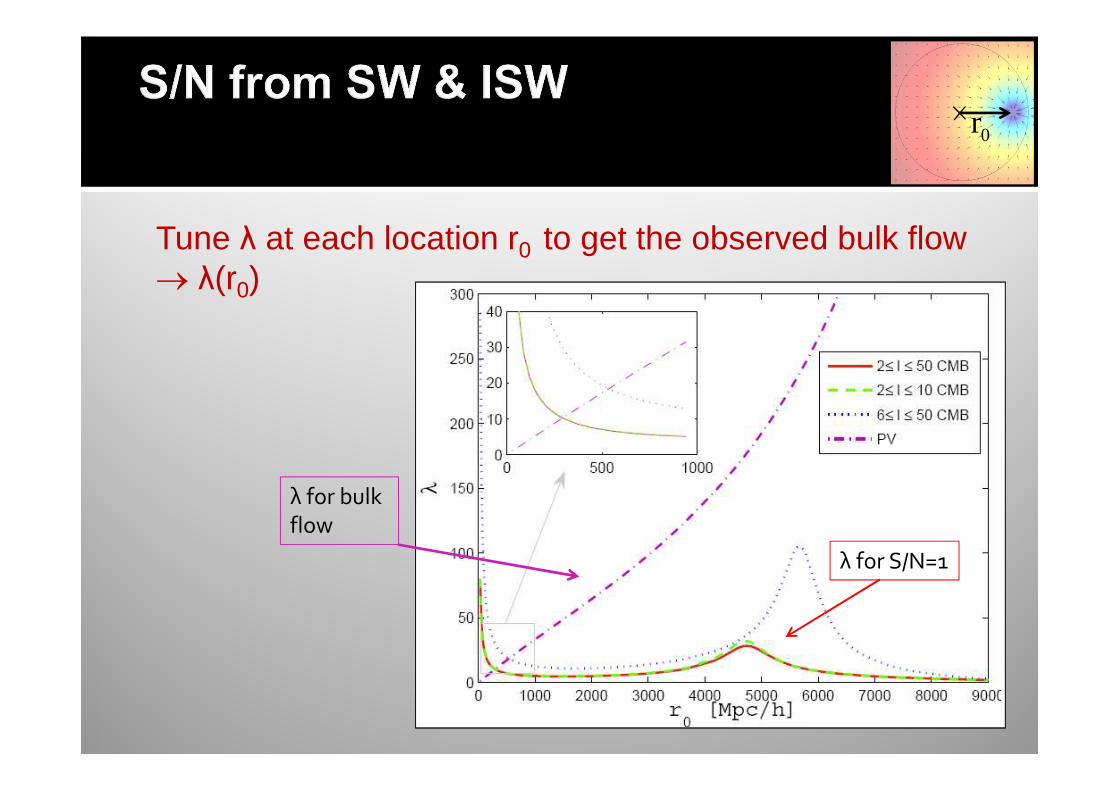
0r
λ for S/N=1
λ for bulk
flow
Tune λ at each location r0 to get the observed bulk flow → λ(r0)
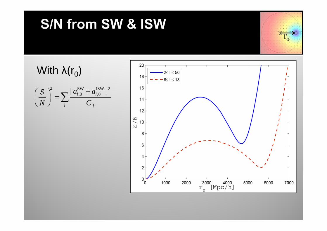
With λ(r0)
0r
2 SW ISW 2,0 ,0| |l l
l l
a aS
N C
+ =
∑
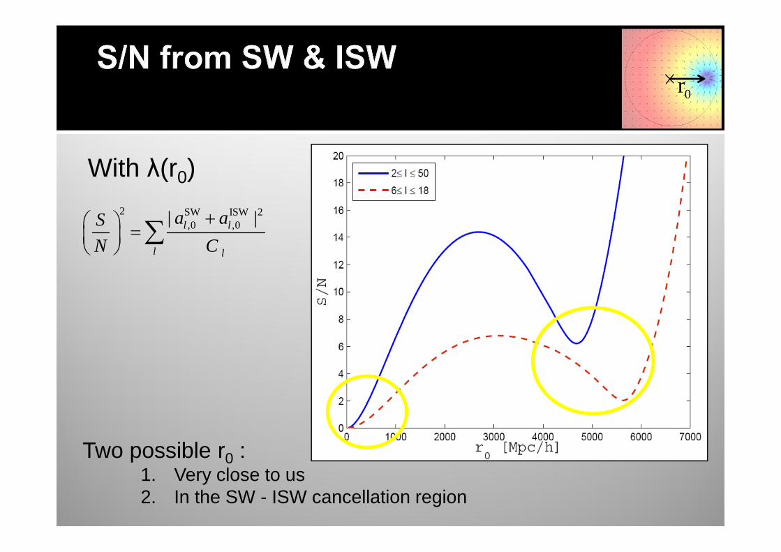
With λ(r0)
0r
Two possible r0 :1. Very close to us2. In the SW - ISW cancellation region
2 SW ISW 2,0 ,0| |l l
l l
a aS
N C
+ =
∑
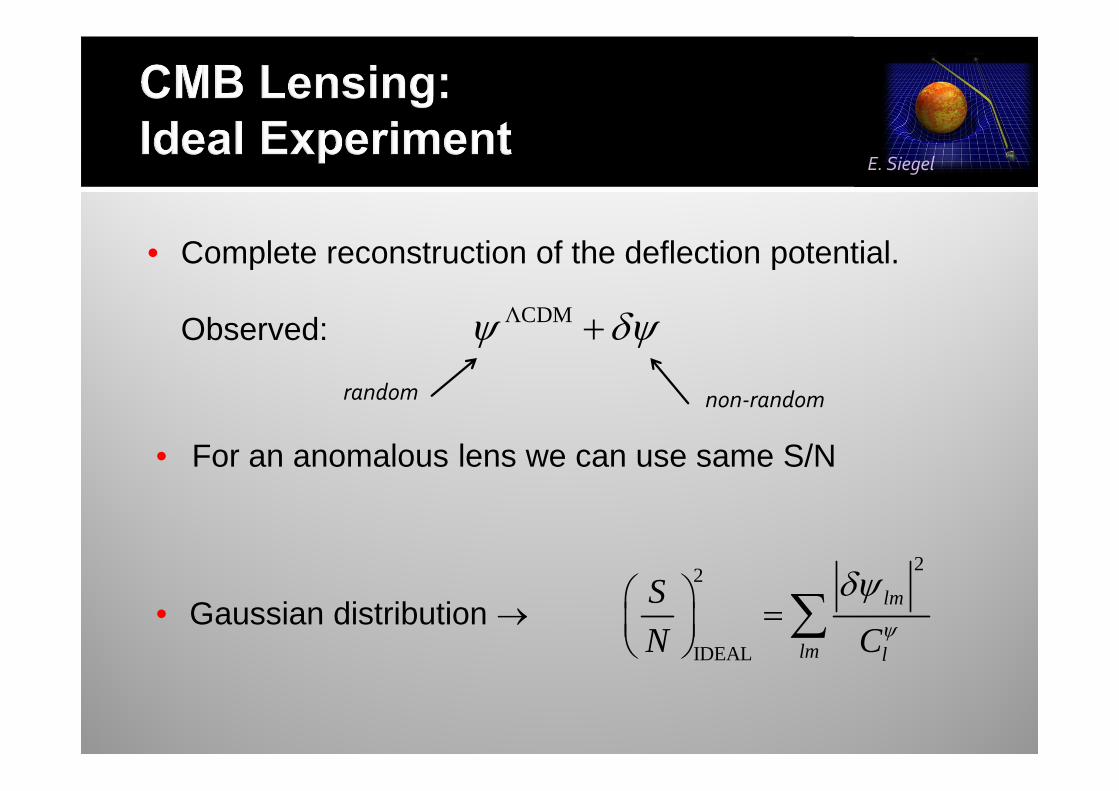
• For an anomalous lens we can use same S/N
• Complete reconstruction of the deflection potential.
Observed:
random non-random
ΛCDMψ δψ+
E. Siegel
• Gaussian distribution →
22
IDEAL
lm
lm l
S
N Cψ
δψ =
∑
E. Siegel
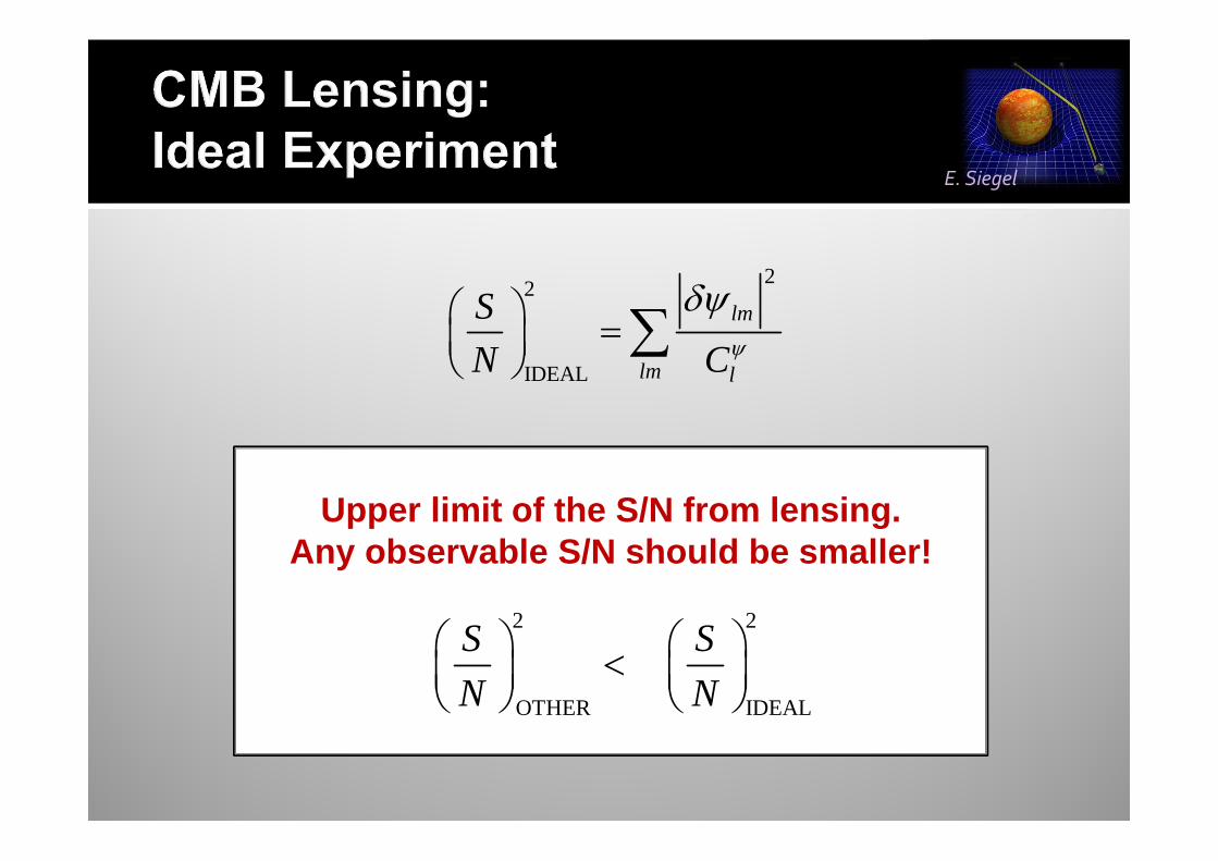
2 2
OTHER IDEAL
S S
N N <
Upper limit of the S/N from lensing. Any observable S/N should be smaller!
22
IDEAL
lm
lm l
S
N Cψ
δψ =
∑
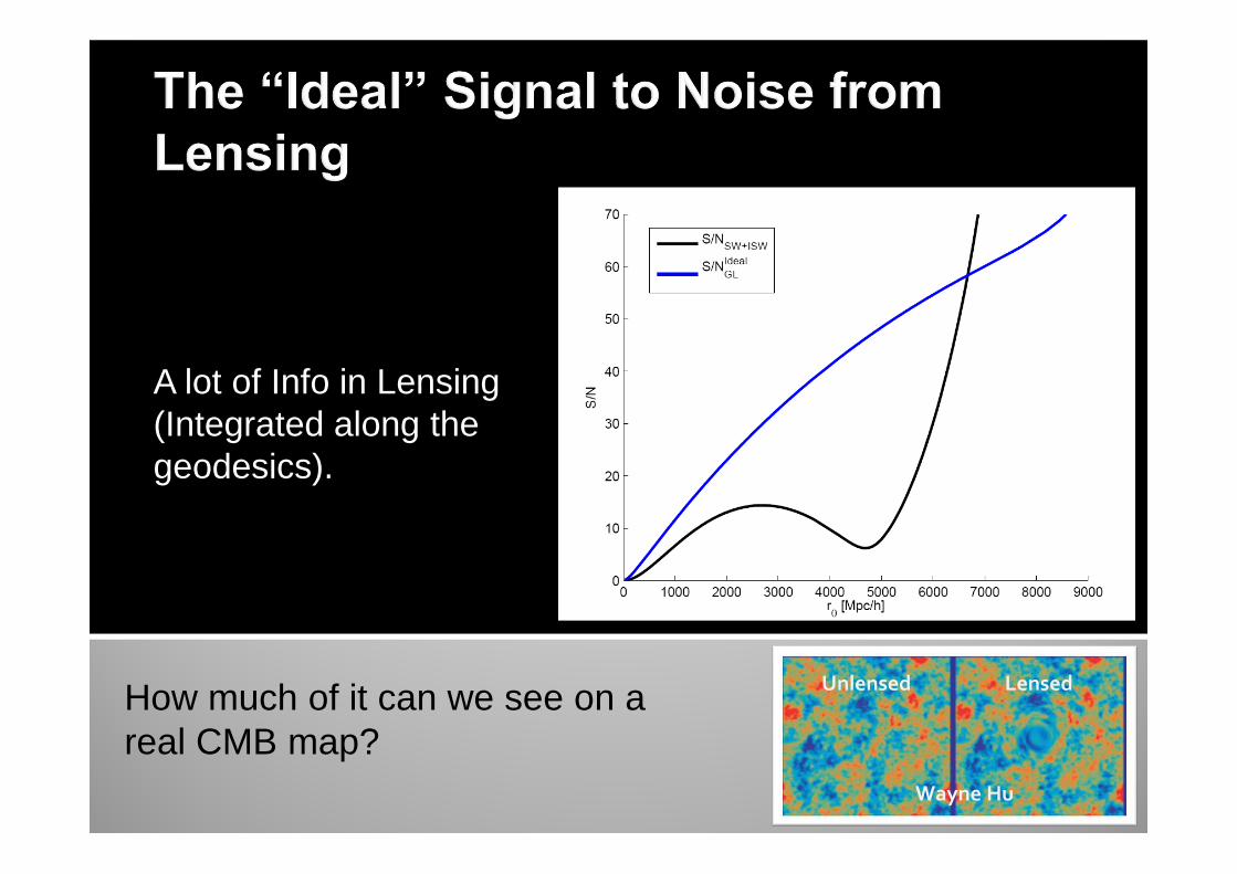
A lot of Info in Lensing (Integrated along the geodesics).
How much of it can we see on areal CMB map?
Wayne Hu
LensedUnlensed
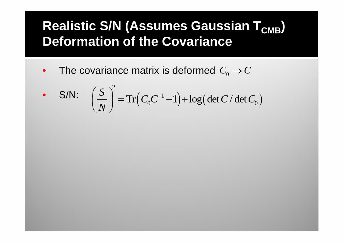
• The covariance matrix is deformed
• S/N:
0C C→
( ) ( )2
10 0Tr 1 log det / det
SC C C C
N− = − +
Realistic S/N (Assumes Gaussian TCMB)Deformation of the Covariance
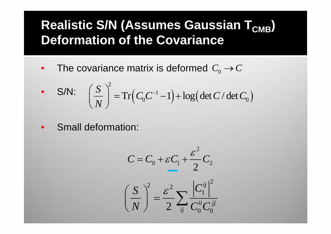
2
0 1 22C C C C
εε= + +
22 2
1
0 02
ij
ii jjij
CS
N C C
ε =
∑
• The covariance matrix is deformed
• S/N:
• Small deformation:
Realistic S/N (Assumes Gaussian TCMB)Deformation of the Covariance
0C C→
( ) ( )2
10 0Tr 1 log det / det
SC C C C
N− = − +
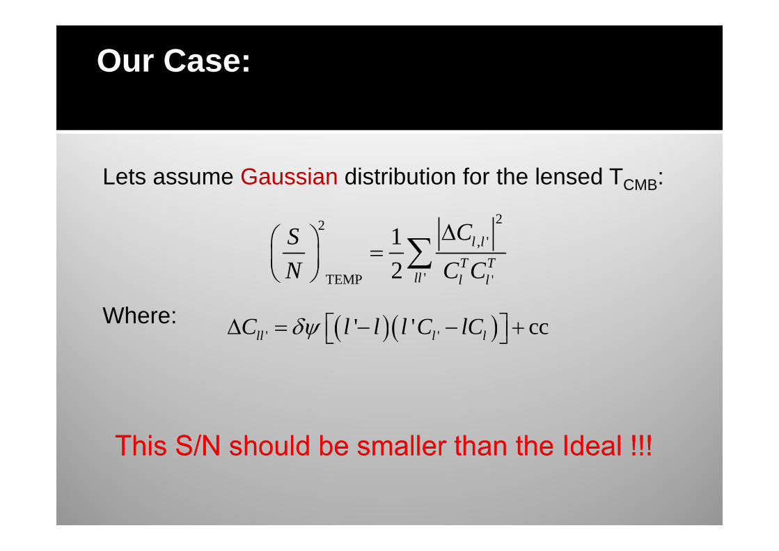
Lets assume Gaussian distribution for the lensed TCMB:
Where:
22, '
'TEMP '
1
2l l
T Tll l l
CS
N C C
∆ =
∑
( )( )' '' ' ccll l lC l l l C lCδψ∆ = − − +
Our Case:
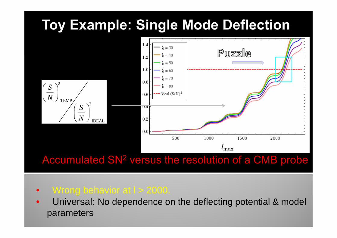
• Wrong behavior at l > 2000.• Universal: No dependence on the deflecting potential & model
parameters
2
TEMP2
IDEAL
S
NS
N
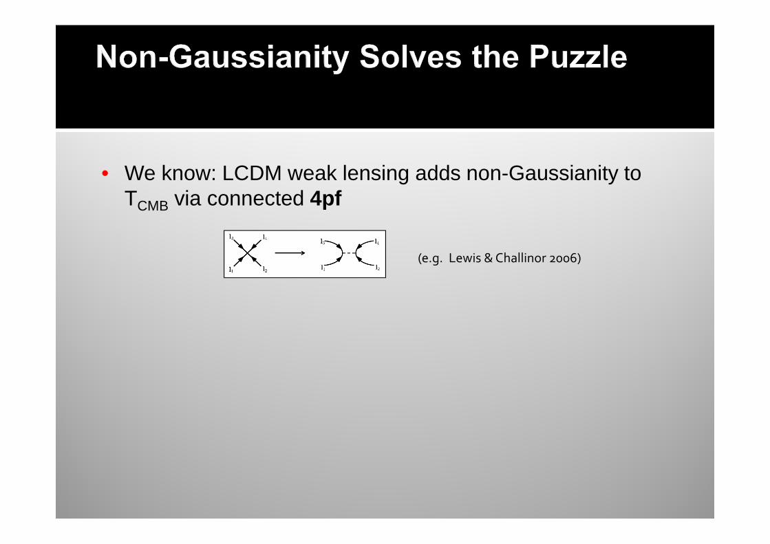
• We know: LCDM weak lensing adds non-Gaussianity to TCMB via connected 4pf
(e.g. Lewis & Challinor 2006)
(e.g. Lewis & Challinor 2006)
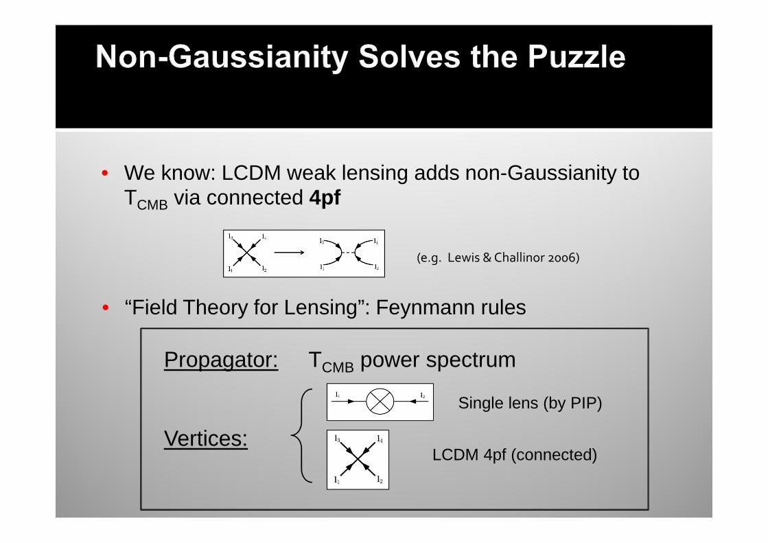
• “Field Theory for Lensing”: Feynmann rules
Propagator: TCMB power spectrum
Vertices:LCDM 4pf (connected)
Single lens (by PIP)
• We know: LCDM weak lensing adds non-Gaussianity to TCMB via connected 4pf
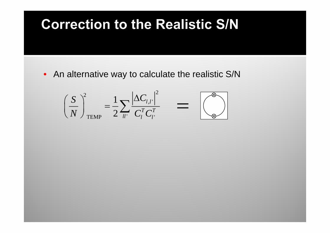
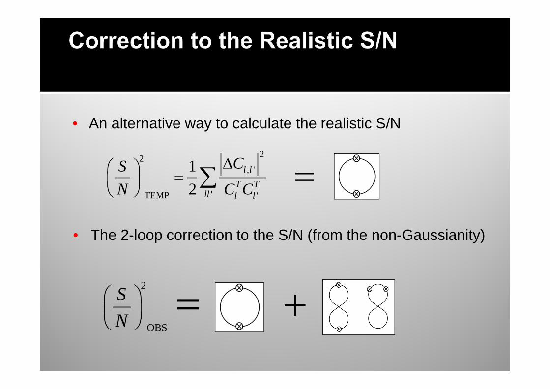
• An alternative way to calculate the realistic S/N
22, '
'TEMP '
1
2l l
T Tll l l
CS
N C C
∆ =
∑ =
22, '
'TEMP '
1
2l l
T Tll l l
CS
N C C
∆ =
∑ =
• The 2-loop correction to the S/N (from the non-Gaussianity)
+2
OBS
S
N
=
• An alternative way to calculate the realistic S/N
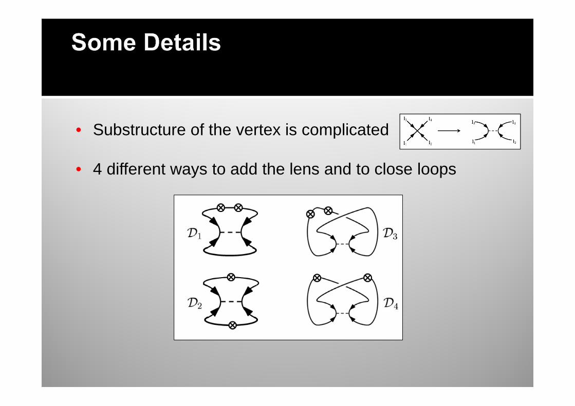
• Substructure of the vertex is complicated
• 4 different ways to add the lens and to close loops
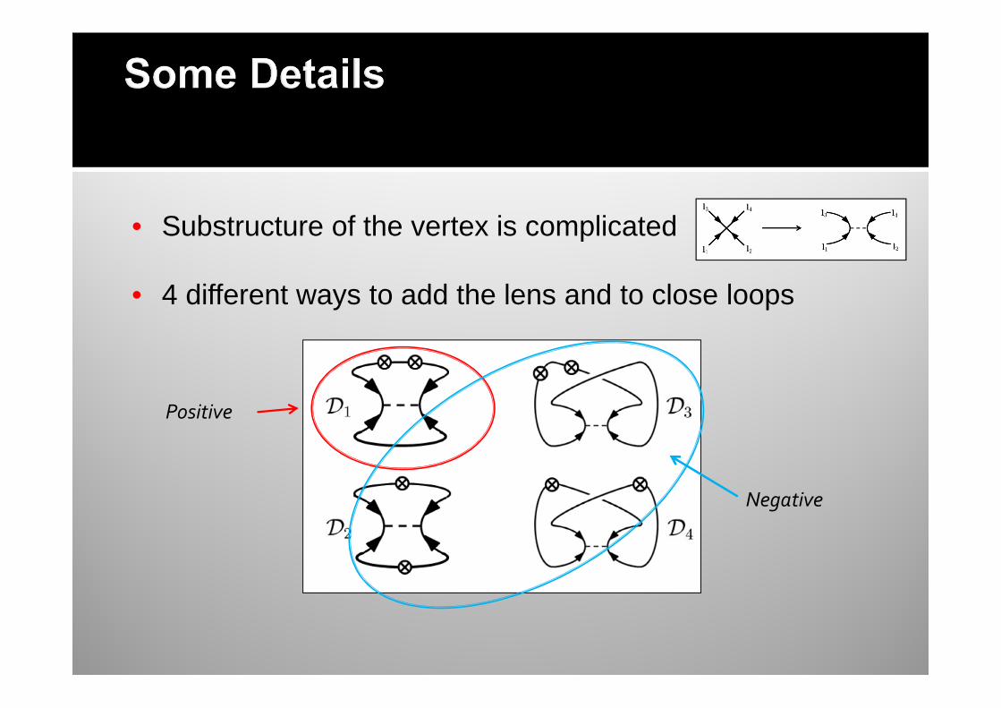
Positive
Negative
• Substructure of the vertex is complicated
• 4 different ways to add the lens and to close loops

( ) ( )2 2
OBS IDEAL
1
10S S
N N=
2
OBS2
IDEAL
S
NS
N
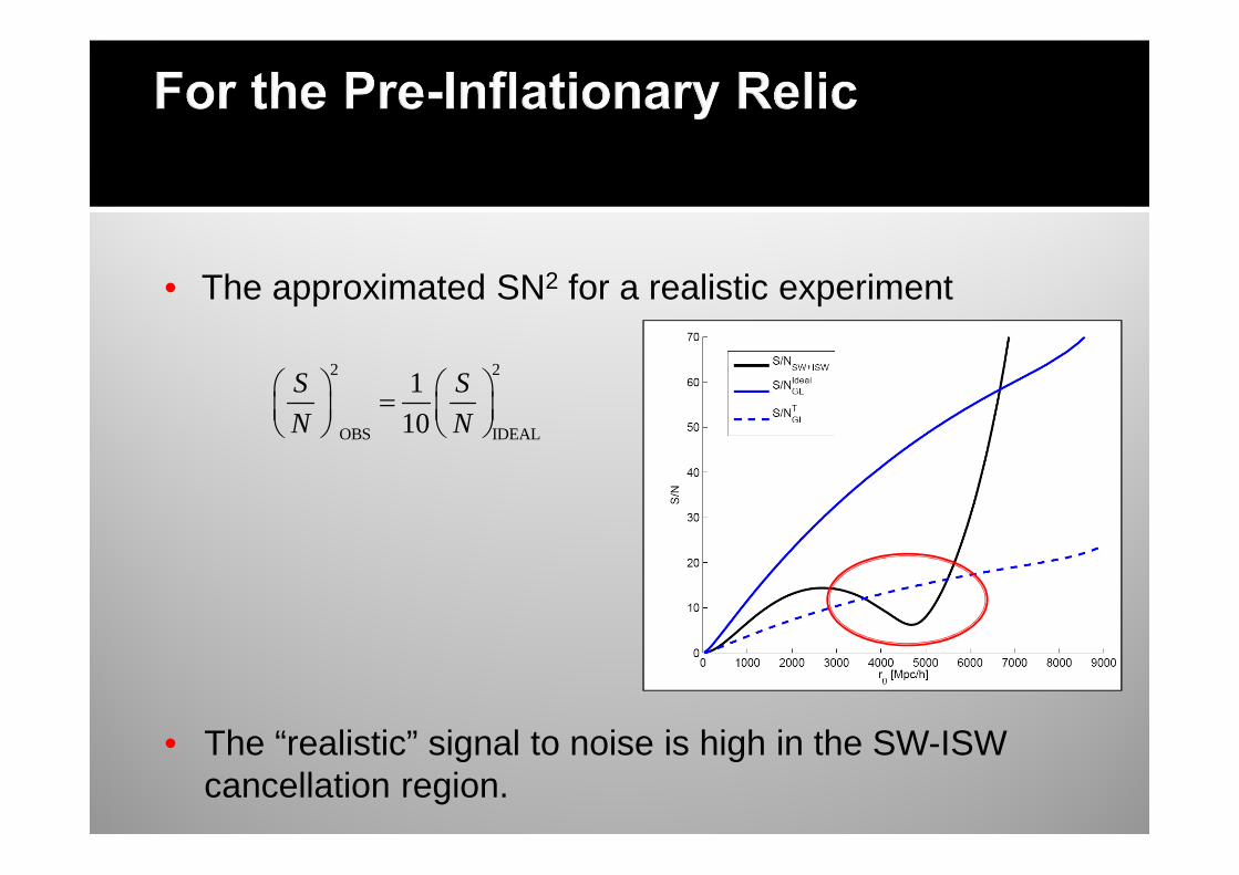
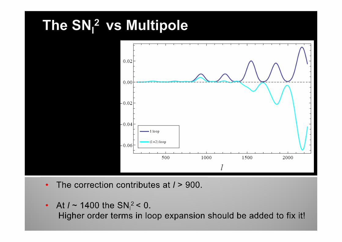
• The approximated SN2 for a realistic experiment
• The “realistic” signal to noise is high in the SW-ISW cancellation region.
2 2
OBS IDEAL
1
10
S S
N N =
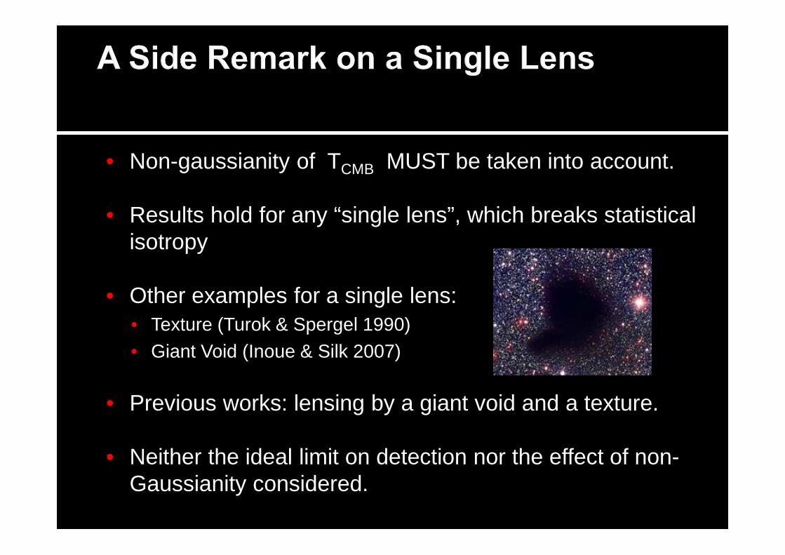
• Non-gaussianity of TCMB MUST be taken into account.
• Results hold for any “single lens”, which breaks statistical isotropy
• Other examples for a single lens:• Texture (Turok & Spergel 1990)• Giant Void (Inoue & Silk 2007)
• Previous works: lensing by a giant void and a texture.
• Neither the ideal limit on detection nor the effect of non-Gaussianity considered.
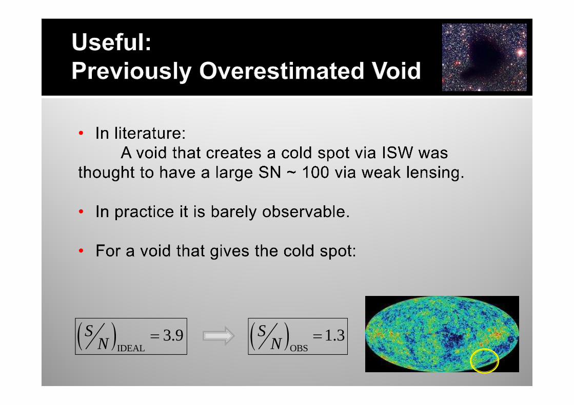
( )IDEAL
3.9SN = ( )
OBS1.3S
N =
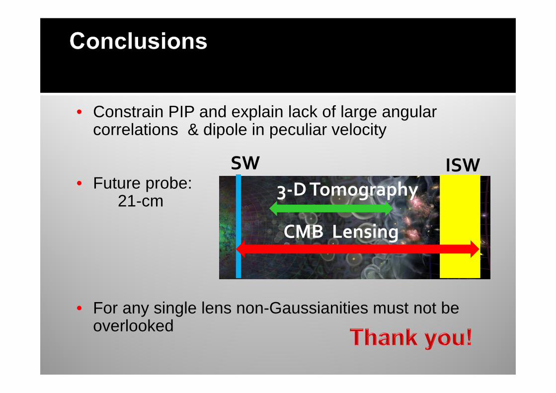
• Constrain PIP and explain lack of large angular correlations & dipole in peculiar velocity
• Future probe:21-cm
• For any single lens non-Gaussianities must not be overlooked
SW ISW
CMB Lensing
3-D Tomography