Analysis of the 0 Final States in COMPASS Data 1 Introduction This Bachelor’s thesis describes for...

Bachelor Thesis

Analysis of the η′π and ηπ Final States inCOMPASS Data

Christoph Raab

September 14, 2011

E

81

Physik Department E18Technische Universitat Munchen

Contents

1 Introduction 1

2 The COMPASS experiment 22.1 Purpose . . . . . . . . . . . . . . . . . . . . . . . . . . . . . . . . . . . . . 22.2 Design . . . . . . . . . . . . . . . . . . . . . . . . . . . . . . . . . . . . . . 22.3 Technical aspects of analysis . . . . . . . . . . . . . . . . . . . . . . . . . . 42.4 Motivation . . . . . . . . . . . . . . . . . . . . . . . . . . . . . . . . . . . 5

3 The η′π and ηπ final states 63.1 Properties and decay . . . . . . . . . . . . . . . . . . . . . . . . . . . . . . 63.2 Methods . . . . . . . . . . . . . . . . . . . . . . . . . . . . . . . . . . . . . 83.3 Preselection . . . . . . . . . . . . . . . . . . . . . . . . . . . . . . . . . . . 11

3.3.1 Preselection, first stage . . . . . . . . . . . . . . . . . . . . . . . . 113.3.2 Preselection, second stage . . . . . . . . . . . . . . . . . . . . . . . 193.3.3 Summary . . . . . . . . . . . . . . . . . . . . . . . . . . . . . . . . 21

3.4 Final Selection . . . . . . . . . . . . . . . . . . . . . . . . . . . . . . . . . 243.4.1 Second stage, channel ηπ− → (π+π0π−)π− . . . . . . . . . . . . . 243.4.2 Second stage, channel η′π− → (π+π−η)π− . . . . . . . . . . . . . . 253.4.3 Second stage, channel η′π− → (π+π−η(→ π+π0π−))π− . . . . . . 26

3.5 Conclusions . . . . . . . . . . . . . . . . . . . . . . . . . . . . . . . . . . . 303.6 Noted issues . . . . . . . . . . . . . . . . . . . . . . . . . . . . . . . . . . . 31

4 Acknowledgements 34

References 34

Bibliography 35

Chapter 1

Introduction

This Bachelor’s thesis describes for a large part the successful crosscheck of the selectionof the ηπ and η′π final states by Tobias Schluter that I performed from April 2011 upto early June 2011. As a result of this work, the analysis of Tobias Schluter could bepresented at the Hadron2011 conference in Munich. A similar analysis/crosscheck hadalready been performed by Tobias Schluter and Hauke Wohrmann.Theory has long predicted the existence of so-called exotic mesons which go beyond theconventional qq model. Their establishment and study is a subject of continued inter-est in the hadron physics community. One candidate for such an exotic meson is theπ1(1600), and one experiment with the versatility and precision to provide significantanalyses in the field of meson spectroscopy is COMPASS. The crosschecked event se-lection has the goal of isolating a specific state with as little background and as manyrepresantatives as possible. To this end, the selection criteria applied to a very largesample of events, the COMPASS 2008 hadron run, grow from general requirements onthe quality of the event to the identification of a specific decay chain.

1

Chapter 2

The COMPASS experiment

2.1 Purpose

The COMPASS (COmmon Muon and Proton Apparatus for Structure and Spectroscoy)experiment is a fixed-target experiment at the CERN North Area. Historically, it wascreated as a merger of two seperate proposals (HMC and Cheops) and thus serves abroad scientific programme and involves scientists of many institutions. The followingsection will describe the experimental setup that was used taking the data that areanalysed in this thesis, which is the hadron beam setup from 2008.

2.2 Design

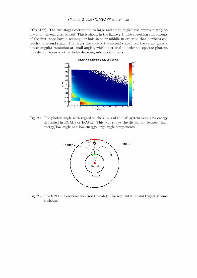
The COMPASS experiment is positioned at the end of the M2 beamline fed by the Su-per Proton Synchrotron (SPS). As illustrated in figure 2.4, the proton beam is directedinto a Beryllium production target. This produces predominantly pions, secondary pro-tons and a certain percentage of kaons. The M2 beamline guides the beam from theunderground level of SPS to the surface level of COMPASS. The two bending magnetsused for this also act as a momentum filter. The length of the beamline allows for theformation of a tertiary muon beam from the decay π → µνµ, which can then be selectedby the afforementioned bending magnets. As shown in figure 2.3, CErenkov Differentialcounters with Acromatic Ring focus (CEDARs) are set in place to identify the variousbeam particles. Other detectors placed upstream from the target are several triggerdetectors and the silicon telescope, which measures the beam direction. The target itselfis a barrel of liquid H2. It is surrounded by a Recoil Proton Detector (RPD) whichconsists of two rings. The inner ring A is 500 mm long and segmented into 12 slats ofscintillating polyvinyl toluoene (PVT) with a PMT (photo-multiplying tube) at eachend, the outer ring B is longer (1150 mm) and split into 24 slats. Please see the figure2.2 for an illustration. This design results in an azimuthal angular resolution of π

12 bycoinciding a slat in the inner ring with either one of the three slats in ring B which arefacing it. This scheme is shown in the cross section of figure 2.2, as well. The 655 mmradial separation of the between the rings allows for a measurement of the proton veloc-ity via its time of flight.

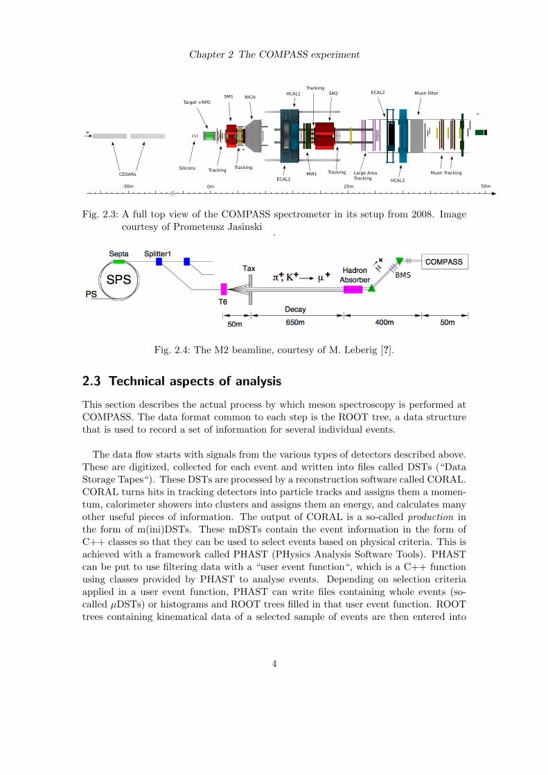
The subsequent spectrometer consists of two stages, each with a spectrometer magnetSM1/2, tracking detectors and hadronic and electromagnetic calorimetry (HCAL1/2,

2

Chapter 2 The COMPASS experiment

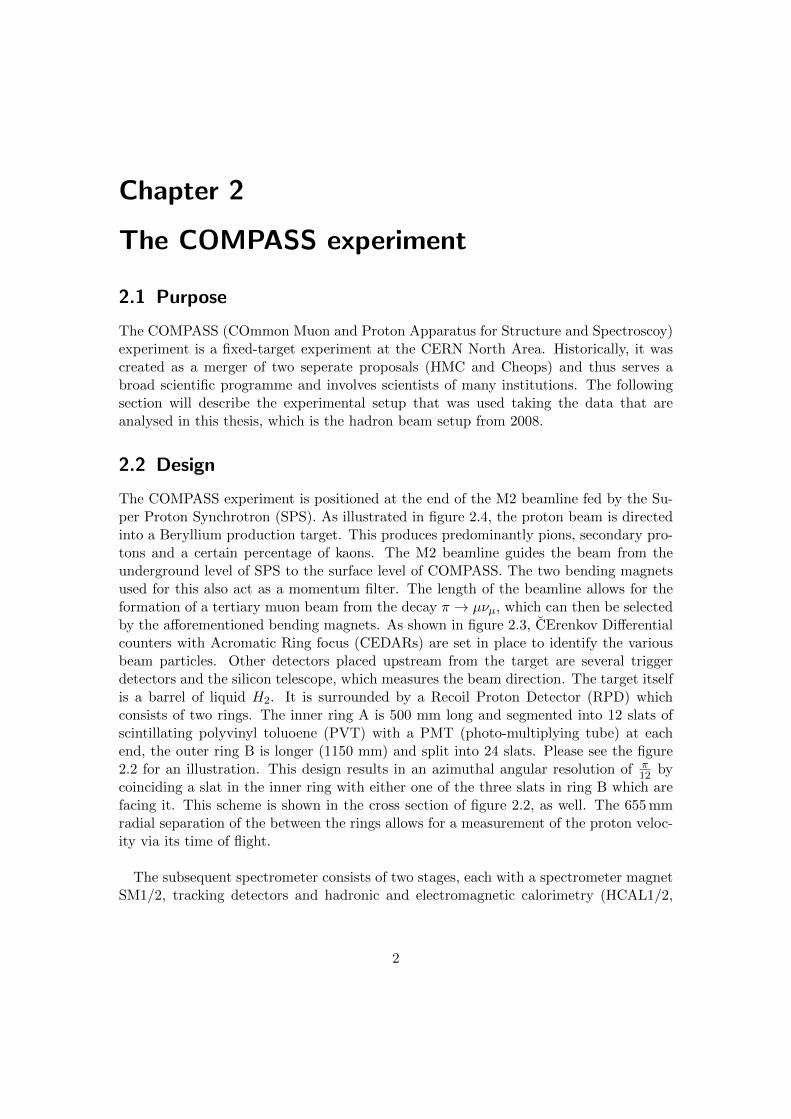
ECAL1/2). The two stages correspond to large and small angles and approximately tolow and high energies, as well. This is shown in the figure 2.1. The absorbing componentsof the first stage have a rectangular hole in their middle in order so that particles canreach the second stage. The larger distance of the second stage from the target gives abetter angular resolution at small angles, which is critical in order to separate photonsin order to reconstruct particles decaying into photon pairs.

Fig. 2.1: The photon angle with regard to the z axis of the lab system versus its energydeposited in ECAL1 or ECAL2. This plot shows the distinction between highenergy/low angle and low energy/large angle components.

Fig. 2.2: The RPD in a cross section (not to scale). The segmentation and trigger schemeis shown.

3


CEDARsSilicons

Target +RPDSM1

TrackingTracking

RICHHCAL1

TrackingSM2

ECAL1MW1 Tracking Large Area

Tracking HCAL2

ECAL2 Muon Filter

Muon Tracking

π

0m 50m25m-30m

Fig. 2.3: A full top view of the COMPASS spectrometer in its setup from 2008. Imagecourtesy of Prometeusz Jasinski

.

Fig. 2.4: The M2 beamline, courtesy of M. Leberig [?].

2.3 Technical aspects of analysis

This section describes the actual process by which meson spectroscopy is performed atCOMPASS. The data format common to each step is the ROOT tree, a data structurethat is used to record a set of information for several individual events.

The data flow starts with signals from the various types of detectors described above.These are digitized, collected for each event and written into files called DSTs (“DataStorage Tapes“). These DSTs are processed by a reconstruction software called CORAL.CORAL turns hits in tracking detectors into particle tracks and assigns them a momen-tum, calorimeter showers into clusters and assigns them an energy, and calculates manyother useful pieces of information. The output of CORAL is a so-called production inthe form of m(ini)DSTs. These mDSTs contain the event information in the form ofC++ classes so that they can be used to select events based on physical criteria. This isachieved with a framework called PHAST (PHysics Analysis Software Tools). PHASTcan be put to use filtering data with a “user event function“, which is a C++ functionusing classes provided by PHAST to analyse events. Depending on selection criteriaapplied in a user event function, PHAST can write files containing whole events (so-called µDSTs) or histograms and ROOT trees filled in that user event function. ROOTtrees containing kinematical data of a selected sample of events are then entered into

4


partial-wave analysis. Using a detailed model of the detector, Monte Carlo simulationprovides acceptance correction.

The analysis presented in this thesis focuses on the step of event selection; reconstruc-tion and partial-wave analysis are beyond the scope of the limited time available for abachelor’s thesis.

2.4 Motivation

This section describes the physical background of the analysis, the underlying assump-tions about the described events as well as a motivation.

In the constituent quark model, a meson is a fermion-antifermion bound system con-sisting of a quark and antiquark. The quark/antiquark couple to a spin S = 0, 1 andcan carry an orbital angular momentum L between them. These two in turn coupleto the total spin J = |L− S| , . . . , L + S. Commonly used parities are: the parity Pwhich describes the eigenvalue of a state under the parity transformation, and which isconserved by the strong interaction; the C parity, which belongs to charge conjugationbut strictly speaking only has neutral particles as eigenstates; and the G parity, whichis defined as the C parity times a rotation around the y-axis in isospin space and iswell-defined for all mesons. In conventional terms, the C parity of a charged meson isunderstood as that of its neutral isospin partner. Using basic properties of fermionicsystems and the qq assumption, these parities can be calculated as

P = (−1)L+1 (2.1)

C = (−1)L+S (2.2)

G = (−1)IC = (−1)L+S+I (2.3)

These equations lead to a set of forbidden quantum numbers not attainable in theconstituent quark model, namely the sequence JPC = 0−−, 0+−, 1−+, 2+−, . . .

Quantum chromodynamics (QCD), the fundamental theory of the strong interaction,predicts the existence of so-called exotic mesons beyond the constituent quark model.Showing the existence of these exotic mesons is a major goal in hadron physics. Dueto their exotic nature, their quantum numbers JPC are not restricted by the aboveequations. Thus, the preferred method of exotic meson searches is to show the existenceof “spin exotics“ with JPC quantum numbers impossible for pq mesons.

The π1(1600) is a candidate for such an exotic meson. It has been predicted by latticeQCD simulations as a hybrid meson with a mass below 2 GeV/c2[1]. Since, a numberof experiments claim a discovery of the π1(1600) with the spin-exotic quantum numbersJPC = 1−+ using various production mechanisms and decay modes. However, alongwith these individual analyses the state of establishment of the π1(1600) as a resonanceremains controversial. The COMPASS experiment provides new opportunities in thisregard with its capability of analysing many different decay modes.

5

Chapter 3

The η′π and ηπ final states

3.1 Properties and decay

After scattering on a proton, the beam particle diffracts into a state X while the protonstays intact. X decays into a final state at the “primary vertex”. The two final stateschosen for this analysis are ηπ− and η′π−. In other words, events need to be selectedwhich fit the reaction

π− + p→ X− + p→ η(′)π− + p (3.1)

To this end, the decays of these final states need to be reconstructed. The decay occursin a cascade of intermediate states, resulting in a system of particles which can beconsidered stable in the context of this experiment. In order to establish this distinction,we calculate the distance a particle might travel before it decays. This distance of coursedepends on the velocities β and life times τ of the involved particles, or alternativelytheir energies, masses and decay widths.

d = γβcτ =

√(E

m

)2

− 1 · ~cΓ

(3.2)

Relativistic time dilatation enters in the form of the factor γ. With the beam energy ofE = 191 GeV as the largest possible energy and the width of the π0 of Γ = 7.8 eV/c2 asthe smallest decay width of an intermediate particle involved in the interesting events,the estimated separation between the start and finish of the decay cascade is d = 35.5µm.As this distance is far below the resolution achievable at the current state of detectortechnology, the interaction and each occurring decay is assumed to occur instantaneously,in a single point, henceforth called the primary vertex.

The particles in the stable states are π± and photons. The π± only decay via theweak interaction, giving them a considerable smaller decay width of 2.5 · 10−8 eV/c2.Using the lower end of the E(π±) spectrum of 2 GeV as a low estimate of the involvedenergy, the same calculation arrives at a decay length of d = 112 m. This is longer thanthe spectrometer itself, which ends 51 m from the target. The vast majority of π± eitherdo not decay in the spectrometer, the small fraction that does travels a long enoughdistance so that the reconstruction of their trajectory is not inhibited.Free photons arestable unless they convert in an electric field, such as that of a nucleus. Keeping this

6

Chapter 3 The η′π and ηπ final states

in mind, we follow the decay chains of the chosen final states until we arrive at a stateconsisting only of charged pions and photons.

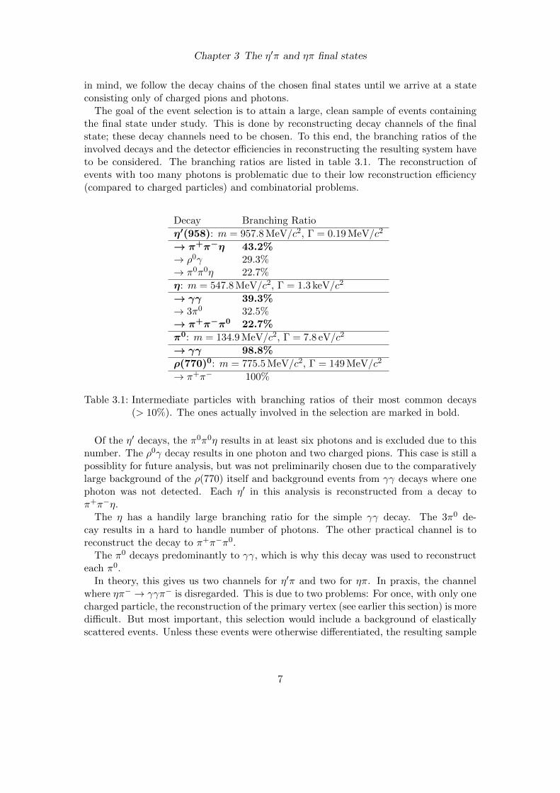
The goal of the event selection is to attain a large, clean sample of events containingthe final state under study. This is done by reconstructing decay channels of the finalstate; these decay channels need to be chosen. To this end, the branching ratios of theinvolved decays and the detector efficiencies in reconstructing the resulting system haveto be considered. The branching ratios are listed in table 3.1. The reconstruction ofevents with too many photons is problematic due to their low reconstruction efficiency(compared to charged particles) and combinatorial problems.

Decay Branching Ratio

η′(958): m = 957.8 MeV/c2, Γ = 0.19 MeV/c2

→ π+π−η 43.2%→ ρ0γ 29.3%→ π0π0η 22.7%

η: m = 547.8 MeV/c2, Γ = 1.3 keV/c2

→ γγ 39.3%→ 3π0 32.5%→ π+π−π0 22.7%

π0: m = 134.9 MeV/c2, Γ = 7.8 eV/c2

→ γγ 98.8%

ρ(770)0: m = 775.5 MeV/c2, Γ = 149 MeV/c2

→ π+π− 100%

Table 3.1: Intermediate particles with branching ratios of their most common decays(> 10%). The ones actually involved in the selection are marked in bold.

Of the η′ decays, the π0π0η results in at least six photons and is excluded due to thisnumber. The ρ0γ decay results in one photon and two charged pions. This case is still apossiblity for future analysis, but was not preliminarily chosen due to the comparativelylarge background of the ρ(770) itself and background events from γγ decays where onephoton was not detected. Each η′ in this analysis is reconstructed from a decay toπ+π−η.

The η has a handily large branching ratio for the simple γγ decay. The 3π0 de-cay results in a hard to handle number of photons. The other practical channel is toreconstruct the decay to π+π−π0.

The π0 decays predominantly to γγ, which is why this decay was used to reconstructeach π0.

In theory, this gives us two channels for η′π and two for ηπ. In praxis, the channelwhere ηπ− → γγπ− is disregarded. This is due to two problems: For once, with only onecharged particle, the reconstruction of the primary vertex (see earlier this section) is moredifficult. But most important, this selection would include a background of elasticallyscattered events. Unless these events were otherwise differentiated, the resulting sample

7


would have lower quality. Note that the BNL experiment E852 used this very channelin their analysis of the ηπ− final state [2].

In conclusion, the following decay chains are analysed:

X

X → ηπ−

η → π0π+π−

π0 → γγ

X → η′π−

η′ → ηπ+π−

η → γγ η → π0π+π−

π0 → γγ

Fig. 3.1: Summary of the analysed decay chains.

3.2 Methods

Kinematic fittingA constrained fit is a mathematical operation on a multi-dimensional fit parameter ya.Its objectiv is to find a variation ea so that it satisfies a constraint:

F (ya + ea) = 0 (3.3)

The variation ea is chosen so that the the error χ2 measured in the multi-dimensionalparameter space is minimal. To this end, a metric has to be introduced:

χ2 = eaC−1ab (ya)eb (3.4)

Mathematically, C is called the coveriance matrix. Its non-diagonal elements imply acorrelation between the parameters. This type of problem can be solved with standardmethods such as Lagrangian multiplicators. A kinematic fit such as the one applied inthis analysis is a type of constrained fit. Its constraint takes the form of

pµpµ −m2

0 = 0 (3.5)

That is, a four-momentum vector depending on fit parameters pµ(ya) has a certain in-variant mass m0. This can be motivated by the following application:

The η decays into two photons, which interact in the electromagnetic calorimeters ofCOMPASS and create two calorimeter showers, which are reconstructed as clusters withenergies E1,2 and positions ~x1,2. From these values, the four-momenta of the responsiblephotons can be reconstructed. Photons are massless and carry no charge. Assuminga photon being emitted at the primary vertex and depositing its whole energy in the

8


calorimeter, the four-momentum of the photon can be simply composed of the energyrecorded in the calorimeter cluster, scaled by a calibration factor, and the three-vectorwith the direction connecting the PV of the event to the location of the cluster and theenergy as its magnitude. The four-momenta of two photons reconstructed in this fashioncan then be added, the resulting invariant mass of two photons with the energies E1,2,with an angle θ between their momenta is then

m(γγ) = 2E1E2(1− cos θ) (3.6)

The energy resolution of the electromagnetic calorimeters is [7]

σ(E)

E=

5.5%√E⊕ 1.5% (3.7)

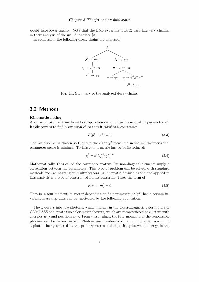
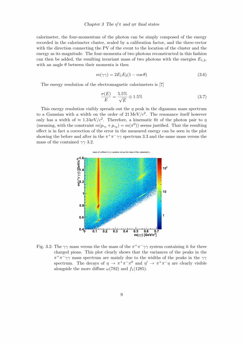
This energy resolution visibly spreads out the η peak in the digamma mass spectrumto a Gaussian with a width on the order of 21 MeV/c2. The resonance itself howeveronly has a width of ≈ 1.3 keV/c2. Therefore, a kinematic fit of the photon pair to η(meaning, with the constraint m(pγ1 +pγ2) = m(π0)) seems justified. That the resultingeffect is in fact a correction of the error in the measured energy can be seen in the plotshowing the before and after in the π+π−γγ spectrum 3.3 and the same mass versus themass of the contained γγ 3.2.

Fig. 3.2: The γγ mass versus the the mass of the π+π−γγ system containing it for threecharged pions. This plot clearly shows that the variances of the peaks in theπ+π−γγ mass spectrum are mainly due to the widths of the peaks in the γγspectrum. The decays of η → π+π−π0 and η′ → π+π−η are clearly visiblealongside the more diffuse ω(782) and f1(1285).

9


) [GeV]γγ-π+πm(0.8 0.9 1 1.1 1.2 1.3 1.4 1.5 1.6

even

ts/(

3 M

eV)

0

1

2

3

4

5

310× systemsγγ-π+πmass of unfitted

) [GeV]η-π+πm(0.8 0.9 1 1.1 1.2 1.3 1.4 1.5 1.6

even

ts/(

5 M

eV)

0

2

4

6

8

10

12

310×γγ fitted from η systems with an η-π+πmass

Fig. 3.3: For events with three charged pions, the effect of the kinematic fit of two pho-tons to the η mass is shown on the π+π−γγ spectrum. The kinematic fitsignificantly reduces the widths of both visible peaks belonging to the η′(985)and f1(1285). The results of the kinematic fit are listed in 3.2

Peak mass, width [ MeV/c2] η′(958) f1(1285)without kinematic fit m = 964.9, Γ = 23.6 m = 1287.9, Γ = 28.0with kinematic fit γγ to η m = 957.9, Γ = 5.4 m = 1280.8, Γ = 16.1PDG mass, partial width m = 957.8, Γ = 0.08 m = 1281.8, Γ = 12.6

Table 3.2: Results of the fit of the plots in 3.3. The peaks were fitted as Gaussians ontop of a linear background. The standard derivation is given as the width ofthe peak. The PDG widths are the partial widths for the relevant decays.Both peak positions are brought closer to the PDG masses, and both becomenarrower.

Such a kinematic fit was developed by Tobias Schluter and described in a COMPASSnote [4]. It features prominently in this analysis in three incarnations. All three have incommon that two calorimeter clusters are the only fit parameters involved. They differin their constraint. The simplest form is a constraint on the digamma mass, like in theexample above; it finds use in each of the chosen decay channels. Another one fits a sumof four-momenta including two photons to a mass, and is applied in the two channelswith three charged particles for both the ηπ− in section 3.4.1, and η′π− in section 3.4.2.The last one applies two constraints, one for the digamma mass and another one for theinvariant mass of a sum of four-momenta including two photons, and is applied as thelast step of the channel where η′π→5π±π0 3.4.3.

Cluster calibration

The calorimeter cells in the electromagnetic calorimeters in COMPASS exhibit re-sponses to photons which differ among them in their magnitude for the same energy ofa photon. The function deriving the energy of the photon which caused a calorimeter

10


shower from the signals of the cells involved in that shower therefore needs to contain ascaling factor for the energy deposited in each cell. That is

Ecalibrated = scaling(cell) · Euncalibrated (3.8)

In the data from production slot 3 available for this analysis, the π0 peak in the digammamass spectrum exhibited an offset from the PDG π0 mass, indicating a systematic errorin the current calibration. A preliminary calibration to mitigate this error was developedby Tobias Schluter [5].

The method proceeds this way:

1. A large sample of data is obtained where two calorimeter clusters have been mea-sured, and the resulting digamma mass lies within a window around the π0 mass.

2. Then, a kinematic fit (see the previous section 3.2) is performed to transform theenergies of these clusters.

3. The change in each cluster energy is then considered a scaling factor for the centralcell or cells of the clusters and averaged over the sample of events.

4. Using the already-obtained scaling factors, the process is then iterated.

In the production slot 4, a more advanced calibration which is currently being devel-oped by Sergei Gerassimov will be implemented, where the scaling factor can depend onthe cluster energy and time, as well.

3.3 Preselection

The cross-checked selection of the final states was performed in two stages. The first stage(section 3.3.1) was a pre-selection, part of a combined skim of the 2008 hadron mDSTsand used only basic cuts, trying to ensure clean, mostly exclusive events. The channel-specific selection was limited to the number of neutral clusters and charged tracks in theoutgoing system. Its goal was to reduce the data to a manageable amount, producing so-called µDSTs. The second stage started with another preselection (section 3.3.2) whichused said µDSTs as input and involved tighter and more advanced exclusivity cuts andkinematic fits. It then continued with the final selection (section 3.4), which identified therequired final states. Its end product were the trees entering into partial-wave analysis.

3.3.1 Preselection, first stage

DT0 trigger

The DT0 trigger is logically composed as aBT and RPD and not Veto, where aBT isthe alternative Beam Trigger, RPD the proton trigger and Veto a further composedsignal delivered by the veto system of COMPASS. Its purpose is to select an interactionbetween a beam particle and a target proton with a diffractively produced intermediary

11


state which decays inside the spectrometer’s acceptance, and it is commonly used in theCOMPASS 2008 hadron programme.In principle, it would be reasonable to require that the beam particle should be a π−

and not part of the 2.4% of K− in the beam. This percentage could be reduced in theselection to some degree by using the CEDAR particle identification detectors. As theirbehaviour is however not yet fully described in CORAL, this step was omitted.

Best primary vertex

The primary vertex (see section 3.1) is reconstructed as the the closest point of approachof the extrapolated beam and outgoing particle trajectories. The best primary vertex issuch a vertex that contains the highest number of exiting particle tracks.

At this stage, 14% of events contain no primary vertex, 80% contain exactly one andonly 5% contain more than one. As the best primary vertex is likely to be the physicalone, discounting 5% of events without further consideration does not seem justified.

Target cut

For the radius r and z coordinate of the primary vertex in the cylindrical lab system, itis demanded that

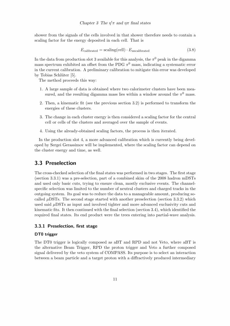
• −75 cm ≤ z(PV ) ≤ −25 cm

• r(PV ) ≤ 2.0 cm

A desired physical event describes the interaction of a beam pion inside the target ma-terial. On the other hand, all the material surrounding the liquid hydrogen of the target(the target container walls, parts of the spectrometer) can also give rise to an interac-tion producing several charged particles. The point of interaction is within reasonableerror the primary vertex (see 3.1), therefore the radial and z coordinates of the PV aresuitable to cut on the dimensions of cylindrical target container. In this step, the cutsare deliberately broad. They are tightened in the second stage of the selection in section3.3.2.

Number of charged particles

Since the intended selection includes either 3 or 5 charged pions, the number of chargedparticle tracks from the primary vertex is required to be ∈ {3, 4, 5}. The case of 4charged pions is excluded implicitly by the cut on the charge sum (see below).

Charge conservation

Assuming an elastic scattering π− + p → X− + p and subsequent decay of X− intothe outgoing system, the charge is conserved as the charge of the beam particle. Here,it is calculated as the sum of the charges of the charged particles exiting the primaryvertex. Assuming correct charge values for the individual particles, incorrect sums of the

12


Z [cm]-100 -80 -60 -40 -20 0

even

ts /

(0.4

cm

)

0

0.5

1

1.5

2

2.5

3

3.5

610×Z position of primary vertex

Fig. 3.4: The Z position of the primary vertex. The cut −75 cm ≤ Z(PV ) ≤ −25 cmapplied at this stage is marked and the length of the target is clearly visiblewithin this interval. The Z positions of silicon microstrip detectors withinthe RPD also appear as sources of primary vertices outside the target lengthinterval.

charges are due to charged particles which were missed by the detector or reconstructionsoftware. Such an event is obviously unfit for analysis. As is discussed in 3.6, for eachparticle track two methods exist in Phast to obtain the charge of the particle. Eventswhere one gave a correct and the other an incorrect value make up 0.01% of events. Inorder to ensure a good quality of this simple cut and in light of the minute loss in events,both were required to result in the correct sum, leaving 62% of events considered at thisstep.

Number of photons

The number of photons in the outgoing system is selected to be ∈ {2, 4, 6}. Each photonsupposed to hit a calorimeter and create an electromagnetic shower, resulting in a ”good”calorimeter cluster. Such a “good” cluster is defined by the following cuts:

• It has no charged particle tracks pointing towards it. This is required as chargedparticles like π± or e± from the conversion of a photon in a nuclear field γ → e+e−

also interact in the electromagnetic calorimeters.

• It occurs in either ECAL1 or ECAL2, which are the relevant calorimeters forphotons to deposit their energy into.

• It has a time associated with it which, relative to the mean time of the beamparticle, obeys −8 ns ≤ tcluster − tbeam ≤ 10 ns. In the range of of the z positiondistributions for clusters and primary vertices, the time for a photon to travel froma primary vertex within the target to an electromagnetic calorimeter can be foundto have an estimated variation of 3.5 ns for ECAL1 and 1.7 ns for ECAL2. This

13


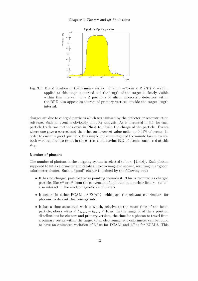
Fig. 3.5: The location of primary vertices in the x-y plane, shown in colour on a logarith-mic scale. The radial target cut is shown in white. Several features are clearlyvisible as illuminated by the beam: Moving from the inside out, the inner mostis the target material. The inhomogenous illumination by the pion beam isvisible with a centre at ≈ (0 cm, 0.4 cm) and an asymmetric extension to thelower right, while the level of the liquid hydrogen appears as a depleted areaat the top. The projection of the target container wall is visible as a ring ofradius ≈ 1.5 cm. In addition, hints of the target support structure and siliconmicrostrip detectors (see figure 3.4) appear.

variation, together with further errors in the time measurements, contributes tothe width of the main peak in the time spectra in figure 3.6. A cut on this mainpeak around t = 0 ns is used to reduce pileup events, i.e. events where particles inthe outgoing system are not all the result of the same primary interaction.

• The energy exceeds the lower bounds of E ≥ 1.0 for ECAL1 and E ≥ 4.0 forECAL2. These two energy thresholds are supposed to reduce noise introducedat low energies; however, the thresholds might still be too high. The variouscombinations of these thresholds are visible in the m(γγ) spectrum (figure 3.8).They do not seem to ingress into the two relevant peaks.

• In ECAL2, clusters within the cells obsured by the HCAL1 calorimeter are dis-carded. This limits their position to −17 · 3.83 cm ≤ ycluster ≤ 16 · 3.83 cm, where3.83 cm is the side length of a cell. The shadow of HCAL1 is treated as an exclusioncriterium as it was not yet considered in CORAL. In the digamma mass spectrumfor two photons in the outgoing system, the decays π0 → γγ and η → γγ are visibleas approximately Gaussian peaks on a background. Their shape is a result of the

14


[ns]beamt-t-40 -30 -20 -10 0 10 20 30 40

even

ts /

(250

ps)

410

510

610

710

Cluster time relative to beam for ECAL 1 in ns

[ns]beamt-t-40 -30 -20 -10 0 10 20 30 40

even

ts /

(250

ps)

310

410

510

610

710

Cluster time relative to beam for ECAL 2 in ns

Fig. 3.6: The time spectra for calorimeter clusters on a logarithmic scale, on the left forECAL1 and on the right for ECAL2. The cut made to select “good” clustersis marked.

uncertainty in the measured quantities; the natural partial width of these decaysis 7.7 eV/c2 for the π0 and 0.51 keV/c2 for the η, while using a fit to a Gaussianwith a linear background, the widths of the peaks can be estimated as 6 MeV/c2

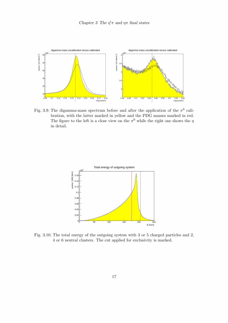
for the π0 and 21 MeV/c2 for the η. Here, the first method of reducing the errorin the energy measurement comes into play, namely the calibration described insection 3.2. As can be seen in figure 3.9, both the π0 and η peaks are improved bythe ECAL calibration. Said improvement is characterised mainly as a shift of thepeak maxima closer to the PDG masses and also as a reduction of their width.

Energy conservation

Conservation of energy requires that

Ebeam + Etarget = EX + Erecoil (3.9)

If an event is exclusive in the sense that each particle created in the primary inter-action is considered in the event selection, this equation will have to hold. As thedifference Erecoil − Etarget is however typically smaller than 340 MeV (see figure 3.13),the exclusivity condition is simplified as a cut on the total energy of charged particlesand neutral calorimeter clusters, with the calorimeter calibration applied. It is requiredto be 175 GeV ≤ EX ≤ 205 GeV. The cut window is chosen to be very wide as thecalorimeter energies introduce a large error into the sum. This will later be mitigatedby a kinematic fit.

15


Fig. 3.7: The position of selected photons on the calorimeters ECAL1 (left) and ECAL2(right), in a logarithmic scale. Both show calorimeters an intensity decreasingoutwards and a rasterisation due to their cell structure. In the left figure, the3 different types of cells present in ECAL1 are clearly visible. Note that onthe right, the cut on the shadow of HCAL1 at the top and bottom was alreadyapplied. In the right figure, several cells appear with different efficiencies thanthe surrounding ones. Quite faintly on the logarithmic scale, the shadow of apipe in the RICH detector appears as a ring with radius ≈ 20 cm.

) [GeV]γγm(0 0.1 0.2 0.3 0.4 0.5 0.6 0.7 0.8 0.9 1

)2ev

ents

/ (0

.5 M

eV/c

0

10

20

30

40

50

60

310×digamma mass

Fig. 3.8: The m(γγ) spectrum, with calibrated energies for events containing two goodclusters. At the lower end of the mass spectrum, the three distinct combinationsof energy thresholds imposed on good clusters from either of the electromagneticcalorimeters are visible. The peak around 135 MeV corresponds to the π0, whilethe decay η → γγ is visible around 548 MeV. The η peak has both a largerwidth and larger background relative to its amplitude.

16


) [GeV]γγm(0.09 0.1 0.11 0.12 0.13 0.14 0.15 0.16 0.17 0.18

)2ev

ents

/ (0

.5 M

eV/c

10

20

30

40

50

60

310×digamma mass uncalibrated versus calibrated

) [GeV]γγm(0.46 0.48 0.5 0.52 0.54 0.56 0.58 0.6 0.62 0.64

)2ev

ents

/ (0

.5 M

eV/c

2

2.5

3

3.5

4

310×digamma mass uncalibrated versus calibrated

Fig. 3.9: The digamma-mass spectrum before and after the application of the π0 cali-bration, with the latter marked in yellow and the PDG masses marked in red.The figure to the left is a close view on the π0 while the right one shows the ηin detail.

E [GeV]0 50 100 150 200 250

even

ts /

(500

MeV

)

0

0.02

0.04

0.06

0.08

0.1

0.12

0.14

0.16

610×Total energy of outgoing system

Fig. 3.10: The total energy of the outgoing system with 3 or 5 charged particles and 2,4 or 6 neutral clusters. The cut applied for exclusivity is marked.

17


) [GeV]γγm(0 0.1 0.2 0.3 0.4 0.5 0.6 0.7 0.8 0.9 1

)2ev

ents

/ (0

.5 M

eV/c

0

10

20

30

40

50

60

310×digamma mass

) [GeV]γγm(0 0.1 0.2 0.3 0.4 0.5 0.6 0.7 0.8 0.9 1

)2ev

ents

/ (0

.5 M

eV/c

0

5

10

15

20

25

30

310×digamma mass, energy conservation

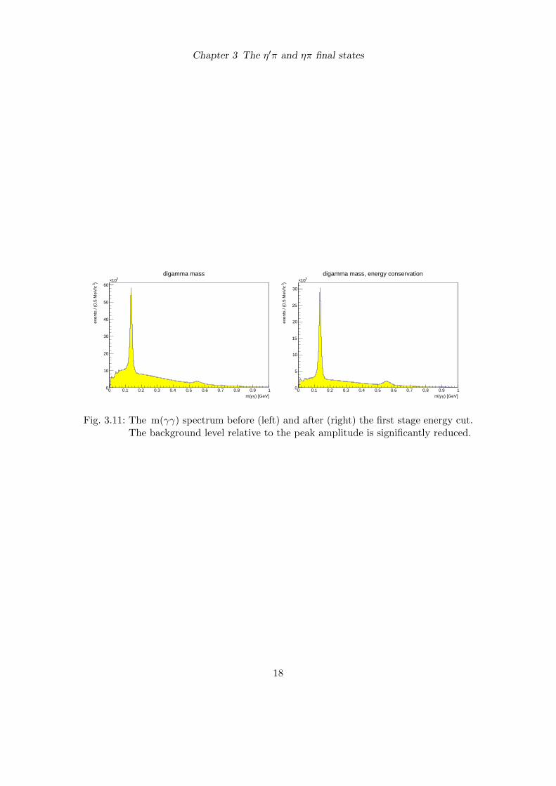
Fig. 3.11: The m(γγ) spectrum before (left) and after (right) the first stage energy cut.The background level relative to the peak amplitude is significantly reduced.

18


Z [cm]-80 -70 -60 -50 -40 -30 -20

even

ts /

(0.5

cm

)

0

0.1

0.2

0.3

0.4

0.5

610×Z position of primary vertex in the second stage preselection

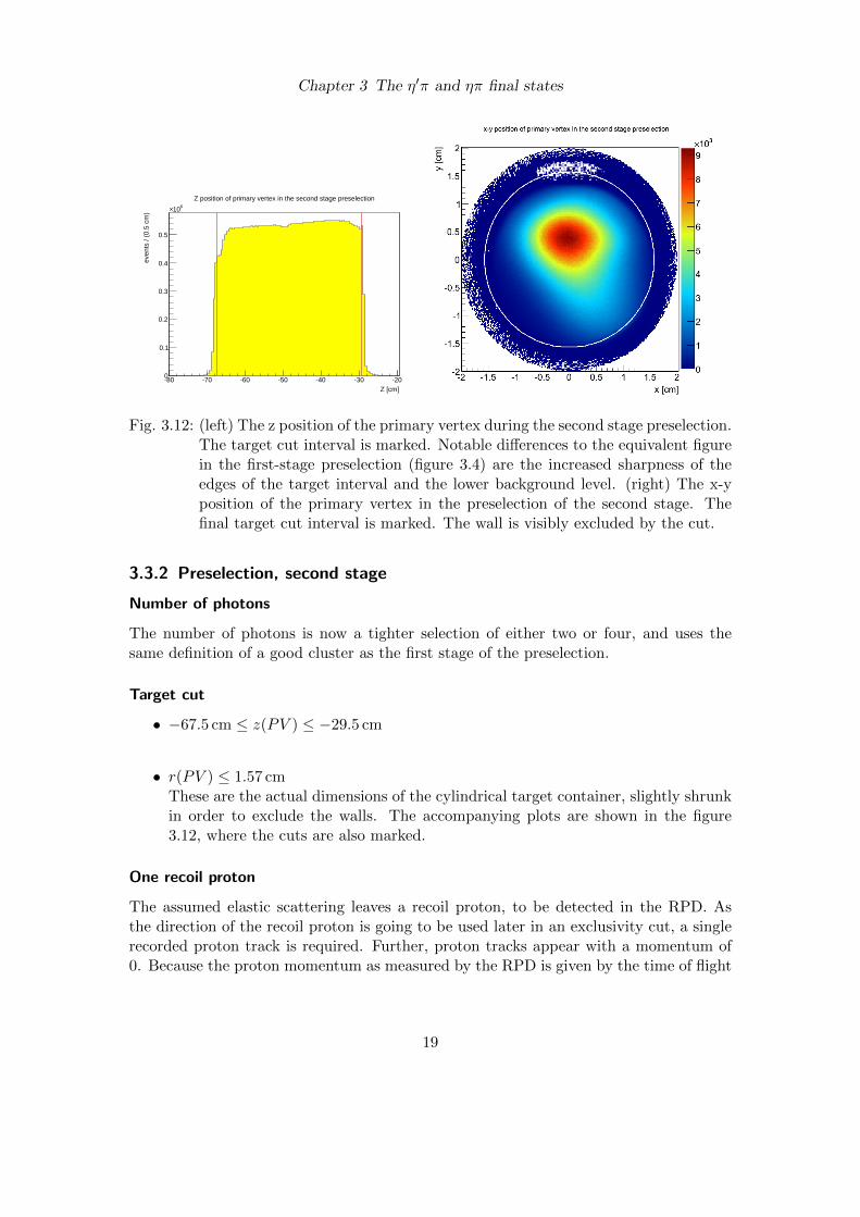
Fig. 3.12: (left) The z position of the primary vertex during the second stage preselection.The target cut interval is marked. Notable differences to the equivalent figurein the first-stage preselection (figure 3.4) are the increased sharpness of theedges of the target interval and the lower background level. (right) The x-yposition of the primary vertex in the preselection of the second stage. Thefinal target cut interval is marked. The wall is visibly excluded by the cut.

3.3.2 Preselection, second stage

Number of photons

The number of photons is now a tighter selection of either two or four, and uses thesame definition of a good cluster as the first stage of the preselection.

Target cut

• −67.5 cm ≤ z(PV ) ≤ −29.5 cm

• r(PV ) ≤ 1.57 cmThese are the actual dimensions of the cylindrical target container, slightly shrunkin order to exclude the walls. The accompanying plots are shown in the figure3.12, where the cuts are also marked.

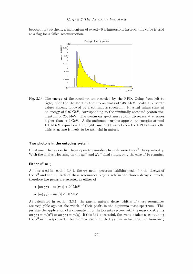
One recoil proton

The assumed elastic scattering leaves a recoil proton, to be detected in the RPD. Asthe direction of the recoil proton is going to be used later in an exclusivity cut, a singlerecorded proton track is required. Further, proton tracks appear with a momentum of0. Because the proton momentum as measured by the RPD is given by the time of flight

19


between its two shells, a momentum of exactly 0 is impossible; instead, this value is usedas a flag for a failed reconstruction.

E [GeV]0.9 1 1.1 1.2 1.3 1.4

even

ts /

(0.6

8 M

eV)

0

0.05

0.1

0.15

0.2

0.25

610×Energy of recoil proton

Fig. 3.13: The energy of the recoil proton recorded by the RPD. Going from left toright, after the the start at the proton mass of 938 MeV, peaks at discretevalues appear, followed by a continuous spectrum. Physical values start atan energy of 0.97 GeV, corresponding to the minimally accepted proton mo-mentum of 250 MeV. The continous spectrum rapidly decreases at energieshigher than ≈ 1 GeV. A discontinuous surplus appears at energies around1.115 GeV, equivalent to a flight time of 4.0 ns between the RPD’s two shells.This structure is likely to be artificial in nature.

Two photons in the outgoing system

Until now, the option had been open to consider channels were two π0 decay into 4 γ.With the analysis focusing on the ηπ− and η′π− final states, only the case of 2γ remains.

Either π0 or η

As discussed in section 3.3.1, the γγ mass spectrum exhibits peaks for the decays ofthe π0 and the η. Each of these resonances plays a role in the chosen decay channels,therefore the peaks are selected as either of

•∣∣m(γγ)−m(π0)

∣∣ < 20 MeV

• |m(γγ)−m(η)| < 50 MeV

As calculated in section 3.3.1, the partial natural decay widths of these resonancesare negligible against the width of their peaks in the digamma mass spectrum. Thisjustifies the application of a kinematic fit of the Lorentz vectors with the mass constraintsm(γγ) = m(π0) or m(γγ) = m(η). If this fit is successful, the event is taken as containingthe π0 or η, respectively. An event where the fitted γγ pair in fact resulted from an η

20


or π0 decay, the error in the photon energy is reduced. This step improves the possibleexclusivity cut, as is detailed in the next section.

Exclusivity

To improve the exclusivity of analysed events, two different types of cuts were used. Theenergy exclusivity cut, detailed in section 3.3.1 is similar to the one performed in thepre-selection. The ∆φ exclusivity cut is motivated as an augmentation of the energyexclusivity cut, which is limited due to the variance in the beam energy. The outgoingsystem for which the exclusivity variables are calculated contains a kinematically fittedphoton pair. The correction to the photon energies made by the kinematic fit leadsto a narrower exclusivity peak and a spreading of the energies of non-exclusive events,and thus a smaller non-ecxclusive background. ∆φ is defined as the angle between theprojections of the momenta ~pX and ~precoil transverse to the beam direction. For anillustration see figure 3.14. It is calculated

∆φ = ^(~pX × ~pbeam, ~pRP × ~pbeam) (3.10)

The interesting property of ∆φ is that it is not kinematically linked to the absolutevalues of the momenta involved, freeing a cut on ∆φ from the beam energy variance.Taking conservation of momentum as the basis of this cut gives

~pX · ~pbeam = (~pbeam − ~pRP) · ~pbeam = −~pRP · ~pbeam (3.11)

Thus, the physically expected value is ∆φ = π, which is the maximum appearing infigure 3.16. The beam direction is measured by the silicon telescope, a series of trackingdetectors upstream from the target. The direction of the recoil proton is measured inthe RPD using the segmentation of its scintillator barrel. Hence, the resolution of themeasurement of ∆φ is dominated by the azimuthal angle resolution of the RPD, whichis π

12 given by the segmentation of the RPD’s shells (see 2.2).

• The energy of the outgoing system with kinematically fitted γγ is limited to therange 186 GeV ≤ EX ≤ 196 GeV.

• From the above calculation, it is demanded that ∆φ ≥ π − π12 ≈ 2.9.

The figure 3.16 shows the correlation between the two exclusivity cuts; that is, a cut oneither of two quantities reduces the non-exclusive background of the other, as well.

3.3.3 Summary

With both stages combined, the preselection reduced the event sample to 7.9 · 10−4 ofits original size. The steps taken to identify single decay channels will again reduce thesample by several orders of magnitude.

21


beam

outg

oing

reco

il

Δφ

RPD, inner shell

Fig. 3.14: Illustration of the quantity ∆φ.

Cut Percentage of events left after the cutStart 100%DT0 trigger 75.07%Best primary vertex 63.65%Target cut 56.16%Number of charged particles ∈ 3, 4, 5 15.85%Charge conservation 9.95%Number of photons ∈ 2, 4, 6 2.26%Energy conservation 0.74%

Table 3.3: Cut statistics for the preselection, first stage.

Cut Percentage of events left after the cutStart of stage 2 100%Number of photons ∈ 2, 4 89.7%Target cut 85.6%One recoil proton 63.0%Two photons 39.4%Two photon kinematic fit 15.1%Exclusivity 10.7%

Table 3.4: Cut statistics for the preselection, second stage.

22


E [GeV]150 160 170 180 190 200 210 220 230 240 250

even

ts /

(200

MeV

)

0

0.02

0.04

0.06

0.08

0.1

0.12

0.14

0.16

0.18

0.2

0.22

610×Total energy of outgoing system including a kinematically fitted photon pair

Fig. 3.15: The energy of the outgoing system with a kinematically fitted γγ pair. Thelimits set for the exclusivity are marked. By comparing with figure 3.10,the kinematic fit can be seen to have the effect of spreading the energies ofbackground events and leaving the exclusivity peak intact.

Fig. 3.16: The energy and ∆φ used in the exclusivity cut are entered into a 2-dimensionalhistogram. The cuts applied on both quantities are marked. The correlationbetween the two cuts is visible.

23


3.4 Final Selection

3.4.1 Second stage, channel ηπ− → (π+π0π−)π−

The state consists of 2 π−, 1 π+ and a π0 which was fitted from 2 γ clusters. Theevent is required to contain a π− so that

∣∣m(π+π−π0)−m(η)∣∣ < 20 MeV/c2, which is

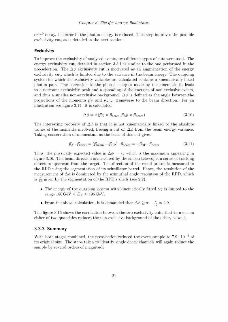
considered an η candidate. This is the case for 7.6% of the events that are considered inthis channel. At this stage, two combinations (using either of the π− respectively) arepossible, of which just one is chosen. In theory, this introduces an ambiguity. However,with m(η) − (2m(π±) + m(π0)) = 164.7 MeV/c2, the decay η → π+π0π− has verylittle phase space. This is visible in the left plot of figure 3.17, where the mass peakcorresponding to the η is located at the lower end of the spectrum and as a result hasvery low “combinatorial“ background. A continuation of the selection (that is, the casewhere an η candidate was found) contains to 1.9% events in which an ambiguity betweentwo η candidates occurs.Using the chosen π−, the (π+π−π0) is fitted to the η mass. One might suspect that twoindependent fits acting on the same variables with different constraints might interferewith each other, that the compliance with the first fit hypothesis will be inadvertantlyworsened by the second one. As can be seen in figure 3.18 by comparing the digamma-mass directly before and after this fit, the originally present π0 peak only improves inquality, that is becomes narrower. This speaks in favour of the application of the fit andthe selection of events.The resulting final selection is ηπ−, of which the mass spectrum is shown in the righthalf of figure 3.17. The spectrum is dominated by the a2(1320.

]2) [GeV/c0π-π+πm(

0.4 0.5 0.6 0.7 0.8 0.9 1

)2ev

ents

/(1

MeV

/c

0

2

4

6

8

10

310×, two combinationsγγ fitted from 0π systems with an 0π-π+πmass

]2) [GeV/c-πηm(

1 1.5 2 2.5 3 3.5 4 4.5

)2ev

ents

/(4

MeV

/c

0

0.2

0.4

0.6

0.8

1

1.2

1.4

1.6

1.8

310×

0π-π+π fitted from η systems with an η-π+πmass

Fig. 3.17: Two relevant kinematic plots for the decay channel of ηπ− → (π+π0π−)π−.(left) The π+π−π0) mass spectrum, filled for each of the two available combi-nations. The η mass window is marked. (right) The (ηπ−) mass spectrum forthe final selection.

24


]2) [GeV/cγγm(

0.1 0.11 0.12 0.13 0.14 0.15 0.16 0.17

)2ev

ents

/(0.

5 M

eV/c

0

1

2

3

4

5

6

310×η to γγ-π+πdigamma mass after kinematic fit

Fig. 3.18: The digamma mass spectrum is compared before and after a kinematic fit ofa (π+π−γγ) within an η mass window to the η mass, where the γγ was alsopreviously selected as a π0 candidate.

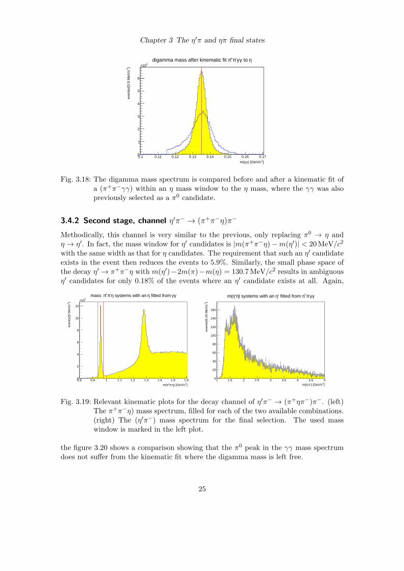
3.4.2 Second stage, channel η′π− → (π+π−η)π−

Methodically, this channel is very similar to the previous, only replacing π0 → η andη → η′. In fact, the mass window for η′ candidates is |m(π+π−η)−m(η′)| < 20 MeV/c2

with the same width as that for η candidates. The requirement that such an η′ candidateexists in the event then reduces the events to 5.9%. Similarly, the small phase space ofthe decay η′ → π+π−η with m(η′)−2m(π)−m(η) = 130.7 MeV/c2 results in ambiguousη′ candidates for only 0.18% of the events where an η′ candidate exists at all. Again,

]2) [GeV/cη-π+πm(

0.8 0.9 1 1.1 1.2 1.3 1.4 1.5 1.6

)2ev

ents

/(5

MeV

/c

0

2

4

6

8

10

12


]2) [GeV/c-π'ηm(

1 1.5 2 2.5 3 3.5 4 4.5 5

)2ev

ents

/(6.

25 M

eV/c

0

20

40

60

80

100

120

140

160

γγ-π+π' fitted from η) systems with an π'ηm(

Fig. 3.19: Relevant kinematic plots for the decay channel of η′π− → (π+ηπ−)π−. (left)The π+π−η) mass spectrum, filled for each of the two available combinations.(right) The (η′π−) mass spectrum for the final selection. The used masswindow is marked in the left plot.

the figure 3.20 shows a comparison showing that the π0 peak in the γγ mass spectrumdoes not suffer from the kinematic fit where the digamma mass is left free.

25


The main difference lies in the mass spectrum of the η′π− final state, which is shown onthe right side of figure 3.19. Instead of dominating the spectrum, the a2(1320) appearson the rising edge around 1.3 GeV/c2.

]2) [GeV/cγγm(

0.48 0.5 0.52 0.54 0.56 0.58 0.6 0.62

)2ev

ents

/(0.

5 M

eV/c

0

0.5

1

1.5

2

2.5

310×'η to γγ-π+πdigamma mass after kinematic fit

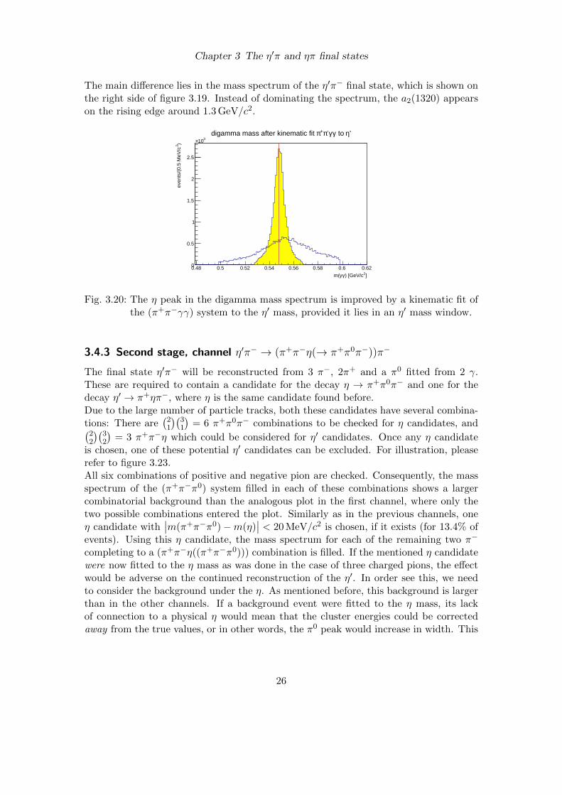
Fig. 3.20: The η peak in the digamma mass spectrum is improved by a kinematic fit ofthe (π+π−γγ) system to the η′ mass, provided it lies in an η′ mass window.

3.4.3 Second stage, channel η′π− → (π+π−η(→ π+π0π−))π−

The final state η′π− will be reconstructed from 3 π−, 2π+ and a π0 fitted from 2 γ.These are required to contain a candidate for the decay η → π+π0π− and one for thedecay η′ → π+ηπ−, where η is the same candidate found before.Due to the large number of particle tracks, both these candidates have several combina-tions: There are

(21

)(31

)= 6 π+π0π− combinations to be checked for η candidates, and(

22

)(32

)= 3 π+π−η which could be considered for η′ candidates. Once any η candidate

is chosen, one of these potential η′ candidates can be excluded. For illustration, pleaserefer to figure 3.23.All six combinations of positive and negative pion are checked. Consequently, the massspectrum of the (π+π−π0) system filled in each of these combinations shows a largercombinatorial background than the analogous plot in the first channel, where only thetwo possible combinations entered the plot. Similarly as in the previous channels, oneη candidate with

∣∣m(π+π−π0)−m(η)∣∣ < 20 MeV/c2 is chosen, if it exists (for 13.4% of

events). Using this η candidate, the mass spectrum for each of the remaining two π−

completing to a (π+π−η((π+π−π0))) combination is filled. If the mentioned η candidatewere now fitted to the η mass as was done in the case of three charged pions, the effectwould be adverse on the continued reconstruction of the η′. In order see this, we needto consider the background under the η. As mentioned before, this background is largerthan in the other channels. If a background event were fitted to the η mass, its lackof connection to a physical η would mean that the cluster energies could be correctedaway from the true values, or in other words, the π0 peak would increase in width. This

26


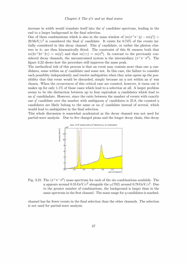
increase in width would translate itself into the η′ candidate spectrum, leading in theend to a larger background in the final selection.One of these combinations which is also in the mass window of |m(π+π−η)−m(η′)| <20 MeV/c2 is considered the final η′ candidate. It exists for 0.74% of the events ini-tially considered in this decay channel. This η′ candidate, or rather the photon clus-ters in it, are then kinematically fitted. The constraint of this fit ensures both thatm(2π+2π−2γ) = m(η′) and that m(γγ) = m(π0). In contrast to the previously con-sidered decay channels, the unconstrained system is the intermediary (π+π−π0). Thefigure 3.22 shows how the procedure still improves the mass peak.The methodical risk of this process is that an event may contain more than one η can-didates, some within an η′ candidate and some not. In this case, the failure to considereach possiblity independently and resolve ambiguities when they arise opens up the pos-sibility that this event would be discarded, simply because an η not within an η′ waschosen. When the occurrences of this critical case are counted, however, it turns out itmakes up for only 1.1% of those cases which lead to a selection at all. A larger problemseems to be the distinction between up to four equivalent η candidates which lead toan η′ candidadate. However, since the ratio between the number of events with exactlyone η′ candidate over the number with ambiguous η′ candidates is 25.8, the counted ηcandidates are likely belong to the same or no η′ candidate instead of several, whichwould lead to ambiguities in the final selection.This whole discussion is somewhat academical as the decay channel was not used forpartial-wave analysis. Due to five charged pions and the longer decay chain, this decay


0.4 0.5 0.6 0.7 0.8 0.9 1

)2ev

ents

/(1

MeV

/c

0

2

4

6

8

10

12

310×, six combinationsγγ fitted from 0π systems with an 0π-π+πmass

Fig. 3.21: The (π+π−π0) mass spectrum for each of the six combinations available. Theη appears around 0.55 GeV/c2 alongside the ω(782) around 0.78 GeV/c2. Dueto the greater number of combinations, the background is larger than in thesame spectrum in the first channel. The mass range for η candidates is marked.

channel has far fewer events in the final selection than the other channels. The selectionis not used for partial-wave analysis.

27



0.48 0.5 0.52 0.54 0.56 0.58 0.6 0.62

)2ev

ents

/(2

MeV

/c

0

100

200

300

400

500

600

700

800

900

'η) to γγ-π+π-π+π' candidate and after the fit from (η) contained in an 0π-π+πm(

Fig. 3.22: Shown is the η peak in a selection of η candidates which are part of an η′

candidate. In the yellow histogram, a kinematic fit is applied that uses twoconstraints; one on the mass of the γγ which appears in the η candidate to theπ0 mass; and one constraining the η′ candidate formed with this η candidateand two additional charged pions to the η′ mass. We observe that the peakbecomes slightly narrower and spreads itself out along the eges. This figureplays a similar role as figure 3.20 and figure 3.18; only it shows that a thirdconstraint would not be a good idea.

π+1

π+2

π−1 π

−2 π

−3 π−

1 π−2 π

−3 π−

1 π−2 π

−3

π η3η6

η2η5

η1η4

η1η2

1

η4η5

η1

η3

η4

η6

η2η3

η5η6

η'1

η'2

η'3

Fig. 3.23: The combinatorics in the five-track channel. Each box is one of three potentialη′ candidates, containing four of six potential η candidates constructed withcombinations of one of three π− and one of two π+.

28


]2) [GeV/cη-π+πm(

0.8 0.9 1 1.1 1.2 1.3 1.4 1.5 1.6

)2ev

ents

/(5

MeV

/c

0

0.5

1

1.5

2

2.5310×

γγ fitted from 0π) and 0π-π+π candidate (η) with an η-π+πm(

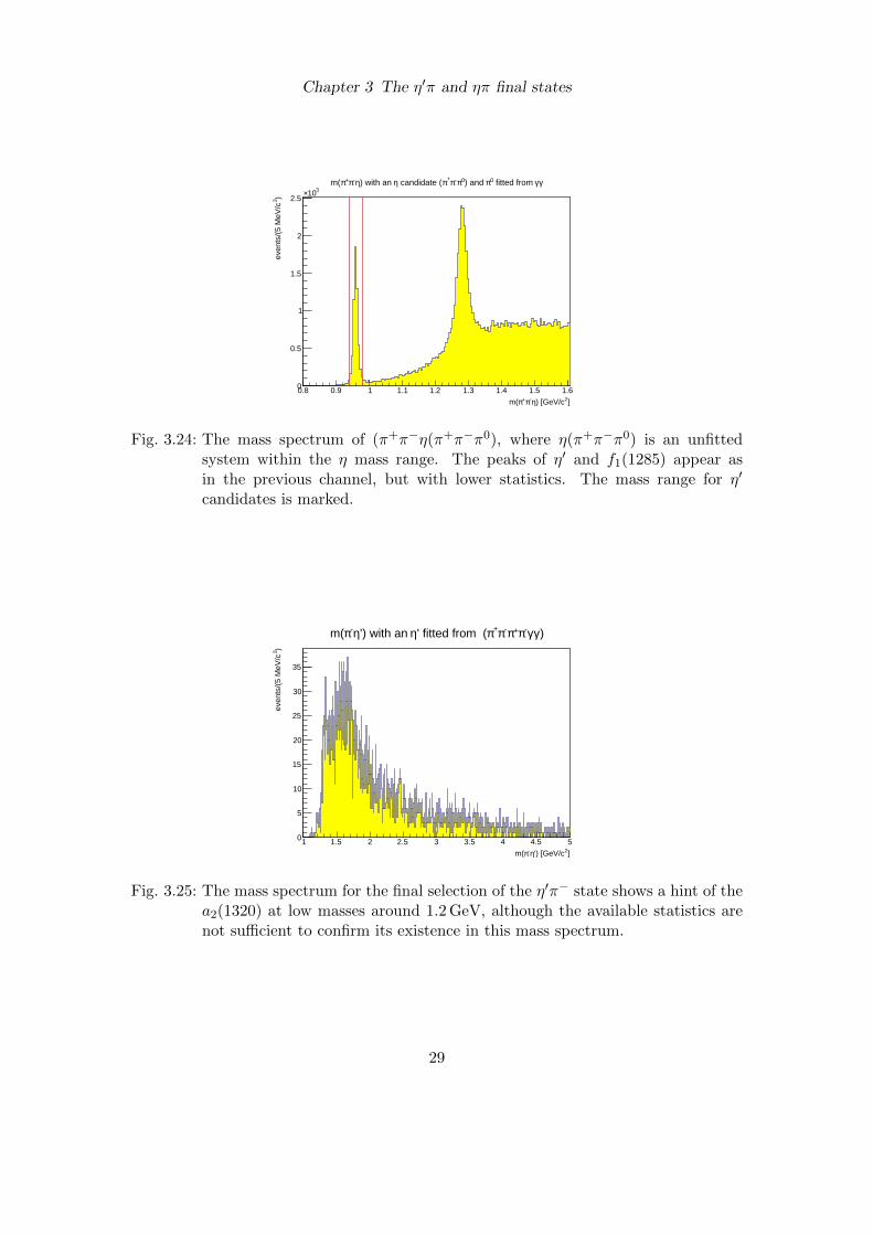
Fig. 3.24: The mass spectrum of (π+π−η(π+π−π0), where η(π+π−π0) is an unfittedsystem within the η mass range. The peaks of η′ and f1(1285) appear asin the previous channel, but with lower statistics. The mass range for η′

candidates is marked.

]2') [GeV/cη-πm(

1 1.5 2 2.5 3 3.5 4 4.5 5

)2ev

ents

/(5

MeV

/c

0

5

10

15

20

25

30

35

)γγ-π+π-π+π' fitted from (η') with an η-πm(

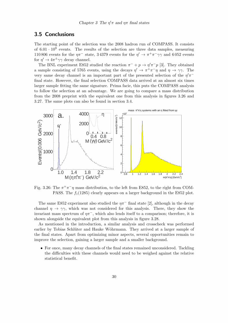
Fig. 3.25: The mass spectrum for the final selection of the η′π− state shows a hint of thea2(1320) at low masses around 1.2 GeV, although the available statistics arenot sufficient to confirm its existence in this mass spectrum.

29


3.5 Conclusions

The starting point of the selection was the 2008 hadron run of COMPASS. It consistsof 6.01 · 109 events. The results of the selection are three data samples, measuring110 806 events for the ηπ− state, 3 4379 events for the η′ → π+π−γγ and 6 052 eventsfor η′ → 4π±γγ decay channel.

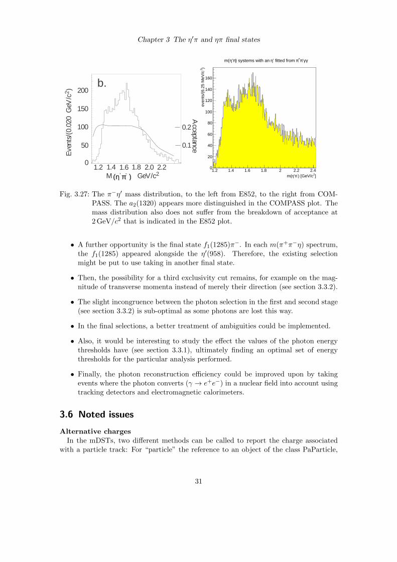
The BNL experiment E852 studied the reaction π− + p → η′π−p [3]. They obtaineda sample consisting of 5765 events, using the decays η′ → π+π−η and η → γγ. Thevery same decay channel is an important part of the presented selection of the η′π−

final state. However, the final selection COMPASS data arrived at an almost six timeslarger sample fitting the same signature. Prima facie, this puts the COMPASS analysisto follow the selection at an advantage. We are going to compare a mass distributionfrom the 2008 preprint with the equivalent one from this analysis in figures 3.26 and3.27. The same plots can also be found in section 3.4.

M GeV/c2(γγ)0.4 0.8

2000

4000

0

η

(ηπ π )+ -M GeV/c21.0 1.4 1.8 2.2

η'

Eve

nts/

(0.0

06 G

eV/c

)2

1000

3000

0

2000

a..

]2) [GeV/cη-π+πm(0.8 1 1.2 1.4 1.6 1.8 2 2.2 2.4

)2ev

ents

/(5

MeV

/c

0

2

4

6

8

10

12


Fig. 3.26: The π+π−η mass distribution, to the left from E852, to the right from COM-PASS. The f1(1285) clearly appears on a larger background in the E852 plot.

The same E852 experiment also studied the ηπ− final state [2], although in the decaychannel η → γγ, which was not considered for this analysis. There, they show theinvariant mass spectrum of ηπ−, which also lends itself to a comparison; therefore, it isshown alongside the equivalent plot from this analysis in figure 3.28.

As mentioned in the introduction, a similar analysis and crosscheck was performedearlier by Tobias Schluter and Hauke Wohrmann. They arrived at a larger sample ofthe final states. Apart from optimizing minor aspects, several opportunities remain toimprove the selection, gaining a larger sample and a smaller background.

• For once, many decay channels of the final states remained unconsidered. Tacklingthe difficulties with these channels would need to be weighed against the relativestatistical benefit.

30


M GeV/c(η π )(η π )- 2'1.2 1.4 1.6 1.8

Eve

nts/

(0.0

20 G

eV/c

)2

50

150

0

100

2.0 2.2

200b.

0.1

0.2

Acceptance

]2) [GeV/c-π'ηm(

1.2 1.4 1.6 1.8 2 2.2 2.4

)2ev

ents

/(6.

25 M

eV/c

0

20

40

60

80

100

120

140

160

γγ-π+π' fitted from η) systems with an π'ηm(

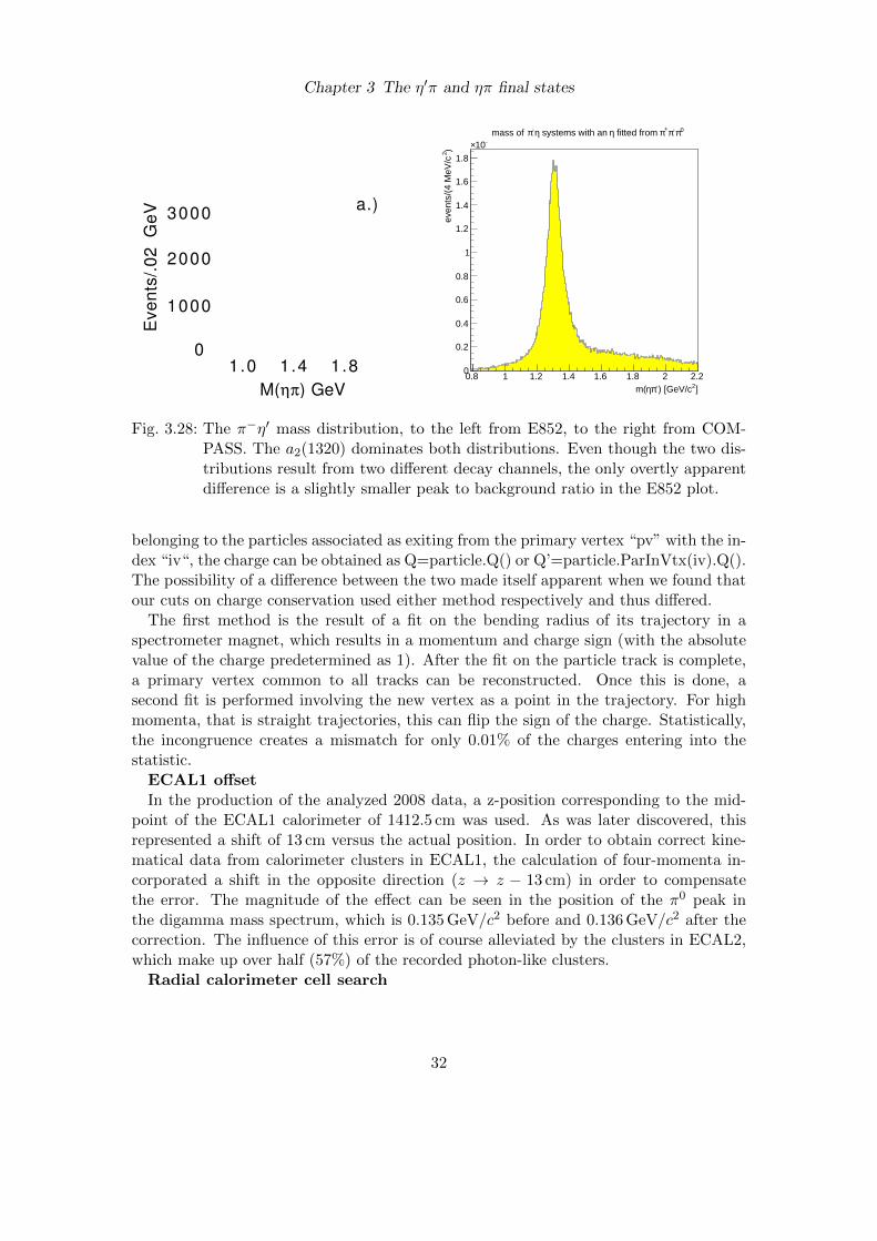
Fig. 3.27: The π−η′ mass distribution, to the left from E852, to the right from COM-PASS. The a2(1320) appears more distinguished in the COMPASS plot. Themass distribution also does not suffer from the breakdown of acceptance at2 GeV/c2 that is indicated in the E852 plot.

• A further opportunity is the final state f1(1285)π−. In each m(π+π−η) spectrum,the f1(1285) appeared alongside the η′(958). Therefore, the existing selectionmight be put to use taking in another final state.

• Then, the possibility for a third exclusivity cut remains, for example on the mag-nitude of transverse momenta instead of merely their direction (see section 3.3.2).

• The slight incongruence between the photon selection in the first and second stage(see section 3.3.2) is sub-optimal as some photons are lost this way.

• In the final selections, a better treatment of ambiguities could be implemented.

• Also, it would be interesting to study the effect the values of the photon energythresholds have (see section 3.3.1), ultimately finding an optimal set of energythresholds for the particular analysis performed.

• Finally, the photon reconstruction efficiency could be improved upon by takingevents where the photon converts (γ → e+e−) in a nuclear field into account usingtracking detectors and electromagnetic calorimeters.

3.6 Noted issues

Alternative chargesIn the mDSTs, two different methods can be called to report the charge associated

with a particle track: For “particle” the reference to an object of the class PaParticle,

31


M(ηπ) GeV

1.0 1.4 1.8

3000

2000

1000

0

Eve

nts

/.0

2 G

eV a.)

]2) [GeV/c-πηm(0.8 1 1.2 1.4 1.6 1.8 2 2.2

)2ev

ents

/(4

MeV

/c

0

0.2

0.4

0.6

0.8

1

1.2

1.4

1.6

1.8

310×

0π-π+π fitted from η systems with an η-πmass of

Fig. 3.28: The π−η′ mass distribution, to the left from E852, to the right from COM-PASS. The a2(1320) dominates both distributions. Even though the two dis-tributions result from two different decay channels, the only overtly apparentdifference is a slightly smaller peak to background ratio in the E852 plot.

belonging to the particles associated as exiting from the primary vertex “pv” with the in-dex “iv“, the charge can be obtained as Q=particle.Q() or Q’=particle.ParInVtx(iv).Q().The possibility of a difference between the two made itself apparent when we found thatour cuts on charge conservation used either method respectively and thus differed.

The first method is the result of a fit on the bending radius of its trajectory in aspectrometer magnet, which results in a momentum and charge sign (with the absolutevalue of the charge predetermined as 1). After the fit on the particle track is complete,a primary vertex common to all tracks can be reconstructed. Once this is done, asecond fit is performed involving the new vertex as a point in the trajectory. For highmomenta, that is straight trajectories, this can flip the sign of the charge. Statistically,the incongruence creates a mismatch for only 0.01% of the charges entering into thestatistic.

ECAL1 offsetIn the production of the analyzed 2008 data, a z-position corresponding to the mid-

point of the ECAL1 calorimeter of 1412.5 cm was used. As was later discovered, thisrepresented a shift of 13 cm versus the actual position. In order to obtain correct kine-matical data from calorimeter clusters in ECAL1, the calculation of four-momenta in-corporated a shift in the opposite direction (z → z − 13 cm) in order to compensatethe error. The magnitude of the effect can be seen in the position of the π0 peak inthe digamma mass spectrum, which is 0.135 GeV/c2 before and 0.136 GeV/c2 after thecorrection. The influence of this error is of course alleviated by the clusters in ECAL2,which make up over half (57%) of the recorded photon-like clusters.

Radial calorimeter cell search

32


A bug in the PaCaloClus::iCell() method responsible for finding a cell number corre-sponding to (x, y) coordinates led to segementation errors when applying the calibrationto clusters from different calorimeters. The method uses a lookup table of radii forvarious cells in order minimize the number of checked cells when the cell index for acertain x− y position needs to be found by exploiting the fact that the density of clus-ters decreases outwards. Tobias Schluter discovered the error to stem from an incorrectinitialisation of the mentioned lookup table, which resulted in a table specific to onecalorimeter being used for the other.

33

Chapter 4

Acknowledgements

I would like to thank Professor Stephan Paul of the chair E18 for supplying me with thesubject of this thesis and agreeing to give the work the nature of a cross-check. This hadthe effect of bringing me into close contact with actually ongoing analysis and a wealth ofknowledge and experience in the form of Tobias Schluter. Thanks go to him for puttingup with my questions and misguided efforts, supporting me in making all the relevantdeadlines, and discovering an uncounted number of bugs, both in my code, in a Phastlibrary, and those in his own which I failed to notice, using his superior programmingskills. Further than that, without his methods of cluster calibration and constrainedfitting, this thesis would have significantly less to talk about, and without his gHistlibrary I would have been hestitant to add many plots which later might have turnedout to be meaningful. No little amount of praise is due to Florian Haas for getting mestarted very quickly from the point of having no experience in C++, ROOT or Phastto using all three and guiding me through the final phase of concentrating all thoseweeks spent hacking away at user event functions into a thesis of 34 pages. Boris Grubealso gave far too much of his time, being readily available for many technical problemsand stylistic guidance. Stefan Pfluger showed me the use of several helper libraries andSebastian Uhl provided the LaTeX template on which the style of this thesis is based.

34

Bibliography

[1] J. N. Hedditch et al. “1+ exotic meson at light quark masses”. Phys. Rev. D72(2005) 114507.

[2] E852 Collaboration, D. Thompson et al., Evidence for Exotic Meson Productionin the Reaction π−p → ηπ−p at 18 GeV/c, Phys. Rev. Lett. 79 (1997) 16301633,arXiv:hep-ex/9705011.

[3] E852 Collaboration, E. I. Ivanov et al., Observation of exotic meson productionin the reaction π−p → η′π−p at 18 GeV/c, Phys. Rev. Lett. 86 (2001) 39773980,arXiv:hep-ex/0101058.

[4] Tobias Schluter, “A code for kinematic fitting with constraints from intermediateparticle masses”, COMPASS note 2007-10

[5] Tobias Schluter, “Overview of neutral hadron channel analysis”, COMPASS Col-laboration meeting, March 2010

[6] L. Gatignon, M. Leberig et al., “The M2 Beam Line”

[7] COMPASS Collaboration, P. Abbon et al., “The COMPASS Experiment at CERN”,Nucl. Instr. and Meth. A 577 (2007) 455518, arXiv:hep-ex/0703049

[8] Tobias Schluter et al., “Partial-wave analysis of 2008 η′π− data” - release discussionat the COMPASS Analysis Meeting on June 2nd, 2011.

35

Analysis of the 0 Final States in COMPASS Data 1 Introduction This Bachelor’s thesis describes for...

Documents

Transcript of Analysis of the 0 Final States in COMPASS Data 1 Introduction This Bachelor’s thesis describes for...